Post-merger gravitational-wave signal from neutron-star binaries: a new look at an old problem

Abstract

The spectral properties of the post-merger gravitational-wave signal from a binary of neutron stars encodes a variety of information about the features of the system and of the equation of state describing matter around and above nuclear saturation density. Characterising the properties of such a signal is an “old” problem, which first emerged when a number of frequencies were shown to be related to the properties of the binary through “quasi-universal” relations. Here we take a new look at this old problem by computing the properties of the signal in terms of the Weyl scalar $\psi_{4}$. In this way, and using a database of more than 100 simulations, we provide the first evidence for a new instantaneous frequency, $f^{\psi_{4}}_{0}$, associated with the instant of quasi time-symmetry in the postmerger dynamics, and which also follows a quasi-universal relation. We also derive a new quasi-universal relation for the merger frequency $f^{h}_{\rm mer}$, which provides a description of the data that is four times more accurate than previous expressions while requiring fewer fitting coefficients. Finally, consistently with the findings of numerous studies before ours, and using an enlarged ensamble of binary systems we point out that the $\ell=2,m=1$ gravitational-wave mode could become comparable with the traditional $\ell=2,m=2$ mode on sufficiently long timescales, with strain amplitudes in a ratio $|h^{21}|/|h^{22}|\sim 0.1-1$ under generic orientations of the binary, which could be measured by present detectors for signals with large signal-to-noise ratio or by third-generation detectors for generic signals should no collapse occur.

1 Introduction

The observation of a gravitational-wave (GW) signal from the binary neutron-star (BNS) merger event GW170817 (The LIGO Scientific Collaboration & The Virgo Collaboration, 2017), and the detection of an electromagnetic (EM) counterpart, has testified the enormous potential of GW astronomy. Starting from early works with simplified equations of state (EOSs) (see, e.g.,  Shibata et al., 2005; Anderson et al., 2008; Liu et al., 2008; Baiotti et al., 2008; Hotokezaka et al., 2011), increasingly more comprehensive simulations of these events, which involve an ever more detailed description of the microphysics (Bauswein et al., 2019; De Pietri et al., 2019; Gieg et al., 2019; Tootle et al., 2022; Most et al., 2022; Camilletti et al., 2022; Ujevic et al., 2023), of the magnetic-field evolution (Rezzolla et al., 2011; Dionysopoulou et al., 2013; Ciolfi et al., 2019; Sun et al., 2022; Zappa et al., 2023), and its amplification (Kiuchi et al., 2015; Palenzuela et al., 2022; Chabanov et al., 2023), and of transport of neutrinos (Foucart et al., 2022; Zappa et al., 2023), allow one to make predictions from the early inspiral up to the long-term evolution of the postmerger remnant (De Pietri et al., 2020; Kiuchi et al., 2022). During each stage in the evolution of the binary, the features of the GW and EM signals change in a characteristic manner, encoding information on the properties of the constituent neutron stars and of the hypermassive neutron star (HMNS) produced after the merger and, hence, on the governing EOS.

Characterising the properties of the post-merger GW signal is a rather “old” problem, which has first emerged when a number of peculiar frequencies were shown to be related with the properties of the binary through quasi-universal relations, i.e., relations that are almost independent of the specific EOS. These relations have been suggested for the GW frequency at merger $f_{\rm mer}$ (Read et al., 2013; Bernuzzi et al., 2014; Takami et al., 2015; Rezzolla & Takami, 2016; Most et al., 2019; Bauswein et al., 2019; Weih et al., 2020; Gonzalez et al., 2022), the dominant frequency in the postmerger spectrum $f_{2}$ (see, e.g.,  Oechslin & Janka, 2007; Bauswein & Janka, 2012; Read et al., 2013; Rezzolla & Takami, 2016; Gonzalez et al., 2022), and other frequencies identifiable in the transient period right after the merger (Bauswein & Stergioulas, 2015; Takami et al., 2015; Rezzolla & Takami, 2016). Fits to these quasi-universal relations have been employed in a number of studies (see, e.g.,  (Bauswein et al., 2016; Baiotti & Rezzolla, 2017) for some reviews). These EOS-insensitive relations can help enormously in constraining the EOS of matter at nuclear densities, marking the possible appearance of phase transitions (Most et al., 2019; Weih et al., 2020; Liebling et al., 2021; Prakash et al., 2021; Fujimoto et al., 2023; Tootle et al., 2022; Espino et al., 2023), inform waveform models (Bose et al., 2018; Breschi et al., 2019); however, see Raithel & Most (2022) for possible violations of these relations.

Another relatively “old” problem in the characterisation of the GW signal from BNS is the one about the relative weight of the lower-order multipole $\ell=2,m=1$. Numerical simulations have highlighted that the HMNS can be subject to a nonaxisymmetric instability that powers the growth of $\ell=2,m=1$ mode of the rest-mass density distribution and, hence, of the corresponding GW signal (see, e.g.,  East et al., 2015; Lehner et al., 2016a, b; Radice et al., 2016; East et al., 2019; Papenfort et al., 2022). This mode can already be seeded by the initial asymmetry of the system in the unequal-mass case, or develop by the shearing of the contact layers of the binary constituents upon merger. While the $\ell=2,m=2$ GW mode is the primary contributor to the GW signal, it is damped faster than the other modes leading to interesting secular behaviours.

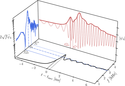
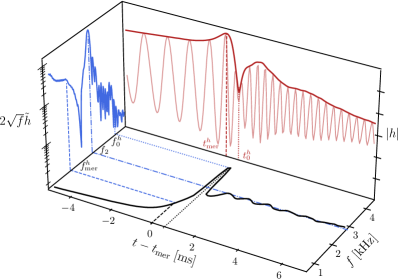
Figure 1: 3D representation of the complete information in the GW signal from a representative binary (Tootle et al., 2022). The left panel shows the $\ell=2,m=2$ mode of the GW signal $\psi_{4}(t)$ (light red) and its amplitude $|\psi_{4}(t)|$ (dark red), the instantaneous frequency $f_{{}_{\rm GW}}(t)$ (black), and the power spectral density (PSD) $\sqrt{2}f\,\tilde{\psi}_{4}$ (blue) as a function of the frequency $f$. Also indicated are the frequency at merger $f_{\rm mer}^{\psi_{4}}$, the frequency at quasi time-symmetry $f^{\psi_{4}}_{0}$, the dominant frequency of the HMNS emission $f_{2}$, and the corresponding times where these frequencies appear. The right panel shows the same quantities but when computed in terms of the GW strain.

We here take a new look at both of these old problems by considering the spectral properties of the GW signal when computed in terms of the Weyl scalar $\psi_{4}$. In this way, we are able to find three novel features that can enrich our understanding of the GW signal from BNS mergers. In particular, we first highlight the presence of a new instantaneous frequency, which we dub $f^{\psi_{4}}_{0}$, that can be associated with the instant of quasi time-symmetry in the postmerger dynamics. Interestingly, we find that a quasi-universal relation exists for $f^{\psi_{4}}_{0}$ as a function of the tidal deformability $\kappa_{2}^{{}_{T}}$ and of the binary mass ratio $q$. Second, by employing a large number of BNS simulations, some of which are taken from the CoRe database (Gonzalez et al., 2022), we obtain a new quasi-universal relation for $f_{\rm mer}$ as a function of $\kappa_{2}^{{}_{T}}$ and $q$ that not only requires a smaller number of coefficients, but also provides a more accurate description of the data. Finally, as already suggested in (Papenfort et al., 2022), we provide evidence that the $\ell=2,m=1$ GW mode could become the most powerful mode on secular timescales after the merger.

2 Numerical and physical framework

Our analysis is based on the GW signal computed via numerical simulations of BNS mergers in full general relativity computed with the codes described in (Radice et al., 2014a, b; Most et al., 2019a, b; Papenfort et al., 2021; Tootle et al., 2021) and using a number of different EOSs (see below). In addition, we employ part of the data contained in the CoRe database (Gonzalez et al., 2022), from where we select only simulations with the highest-resolution. The combined data of $118$ irrotational binaries covers the range $q:=M_{2}/M_{1}\in[0.485,1]$ in the mass ratio, $M:=M_{1}+M_{2}\in[2.4,3.33]~{}M_{\odot}$ in the total ADM mass at infinite separation, and $\kappa_{2}^{{}_{T}}\in[33,458]$ in the tidal deformability. The dataset comprises a variety of EOSs including some with quark matter (Prakash et al., 2021; Logoteta, Domenico et al., 2021; Alford et al., 2005; Demircik et al., 2022; Tootle et al., 2022).

A crucial role in our analysis is played by the use of the Weyl scalar $\psi_{4}$ in place of the standard dimensionless strain polarisations $h_{+,\times}$. The two quantities are mathematically equivalent and related by two time derivatives (i.e., $\psi_{4}=\partial^{2}_{t}(h_{+}-ih_{\times})$; see (Bishop & Rezzolla, 2016) for a review). However, while $\psi_{4}$ is computed from the simulations, $h_{+,\times}$ are obtained after a nontrivial double time integration (the transformation from $h_{+,\times}$ to is $\psi_{4}$ trivial as it involves derivatives and not integrals; see (Calderon Bustillo et al., 2022) for a data-analysis framework based on $\psi_{4}$, which can obviously be employed for all types of compact-object binaries). More importantly, the evolution of the GW frequency from $\psi_{4}$ is less rapid than from the strain, i.e., $\partial_{t}\ln f^{\psi_{4}}_{{}_{\rm GW}}(t)\ll\partial_{t}\ln f^{h}_{{}_{\rm GW}}(t)$, thus making it easier and more robust to characterise the features of the $\psi_{4}$ GW signal. In this sense, while $\psi_{4}$ and $h_{+,\times}$ are related by simple time derivatives, the analysis carried out with the former does provide additional information as it allows for the determination of properties that are harder to capture with the latter.

3 Old and new frequencies

Figure 1 reports the complete information of the GW signal from a representative binary in our sample. Using a 3D representation, we report on the left the $\ell=2,m=2$ mode of the GW signal $\psi_{4}(t)$ (light red) and its amplitude $|\psi_{4}(t)|$ (dark red), the instantaneous frequency $f^{\psi_{4}}_{{}_{\rm GW}}(t)$ (black), and the power spectral density (PSD) $\sqrt{2}f\,\tilde{\psi}_{4}$ (blue) as a function of the frequency $f$ (see Rezzolla & Takami, 2016, for details on the definition). Also indicated are the three main frequencies in our analysis: the frequency at merger $f_{\rm mer}^{\psi_{4}}$, i.e., the GW frequency at the first maximum of $|\psi_{4}|$, the frequency at quasi time-symmetry $f^{\psi_{4}}_{0}$, i.e., the GW frequency at the first minimum of $|\psi_{4}|$, and the dominant frequency of the HMNS emission $f_{2}^{\psi_{4}}$. To help the eye, we also mark with lines the corresponding times $t^{\psi_{4}}_{\rm mer}$ (dashed), $t^{\psi_{4}}_{0}$ (dotted), and frequencies (dashed, dotted and dot-dashed respectively). The right panel of Fig. 1 shows the same quantities but when computed from the strain. By comparing the black lines in the left and right panels it is straightforward to realise that the variation of $f^{h}_{{}_{\rm GW}}(t)$ is much larger than that in $f^{\psi_{4}}_{{}_{\rm GW}}(t)$ over the same interval of $\sim 1\,$ms after the merger. It is this very rapid change in $f^{h}_{{}_{\rm GW}}(t)$ that makes the identification of $f^{h}_{0}$ extremely difficult, if not impossible. Note also that while in both representations $f_{\rm mer}<f_{2}<f_{0}$, the numerical values of the various quantities are similar but not identical. However, $f_{2}^{\psi_{4}}\simeq f_{2}^{h}$ to very good precision (the largest differences are $\lesssim 4\%$) simply because this frequency is relative to a mostly monochromatic GW signal; hence, hereafter we simply assume $f_{2}^{\psi_{4}}=f_{2}^{h}=:f_{2}$. Finally, because in all representations $f_{0}$ is largest frequency measured, even a crude measure of largest frequency in the signal will serve as a first estimate of the $f_{0}$ frequency.

Besides marking the time of the first amplitude minimum, from a physical point of view $t^{\psi_{4}}_{0}$ corresponds to the time when the two stellar cores have reached the minimum separation and are about to bounce-off each other. At this instant, the corresponding amplitude of $\psi_{4}$ shows a clear minimum, while the instantaneous GW frequency a local maximum [the discussion in the Supplemental Material (SM) illustrates this behaviour very clearly by employing the toy model introduced in (Takami et al., 2015)].

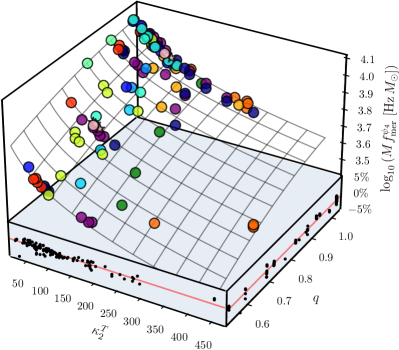
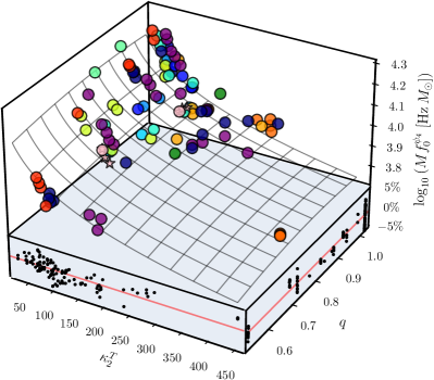
Figure 2: 3D representation of the GW frequencies $f^{\psi_{4}}_{\rm mer}$ and $f^{\psi_{4}}_{0}$ as measured from the data (coloured circles) and presented as a function of $\kappa^{{}_{T}}_{2}$ and $q$. Also reported are the best-fit surfaces, while shown below are the relative errors of the fit in the two principal directions. Stars mark binaries modelled with the V-QCD EOS and thus having a strong first-order phase transition (Demircik et al., 2022; Tootle et al., 2022).

4 Quasi-universal relations

We next proceed to the derivation of quasi-universal relations that can be employed to deduce the physical properties of the binary. Following the approach started already in (Takami et al., 2014, 2015; Rezzolla & Takami, 2016), which captures the logarithmic variation of a properly rescaled mass and frequency, we express the relevant frequencies in terms of a power expansion of the mass ratio $q$, i.e., $\log_{10}\left[({M}/M_{\odot})({f}/\rm{Hz})\right]=a_{0}+(b_{0}+b_{1}q+b_{2}q^{2})\left({\kappa_{2}^{{}_{T}}}\right)^{n}$, where $f$ is any of the frequencies we consider (i.e., $f^{\psi_{4}}_{\rm mer},f^{h}_{\rm mer},f^{\psi_{4}}_{0},f_{2}$), $a_{0},b_{0},b_{1},b_{2},n$ are fitting coefficients. Hereafter, we will refer to this generic fitting functions as $\mathcal{F}_{1}$.

Figure 2 provides a 3D representation of the measured GW frequencies $f^{\psi_{4}}_{\rm mer}$ and $f^{\psi_{4}}_{0}$ as a function of $\kappa^{{}_{T}}_{2}$ and $q$ (see also the SM for fits to $f^{h}_{\rm mer}$ and $f_{2}$). Also reported is the fitting surface described by $\mathcal{F}_{1}$, with the best-fit parameters listed in Table $2$ of the SM for all the frequencies considered. Furthermore, for each frequency we report below the relative error of the fit in the two principal directions of the fit, $\kappa^{{}_{T}}_{2}$ and $q$. Despite their simple form, our fits for $f^{\psi_{4}}_{\rm mer}$ and $f^{\psi_{4}}_{0}$ capture the data very well, showing average relative errors that are $\lesssim 1\%$ and maximal relative errors $\lesssim 2\%$ for other than equal-mass binaries.

It is interesting to compare our functional fitting form $\mathcal{F}_{1}$ for $f^{h}_{\rm mer}$, which needs only five fitting coefficients, with the one proposed in (Breschi et al., 2022) for irrotational binaries, which we will refer to as $\mathcal{F}_{2}$, and that requires twice as many coefficients. In order to compare $\mathcal{F}_{1}$ and $\mathcal{F}_{2}$ it is first necessary to distinguish the “pipeline”, that is, the technical procedure employed to extract the frequencies from the data. We thus indicate with $\mathcal{P}_{1}$ the pipeline discussed above and with $\mathcal{P}_{2}$ that released in (Gonzalez et al., 2022). Naturally, each fitting function can be applied to either pipeline, so that $\mathcal{F}_{1}(\mathcal{P}_{1})$ indicates the use of our fitting form to data computed with our pipeline. In Fig. 3, we present the relative differences between the measured frequencies for the 118 binaries considered and the corresponding values from the fit, with different rows referring to the four possibilities.

Overall, the comparison in Fig. 3 shows that $\mathcal{F}_{1}$ leads to smaller relative errors with a maximum residual error of $\sim 2\%$ and an an average residual error that is between two and four times smaller than for $\mathcal{F}_{2}$. As a cautionary note we should remark that we have specialised the fitting $\mathcal{F}_{2}$, which is more general and can include spinning and eccentric binaries, to the case relevant for this comparison, namely, irrotational binaries. Hence, our conclusions apply only to such binaries.

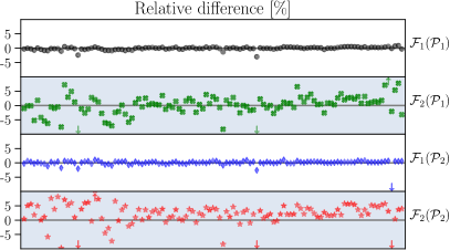
Figure 3: Relative differences between the measured $f_{\rm mer}^{h}$ frequencies and the corresponding values from the fit. Different rows refer to the four different possibilities of applying the fitting function $\mathcal{F}_{i}$ to the data pipeline $\mathcal{P}_{i}$ with $i=1,2$; arrows indicate relative differences above $10\%$. Note how the new fitting function and pipeline, i.e., $\mathcal{F}_{1}(\mathcal{P}_{1})$, provide errors that are about four times smaller.

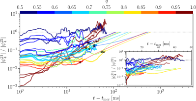
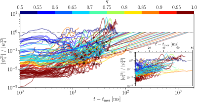
Figure 4: Evolution of the ratio of the two main GW modes $|\psi_{4}^{21}|/|\psi_{4}^{22}|$, with the left panel showing a selected set of binaries to highlight the behaviour for different mass ratios (colour code) and the right one reporting all of the binaries. Black dotted horizontal lines are used to mark the position when the two modes have equal amplitudes, while straight coloured lines report a linear extrapolation after averaging the last $5\,{\rm ms}$ of the evolution; note that the large majority of binaries exhibits a growing trend that is maintained throughout the computed evolution.

5 Secular GW emission

The last point we cover regards the relative strengths of the $\ell=2,m=2$ and $\ell=2,m=1$ GW modes. The importance of the latter was first pointed out in (Paschalidis et al., 2015; Lehner et al., 2016a) and is produced by corresponding asymmetries in the rest-mass density. The emergence of an $m=1$ deformation is well-known to occur in isolated stars (Chandrasekhar, 1969; Shibata et al., 2000; Baiotti et al., 2007; Franci et al., 2013; Löffler et al., 2015) that have a sufficiently large amount of rotational kinetic energy $T$ and emerges when the ratio $T/|W|$, where $W$ is the gravitational binding energy, exceeds a certain threshold (in a systematic analysis, Baiotti et al., 2007, have shown that this happens for $T/|W|\gtrsim 0.25$). In such stars, the $m=1$ mode in the rest-mass density would grow exponentially reaching equipartition with the $m=2$ mode, and, subsequently, represent the largest deformation. A similar phenomenology seems to be present also for the postmerger remnant, as already hinted in (Papenfort et al., 2022), but as shown more clearly by the numerous binaries considered here. Figure 4 reports the evolution of the ratio of the GW amplitudes in the two modes $|\psi_{4}^{21}|/|\psi_{4}^{22}|$, with the left panel showing a selected set of binaries and with the right panel reporting all binaries (the raw timeseries are smoothed over a window $\Delta t=0.5\,{\rm ms}$). While only a few binaries in the sample reach $|\psi_{4}^{21}|/|\psi_{4}^{22}|=1$ within the simulated time, the large majority exhibits a trend that we try to capture by extrapolating linearly in time after averaging the last $5\,{\rm ms}$ of the evolution. Using a colour code to distinguish binaries with different $q$, it becomes clear that the initial strength of the $m=1$ mode is inversely proportional to the mass ratio, so that for an extremely asymmetric binary, i.e., $q\lesssim 0.6$, $|\psi_{4}^{21}|/|\psi_{4}^{22}|$ can be more than two orders of magnitude larger than for equal-mass binaries. At the same time, the initial mode-amplitude ratio does not depend on the merger dimensionless spin (Papenfort et al., 2022). Unsurprisingly, a similar behaviour can be observed when computing the signal-to-noise (SNR) ratio in the $m=2$ and $m=1$ modes. Specifically, by computing a time-windowed SNR ratio we can quantify the growing contribution of the subdominant mode in a similar fashion to estimates given by (Lehner et al., 2016b) and find that its increases to $\simeq\mathcal{O}(1)$ if the $m=1$ is not suppressed (see SM for details).

If confirmed by systematic, long-term evolutions, this finding would change the standard picture in which the largest signal in the BNS postmerger is to be expected at the $f_{2}$ frequency. Rather, the trend reported here suggests that the most powerful feature in the PSD for long-lived HMNSs may actually appear at a frequency $\simeq\tfrac{1}{2}f_{2}$. Because this falls in a more favourable region of the detectors sensitivities, and assuming a detection angle not favouring either of the modes, the corresponding signal-to-noise ratio will grow proportionally to the ratio between detectors noise at $\tfrac{1}{2}f_{2}$ and $f_{2}$, hence by a factor of $\sim 2$ for LIGO or Virgo.

While promising, this prospect should be accompanied by some caveats. First, it is possible that the growth rate may be weaker than the one estimated here. Second, the extrapolation assumes that the HMNS will not collapse to a black hole before reaching $|\psi_{4}^{21}|/|\psi_{4}^{22}|\sim 1$ and while this is likely for soft EOSs and low-mass binaries, it may not happen if the EOS is stiff and the binary massive. Third, all binaries in our sample have zero deformation. A robust conclusion that can be inferred from the results shown in Fig. 4 is that remnants with a long lifetime, as it was likely the case for GW170817 (Rezzolla et al., 2018; Gill et al., 2019; Murguia-Berthier et al., 2021), will reasonably have the $\ell=2,m=1$ as the least-damped mode. Hence, considerable spectral power should be present at frequencies $\frac{1}{2}f_{2}$ and $f_{2}$, with the main strain amplitudes in a ratio $|h^{21}|/|h^{22}|\sim 0.1-1$ for generic orientations (e.g., for an inclination of $2\arctan(1/2)\sim 53^{\circ}$ two modes have the same spin-weighted spherical-harmonics coefficients).

6 Conclusion

Leveraging on a rich literature developed over the last ten years on this subject, we have considered again the spectral properties of the signal when computed in terms of the Weyl scalar $\psi_{4}$ rather than in terms of the GW strain $h_{+,\times}$. Exploiting the better behaviour of $\psi_{4}$, we were able to highlight three novel features that can be used to better infer physical information from the detected signal.

First, by employing a large number of simulations spanning a considerable set of EOSs and mass ratios, we have shown the existence of a new instantaneous frequency, $f^{\psi_{4}}_{0}$, that can be associated with the instant of quasi time-symmetry in the postmerger dynamics. This corresponds to when the stellar cores in the merger remnant have reached their minimum separation and are about to bounce-off each other. Just like other spectral frequencies of the BNS GW signal, $f^{\psi_{4}}_{0}$ also follows a quasi-universal behaviour as a function of the tidal deformability $\kappa_{2}^{{}_{T}}$ and of the binary mass ratio $q$, for which we provide a simple and yet accurate analytical expression. Second, we have obtained a new quasi-universal relation for the merger frequency $f^{h}_{\rm mer}$ as a function of $\kappa_{2}^{{}_{T}}$ and $q$. The new expression not only requires a smaller number of fitting coefficients than alternative expressions in the literature, but it also provides a more accurate description of the data, with a residual error that is four times smaller on average. Finally, we have pointed out the evidence that the $\ell=2,m=1$ could become the most powerful GW mode on sufficiently long timescales, with strain amplitudes for the dominant modes that are in a ratio $|h^{21}|/|h^{22}|\sim 0.1-1$. Should this mode not be suppressed by the collapse of the HMNS to a black hole or by other dissipative effects such as magnetic fields, considerable spectral power should be present at frequencies $\frac{1}{2}f_{2}$, where it could be detected in conditions of smaller signal-to-noise ratios or by third-generation detectors.

The results presented here can be improved by enlarging the number of BNS simulations considered, by increasing the variance in the microphysical description (e.g., including simulations with magnetic fields and neutrino transport), by performing additional long-term evolutions, and by extending the fitting approach to binaries with spins and eccentricity. We will explore these extensions in future work.

Data policy. The relevant data that supports the findings of this paper is available from the first author and can be shared upon a reasonable request.

We thank K. Chakravarti, K. Takami, C. Ecker, and C. Musolino for useful input and discussions. Support comes from the State of Hesse within the Research Cluster ELEMENTS (Project ID 500/10.006). LR acknowledges funding by the ERC Advanced Grant “JETSET: Launching, propagation and emission of relativistic jets from binary mergers and across mass scales” (Grant No. 884631). The simulations from which parts of the used data are derived were performed on HPE Apollo HAWK at the High Performance Computing Center Stuttgart (HLRS) under the grants BNSMIC and BBHDISKS, and on SuperMUC at the Leibniz Supercomputing Centre.

Supplemental Material

Toy-model analogy

Although it is possible to characterise the new spectral feature $f_{0}$ simply in terms of the instantaneous GW frequency at the time $t^{\psi_{4}}_{0}$ at which the Weyl scalar has its first minimum, it is more interesting to associate with this definition also a physical interpretation. As mentioned in the main text, $t^{\psi_{4}}_{0}$ effectively corresponds to when the two stellar cores have reached the minimum separation and are about to bounce-off each other. At this instant, the radial velocity of the two stellar cores and the angular velocity of the HMNS has a minimum, so that the corresponding amplitude of $\psi_{4}$ has a minimum and instantaneous GW frequency a local maximum.

To illustrate this behaviour, we employ the toy model developed in Takami et al. (2015) (and also employed in other studies, e.g.,  Ellis et al. (2018); Lucca et al. (2021)) to describe the dynamics of the postmerger remnant and which consists of an axisymmetric disk rotating rapidly at a given angular frequency, say $\Omega_{2}$, to which two spheres reproducing the two stellar cores are connected but are also free to oscillate via a spring that connects them (see Fig. 17 Takami et al. (2015)). In such a system, the two spheres will either approach each other, decreasing the moment of inertia of the system, or move away from each other, increasing the moment of inertia. Because the total angular momentum is essentially conserved, the system’s angular frequency will vary between a minimum value $\Omega_{1}$ (corresponding to the time when the two spheres are at the largest separation) and a maximum value $\Omega_{3}$ (corresponding to the time when the two spheres are at the smallest separation). Overall, the mechanical toy model will rotate with an angular frequency that is a function of time and bounded by $\Omega_{1}$ and $\Omega_{3}$, where more time is spent and hence more spectral power is accumulated. If a damping is introduced, the excursion of the oscillations between the spheres will decrease over time and eventually stop; when this happens, the toy model will simply rotate at the frequency $\Omega_{2}$, as does the HMNS after the transient period and before other deformations (e.g., the $\ell=2,m=1$ mode) affect it.

The Lagrangian of the toy model can be found in Takami et al. (2014) and from it it is possible to derive the differential equation for the radial displacement $r(t)$

$$\ddot{r}+\frac{4k(r-r_{0})}{m}-\Bigg{[}\frac{c_{1}}{r^{2}+MR^{2}/(2m)}\Bigg{]}^{2}r+\frac{2br}{m}=0\,,$$ (1)

where $M$ and $m$ are the masses of the disc and of the spheres, $R$ is the radius of the disc, $c_{1}$ an integration constant related to the total angular momentum, $r_{0}$ the natural displacement of mass and $b$ is responsible for dissipative effects. The dissipation due to the emission of GWs and which results in the two spheres getting closer to one another with time and with a decreasing radial displacement is introduced by varying the natural displacement $r_{0}$ via via an exponential function $\exp({-{t}/{\tau}})$ with a suitably chosen relaxation time $\tau$. Note that this modification carries straight from the Lagrangian to the final ODE without additional time derivatives, as it is present in the derivative of the Lagrangian with respect to the canonical coordinate $r(t)$ and not its conjugate.

The system is sufficiently simple that it is possible to compute the GW amplitude and frequency derived from the quadrupole formula so that the strain components read

$$h_{+}=\frac{2m}{d}[\{\dot{r}^{2}+r(\ddot{r}-2r\Omega^{2})\}\cos(2\varphi)-r(4\dot{r}\Omega+r\dot{\Omega})\sin(2\varphi)~{}]\,,$$

$$h_{\times}=\frac{2m}{d}[\{\dot{r}^{2}+r(\ddot{r}-2r\Omega^{2})\}\sin(2\varphi)+r(4\dot{r}\Omega+r\dot{\Omega})\cos(2\varphi)~{}]\,,$$

with $d$ the distance from the source to the detector. The $\psi_{4}$ polarisations are obtained by differentiating twice with respect to time. Introducing the abbreviations $A\,\coloneqq\dot{r}^{2}+r(\ddot{r}-2r\Omega^{2})$ and $B\,\coloneqq r(4\dot{r}\Omega+r\dot{\Omega})$, as well as recalling that $\Omega(t)=\dot{\varphi}(t)$ we write them now explicitly

$$\psi_{4,+}=\frac{2m}{d}[-\sin(2\varphi)\{4\dot{\varphi}(\dot{A}-B\dot{\varphi})+\ddot{B}+2A\ddot{\varphi}\}+\cos(2\varphi)\{-4\dot{\varphi}(\dot{B}+A\dot{\varphi})+\ddot{A}-2B\ddot{\varphi}\}~{}]\,,$$

$$\psi_{4,\times}=-\frac{2m}{d}[\cos(2\varphi)\{4\dot{\varphi}(\dot{A}-B\dot{\varphi})+\ddot{B}+2A\ddot{\varphi}\}+\sin(2\varphi)\{-4\dot{\varphi}(\dot{B}+A\dot{\varphi})+\ddot{A}-2B\ddot{\varphi}\}~{}]\,,$$

where $\psi_{4,+}:=\partial^{2}_{t}h_{+}$ and $\psi_{4,\times}:=\partial^{2}_{t}h_{\times}$.

The amplitude and the instantaneous frequency of the signal are calculated using the usual definitions

$$|\psi_{4}(t)| \coloneqq \sqrt{\psi_{4,\times}^{2}(t)+\psi_{4,+}^{2}(t)}\,,$$ (2)

$$f_{\rm GW}^{\psi_{4}}(t) \coloneqq \frac{1}{2\pi}\frac{d}{dt}\arctan\left(\frac{\psi_{4,\times}(t)}{\psi_{4,+}(t)}\right)\,.$$ (3)

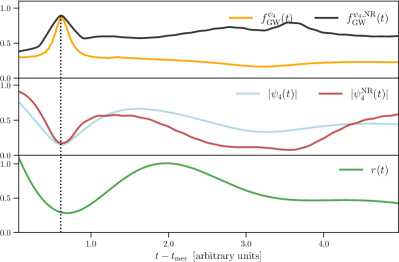
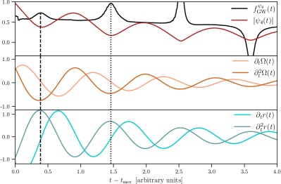
Figure 5: Solution of the toy model for a representative set of parameters. The left panel reports the GW frequency (top row) from the toy model and from an actual simulation (marked by the index “NR”), the GW amplitudes (middle row) and the radial displacement $r(t)$ (bottom row). The right panel shows instead the relation between the GW quantities and other dynamical quantities of the toy model, such as the time derivatives of the angular velocity and of the radial displacement. Note that the GW frequencies and amplitudes are anti-correlated and the minimum in the radial displacement at $t^{\psi_{4}}_{0}$ corresponds to the maximum frequency $f^{\psi_{4}}_{0}$ and minimum amplitude. Also, the minima of the amplitude (maxima of the frequency) correspond to moments in time when the angular frequency $\Omega$ attains a local maximum, and the radial displacement a local minimum.

The rather lengthy final expressions read:

$$\frac{d}{2m}|\psi_{4}(t)| = \big{[}~{}4\sin(2\varphi)\dot{A}\dot{\varphi}+4\cos(2\varphi)\dot{B}\dot{\varphi}+4A\cos(2\varphi)\dot{\varphi}^{2}-4B\sin(2\varphi)\dot{\varphi}^{2}-\cos(2\varphi)\ddot{A}+\sin(2\varphi)\ddot{B}$$ (4)

$$+2B\cos(2\varphi)\ddot{\varphi}+2A\sin(2\varphi)\ddot{\varphi}~{}\big{]}^{2}+\big{[}~{}4\cos(2\varphi)\dot{A}\dot{\varphi}-4\sin(2\varphi)\dot{B}\dot{\varphi}-4B\cos(2\varphi)\dot{\varphi}^{2}-4A\sin(2\varphi)\dot{\varphi}^{2}$$

$$+\sin(2\varphi)\ddot{A}+\cos(2\varphi)\ddot{B}+2A\cos(2\varphi)\ddot{\varphi}-2B\sin(2\varphi)\ddot{\varphi}~{}\big{]}^{2},$$

$$2\pi\frac{f_{\rm GW}^{\psi_{4}}}{F^{\psi_{4}}} = 48\dot{A}^{2}\dot{\varphi}^{3}+48\dot{B}^{2}\dot{\varphi}^{3}+32A^{2}\dot{\varphi}^{5}+32B^{2}\dot{\varphi}^{5}-32A\dot{\varphi}^{3}\ddot{A}+6\dot{\varphi}\ddot{A}^{2}-32B\dot{\varphi}^{3}\ddot{B}+6\dot{\varphi}\ddot{B}^{2}-24B\dot{\varphi}\ddot{A}\ddot{\varphi}$$ (5)

$$+24A\dot{\varphi}\ddot{B}\ddot{\varphi}+24A^{2}\dot{\varphi}\ddot{\varphi}^{2}+24B^{2}\dot{\varphi}\ddot{\varphi}^{2}+4B\dot{\varphi}^{2}\dddot{A}-\ddot{B}\dddot{A}-2A\ddot{\varphi}\dddot{A}-4A\dot{\varphi}^{2}\dddot{B}+\ddot{A}\dddot{B}-2B\ddot{\varphi}\dddot{B}$$

$$+2\big{(}-4A^{2}\dot{\varphi}^{2}+A\ddot{A}+B(-4B\dot{\varphi}^{2}+\ddot{B})\big{)}\dddot{\varphi}+2\dot{B}\big{(}3\ddot{B}\ddot{\varphi}+6\dot{\varphi}^{2}(-3\ddot{A}+4B\ddot{\varphi})-2\dot{\varphi}\dddot{B}+A(40\ddddot{\varphi}+6\ddot{\varphi}^{2}-4\dot{\varphi}\dddot{\varphi})\big{)}$$

$$+\dot{A}\big{(}6\ddot{A}\ddot{\varphi}+12\dot{\varphi}^{2}(3\ddot{B}+4A\ddot{\varphi})-4\dot{\varphi}\dddot{A}-4B(20\dot{\varphi}^{4}+3\ddot{\varphi}^{2}-2\dot{\varphi}\dddot{\varphi})\big{)},$$

$$\frac{-1}{F^{\psi_{4}}} := 16\dot{A}^{2}\dot{\varphi}^{2}+16\dot{B}^{2}\dot{\varphi}^{2}+16A^{2}\dot{\varphi}^{4}+16B^{2}\dot{\varphi}^{4}-8A\dot{\varphi}^{2}\ddot{A}+\ddot{A}^{2}-8B\dot{\varphi}^{2}\ddot{B}+\ddot{B}^{2}+4(-B\ddot{A}+A\ddot{B})\ddot{\varphi}$$ (6)

$$+4(A^{2}+B^{2})\ddot{\varphi}^{2}+8\dot{A}\dot{\varphi}(-4B\dot{\varphi}^{2}+\ddot{B}+2A\ddot{\varphi})+8\dot{B}\dot{\varphi}(4A\dot{\varphi}^{2}-\ddot{A}+2B\ddot{\varphi})\,.$$

Figure 5 reports the solution of the system when considering the following set of representative parameters: $M=m=10$, $k=0.2$, $b=0.25$, $c_{1}=25$, $R=22$, $r_{0}=5$, $\dot{r}_{0}=0.01$, $\tau=1000$. More specifically, the left panel reports the GW frequency (top row) as computed from the toy model and from an actual simulation (marked by the index “NR”), the corresponding GW amplitudes (middle row) and the radial displacement $r(t)$ (bottom row). Note how the GW frequencies and amplitudes are anti-correlated and the minimum in the radial displacement at $t^{\psi_{4}}_{0}$ corresponds to the maximum frequency, i.e., $f^{\psi_{4}}_{0}$, and minimum amplitude, as expected in a condition of quasi time-symmetry (in the toy model $f^{h}_{0}$ is actually a local minimum of $f^{h}_{\rm GW}(t)$, a case often found in NR data). The right panel of Fig. 5, on the other hand, is used to show the relation between the GW quantities of the toy model and other dynamical quantities such as the time derivatives of the angular velocity, $\partial_{t}\Omega(t)$ and $\partial^{2}_{t}\Omega(t)$, and of the radial displacement, $\partial_{t}r(t)$ and $\partial^{2}_{t}r(t)$ (the top row of the right panel contains the same information as in the top and middle row of the left panel). It is clear that for the first few oscillations the minima of the amplitude (maxima of the frequency) correspond to moments in time when the angular frequency $\Omega$ attains a local maximum, and the radial displacement a local minimum.

We find it rather remarkable that the model originally developed to provide justification for the dominant postmerger frequency can be used to mimic the presence of the $f_{0}$ frequency with no additional adjustments, appearing as a result of chosen parameters and initial conditions. Finally, while we do not consider it here, it would be useful to generalise the model to admit unequal sphere masses, i.e., $m/M<1$, and assess the impact it has on the $f_{0}$ frequency and on the evolution of the $m=2$ and $m=1$ modes.

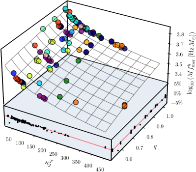
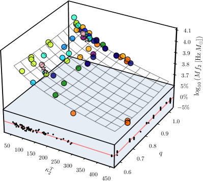
Figure 6: The same as in Fig. $2$ in the main text but for the GW frequencies $f^{h}_{\rm mer}$ and $f_{2}$. Note how $\mathcal{F}_{1}$ is equally accurate in modelling other frequencies, also when obtained from the strain as in the case for $f^{h}_{\rm mer}$ and $f_{2}$.

On the effectiveness of the fit

To illustrate effectiveness of the fitting functional form $\mathcal{F}_{1}$ in capturing the spectral properties of the signal in a quasi-universal manner, we report in Fig. $2$ the same 3D representation as of the GW frequencies shown in Fig. $2$ but for the GW frequencies $f^{h}_{\rm mer}$ and $f_{2}$; note that $f^{h}_{\rm mer}$ is referred to as $f_{\rm max}$ in Takami et al. (2014); Rezzolla & Takami (2016) and that the $f_{2}$ frequency corresponds to the peak of the PSD computed using the definition in Tootle et al. (2022), with the time integration encompassing the full GW signal. Clearly, the fitting function $\mathcal{F}_{1}$ is equally accurate in modelling other frequencies, quite independently of whether they have been computed from the Weyl scalar or from the GW strain, as it is as it is the case for $f^{h}_{\rm mer}$ and $f_{2}$. We also note that the equal-mass limit of the fitting function $\mathcal{F}_{1}$ for the frequency $f^{h}_{\rm mer}$, recovers quite accurately the simpler fit examined in Takami et al. (2014) which expressed the merger frequency as a first-order expression of the tidal deformability $f^{h}_{\rm mer}=a_{0}+b({\kappa_{2}^{{}_{T}}})^{{1}/{5}}$. When setting $q=1$ and $n={1}/{5}$ in $\mathcal{F}_{1}$, we obtain $b=b_{0}+b_{1}+b_{2}=-0.199$ (cf., Table 1), thus resulting in a relative difference that is $\lesssim 2\%$ with respect to the value $b=-0.195$ found in Takami et al. (2014). At the same time, we also note that the fit of $f^{h}_{\rm mer}$ is overall slightly better than that for $f^{\psi_{4}}_{\rm mer}$ (see Table 1); while we do not believe this to be statistically very significant, it may be due to the slightly larger range in which $f^{\psi_{4}}_{\rm mer}$ is measured.

The only exception to the remarkably good fit of the frequencies is found in the $f^{\psi_{4}}_{0}$ frequency, where a noticeable deviation from the trend is visible for binary systems with equal or very-unequal masses, regardless of the EOS employed (see lower part of the bottom-right panel of Fig. $2$). We attribute this decrease in accuracy to the already described difficulties of measuring this frequency using the $\psi_{4}$ GW signal, which are even more severe when using $|h|$. From a physical point of view, the moment of time symmetry corresponds to the time when the non-axisymmetric quadrupolar deformations of the HMNS are at a minimum, which leads to a severely suppressed GW signal (indeed the amplitude is at a minimum). This is particularly severe for binaries with $q\simeq 1$, where the $\ell=2,m=2$ deformation is the largest and is significantly suppressed at the moment of time-symmetry, and for binaries with $q\ll 1$, where the $\ell=2,m=2$ deformation is further decreased by the mass asymmetry. Notwithstanding these difficulties, relative fitting error for $f^{\psi_{4}}_{0}$ [i.e., $\max(\Delta f/f$)] is at most $4.2\%$ and only $1.4\%$ on average [i.e., $\langle|\Delta f|/f\rangle$].

Freq.	$a_{0}$	$b_{0}$	$b_{1}$	$b_{2}$	$n$	$\langle\Delta f/f\rangle$	$\max(\Delta f/f)$	$\chi^{2}$	$\chi^{2}_{\rm red}$	$R^{2}$
						$[\%]$	$[\%]$		$\times 10^{-3}$
$f^{\psi_{4}}_{\rm mer}$	$4.589$	$-0.581$	$\phantom{-}0.543$	$-0.236$	$0.20\phantom{{}^{\dagger}}$	$0.65$	$4.52$	$0.135$	$1.19$	$0.934$
$f^{h}_{\rm mer}$	$4.201$	$-0.330$	$\phantom{-}0.198$	$-0.067$	$0.20\phantom{{}^{\dagger}}$	$0.32$	$2.99$	$0.035$	$0.30$	$0.957$
$f^{\psi_{4}}_{\rm mer}$	$6.067$	$-2.142$	$\phantom{-}0.970$	$-0.410$	$0.07^{\dagger}$	$0.59$	$4.24$	$0.114$	$1.00$	$0.938$
$f^{h}_{\rm mer}$	$4.457$	$-0.578$	$\phantom{-}0.262$	$-0.087$	$0.14^{\dagger}$	$0.32$	$2.94$	$0.034$	$0.30$	$0.957$
$f^{\psi_{4}}_{0}$	$6.550$	$-2.099$	$\phantom{-}0.518$	$-0.304$	$0.06^{\dagger}$	$1.38$	$4.22$	$0.477$	$4.92$	$0.611$
$f_{2}$	$4.617$	$-0.170$	$-0.264$	$\phantom{-}0.160$	$0.20^{\dagger}$	$0.45$	$1.34$	$0.030$	$0.48$	$0.926$

Table 1: Best-fit values for the coefficients of the functional form $\mathcal{F}_{1}$. Also reported are the maximal and average relative difference, as well as the $\chi^{2}$, $\chi^{2}_{\rm{red}}$ and $R^{2}$ coefficients of the fit. Indicated with a $\dagger$ are the best-fit values of $n$ when this coefficient is constrained by the fit.

Growth of the SNR ratio

In the main text we have discussed how to use the amplitude ratio $|\psi_{4}^{21}|/|\psi_{4}^{22}|$ as an effective proxy for the relevance of the $m=1$ mode deformation. We next demonstrate that a clear correspondence exists between finding $|\psi_{4}^{21}|/|\psi_{4}^{22}|\sim 1$ and the ratio of the SNRs in the two modes. We start by recalling that given the power spectral density of the $m$-th mode of the GW strain decomposition $\tilde{h}_{m}(f)$ (such as the one presented in Fig. 1 for $m=2$) and a noise spectral density of the detector $S_{n}(f)$, the corresponding $m$-th SNR is defined as

$${\rm SNR}_{m=k}:=\left[\int_{0}^{\infty}4\frac{|\tilde{h}_{m=k}(f)|^{2}}{S_{n}(f)}df\right]^{\frac{1}{2}}\,.$$ (7)

Clearly, the ratio of the SNRs, ${\rm SNR}_{m=1}/{\rm SNR}_{m=2}$ and the rate at which it evolves depends on the time $t_{i}$ when the signal starts to be considered. Because there is no $m=1$ signal during the inspiral, the SNR ratio would be intrinsically dominated by the $m=2$ component of the signal if $t_{i}$ was chosen to be the time the signal entered the detector. Hence, to fairly assess the growing contribution of the $m=1$ mode, we compute a time-windowed SNR over a running window of width $\Delta T=5\,$ms. We should remark that this approach is logically and mathematically equivalent to what is done when computing spectrograms (see, e.g.,  The LIGO Scientific Collaboration & The Virgo Collaboration, 2017) and hence determines, at any given time, the characteristic frequency at which the GW is emitted. In essence, for any time $\bar{t}$, we compute the SNR as defined in Eq. (7), where the signal in the time domain is in the interval $t\in[\bar{t}-\Delta T/2,\bar{t}+\Delta T/2]$. This time-windowed SNR provides an “instantaneous” measure of the ability of a detector to measure a signal of given strength and is mathematically equivalent to what is routinely done when computing spectrograms in GW data analysis.

As demonstrated in Fig. 7, the SNR ratio computed in this way grows to be of $\mathcal{O}(1)$ at the same time when $|\psi_{4}^{21}|/|\psi_{4}^{22}|\simeq\mathcal{O}(1)$, thus supporting the effectiveness of the mode ratio in acting as a proxy for the SNR ratio. Finally, we note that the estimates provided in Fig. 7 are similar in spirit to the SNR estimates suggested by Lehner et al. (2016b). We stress that the results shown should not be interpreted as pointing out to a global-in-time dominance of the $m=1$ mode; rather, they suggest a an enhanced importance of this mode that is local-in-time and appears only long past the merger. When considering the full GW signal, the $m=2$ will always provide the largest contribution, by far.

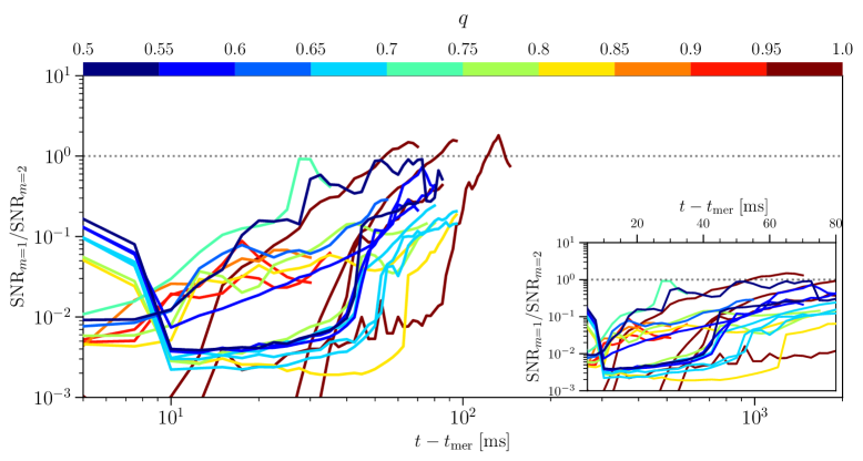
Figure 7: Instantaneous SNR ratio as computed for the selected set of configurations in Fig.$4$ of the main text, where the time-window has been chosen to be $\Delta T=5\,$ms. The detector’s sensitivity is based on the O3 observing run of LIGO and the angle of observation does not favour either of the modes. Note that ${\rm SNR}_{m=1}/{\rm SNR}_{m=2}\simeq\mathcal{O}(1)$ around the same time as $|\psi_{4}^{21}|/|\psi_{4}^{22}|\simeq\mathcal{O}(1)$.

References

- Alford et al. (2005) Alford, M., Braby, M., Paris, M., & Reddy, S. 2005, Astrophys. J., 629, 969, doi: 10.1086/430902
- Anderson et al. (2008) Anderson, M., Hirschmann, E. W., Lehner, L., et al. 2008, Phys. Rev. D, 77, 024006, doi: 10.1103/PhysRevD.77.024006
- Baiotti et al. (2007) Baiotti, L., De Pietri, R., Manca, G. M., & Rezzolla, L. 2007, Phys. Rev. D, 75, 044023, doi: 10.1103/PhysRevD.75.044023
- Baiotti et al. (2008) Baiotti, L., Giacomazzo, B., & Rezzolla, L. 2008, Phys. Rev. D, 78, 084033, doi: 10.1103/PhysRevD.78.084033
- Baiotti & Rezzolla (2017) Baiotti, L., & Rezzolla, L. 2017, Rept. Prog. Phys., 80, 096901, doi: 10.1088/1361-6633/aa67bb
- Bauswein et al. (2019) Bauswein, A., Bastian, N.-U. F., Blaschke, D. B., et al. 2019, Phys. Rev. Lett., 122, 061102, doi: 10.1103/PhysRevLett.122.061102
- Bauswein et al. (2019) Bauswein, A., Bastian, N.-U. F., Blaschke, D. B., et al. 2019, Physical Review Letters, 122, 061102, doi: 10.1103/PhysRevLett.122.061102
- Bauswein & Janka (2012) Bauswein, A., & Janka, H.-T. 2012, Phys. Rev. Lett., 108, 011101, doi: 10.1103/PhysRevLett.108.011101
- Bauswein & Stergioulas (2015) Bauswein, A., & Stergioulas, N. 2015, Phys. Rev. D, 91, 124056, doi: 10.1103/PhysRevD.91.124056
- Bauswein et al. (2016) Bauswein, A., Stergioulas, N., & Janka, H.-T. 2016, European Physical Journal A, 52, 56, doi: 10.1140/epja/i2016-16056-7
- Bernuzzi et al. (2014) Bernuzzi, S., Nagar, A., Balmelli, S., Dietrich, T., & Ujevic, M. 2014, Phys. Rev. Lett., 112, 201101, doi: 10.1103/PhysRevLett.112.201101
- Bishop & Rezzolla (2016) Bishop, N. T., & Rezzolla, L. 2016, Living Reviews in Relativity, 19, 2, doi: 10.1007/s41114-016-0001-9
- Bose et al. (2018) Bose, S., Chakravarti, K., Rezzolla, L., Sathyaprakash, B. S., & Takami, K. 2018, Phys. Rev. Lett., 120, 031102, doi: 10.1103/PhysRevLett.120.031102
- Bozzola (2021) Bozzola, G. 2021, The Journal of Open Source Software, 6, 3099, doi: 10.21105/joss.03099
- Breschi et al. (2022) Breschi, M., Bernuzzi, S., Chakravarti, K., et al. 2022, arXiv e-prints, arXiv:2205.09112, doi: 10.48550/arXiv.2205.09112
- Breschi et al. (2019) Breschi, M., Bernuzzi, S., Zappa, F., et al. 2019, Phys. Rev. D, 100, 104029, doi: 10.1103/PhysRevD.100.104029
- Calderon Bustillo et al. (2022) Calderon Bustillo, J., Wong, I. C. F., Sanchis-Gual, N., et al. 2022, arXiv e-prints, arXiv:2205.15029, doi: 10.48550/arXiv.2205.15029
- Camilletti et al. (2022) Camilletti, A., Chiesa, L., Ricigliano, G., et al. 2022, Mon. Not. R. Astron. Soc., 516, 4760, doi: 10.1093/mnras/stac2333
- Chabanov et al. (2023) Chabanov, M., Tootle, S. D., Most, E. R., & Rezzolla, L. 2023, Astrophys. J. Lett., 945, L14, doi: 10.3847/2041-8213/acbbc5
- Chandrasekhar (1969) Chandrasekhar, S. 1969, Ellipsoidal figures of equilibrium
- Ciolfi et al. (2019) Ciolfi, R., Kastaun, W., Kalinani, J. V., & Giacomazzo, B. 2019, Phys. Rev. D, 100, 023005, doi: 10.1103/PhysRevD.100.023005
- De Pietri et al. (2019) De Pietri, R., Drago, A., Feo, A., et al. 2019, Astrophys. J., 881, 122, doi: 10.3847/1538-4357/ab2fd0
- De Pietri et al. (2020) De Pietri, R., Feo, A., Font, J. A., et al. 2020, Phys. Rev. D, 101, 064052, doi: 10.1103/PhysRevD.101.064052
- Demircik et al. (2022) Demircik, T., Ecker, C., & Järvinen, M. 2022, Phys. Rev. X, 12, 041012, doi: 10.1103/PhysRevX.12.041012
- Dionysopoulou et al. (2013) Dionysopoulou, K., Alic, D., Palenzuela, C., Rezzolla, L., & Giacomazzo, B. 2013, Phys. Rev. D, 88, 044020, doi: 10.1103/PhysRevD.88.044020
- East et al. (2015) East, W. E., Paschalidis, V., & Pretorius, F. 2015, Astrophys. J. Lett., 807, L3, doi: 10.1088/2041-8205/807/1/L3
- East et al. (2019) East, W. E., Paschalidis, V., Pretorius, F., & Tsokaros, A. 2019, Phys. Rev. D, 100, 124042, doi: 10.1103/PhysRevD.100.124042
- Ellis et al. (2018) Ellis, J., Hütsi, G., Kannike, K., et al. 2018, Phys. Rev. D, 97, 123007, doi: 10.1103/PhysRevD.97.123007
- Espino et al. (2023) Espino, P. L., Prakash, A., Radice, D., & Logoteta, D. 2023, arXiv e-prints, arXiv:2301.03619, doi: 10.48550/arXiv.2301.03619
- Foucart et al. (2022) Foucart, F., Duez, M. D., Haas, R., et al. 2022, arXiv e-prints, arXiv:2210.05670, doi: 10.48550/arXiv.2210.05670
- Franci et al. (2013) Franci, L., De Pietri, R., Dionysopoulou, K., & Rezzolla, L. 2013, Phys. Rev. D, 88, 104028, doi: 10.1103/PhysRevD.88.104028
- Fujimoto et al. (2023) Fujimoto, Y., Fukushima, K., Hotokezaka, K., & Kyutoku, K. 2023, Phys. Rev. Lett., 130, 091404, doi: 10.1103/PhysRevLett.130.091404
- Gieg et al. (2019) Gieg, H., Dietrich, T., & Ujevic, M. 2019, arXiv e-prints, arXiv:1908.03135. https://arxiv.org/abs/1908.03135
- Gill et al. (2019) Gill, R., Nathanail, A., & Rezzolla, L. 2019, Astrophys. J., 876, 139, doi: 10.3847/1538-4357/ab16da
- Gonzalez et al. (2022) Gonzalez, A., Zappa, F., Breschi, M., et al. 2022, arXiv e-prints, arXiv:2210.16366, doi: 10.48550/arXiv.2210.16366
- Grandclement (2010) Grandclement, P. 2010, J. Comput. Phys., 229, 3334, doi: 10.1016/j.jcp.2010.01.005
- Haas & et al. (2020) Haas, R., & et al. 2020, The Einstein Toolkit, The ”DeWitt-Morette” release, ET_2020_11, Zenodo, doi: 10.5281/zenodo.4298887
- Hotokezaka et al. (2011) Hotokezaka, K., Kyutoku, K., Okawa, H., Shibata, M., & Kiuchi, K. 2011, Phys. Rev. D, 83, 124008, doi: 10.1103/PhysRevD.83.124008
- Kiuchi et al. (2015) Kiuchi, K., Cerdá-Durán, P., Kyutoku, K., Sekiguchi, Y., & Shibata, M. 2015, Phys. Rev. D, 92, 124034, doi: 10.1103/PhysRevD.92.124034
- Kiuchi et al. (2022) Kiuchi, K., Fujibayashi, S., Hayashi, K., et al. 2022, arXiv e-prints, arXiv:2211.07637, doi: 10.48550/arXiv.2211.07637
- Lehner et al. (2016a) Lehner, L., Liebling, S. L., Palenzuela, C., et al. 2016a, Classical and Quantum Gravity, 33, 184002, doi: 10.1088/0264-9381/33/18/184002
- Lehner et al. (2016b) Lehner, L., Liebling, S. L., Palenzuela, C., & Motl, P. M. 2016b, Phys. Rev. D, 94, 043003, doi: 10.1103/PhysRevD.94.043003
- Liebling et al. (2021) Liebling, S. L., Palenzuela, C., & Lehner, L. 2021, Classical and Quantum Gravity, 38, 115007, doi: 10.1088/1361-6382/abf898
- Liu et al. (2008) Liu, Y. T., Shapiro, S. L., Etienne, Z. B., & Taniguchi, K. 2008, Phys. Rev. D, 78, 024012, doi: 10.1103/PhysRevD.78.024012
- Löffler et al. (2015) Löffler, F., De Pietri, R., Feo, A., Maione, F., & Franci, L. 2015, Phys. Rev. D, 91, 064057, doi: 10.1103/PhysRevD.91.064057
- Logoteta, Domenico et al. (2021) Logoteta, Domenico, Perego, Albino, & Bombaci, Ignazio. 2021, A&A, 646, A55, doi: 10.1051/0004-6361/202039457
- Lucca et al. (2021) Lucca, M., Sagunski, L., Guercilena, F., & Fromm, C. M. 2021, Journal of High Energy Astrophysics, 29, 19, doi: 10.1016/j.jheap.2020.10.002
- Most et al. (2022) Most, E. R., Haber, A., Harris, S. P., et al. 2022, arXiv e-prints, arXiv:2207.00442. https://arxiv.org/abs/2207.00442
- Most et al. (2019) Most, E. R., Papenfort, L. J., Dexheimer, V., et al. 2019, Physical Review Letters, 122, 061101, doi: 10.1103/PhysRevLett.122.061101
- Most et al. (2019) Most, E. R., Papenfort, L. J., Dexheimer, V., et al. 2019, Phys. Rev. Lett., 122, 061101, doi: 10.1103/PhysRevLett.122.061101
- Most et al. (2019a) Most, E. R., Papenfort, L. J., & Rezzolla, L. 2019a, Mon. Not. R. Astron. Soc., 490, 3588, doi: 10.1093/mnras/stz2809
- Most et al. (2019b) Most, E. R., Papenfort, L. J., Tsokaros, A., & Rezzolla, L. 2019b, Astrophys. J., 884, 40, doi: 10.3847/1538-4357/ab3ebb
- Murguia-Berthier et al. (2021) Murguia-Berthier, A., Ramirez-Ruiz, E., De Colle, F., et al. 2021, Astrophys. J., 908, 152, doi: 10.3847/1538-4357/abd08e
- Oechslin & Janka (2007) Oechslin, R., & Janka, H.-T. 2007, Phys. Rev. Lett., 99, 121102, doi: 10.1103/PhysRevLett.99.121102
- Palenzuela et al. (2022) Palenzuela, C., Liebling, S., & Miñano, B. 2022, Phys. Rev. D, 105, 103020, doi: 10.1103/PhysRevD.105.103020
- Papenfort et al. (2022) Papenfort, L. J., Most, E. R., Tootle, S., & Rezzolla, L. 2022, Mon. Not. Roy. Astron. Soc., 513, 3646, doi: 10.1093/mnras/stac964
- Papenfort et al. (2021) Papenfort, L. J., Tootle, S. D., Grandclément, P., Most, E. R., & Rezzolla, L. 2021, Phys. Rev. D, 104, 024057, doi: 10.1103/PhysRevD.104.024057
- Paschalidis et al. (2015) Paschalidis, V., East, W. E., Pretorius, F., & Shapiro, S. L. 2015, Phys. Rev. D, 92, 121502, doi: 10.1103/PhysRevD.92.121502
- Prakash et al. (2021) Prakash, A., Radice, D., Logoteta, D., et al. 2021, Phys. Rev. D, 104, 083029, doi: 10.1103/PhysRevD.104.083029
- Radice et al. (2016) Radice, D., Bernuzzi, S., & Ott, C. D. 2016, Phys. Rev. D, 94, 064011, doi: 10.1103/PhysRevD.94.064011
- Radice et al. (2014a) Radice, D., Rezzolla, L., & Galeazzi, F. 2014a, Mon. Not. R. Astron. Soc. L., 437, L46, doi: 10.1093/mnrasl/slt137
- Radice et al. (2014b) —. 2014b, Class. Quantum Grav., 31, 075012, doi: 10.1088/0264-9381/31/7/075012
- Raithel & Most (2022) Raithel, C. A., & Most, E. R. 2022, Astrophys. J. Lett., 933, L39, doi: 10.3847/2041-8213/ac7c75
- Read et al. (2013) Read, J. S., Baiotti, L., Creighton, J. D. E., et al. 2013, Phys. Rev. D, 88, 044042, doi: 10.1103/PhysRevD.88.044042
- Rezzolla et al. (2011) Rezzolla, L., Giacomazzo, B., Baiotti, L., et al. 2011, Astrophys. J. Letters, 732, L6, doi: 10.1088/2041-8205/732/1/L6
- Rezzolla et al. (2018) Rezzolla, L., Most, E. R., & Weih, L. R. 2018, Astrophys. J. Lett., 852, L25, doi: 10.3847/2041-8213/aaa401
- Rezzolla & Takami (2016) Rezzolla, L., & Takami, K. 2016, Phys. Rev. D, 93, 124051, doi: 10.1103/PhysRevD.93.124051
- Schnetter et al. (2004) Schnetter, E., Hawley, S. H., & Hawke, I. 2004, Classical and Quantum Gravity, 21, 1465, doi: 10.1088/0264-9381/21/6/014
- Shibata et al. (2000) Shibata, M., Baumgarte, T. W., & Shapiro, S. L. 2000, Astrophys. J., 542, 453, doi: 10.1086/309525
- Shibata et al. (2005) Shibata, M., Taniguchi, K., & Uryū, K. 2005, Phys. Rev. D, 71, 084021, doi: 10.1103/PhysRevD.71.084021
- Sun et al. (2022) Sun, L., Ruiz, M., Shapiro, S. L., & Tsokaros, A. 2022, Phys. Rev. D, 105, 104028, doi: 10.1103/PhysRevD.105.104028
- Takami et al. (2014) Takami, K., Rezzolla, L., & Baiotti, L. 2014, Phys. Rev. Lett., 113, 091104, doi: 10.1103/PhysRevLett.113.091104
- Takami et al. (2015) —. 2015, Phys. Rev. D, 91, 064001, doi: 10.1103/PhysRevD.91.064001
- The CoRe Collaboration (2022) The CoRe Collaboration. 2022, core-watpy, 0.1.1. http://www.computational-relativity.org/
- The LIGO Scientific Collaboration & The Virgo Collaboration (2017) The LIGO Scientific Collaboration, & The Virgo Collaboration. 2017, Phys. Rev. Lett., 119, 161101, doi: 10.1103/PhysRevLett.119.161101
- Tootle et al. (2022) Tootle, S., Ecker, C., Topolski, K., et al. 2022, SciPost Phys., 13, 109, doi: 10.21468/SciPostPhys.13.5.109
- Tootle et al. (2021) Tootle, S. D., Papenfort, L. J., Most, E. R., & Rezzolla, L. 2021, Astrophys. J. Lett., 922, L19, doi: 10.3847/2041-8213/ac350d
- Ujevic et al. (2023) Ujevic, M., Gieg, H., Schianchi, F., et al. 2023, Phys. Rev. D, 107, 024025, doi: 10.1103/PhysRevD.107.024025
- Weih et al. (2020) Weih, L. R., Hanauske, M., & Rezzolla, L. 2020, Phys. Rev. Lett., 124, 171103, doi: 10.1103/PhysRevLett.124.171103
- Weih et al. (2020) Weih, L. R., Hanauske, M., & Rezzolla, L. 2020, Phys. Rev. Lett., 124, 171103, doi: 10.1103/PhysRevLett.124.171103
- Wolfram Research (2020) Wolfram Research, I. 2020, Mathematica, Version 12.1. https://www.wolfram.com/mathematica
- Zappa et al. (2023) Zappa, F., Bernuzzi, S., Radice, D., & Perego, A. 2023, Mon. Not. R. Astron. Soc., 520, 1481, doi: 10.1093/mnras/stad107