Superconductivity induced by strong electron-exciton coupling in doped atomically thin semiconductor heterostructures

Abstract

We study a mechanism to induce superconductivity in atomically thin semiconductors where excitons mediate an effective attraction between electrons. Our model includes interaction effects beyond the paradigm of phonon-mediated superconductivity and connects to the well-established limits of Bose and Fermi polarons. By accounting for the strong-coupling physics of trions, we find that the effective electron-exciton interaction develops a strong frequency and momentum dependence accompanied by the system undergoing an emerging BCS-BEC crossover from weakly bound $s$-wave Cooper pairs to a superfluid of bipolarons. Even at strong-coupling the bipolarons remain relatively light, resulting in critical temperatures of up to 10% of the Fermi temperature. This renders heterostructures of two-dimensional materials a promising candidate to realize superconductivity at high critical temperatures set by electron doping and trion binding energies.

In the past decade van der Waals materials have been shown to host a plethora of quantum phases of matter ranging from Mott and Wigner crystals [1, 2, 3, 4], the anomalous quantum Hall effect [5, 6, 7, 8], chiral edge states [9] and Chern insulators [10] to interaction-driven insulators [11]. Following the observation of unconventional superconductivity in NbSe2 monolayers [12], the discovery of superconductivity in magic-angle graphene [13, 14] and twisted bilayers of atomically thin semiconductors [15] have advanced van der Waals materials as a platform to realize novel forms of superconductivity.

The existence of strongly bound excitons in transition metal dichalcogenides (TMD) [16] has inspired studies exploring new routes to superconductivity. Recently, repulsive pairing mechanisms in twisted Moiré materials came into focus [17, 18, 19, 20, 21, 22, 23]. In this setting flat bands limit Fermi energies and thus the critical transition temperature. In absence of flat bands, theoretical works have explored exciton-mediated interactions between electrons analogous to the phonon-exchange in conventional BCS theory [24, 25, 26, 27, 28]. However, TMDs feature an exciton-electron coupling that is strong enough to feature exciton-electron bound states, trions, that remain stable up to room temperature [16], which cannot be captured by previously employed Fröhlich-type models [24, 25, 26, 27, 28]. Including this non-perturbative pairing physics in theoretical models has remained a central challenge, and the question how trion formation impacts superconductivity has been left unanswered.

In this letter, we present a theory of boson-induced superconductivity which incorporates the strong-coupling physics of the Bose-Fermi mixtures [29, 30, 31, 32, 33, 34] comprised of excitons and electrons. Our work does not rely on flat bands and applies to heterostructures of van der Waals materials where electrons interact with excitons in separated layers. We account for trion formation by considering beyond-linear electron-exciton coupling terms that extend the Fröhlich paradigm of electron-phonon exchange [35, 36]. As a result we find that the effective exciton-electron vertex becomes strongly retarded and non-local leading to strong dressing of electrons by the excitonic background. As the doping level in the TMD is tuned, the mutual dressing of electrons and excitons leads to an emergent crossover from a weak-coupling BCS superconductor into a superfluid state of bipolarons, akin to the BCS-BEC crossover observed in cold atoms [37, 38, 39, 40, 41, 42, 43, 44, 45, 46, 47, 48, 49, 50, 51, 52, 53]. Remarkably, we find the bipolarons to remain relatively light, facilitating the transition temperature to reach values of up to 10 % of the Fermi temperature. The physics of a BCS-BEC crossover emerging from mediated interactions complements the direct interaction mechanism in cold atoms and opens perspectives to reach high transition temperatures in van der Waals materials.

Model and Method.— We start from a two-dimensional Fermi gas of electrons ($\hat{c}_{\uparrow\mathbf{p}}$, $\hat{c}_{\downarrow\mathbf{p}}$) in absence of a magnetic field. The electrons interact with long-lived interlayer excitons in a spatially separated heterobilayer which could be realized in a MX₂-WX₂-MX’₂ heterostructure (X, X’ label chalcogen atoms) shown in Fig. 1(a). Electron tunneling between the top layers is fully suppressed by a large layer separation $d_{B}>d_{A}$ enabling $s$-wave pairing between electrons in the top layer. Gating can be employed to allow for doping of layer 3 in presence of a long-lived interlayer-(12) exciton. Since interlayer-(12) exciton energies for vanishing separation of the lower TMD layers 1 and 2 would be in the range $100$ to $150$ meV [54], Fermi energies of around $30$ meV in the TMD layer 3 would be possible. Importantly, due to the dipolar character of the system, the interlayer-(123) trion can have a substantial binding energy $\epsilon_{T}\sim 30$ meV comparable with the Fermi energy which brings the system into the strong coupling regime. We also emphasize that the generation of interlayer excitons need not require optical excitation [55, 56]. The interaction between electrons and the interlayer excitons, described by operators $\hat{X}^{\dagger}_{\mathbf{p}}$, and can be modelled by an attractive contact interaction of strength $g$ which can be directly related to the trion energy $\epsilon_{T}$ [57, 58]. In experiments the value of $\epsilon_{T}$ could for instance be tuned by changing the thickness of the hBN layer separating TMD layers 2 and 3, or using dielectric engineering [59, 60, 16]. The corresponding Hamiltonian is given by

$$\hat{H} =\sum_{\sigma=\uparrow,\downarrow}\sum_{\mathbf{k}}\epsilon^{c}_{\mathbf{k}}\hat{c}^{\dagger}_{\sigma\mathbf{k}}\hat{c}^{\phantom{\dagger}}_{\sigma\mathbf{k}}+\sum_{\mathbf{k}}\epsilon^{X}_{\mathbf{k}}\hat{X}^{\dagger}_{\mathbf{k}}\hat{X}^{\phantom{\dagger}}_{\mathbf{k}}$$

$$+\frac{g\sqrt{n_{0}}}{\sqrt{A}}\sum_{\sigma=\uparrow,\downarrow}\sum_{\mathbf{k}\mathbf{q}}\hat{c}^{\dagger}_{\sigma\mathbf{k}+\mathbf{q}}\hat{c}^{\phantom{\dagger}}_{\sigma\mathbf{k}}(\hat{X}^{\dagger}_{\mathbf{q}}+\hat{X}^{\phantom{\dagger}}_{-\mathbf{q}})$$

$$+\frac{g}{A}\sum_{\sigma=\uparrow,\downarrow}\sum_{\mathbf{k}\mathbf{k}^{\prime}\mathbf{q}}\hat{c}^{\dagger}_{\sigma\mathbf{k}+\mathbf{q}}\hat{c}^{\phantom{\dagger}}_{\sigma\mathbf{k}}\hat{X}^{\dagger}_{\mathbf{k}^{\prime}-\mathbf{q}}\hat{X}^{\phantom{\dagger}}_{\mathbf{k}^{\prime}},$$ (1)

with $A$ the system area. Assuming an effective mass approximation, the electron and exciton dispersion relations are $\epsilon^{c}_{\mathbf{k}}=\mathbf{k}^{2}/2m_{F}$ and $\epsilon^{X}_{\mathbf{k}}=\mathbf{k}^{2}/2m_{B}$. Although we investigate superconductivity in TMD, the Hamiltonian in Superconductivity induced by strong electron-exciton coupling in doped atomically thin semiconductor heterostructures may also be realized in ultracold atomic systems where the mass ratio between bosons and fermions can vary substantially. Considering the universal relevance of the model, we work at an equal mass ratio of excitons and electrons $m_{B}=m_{F}$. As the Fermi gas is spin-balanced, both components $\sigma=\uparrow,\downarrow$ are described by the Fermi wavevector $k_{F}=\sqrt{4\pi n_{F}}$ with density $n_{F}$. The Fermi level $\epsilon_{F}$ and temperature $T_{F}$ are given by $\epsilon_{F}=T_{F}=k_{F}^{2}/2m$. We set $\hbar=k_{B}=1$.

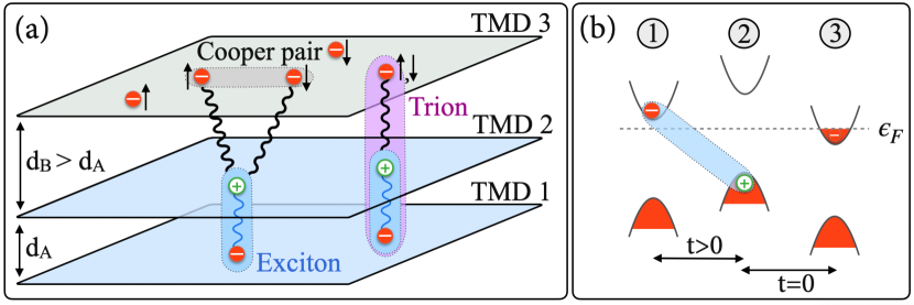
Figure 1: (a) Illustration of the TMD heterostructure. Charge carriers in the tunnel-coupled layers 1 and 2 form interlayer excitons which can bind with electrons in the spatially separated, tunnel-decoupled ($t=0$) top layer into deeply-bound trions. (b) Using gates the band alignment of the layers can be modified to allow doping of the third layer, while the interlayer (12) exciton remains stable. $\epsilon_{F}$ marks the Fermi level.

We employ a mean-field description of the Bose gas that is sufficient to demonstrate the mechanism of exciton-induced superconductivity enhanced by the presence of trions. This mean-field picture, in which the exciton gas is described by a condensate of density $n_{0}$, is justified by the algebraic decay of the boson correlator in the BKT phase [61, 62, 63, 64, 65] which occurs on scales larger than the range of induced interactions. In Eq. (Superconductivity induced by strong electron-exciton coupling in doped atomically thin semiconductor heterostructures) we have expanded in fluctuations around the condensate, i.e. $\hat{X}^{\phantom{\dagger}}_{\mathbf{k}}\to\delta_{\mathbf{k},0}\sqrt{n_{0}A}+\hat{X}^{\phantom{\dagger}}_{\mathbf{k}}$. Considering the much smaller separation between layers 1 and 2 compared to recent experiments [55], we can consider the regime of a weakly interacting exciton gas with healing length $\xi$ much larger than the interelectron distance. Moreover, considering that the exciton-electron interaction dominantly probes the particle-like branch of the exciton Bogoliubov dispersion we treat the excitons as an ideal Bose gas.

The first interaction term in Eq. (Superconductivity induced by strong electron-exciton coupling in doped atomically thin semiconductor heterostructures) describes a Fröhlich-type electron-phonon interaction $\lambda{\sim}g\sqrt{n_{0}}$. In perturbative approaches to exciton-induced superconductivity [25, 26, 27, 28], induced interactions between electrons originated solely from this term and scale with $\lambda^{2}$; i.e. independent of the sign of $\lambda$. However, the microscopic origin of this phonon-like interaction is the attractive potential parametrized by the last term ${\sim}g$ in Superconductivity induced by strong electron-exciton coupling in doped atomically thin semiconductor heterostructures. This term is responsible for the formation of trions, and its relevance has been demonstrated by observations in cold atoms and TMD that show strong deviations from the Fröhlich model [66, 67, 68, 34]. Using a renormalization group (RG) analysis presented in the Supplemental Materials (SM) [69], we show this term to be RG-relevant and crucial in the strong-coupling regime. Unlike previous works we consider this term fully and study its non-perturbative effect on exciton-induced electron pairing.

Figure 2: Feynman diagrams for (a) bare exciton-electron scattering vertex, (b) induced electron-electron vertex, (c) renormalized electron-trion scattering vertex, (d) full trion propagator, and (e) off-diagonal electron-trion propagator. The exciton self-energy (f) is used within the Hugenholtz-Pines condition and contains the renormalized electron propagator (see SM [69]).

To study electron pairing we employ finite-temperature quantum field theory [70, 71]. Using a diagrammatic approach, it is practical to study the system in a two-channel model that is equivalent to Eq. (Superconductivity induced by strong electron-exciton coupling in doped atomically thin semiconductor heterostructures). To arrive at this model one employs a Hubbard-Stratonovich transformation where a trion field $t$ manifests the strong-coupling physics and formally mediates the electron-exciton interaction (Fig. 2(a)). The corresponding action is given by

$$S=\int_{Q}\!\!\Big{(}\phi^{\ast}_{Q}P_{\phi}(Q)\phi_{Q}+\psi_{\sigma,Q}^{\ast}P_{\psi}(Q)\psi_{\sigma,Q}+t^{\ast}_{\sigma,Q}P_{t}^{0}(Q)t_{\sigma,Q}$$

$$+h\sqrt{n_{0}}\left[t_{\sigma,Q}^{\ast}\psi^{\phantom{\ast}}_{\sigma,Q}+\text{h.c.}\right]\!\!\Big{)}+h\!\!\int_{P,Q}\!\!\!\!\!\!\left[\psi^{\ast}_{\sigma,Q-P}\phi^{\ast}_{P}t^{\phantom{\ast}}_{\sigma,Q}+\text{h.c.}\right]\!,$$ (2)

where the relation $g=-h^{2}/P_{t}^{0}$ establishes the equivalence of the models (Superconductivity induced by strong electron-exciton coupling in doped atomically thin semiconductor heterostructures) and (Superconductivity induced by strong electron-exciton coupling in doped atomically thin semiconductor heterostructures) in the contact interaction limit $h\to\infty$. The fields $\rho\in\{\psi_{\sigma,Q},t_{\sigma,Q},\phi_{Q}\}$ correspond to electrons, trions, and fluctuations of the exciton gas around its mean value $\sqrt{n_{0}}$. Capital letters $Q=(\mathbf{q},\omega_{n})$ refer to momenta $\mathbf{q}$ and Matsubara frequencies $\omega_{n}$, $P_{\phi/\psi}(\mathbf{q},\omega)=(-i\omega+\epsilon^{X/c}_{\mathbf{q}}-\mu_{B/F})$, and $\int_{Q}$ contains Matsubara and spin summation. Electron and exciton chemical potentials are denoted by $\mu_{F},\mu_{B}$.

The presence of the exciton condensate hybridizes electrons and trions into a joint excitation (see the term ${\sim}\sqrt{n_{0}}t^{*}_{\sigma}\psi^{\phantom{*}}_{\sigma}$ in Superconductivity induced by strong electron-exciton coupling in doped atomically thin semiconductor heterostructures). This hybridization is key for inducing the electron-electron interaction shown in Fig. 2(b). Due to the hybridization, this vertex is internally governed by a trion-electron scattering vertex at tree level $h^{2}\gamma^{0}(Q)t^{\ast}_{\sigma}\psi_{\sigma^{\prime}}^{\ast}\psi^{\phantom{\ast}}_{\sigma}t^{\phantom{\ast}}_{\sigma^{\prime}}$ (gray box in Fig. 2(b)), where $\gamma^{0}(Q)=1/P_{\phi}(Q)$ represents the exchange of an exciton. We study exciton-induced Cooper pair formation in terms of the renormalization of this trion-electron vertex, accounting for the infinite ladder of exciton exchanges (Fig. 2(c)). In this ladder resummation, the strong-coupling physics between excitons and electrons is accounted for by the self-energy $\Sigma^{t}_{\sigma}(\mathbf{p},\omega)$ of the trion field (Fig. 2(d)). As a result of the $(\mathbf{p},\omega)$-dependence of $\Sigma_{t}$, the effective electron-exciton vertex (red box in Fig. 2(b)), becomes retarded and non-local, adding a new ingredient to the mechanism of exciton-induced superconductivity.

We approach the pairing problem within a non-self-consistent $T$-matrix (NSCT) approach [72, 73, 74, 75, 76, 77, 78, 32] (for details see SM [69]), which describes both the non-perturbative scattering physics of electrons and excitons, and the self-energy corrections for the excitons and electrons via the diagrams shown in Fig. 2(e,f). In this way we recover the associated Fermi [77, 79, 78, 80, 81, 82, 83, 32] and Bose polaron formation [84, 85] observed in ultracold atoms [66, 67, 68, 86, 87, 88, 89, 90, 33] and TMDs [91, 92, 93, 94, 34, 95]. Recently it has been shown that this approach applies equally to nearly population balanced, strongly-coupled Bose-Fermi mixtures [30, 31, 32, 33]. Hence, our approach is based on a model (Superconductivity induced by strong electron-exciton coupling in doped atomically thin semiconductor heterostructures) that has been firmly tested in experiments on a quantitative level.

We incorporate self-energy effects by using the renormalized (matrix-valued) Green’s function $G$,

$$\left(G^{-1}\right)_{\rho\rho^{\prime}}=\left(G_{0}^{-1}\right)_{\rho\rho^{\prime}}-\frac{\partial^{2}}{\partial\rho\partial\rho^{\prime}}\!\sum_{\sigma}t^{*}_{\sigma}\Sigma^{t}_{\sigma}t^{\phantom{*}}_{\sigma}\Big{|}_{\psi_{\sigma},\phi,t_{\sigma}=0},$$ (3)

rather than the bare Green’s function $G_{0}$ defined by $\left(G_{0}^{-1}\right)_{\rho\rho^{\prime}}=\frac{\partial^{2}}{\partial\rho\partial\rho^{\prime}}S|_{(\psi_{\sigma},\phi,t_{\sigma})=0}$. In Eq. 3 we have suppressed $(\mathbf{p},\omega)$-arguments; for analytic expressions see [69]. The pole of the trion Green’s function $G_{t^{*}_{\sigma}t^{\phantom{*}}_{\sigma}}$ in the two-body limit determines the trion energy $\epsilon_{T}$ [58].

The electron pairing problem is solved in terms of the effective Bethe-Salpether equation for the renormalized electron-trion vertex function (Fig. 2(c)),

$$\gamma(K -K’,K,K’)_{\sigma,\sigma’}=\gamma_{0}(K-K’)+h^{2}\int_{P}\!\!\big{[}\gamma_{0}(K-P)$$

$$\times G_{\psi^{*}_{\sigma}t^{\phantom{*}}_{\sigma}}(P)G_{t^{*}_{\sigma’}\psi^{\phantom{*}}_{\sigma’}}(-P)\gamma(P-K’,P,K’)_{\sigma,\sigma’}\big{]}.$$ (4)

A singularity in $\gamma$ indicates a pairing instability. As Pauli exclusion suppresses bound state formation between equal spin fermions, we consider $s$-wave pairing of electrons of opposite spin, $\sigma\neq\sigma^{\prime}$ ; see SM [69]. In Eq. (Superconductivity induced by strong electron-exciton coupling in doped atomically thin semiconductor heterostructures) we focus on a subset of diagrams where the $\gamma$-vertex couples to itself and which contains the off-diagonal Green’s function $G_{\psi^{*}_{\sigma}t^{\phantom{*}}_{\sigma}}$ (Fig. 2(e)). This approximation leaves out exchange diagrams leading to bosonic three-body bound state formation already in the few-body limit [97]. Hence we expect that including such diagrams would enhance Cooper pair formation even further.

The Green’s functions for electrons and excitons in Eq. 3 contain the chemical potentials $\mu_{F}$ and $\mu_{B}$. For given $n_{0}$, $n_{F}$, $T$ and $\epsilon_{T}$, the chemical potentials are determined self-consistently to fulfill two conditions:

1. The number equation to set the density of fermions, $n_{F}=\frac{T}{(2\pi)^{2}}\int d\mathbf{p}\sum_{n}G_{\psi^{*}_{\sigma}\psi^{\phantom{*}}_{\sigma}}(\mathbf{p},\omega_{n})$.

2. The Hugenholtz-Pines relation $0=\mu_{B}+\Sigma_{B}(\mathbf{0},0)$ to ensure that excitations from the condensate are gapless (the condensate is kept as a background field in our model). The boson self-energy $\Sigma_{B}(\mathbf{p},\omega)$ (Fig. 2(f)) is given in the SM [69].

These two conditions naturally incorporate the physics of both Bose and Fermi polarons: For a vanishing fermion density $n_{F}=0$, (i) determines the energy of Bose polarons [84] in agreement with experiments [66, 67, 68, 34]. In the opposite limit of a vanishing boson density $n_{0}=0$, (ii) yields the Fermi polaron energy in excellent agreement with experiments [72, 73, 74, 77, 78, 79, 76, 87, 88, 91, 89, 90, 92, 93, 94, 95].

Critical pairing temperature.— The critical temperature $T_{c}^{*}$ for the instability towards $s$-wave pairing is determined by lowering the temperature until $\gamma$ develops a singularity. The results for $T_{c}^{*}$ are shown in Fig. 3 in dependence of the dimensionless trion energy $\epsilon_{T}/\epsilon_{F}$ for different exciton densities $n_{0}/\epsilon_{F}$.

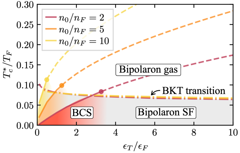
Figure 3: Critical pairing temperatures $T_{c}^{*}/T_{F}$ as a function of trion energy $\epsilon_{T}/\epsilon_{F}$ for various condensate densities. In the BCS limit where $T_{c}^{*}$ is close to the BKT temperature $T_{c}$ (see Fig. 4) the data is shown as solid lines, while at strong coupling bipolarons are formed and the dashed lines represent their dissociation temperature. The dash-dotted lines give $T_{c}=T_{BKT}$ where the bipolaron gas turns superfluid.

As $\epsilon_{T}/\epsilon_{F}$ is increased, $T_{c}^{*}/T_{F}$ increases monotonously. Similarly, $T_{c}^{*}$ increases with $n_{0}$, reflecting the role of excitons as the mediators of interactions. Increasing interactions and condensate density leads to dressing of bosons and fermions by many-body fluctuations. This results in a strong increase of the boson and fermion chemical potentials (see [69]) as imposed by the conditions (i) and (ii). Since the chemical potentials enter the propagators in our diagrammatics, they suppress pairing fluctuations. Despite this suppression, we find that $T_{c}^{*}$ keeps on increasing without apparent bound.

In the weak-coupling limit, where $T_{c}^{*}$ is small, an effective BCS theory applies. In the BCS regime, it has been established that $T_{c}^{*}$ is close to the actual BKT transition temperature $T_{c}$ towards superfluidity [98, 65, 99]. This equivalence typically applies when the size of Cooper pairs $l_{C}$ is extended over many interfermion distances $d{\sim}k_{F}^{-1}$. However, as $l_{C}$ becomes comparable to the interfermion distance, $T_{c}^{*}$ rather starts to indicate only the formation of pairs but does not imply their transition into a superfluid state, i.e. $T_{c}<T_{c}^{*}$.

At strong coupling a different criterion to determine $T_{c}$ is thus required. At zero temperature the vertex described in Superconductivity induced by strong electron-exciton coupling in doped atomically thin semiconductor heterostructures admits a bound state between two electrons even in the polaron limit where $n_{F}=0$, $n_{0}>0$ [100], representing a bipolaron. By determining where the bipolaron energy $E_{BP}$ becomes comparable to the Fermi energy $\epsilon_{F}$, we obtain an estimate for where the Cooper pair size becomes comparable to the interparticle distance, $l_{C}\approx d$. To this end, we calculate $E_{BP}$ by solving Superconductivity induced by strong electron-exciton coupling in doped atomically thin semiconductor heterostructures in the polaron limit. The corresponding critical values of $[\epsilon_{T}/\epsilon_{F}]^{c}$ are shown in Fig. 3 as dots and the full dependence on $n_{0}/n_{F}$ is shown in Fig. 4. For interaction strengths beyond $[\epsilon_{T}/\epsilon_{F}]^{c}$ a description in terms of pairs that immediately condense as they form is clearly invalid. In this regime, $T_{c}^{*}$ should instead be regarded as the molecular dissociation temperature of bipolarons. Bipolarons at $T_{c}^{*}$ form a thermal bipolaron gas that has to be cooled further to facilitate the transition into a superfluid state.

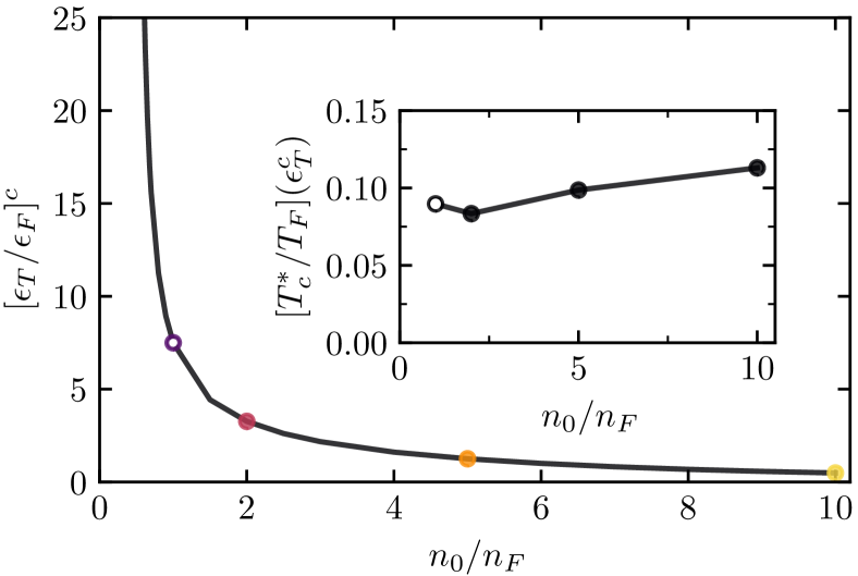
Figure 4: Critical interaction strength $\epsilon_{T}/\epsilon_{F}$ (as a function of condensate density $n_{0}/n_{F}$) beyond which the bipolaron binding energy exceeds the Fermi energy. Colored points mark densities $n_{0}/n_{F}$ shown in Fig. 3. Inset: Critical temperature at the critical interaction strengths. For illustration we also show a data point for $n_{0}/n_{F}=1$ (open circle) where trion formation might deplete the condensate to a degree beyond our description [79, 80, 31, 33, 32].

For large $\epsilon_{T}/n_{0}$, bipolarons are sufficiently deeply bound that, at finite fermion density $n_{F}>0$, the system can be described by an effective theory of weakly interacting, rigid bosons using BKT theory [101, 102, 103, 65]. To estimate the critical temperature for the BKT transition into the superfluid state, we employ the Nelson criterion [101, 102, 103, 65],

$$T_{BKT}=\frac{2\pi n_{F}}{m_{BP}}\frac{1}{\log\left(\frac{\eta}{4\pi}\log\left(\frac{1}{n_{F}d_{*}^{2}}\right)\right)}.$$ (5)

Here the density of bipolarons is given by $n_{F}$, and $\eta\approx 380$ [65]. The bipolaron-bipolaron scattering length $d_{*}$ and effective bipolaron effective mass $m_{BP}$ are computed in the SM [69]. We note that the bipolarons remain relatively light which, similar to recent studies of bipolarons in the Peierls model [104, 105], facililates rather large values of $T_{c}$. The BKT transition temperatures obtained from Eq. 5 are shown in Fig. 3 as dashed-dotted lines. We see that the predictions from the BCS limit and the bipolaron theory intersect in the expected region indicated by the dots in Fig. 3.

Connecting these two results for $T_{c}$ from weak to strong coupling makes evident that the systems is governed by an emerging BCS-BEC crossover from superfluid Cooper pairs to a quasi-condensate of bipolarons.

Remarkably, despite originating from mediated interactions, the maximal $T_{c}/T_{F}$ in our model reaches values on the order of $10\%$, not far below the values obtained in the conventional model of the BCS-BEC crossover [106, 107, 98, 108, 58, 109, 110, 111, 65, 112, 113] which describes fermions that interact via direct, short-range potentials. We estimate this maximum value of $T_{c}/T_{F}$ by considering the temperature at the endpoints calculated in Fig. 3. The results are shown in the inset of Fig. 4 and demonstrate insensitivity with respect to the density of the exciton gas. In particular at exciton densities $n_{0}/n_{F}\gg 1$ the critical temperature remains robust. At such densities, neither thermal nor interaction-driven depletion of the condensate —not taken into account in our work— plays a significant role, attesting to the robustness of the mechanism of trion-enhanced, exciton mediated superconductivity.

Conclusion.— Incorporating the strong-coupling physics of exciton-electron mixtures, we have shown that exciton-mediated pairing of electrons in doped, atomically thin semiconductor heterostructures offers a promising route towards realizing superconductivity at high temperatures $T_{c}/T_{F}$. Our work applies in the experimentally realizable regime where exciton densities are larger than the electron density. A unified description of the strong-coupling regime where all scales, $\epsilon_{F}$, $n_{0}$, $\epsilon_{T}$ are of the same order is an interesting venue for future studies. In this regime, a fully self-consistent treatment of quasiparticles is required and interaction driven condensate depletion may have a significant effect.

In our work we did not discuss the impact of the underlying repulsive Coulomb interaction. While this can be justified by screening at sufficient electron densities (as evidenced by the agreement of the model (Superconductivity induced by strong electron-exciton coupling in doped atomically thin semiconductor heterostructures) with experimental observations [91]), it remains an open problem to formally study the interplay of Coulomb screening and pairing fluctuations. Ultimatively this competition may result in $p$-wave pairing becoming the leading instability in certain density regimes [114] while, in turn, higher-order correlation functions [97] may favor the $s$-wave pairing studied in this work.

Note added.—Zerba et al. explored a complementary scheme using Feshbach resonances for inducing p-wave superconductivity in Bose-Fermi mixtures realized with TMD heterostructures [115].

Acknowledgements.— We thank Eugene Demler, Nigel Cooper and Verena Köder for inspiring discussions. This work was supported by the Deutsche Forschungsgemeinschaft under Germany’s Excellence Strategy EXC 2181/1 - 390900948 (the Heidelberg STRUCTURES Excellence Cluster). The work of A.I. was supported by the Swiss National Science Foundation (SNSF) under Grant Number 200021-204076. J.v.M. is also supported by a fellowship of the International Max Planck Research School for Quantum Science and Technology (IMPRS-QST).

Supplemental Material for ‘Superconductivity induced by strong electron-exciton coupling in doped atomically thin semiconductors’

Jonas von Milczewski, Xin Chen, Ataç İmamoğlu, and Richard Schmidt

In this supplemental material, we discuss details of the calculations and analysis that led to the results presented in the main text. Throughout this supplemental material we work in units where $m=1/2$. Note, that in principle the action in Superconductivity induced by strong electron-exciton coupling in doped atomically thin semiconductor heterostructures involves terms of the form $gn_{0}$. However, $g$ is regulated using an upper momentum cutoff $\Lambda$ [77] and thus these terms vanish as $\Lambda$ is increased and are hence left out in $G_{0}$ and Superconductivity induced by strong electron-exciton coupling in doped atomically thin semiconductor heterostructures of the main text.

I Renormalization group analysis of the extended Fröhlich model in the few-body limit

We conduct a renormalization group (RG) analysis in the few-body limit of the running coupling constants within the Hamiltonian given by Superconductivity induced by strong electron-exciton coupling in doped atomically thin semiconductor heterostructures in the main text.To begin, we consider the action

$$S =\int_{Q}\phi^{\ast}_{Q}P_{\phi}(Q)\phi_{Q}+\psi_{Q}^{\ast}P_{\psi}(Q)\psi_{Q}+\lambda\int_{Q,P}\psi^{*}_{Q}\psi^{\phantom{*}}_{P}\left(\phi^{*}_{P-Q}+\phi^{\phantom{*}}_{Q-P}\right)+g\int_{Q,P,P^{\prime}}\psi^{*}_{P}\psi^{\phantom{*}}_{Q-P}\phi^{*}_{P^{\prime}}\phi^{\phantom{*}}_{Q-P^{\prime}}.$$ (S1)

The $\lambda$ term originates from the term in Eq. (1) of the main text which is proportional to a condensate density $n_{0}$, $\lambda{\sim}\sqrt{n_{0}}g$. We will use a functional RG approach in the following [116]. The truncation of the relevant flowing effective action corresponding to Eq. S1 is given by

$$\Gamma_{k}=\int_{Q}\phi^{\ast}_{Q}P_{\phi}(Q)\phi_{Q}+\psi_{Q}^{\ast}P_{\psi}(Q)\psi_{Q}+\lambda_{k}\int_{Q,P}\psi^{*}_{Q}\psi^{\phantom{*}}_{P}\left(\phi^{*}_{P-Q}+\phi^{\phantom{*}}_{Q-P}\right)+g_{k}\int_{Q,P,P^{\prime}}\psi^{*}_{P}\psi^{\phantom{*}}_{Q-P}\phi^{*}_{P^{\prime}}\phi^{\phantom{*}}_{Q-P^{\prime}}.$$ (S2)

Here $k$ is the RG scale, above which all fluctuations have been integrated out. It runs from the UV cutoff scale $k=\Lambda$ to the infrared at $k=0$. As before, $\psi$ denotes the electron (fermion) field, while $\phi$ denotes the exciton (boson) field. We fix the initial conditions such that $\lambda_{k=\Lambda}=\lambda$ and $g_{k=\Lambda}=g$. In the following, we treat these running couplings as independent to establish a complete picture of the RG flow of the model. We disregard that the flowing coupling constants may acquire a frequency and momentum dependence during the RG flow and instead use a projection

$$\lambda_{k} =\left.\frac{\delta^{3}}{\delta\phi^{*}_{0}\delta\psi^{\phantom{*}}_{0}\delta\psi^{*}_{0}}\Gamma_{k}\right|_{\psi=\phi=0}$$ (S3)

$$g_{k} =\left.\frac{\delta^{4}}{\delta\phi^{\phantom{*}}_{0}\delta\phi^{*}_{0}\delta\psi^{\phantom{*}}_{0}\delta\psi^{*}_{0}}\Gamma_{k}\right|_{\psi=\phi=0},$$ (S4)

where the subindices on the fields indicate a projection onto zero frequency and momentum. Using the Wetterich equation [116] we compute the flow of the effective action $\Gamma_{k}$

$$\partial_{k}\Gamma_{k}=\frac{1}{2}\operatorname{STr}\Big{[}\Big{(}\Gamma_{k}^{(2)}+R_{k}\Big{)}^{-1}\partial_{k}R_{k}\Big{]},$$ (S5)

from which we can determine the flow of the coupling constants $\lambda_{k}$ and $g_{k}$.

The corresponding diagrams are shown in Fig. S1. Choosing a sharp momentum regulator as done in Refs. [75, 32], the RG flows are given by

$$\partial_{k}g_{k} =\tilde{\partial}_{k}\int_{P}\left(-\frac{g_{k}^{2}}{P_{\psi}(P)}+\frac{3\lambda_{k}^{2}g_{k}}{P_{\psi}(P)^{2}}-\frac{2\lambda_{k}^{4}}{P_{\psi}(P)^{3}}\right)\left(\frac{1}{P_{\phi}(P)}+\frac{1}{P_{\phi}(-P)}\right)\Theta(|\mathbf{p}|-k)$$ (S6)

$$\partial_{k}\lambda_{k} =\tilde{\partial}_{k}\int_{P}\left(-\frac{g_{k}\lambda_{k}}{P_{\psi}(P)}+\frac{\lambda_{k}^{3}}{P_{\psi}(P)^{2}}\right)\left(\frac{1}{P_{\phi}(P)}+\frac{1}{P_{\phi}(-P)}\right)\Theta(|\mathbf{p}|-k).$$ (S7)

$$\partial_{k}g_{k}=\ \tilde{\partial}_{k} \left[\leavevmode\hbox to0pt{\vbox to0pt{\text{[drawing]}}}+\leavevmode\hbox to0pt{\vbox to0pt{\text{[drawing]}}}+2\leavevmode\hbox to0pt{\vbox to0pt{\text{[drawing]}}}+2\leavevmode\hbox to0pt{\vbox to0pt{\text{[drawing]}}}\right.$$

$$+2\left.\leavevmode\hbox to0pt{\vbox to0pt{\text{[drawing]}}}+2\leavevmode\hbox to0pt{\vbox to0pt{\text{[drawing]}}}+\leavevmode\hbox to0pt{\vbox to0pt{\text{[drawing]}}}+\leavevmode\hbox to0pt{\vbox to0pt{\text{[drawing]}}}\right]$$

$$\partial_{k}\lambda_{k}=\ \tilde{\partial}_{k} \left[\leavevmode\hbox to0pt{\vbox to0pt{\text{[drawing]}}}+\leavevmode\hbox to0pt{\vbox to0pt{\text{[drawing]}}}+\leavevmode\hbox to0pt{\vbox to0pt{\text{[drawing]}}}+\leavevmode\hbox to0pt{\vbox to0pt{\text{[drawing]}}}\right]$$

Figure S1: Diagrammatic representation of the flow equations of the coupling constants $g_{k}$ and $\lambda_{k}$. In the flows of $\partial_{k}g_{k}$ (Eq. S6) and $\partial_{k}\lambda_{k}$ (Eq. S7) dashed lines denote exciton propagators and solid lines denote electron propagators. Dots denote the electron-exciton three point vertex ${\sim}\lambda_{k}$, while squares denote the electron-exciton four point vertex ${\sim}g_{k}$.

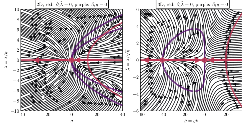
Figure S2: Flow chart for the dimensionless coupling constants $\tilde{\lambda}$ and $\tilde{g}$ in (a) two dimensions and (b) three dimensions, obtained from a functional renormalization group analysis of the model Eq. S2. Using the dimensionless RG scale $t=\log(k/\Lambda)$, for given values of $g_{k}$ and $\tilde{\lambda}_{k}=\lambda_{k}/k$ ( $\tilde{g}_{k}=g_{k}k$ and $\tilde{\lambda}_{k}=\lambda_{k}/\sqrt{k}$ in 3D) the direction of the RG flow, given by the beta functions $\partial_{t}\tilde{\lambda}_{t}$ and $\partial_{t}g_{t}$ ($\partial_{t}\tilde{\lambda}_{t},\partial_{t}\tilde{g}_{t}$ in 3D) is shown. In the left panel the purple curves denote points with $\tilde{\lambda}_{t}^{2}=g_{t}$ and $\tilde{\lambda}_{t}^{2}=2g_{t}$ where $\partial_{t}g_{t}=0$ while the red curves denote points with $g_{t}=(8\pi+\tilde{\lambda}_{t}^{2})/2$ and $\tilde{\lambda}_{t}=0$ where $\partial_{t}g=0$. Similarly, in the right panel the purple curve denotes points with $\partial_{t}\tilde{g}_{t}=0$ and the red curves represent points with $\partial_{t}\tilde{\lambda}_{t}=0$. RG fixed points occur when the red and purple lines cross. The thick arrows indicate the flow of $g$ and $\tilde{g}$ when $\tilde{\lambda}=0$.

I.1 Flow of coupling constants in two dimensions

To evaluate the flow equations in the few-body limit, we set the chemical potentials to $\mu_{B}=\mu_{F}=0$ following similar RG analysis, e.g., of the BEC-BCS crossover [71]. After performing the momentum and frequency integrals, defining a dimensionless RG scale

$$t=\log\left(\frac{k}{\Lambda}\right)$$ (S8)

and the dimensionless coupling constant

$$\tilde{\lambda}_{k}=\frac{\lambda_{k}}{k},$$ (S9)

the flow equations in dimensionless form read

$$\partial_{t}g_{t} =\frac{1}{2\pi}\left(\frac{g_{t}^{2}}{2}-\frac{3}{4}\tilde{\lambda}_{t}^{2}g_{t}+\frac{\tilde{\lambda}_{t}^{4}}{4}\right)$$ (S10)

$$\partial_{t}\tilde{\lambda}_{t} =\frac{1}{2\pi}\left(\frac{\tilde{\lambda}_{t}g_{t}}{2}-\frac{\tilde{\lambda}_{t}^{3}}{4}\right)-\tilde{\lambda}_{t}.$$ (S11)

The corresponding flow chart is shown in Fig. S2, where flows begin in the UV at $t=0$ and end in the IR at $t=-\infty$. For a given point in the flow diagram the arrows point in the direction of the flow. As one can see for $\tilde{\lambda}_{k=\Lambda}=0$ and $g_{k=\Lambda}>0$ the coupling constant $g$ flows towards the Gaussian, i.e. weak-coupling, fixed point, $\lim_{k\to 0}g_{k}=0$. On the other hand, for $\tilde{\lambda}_{k=\Lambda}=0$ and $g_{k=\Lambda}<0$ the coupling flows to $\lim_{k\to 0}g_{k}=-\infty$, indicating bound state formation; this RG behavior reflects that a bound state exists for any attractive interaction in 2D [57]. For $\tilde{\lambda}_{k=\Lambda}=\pm\sqrt{8\pi}$, $g_{k=\Lambda}=\pm 8\pi$ we find two additional repulsive fixed points, while for all other initial values with $|\tilde{\lambda}_{k=\Lambda}|>0$ the flows are always driven towards $\lim_{k\to 0}g_{k}=-\infty$, meaning that bound state formation is inevitable and $g_{k}$ always represents a relevant correlation function that cannot be ignored.

I.2 Flow of coupling constants in three dimensions

For completeness we also perform the RG analysis in three dimensions. After again using $t=\log(k/\Lambda)$ we can define the dimensionless coupling constants

$$\tilde{g}_{k}=g_{k}k,$$ (S12)

$$\tilde{\lambda}_{k}=\frac{\lambda_{k}}{\sqrt{k}}$$ (S13)

and obtain the flow equations

$$\partial_{t}\tilde{g}_{t} =\frac{1}{2\pi^{2}}\left(\frac{\tilde{g}_{t}^{2}}{2}-\frac{3}{4}\tilde{\lambda}_{t}^{2}\tilde{g}^{\phantom{2}}_{t}+\frac{\tilde{\lambda}_{t}^{4}}{4}\right)+\tilde{g}_{t}$$ (S14)

$$\partial_{t}\tilde{\lambda}_{t} =\frac{1}{2\pi^{2}}\left(\frac{\tilde{\lambda}_{t}\tilde{g}_{t}}{2}-\frac{\tilde{\lambda}_{t}^{3}}{4}\right)-\frac{\tilde{\lambda}_{t}}{2}.$$ (S15)

The resulting flow chart is shown in Fig. S2(b). For $\tilde{\lambda}_{k=\Lambda}=0$ it shows three different qualitative regions

$$\lim_{k\to 0}\tilde{g}_{k}=\left\{\begin{aligned} &0^{+},&&\text{for }\tilde{g}_{k=\Lambda}>0\\ &0^{-},&&\text{for }-4\pi^{2}<\tilde{g}_{k=\Lambda}<0\\ &-\infty,&&\text{for }\tilde{g}_{k=\Lambda}<-4\pi^{2}.\end{aligned}\right.$$ (S16)

which yield different results with respect to the relevance of $\tilde{g}_{k}$. For $\tilde{\lambda}_{k=\Lambda}\neq 0$, on the other hand, both dimensionless coupling constants are always relevant:

$$\lim_{k\to 0}\tilde{g}_{k}=-\infty$$ (S17)

$$\lim_{k\to 0}\tilde{\lambda}_{k}=\text{sign}(\tilde{\lambda}_{k=\Lambda})\infty$$ (S18)

again demonstrating that there exists no scenario where bound state formation becomes irrelevant. Note, the fixed point at $\tilde{g}=-1$, $\tilde{\lambda}=0$ is the well-known fixed point representing the regime of unitary interactions in the BEC-BCS crossover in three dimensions.

I.3 Discussion

The flows of coupling constants in Fig. S2 show a qualitatively similar picture in both two and three dimensions. Without the electron-exciton three-point vertex ${\sim}\lambda_{k}$ the relevance of the four-point vertex $g_{k}$ is dependent on the initial value of the four point vertex $g$. In both cases, for repulsive initial values $g>0$ the four point vertex is irrelevant and vanishes as a result of the renormalization process $\lim_{k\to 0}g_{k}=0$. For attractive initial values $g<0$ in two dimensions the coupling is relevant and flows to strong-coupling physics featuring an exciton-electron bound state. In three dimensions, it is not sufficient that the coupling is attractive, but rather it needs to be sufficiently attractive $g<-4\pi^{2}/\Lambda$. If these conditions are fulfilled, the few-body system flows to strong coupling and thus the bound state physics needs to be taken into account.

Considering the electron-exciton three-point vertex ${\sim}\lambda_{k}$, the qualitative nature of the relevance of the coupling changes. In two and three dimensions, apart from the two repulsive fixed points in 2D, a finite value of $\lambda$ always leads to the system flowing to strong coupling, highlighting the relevance of the four-body vertex. This behaviour is akin to the in medium behaviour of the two-body bound state in three dimensions: as the three-point vertex may be regarded as stemming from the immersion of a two-body problem within a bosonic medium $\lambda{\sim}\sqrt{n_{0}}g$, represented by the condensate. While in the vacuum two-body limit in three dimensions the bound state exists only for positive scattering lengths, when introducing a bosonic or fermionic medium, however, the two-body bound state exists for all scattering lengths.

This analysis thus indicates that the four-point vertex is relevant and therefore needs to be taken into consideration, including the associated strong-coupling physics.

II Trion self-energy

The trion self-energy $\Sigma_{t}^{\sigma}$ (see Fig. 2(d)) is given by

$$\frac{\Sigma^{\sigma}_{t}(\mathbf{p},\omega)}{h^{2}} =\lim_{T\to 0}\int_{\mathbf{q},n}G^{0}_{\psi^{*}_{\sigma}\psi^{\phantom{*}}_{\sigma}}(\mathbf{p}-\mathbf{q},\omega-\nu_{n})G^{0}_{\phi^{*}\phi^{\phantom{*}}}(\mathbf{q},\nu_{n})$$

$$=\frac{1}{(2\pi)^{3}}\int d\mathbf{q}d\nu\frac{1}{P_{\psi}(\mathbf{p}-\mathbf{q},\omega-\nu)P_{\phi}(\mathbf{q},\nu)}.$$ (S19)

Here we have approximated the diagram by its zero temperature $T=0$ expression which allows us to obtain an analytical result that can be readily employed in the following numerical computation. Based on favorable comparisons of $T=0$ theory and experimental observations at finite temperature in the Fermi polaron limit, we expect finite temperature corrections to yield only small quantitative changes to the results. The microscopic short-range interaction has to be regularized and renormalized which gives the condition [77, 79, 32]

$$P_{t}^{0}(\mathbf{q},\omega)=\frac{h^{2}}{(2\pi)^{2}}\int_{|\mathbf{q}|>\Lambda}d\mathbf{q}\frac{1}{\epsilon_{T}+2\mathbf{q}^{2}},$$ (S20)

where $\Lambda$ is the upper momentum cutoff [77], so that

$$P_{t}(\mathbf{q},\omega)=P_{t}^{0}(\mathbf{q},\omega)-\Sigma^{\sigma}_{t}(\mathbf{p},\omega).$$ (S21)

This function is related to the non-self-consistent $T$-matrix used commonly in single-channel approaches via $T(\mathbf{p},\omega)=-h^{2}/P_{t}(\mathbf{q},\omega)$ [32]. For $\mu_{F}>0$ it is given in Eq. (3) of Ref [78]. For $\mu_{F}<0$ and $\omega>0$ it is given by [32]

$$P_{t}(\mathbf{p},\omega)=-h^{2}\frac{i\pi+\log\left(\frac{\epsilon_{T}}{\mu_{F}+\mu_{B}-\mathbf{p}^{2}/2+i\omega}\right)}{8\pi},\ (-\mu_{F},\omega>0)$$ (S22)

and one can use $P_{t}(\mathbf{p},\omega)=P_{t}(\mathbf{p},-\omega)^{*}$ for $\omega<0$.

III Renormalized Green’s functions

Having introduced the trion self-energy to capture the strong coupling physics and the trion formation between electrons and excitons, the propagators used in the remaining diagrams are computed using Eq. 3 of the main text. They are thus obtained as

$$G_{\psi^{*}_{\sigma}\psi^{\phantom{*}}_{\sigma}}(\mathbf{p},\omega) =\left(\frac{P_{t}}{P_{t}P_{\psi}-h^{2}n_{0}}\right)(\mathbf{p},\omega)$$ (S23)

$$G_{t^{*}_{\sigma}t^{\phantom{*}}_{\sigma}}(\mathbf{p},\omega) =\left(\frac{P_{\psi}}{P_{t}P_{\psi}-h^{2}n_{0}}\right)(\mathbf{p},\omega)$$ (S24)

$$G_{t^{*}_{\sigma}\psi^{\phantom{*}}_{\sigma}}(\mathbf{p},\omega) =\left(\frac{-h\sqrt{n_{0}}}{P_{t}P_{\psi}-h^{2}n_{0}}\right)(\mathbf{p},\omega)$$ (S25)

$$G_{\psi^{*}_{\sigma}t^{\phantom{*}}_{\sigma}}(\mathbf{p},\omega) =\left(\frac{-h\sqrt{n_{0}}}{P_{t}P_{\psi}-h^{2}n_{0}}\right)(\mathbf{p},\omega),$$ (S26)

and $G_{\phi^{*}\phi^{\phantom{*}}}=1/P_{\phi}(\mathbf{p},\omega)$, where changing the order of fermionic (bosonic) indices results in an additional factor of $-1$ (1). The remaining matrix elements of the matrix values Green’s function $G$ vanish.

IV Exciton self-energy

As discussed in the main text, the bosonic chemical potential is fixed by the Hugenholtz-Pines relation used in the condition (ii) of the main text. The exciton self-energy entering this condition is represented by the diagram in Fig. 2(f). It is given by

$$\Sigma_{B}(\mathbf{q},\nu_{m})=\frac{h^{2}T}{(2\pi)^{2}}\int d\mathbf{p}\sum_{n,\sigma} G_{t^{*}_{\sigma}t^{\phantom{*}}_{\sigma}}(\mathbf{p}+\mathbf{q},\omega_{n}+\nu_{m})G_{\psi^{\phantom{*}}_{\sigma}\psi^{*}_{\sigma}}(\mathbf{p},\omega_{n}).$$ (S27)

Instead of numerically evaluating the Matsubara sum directly (leading to poor convergence), we rather compute an equivalent contour integral for which a contour is laid around the Matsubara frequencies and then deformed to the real axis to arrive at

$$\Sigma_{B}(0,0) =\sum_{\sigma}\frac{1}{4\pi^{3}}\int d\mathbf{p}\int_{-\infty}^{\infty}d\Omega n_{F}(\Omega)\Im\left(\frac{P_{t}(\mathbf{p},-iz)P_{\psi}(\mathbf{p},-iz)}{\left[P_{t}(\mathbf{p},-iz)P_{\psi}(\mathbf{p},-iz)-h^{2}n_{0}\right]^{2}}\right)\Bigg{|}_{z=\Omega+i\epsilon}$$ (S28)

where $n_{F}(\Omega)=1/(1+e^{\Omega/T})$ is the Fermi-distribution function. This allows for efficient numerical evaluation.

V Fermion number equation

Similar to the exciton self-energy $\Sigma_{B}$, the Matsubara summation for the number equation, entering the condition (i) of the main text, converges only slowly. Hence we again deform the integration contour to wrap around the real axis. In this way, the fermion density can be computed as follows:

$$n_{F}= -\frac{1}{(2\pi)^{2}}\int d\mathbf{p}\frac{1}{\beta}\sum_{n}\frac{P_{t}(\mathbf{p},\omega_{n})}{P_{t}(\mathbf{p},\omega_{n})P_{\psi}(\mathbf{p},\omega_{n})-h^{2}n_{0}}$$

$$= \frac{1}{(2\pi)^{2}}\int d\mathbf{p}\frac{1}{\pi}\int_{-\infty}^{\infty}d\Omega n_{F}(\Omega)\Im\left(\frac{P_{t}(\mathbf{p},-iz)}{P_{t}(\mathbf{p},-iz)P_{\psi}(\mathbf{p},-iz)-h^{2}n_{0}}\right)\Bigg{|}_{z=\Omega+i\epsilon}$$ (S29)

VI Computation of electron-trion scattering vertex

We perform an $s$-wave projection of the electron-trion scattering vertex in which we consider scattering at the Fermi-wavevector $k_{F}$ of the balanced two component Fermi gas of electrons

$$\tilde{\gamma}_{\sigma,\sigma^{\prime}}=\frac{1}{2\pi}\int d\theta_{\mathbf{k},\mathbf{k}^{\prime}}\frac{1}{2}\Big{[} \gamma(K_{+}-K_{+}^{\prime},K_{+},K_{+}^{\prime})_{\sigma,\sigma^{\prime}}+\gamma(K_{-}-K_{-}^{\prime},K_{-},K_{-}^{\prime})_{\sigma,\sigma^{\prime}}\Big{]}.$$ (S30)

Here $K_{\pm}=(\mathbf{k},\pm\pi T),K_{\pm}^{\prime}=(\mathbf{k}^{\prime},\pm\pi T)$, $|\mathbf{k}|=|\mathbf{k}^{\prime}|=k_{F}$, $\theta_{\mathbf{k},\mathbf{k}^{\prime}}$ denotes the angle between $\mathbf{k}$ and $\mathbf{k}^{\prime}$ and $\tilde{\gamma}_{\sigma,\sigma^{\prime}}$ is used within Superconductivity induced by strong electron-exciton coupling in doped atomically thin semiconductor heterostructures.

Using Superconductivity induced by strong electron-exciton coupling in doped atomically thin semiconductor heterostructures and S30 the expression for the $s$-wave projection of the electron-electron scattering vertex is then given by

$$\tilde{\gamma}_{\sigma,\sigma^{\prime}}=\tilde{\gamma}^{0}_{\sigma,\sigma^{\prime}}+\tilde{\gamma}_{\sigma,\sigma^{\prime}}\int_{\mathbf{p}} \frac{T}{2}\sum_{\omega_{n}}\left(\frac{1}{P_{\phi}(\mathbf{p}-\mathbf{k},\omega_{n}+\pi T)}+\frac{1}{P_{\phi}(\mathbf{p}-\mathbf{k},\omega_{n}-\pi T)}\right)$$

$$\quad\times\frac{h^{2}n_{0}}{\left[P_{t}(\mathbf{p},\omega_{n})P_{\psi}(\mathbf{p},\omega_{n})-h^{2}n_{0}\right]\left[P_{t}(-\mathbf{p},-\omega_{n})P_{\psi}(-\mathbf{p},-\omega_{n})-h^{2}n_{0}\right]},$$ (S31)

where $|\mathbf{k}|=k_{F}$. The pairing instability is computed by rearranging Eq. S31 to $\tilde{\gamma}_{\sigma,\sigma^{\prime}}=\tilde{\gamma}^{0}_{\sigma,\sigma^{\prime}}/(1-F)$ and solving for $F=1$ where

$$F=\frac{\tilde{\gamma}_{\sigma,\sigma^{\prime}}-\tilde{\gamma}^{0}_{\sigma,\sigma^{\prime}}}{\tilde{\gamma}_{\sigma,\sigma^{\prime}}}.$$ (S32)

$F$ represents the integral and sum part in Eq. S31. As this integral decays faster in frequency than the number equation and the exciton self-energy, the Matsubara summation in Eq. S31 can be directly computed numerically, without the need to deform the integration contour.

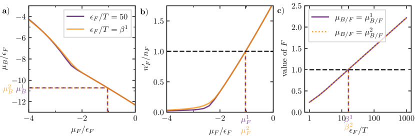
Figure S3: Exemplary optimization procedure to simultaneously solve for the Hugenholtz-Pines relation and the number equation at $\epsilon_{T}=5\epsilon_{F}$, $n_{0}/n_{F}=1$. (a) The boson chemical potential $\mu_{B}(\mu_{F},n_{0},\epsilon_{T},T)$ to fulfill the Hugenholtz-Pines relation is shown as a function of the fermion chemical potential. At an initial temperature of $T_{0}=\epsilon_{F}/50$ (purple) the critical boson chemical potential is computed as a function of the fermion chemical potential and the resulting pairs of ($\mu_{F},\mu_{B}(\mu_{F},n_{0},\epsilon_{T},T_{0})$) are used to compute the corresponding fermion density $n^{\prime}_{F}(\mu_{F},\mu_{B}(\mu_{F},n_{0},\epsilon_{T},T_{0}))$, shown in (b). The point at which $n^{\prime}_{F}(\mu^{1}_{F},\mu_{B}(\mu^{1}_{F},n_{0},\epsilon_{T},T_{0}))=n_{F}$ is used to determine $\mu_{F}^{1}$. From this, the corresponding boson chemical potential $\mu_{B}^{1}$ is computed as $\mu_{B}^{1}=\mu_{B}(\mu^{1}_{F},n_{0},\epsilon_{T},T_{0})$. In (c) the value of F obtained using $\mu_{F}^{1}$ and $\mu_{B}^{1}$ is shown for varying temperatures and it is used to determine a critical inverse temperature $\beta^{1}=1/T_{1}$ by locating where $F=1$. This temperature is used in a second iteration (yellow) from which $\mu_{F}^{2}$ and $\mu_{B}^{2}$ are found which are used in (c) to find a critical inverse temperature $\beta^{2}=1/T_{2}$. This cycle is repeated until the chemical potentials and critical temperatures are found to be converged.

VII Determining the critical pairing temperature

To estimate the critical pairing temperature for given values of $\epsilon_{T}/\epsilon_{F}$ and $n_{0}/n_{F}$, the critical pairing condition needs to be solved for, while fulfilling the number equation (i) and the Hugenholtz-Pines relation (ii). This is done in a self-consistent optimization procedure which we describe in the following.

First, for given values of $n_{0}/\epsilon_{F},\epsilon_{T}/\epsilon_{F}$ and an initial temperature of $T_{0}=\epsilon_{F}/50$ the critical boson chemical potential to fulfill the Hugenholtz-Pines relation (i) is computed as $\mu_{B}(\mu_{F},n_{0},\epsilon_{T},T_{0})$ for a varying fermion chemical potential $\mu_{F}$. Next, these chemical potentials are used within the number equation Eq. S29 to compute the Fermi density $n^{\prime}_{F}(\mu_{F},\mu_{B}(\mu_{F},n_{0},\epsilon_{T},T_{0}))$. From this, the fermion chemical potential $\mu_{F}^{1}$ fulfilling $n_{F}=n^{\prime}_{F}(\mu_{F}^{1},\mu_{B}(\mu_{F}^{1},n_{0},\epsilon_{T},T_{0}))$ is found and the corresponding boson chemical potential is determined as $\mu_{B}^{1}=\mu_{B}(\mu_{F}^{1},n_{0},\epsilon_{T},T_{0})$.

Using $\mu_{F}^{1}$ and $\mu_{B}^{1}$, the critical temperature $T_{1}$ where $F=1$ is then found using Eq. S31. This critical temperature $T_{1}$ is then used as an input to find $\mu_{F}^{2}$ and $\mu_{B}^{2}$ which are in turn used to find a critical temperature $T_{2}$. This cycle is repeated until the chemical potentials and the temperature have converged to a fixed point which simultaneously satisfies the number equation, the Hugenholtz-Pines relation and the critical pairing condition. For given values of $n_{0}/\epsilon_{F},\epsilon_{T}/\epsilon_{F}$ the temperature found gives the critical pairing temperature $T_{c}^{*}$. This procedure is shown in Fig. S3 for the first two iterations of this cycle.

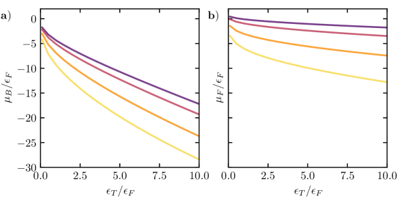
Figure S4: The boson (a) and fermion (b) chemical potentials $\mu_{B}$ and $\mu_{F}$ at the critical temperature $T_{c}^{*}$ are shown as a function of $\epsilon_{T}/\epsilon_{F}$ for the condensate densities $n_{0}/n_{F}=1$ (purple), $2$ (red), $5$ (orange), and $10$ (yellow). These potentials are simultaneous solutions of the Hugenholtz-Pines relation (i) and the number equation (ii), and to satisfy these, the chemical potentials increase in magnitude with increasing binding energy.

The resulting chemical potentials for the results shown in Fig. 3 are given in Fig. S4.

VIII Determining the bipolaron binding energy and the boundary of the BCS regime

As discussed in the main text, the method used to obtain the critical pairing temperature provides a reasonable approximation for the critical temperature of superfluidity in the regime where a BCS-type theory is appropriate. The $s$-wave projected pairing vertex $\tilde{\gamma}_{\sigma,\sigma^{\prime}}$ defined in Eq. S30 admits a bound state at $T=0$ even in the limit where the Fermi density vanishes, which we refer to as the polaron limit. Thus finding a singularity in $\tilde{\gamma}$ implies the formation of a bound state between two Bose polarons, a bound state which we refer to as the bipolaron [100]. In the strong coupling limit, we expect the superfluid transition temperature $T_{c}$ to be more accurately captured by a BKT theory of a Bose gas of bipolarons. As a result we approximate the point where the system crosses over from a BCS-type to a BKT/BEC-type behaviour as the point where the bipolaron binding energy becomes comparable to the Fermi energy and, as a result, the binding length of the bipolaron is comparable to the average fermion interparticle distance.

At $T=0$ in the polaron limit ($n_{F}=0$) the exciton self-energy vanishes identically and as a result we set $\mu_{B}=0$. Thus for given values of $\epsilon_{T}$, $n_{0}$ there exists a critical chemical potential $\mu_{F,n_{F}=0}(n_{0},\epsilon_{T})$ for which $n_{F}=0$ for $\mu_{F}<\mu_{F,n_{F}=0}(n_{0},\epsilon_{T})$ and $n_{F}>0$ for $\mu_{F}>\mu_{F,n_{F}=0}(n_{0},\epsilon_{T})$. This chemical potential in fact determines the Bose polaron energy which, for three dimensional systems, has been shown to agree remarkable well with experimental observations [66].

The binding energy of the bipolaron is determined from the divergence of $\tilde{\gamma}_{BP}$,

$$\tilde{\gamma}_{BP} =\tilde{\gamma}^{0}_{BP}+\tilde{\gamma}_{BP}\int_{\mathbf{p}}\int\frac{d\omega}{2\pi}\frac{h^{2}n_{0}}{P_{\phi}(\mathbf{p},\omega)}\frac{1}{P_{t}(\mathbf{p},\omega)P_{\psi}(\mathbf{p},\omega)-h^{2}n_{0}}\frac{1}{P_{t}(-\mathbf{p},-\omega)P_{\psi}(-\mathbf{p},-\omega)-h^{2}n_{0}},$$ (S33)

which is obtained from Eq. S31 in the limit $k_{F}\to 0$, $T\to 0$. The divergence of $\tilde{\gamma}_{BP}$ occurs at a fermion chemical potential $\mu_{F,BP}(n_{0},\epsilon_{T})<\mu_{F,n_{F}=0}(n_{0},\epsilon_{T})$. Thus the bipolaron binding energy is given as

$$E_{BP}=2\left(\mu_{F,BP}(n_{0},\epsilon_{T})-\mu_{F,n_{F}=0}(n_{0},\epsilon_{T})\right).$$ (S34)

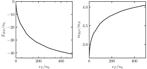
Figure S5: Bipolaron binding energy $E_{BP}$ (left) and bipolaron effective mass $m_{BP}$ (right) as a function of the trion energy $\epsilon_{T}$. The energies are given in units of condensate density $n_{0}$ while the mass is given in units of the fermion mass $m_{F}$. With increasing $\epsilon_{T}$ the bipolaron becomes deeper bound and acquires a moderate effective mass.

The resulting bipolaron binding energies are shown in Fig. S5. Hence, requiring the binding energy per particle of the bipolaron to be smaller than the Fermi energy each fermion experiences, we require $\mu_{F,n_{F}=0}(n_{0},\epsilon_{T})-\epsilon_{F}<\mu_{F,BP}(n_{0},\epsilon_{T})<\mu_{F,n_{F}=0}(n_{0},\epsilon_{T})$ for the BCS theory to be applicable. The resulting critical dimensionless interaction strengths $\epsilon_{T}/\epsilon_{F}$ for given values of $n_{0}/n_{F}$ are shown in Fig. 4 of the main text and the end points of the BCS regime are indicated in Fig. 3 of the main text.

IX Approximation of the BKT transition temperature

To approximate the critical temperature for the transition into a BKT superfluid, we use [101, 102, 103, 65]

$$T_{BKT}=\frac{2\pi n_{F}}{m_{BP}}\frac{1}{\log\left(\frac{\eta}{4\pi}\log\left(\frac{1}{n_{F}d_{*}^{2}}\right)\right)},$$ (S35)

where the density of bipolarons is given by $n_{F}$ (all fermions can be assumed to be paired into bipolarons), and $\eta\approx 380$ [65]. The bipolaron-bipolaron scattering length is given by $d_{*}$ , and $m_{BP}$ is the effective bipolaron mass. The bipolaron scattering length is approximated by the binding length of the bipolaron [65], which in turn is parametrized by the bipolaron binding energy as

$$d_{*}=\sqrt{-\frac{1}{2E_{BP}}\left(\frac{1}{m_{F}}+\frac{1}{m_{F}+m_{B}}\right)}.$$ (S36)

The bipolaron effective mass is computed by evaluating Eq. S33 at a finite incoming momentum $\mathbf{q}$ which is distributed along the two fermionic propagator legs as $\mathbf{p}+\mathbf{q}/2$ and $\mathbf{q}/2-\mathbf{p}$. From this, the bipolaron dispersion relation is computed as a function of $|\mathbf{q}|$ and the effective bipolaron mass $m_{BP}$ is obtained from a quadratic fit to this dispersion relation. The resulting bipolaron effective mass is shown in Fig. S5. The BKT transition temperatures obtained from Eq. 5 are shown in Fig. 3 of the main text.

References

- Regan et al. [2020] E. C. Regan, D. Wang, C. Jin, M. I. B. Utama, B. Gao, X. Wei, S. Zhao, W. Zhao, Z. Zhang, K. Yumigeta, M. Blei, J. D. Carlström, K. Watanabe, T. Taniguchi, S. Tongay, M. Crommie, A. Zettl, and F. Wang, Mott and generalized wigner crystal states in WSe2/WS2 moiré superlattices, Nature 579, 359 (2020).
- Shimazaki et al. [2021] Y. Shimazaki, C. Kuhlenkamp, I. Schwartz, T. Smoleński, K. Watanabe, T. Taniguchi, M. Kroner, R. Schmidt, M. Knap, and A. Imamoğlu, Optical signatures of periodic charge distribution in a mott-like correlated insulator state, Phys. Rev. X 11, 021027 (2021).
- Zhou et al. [2021] Y. Zhou, J. Sung, E. Brutschea, I. Esterlis, Y. Wang, G. Scuri, R. J. Gelly, H. Heo, T. Taniguchi, K. Watanabe, G. Zaránd, M. D. Lukin, P. Kim, E. Demler, and H. Park, Bilayer wigner crystals in a transition metal dichalcogenide heterostructure, Nature 595, 48 (2021).
- Smoleński et al. [2021] T. Smoleński, P. E. Dolgirev, C. Kuhlenkamp, A. Popert, Y. Shimazaki, P. Back, X. Lu, M. Kroner, K. Watanabe, T. Taniguchi, I. Esterlis, E. Demler, and A. Imamoğlu, Signatures of wigner crystal of electrons in a monolayer semiconductor, Nature 595, 53 (2021).
- Serlin et al. [2020] M. Serlin, C. L. Tschirhart, H. Polshyn, Y. Zhang, J. Zhu, K. Watanabe, T. Taniguchi, L. Balents, and A. F. Young, Intrinsic quantized anomalous hall effect in a moiré heterostructure, Science 367, 900 (2020).
- Xie et al. [2022] Y.-M. Xie, C.-P. Zhang, J.-X. Hu, K. F. Mak, and K. T. Law, Valley-polarized quantum anomalous hall state in moiré heterobilayers, Phys. Rev. Lett. 128, 026402 (2022).
- Cai et al. [2023] J. Cai, E. Anderson, C. Wang, X. Zhang, X. Liu, W. Holtzmann, Y. Zhang, F. Fan, T. Taniguchi, K. Watanabe, Y. Ran, T. Cao, L. Fu, D. Xiao, W. Yao, and X. Xu, Signatures of fractional quantum anomalous hall states in twisted MoTe2, Nature (2023).
- Popert et al. [2022] A. Popert, Y. Shimazaki, M. Kroner, K. Watanabe, T. Taniguchi, A. Imamoğlu, and T. Smoleński, Optical sensing of fractional quantum hall effect in graphene, Nano Lett. 22, 7363 (2022).
- Cao et al. [2018a] Y. Cao, V. Fatemi, A. Demir, S. Fang, S. L. Tomarken, J. Y. Luo, J. D. Sanchez-Yamagishi, K. Watanabe, T. Taniguchi, E. Kaxiras, R. C. Ashoori, and P. Jarillo-Herrero, Correlated insulator behaviour at half-filling in magic-angle graphene superlattices, Nature 556, 80 (2018a).
- Sharpe et al. [2019] A. L. Sharpe, E. J. Fox, A. W. Barnard, J. Finney, K. Watanabe, T. Taniguchi, M. A. Kastner, and D. Goldhaber-Gordon, Emergent ferromagnetism near three-quarters filling in twisted bilayer graphene, Science 365, 605 (2019).
- Liu et al. [2020] X. Liu, Z. Hao, E. Khalaf, J. Y. Lee, Y. Ronen, H. Yoo, D. H. Najafabadi, K. Watanabe, T. Taniguchi, A. Vishwanath, and P. Kim, Tunable spin-polarized correlated states in twisted double bilayer graphene, Nature 583, 221 (2020).
- Xi et al. [2015] X. Xi, Z. Wang, W. Zhao, J.-H. Park, K. T. Law, H. Berger, L. Forró, J. Shan, and K. F. Mak, Ising pairing in superconducting NbSe2 atomic layers, Nat. Phys. 12, 139 (2015).
- Cao et al. [2018b] Y. Cao, V. Fatemi, S. Fang, K. Watanabe, T. Taniguchi, E. Kaxiras, and P. Jarillo-Herrero, Unconventional superconductivity in magic-angle graphene superlattices, Nature 556, 43 (2018b).
- Yankowitz et al. [2019] M. Yankowitz, S. Chen, H. Polshyn, Y. Zhang, K. Watanabe, T. Taniguchi, D. Graf, A. F. Young, and C. R. Dean, Tuning superconductivity in twisted bilayer graphene, Science 363, 1059 (2019).
- Wang et al. [2020] L. Wang, E.-M. Shih, A. Ghiotto, L. Xian, D. A. Rhodes, C. Tan, M. Claassen, D. M. Kennes, Y. Bai, B. Kim, K. Watanabe, T. Taniguchi, X. Zhu, J. Hone, A. Rubio, A. N. Pasupathy, and C. R. Dean, Correlated electronic phases in twisted bilayer transition metal dichalcogenides, Nat. Mat. 19, 861 (2020).
- Wang et al. [2018] G. Wang, A. Chernikov, M. M. Glazov, T. F. Heinz, X. Marie, T. Amand, and B. Urbaszek, Colloquium: Excitons in atomically thin transition metal dichalcogenides, Rev. Mod. Phys. 90, 021001 (2018).
- Crépel et al. [2023] V. Crépel, D. Guerci, J. Cano, J. H. Pixley, and A. Millis, Topological superconductivity in doped magnetic moiré semiconductors, Phys. Rev. Lett. 131, 056001 (2023).
- Sun et al. [2021] Z. Sun, J. Beaumariage, Q. Wan, H. Alnatah, N. Hougland, J. Chisholm, Q. Cao, K. Watanabe, T. Taniguchi, B. M. Hunt, I. V. Bondarev, and D. Snoke, Charged bosons made of fermions in bilayer structures with strong metallic screening, Nano Lett. 21, 7669 (2021).
- Slagle and Fu [2020] K. Slagle and L. Fu, Charge transfer excitations, pair density waves, and superconductivity in moiré materials, Phys. Rev. B 102, 235423 (2020).
- Crépel and Fu [2021] V. Crépel and L. Fu, New mechanism and exact theory of superconductivity from strong repulsive interaction, Science Advances 7, eabh2233 (2021).
- Crépel and Fu [2022] V. Crépel and L. Fu, Spin-triplet superconductivity from excitonic effect in doped insulators, Proceedings of the National Academy of Sciences 119, 17735119 (2022).
- Crépel et al. [2022] V. Crépel, T. Cea, L. Fu, and F. Guinea, Unconventional superconductivity due to interband polarization, Phys. Rev. B 105, 094506 (2022).
- He et al. [2023] Y. He, K. Yang, J. B. Hauck, E. J. Bergholtz, and D. M. Kennes, Superconductivity of repulsive spinless fermions with sublattice potentials, Phys. Rev. Res. 5, L012009 (2023).
- Enss and Zwerger [2009] T. Enss and W. Zwerger, Superfluidity near phase separation in bose-fermi mixtures, EPJ B 68, 383 (2009).
- Laussy et al. [2010] F. P. Laussy, A. V. Kavokin, and I. A. Shelykh, Exciton-polariton mediated superconductivity, Phys. Rev. Lett. 104, 106402 (2010).
- Cotleţ et al. [2016] O. Cotleţ, S. Zeytinoǧlu, M. Sigrist, E. Demler, and A. Imamoğlu, Superconductivity and other collective phenomena in a hybrid bose-fermi mixture formed by a polariton condensate and an electron system in two dimensions, Phys. Rev. B 93, 054510 (2016).
- Kinnunen et al. [2018] J. J. Kinnunen, Z. Wu, and G. M. Bruun, Induced -wave pairing in bose-fermi mixtures, Phys. Rev. Lett. 121, 253402 (2018).
- Julku et al. [2022] A. Julku, J. J. Kinnunen, A. Camacho-Guardian, and G. M. Bruun, Light-induced topological superconductivity in transition metal dichalcogenide monolayers, Phys. Rev. B 106, 134510 (2022).
- Bertaina et al. [2013] G. Bertaina, E. Fratini, S. Giorgini, and P. Pieri, Quantum Monte Carlo Study of a Resonant Bose-Fermi Mixture, Phys. Rev. Lett. 110, 115303 (2013).
- Ludwig et al. [2011] D. Ludwig, S. Floerchinger, S. Moroz, and C. Wetterich, Quantum phase transition in bose-fermi mixtures, Phys. Rev. A 84, 033629 (2011).
- Guidini et al. [2015] A. Guidini, G. Bertaina, D. E. Galli, and P. Pieri, Condensed phase of Bose-Fermi mixtures with a pairing interaction, Phys. Rev. A 91, 023603 (2015).
- von Milczewski et al. [2022] J. von Milczewski, F. Rose, and R. Schmidt, Functional-renormalization-group approach to strongly coupled Bose-Fermi mixtures in two dimensions, Phys. Rev. A 105, 013317 (2022).
- Duda et al. [2023] M. Duda, X.-Y. Chen, A. Schindewolf, R. Bause, J. von Milczewski, R. Schmidt, I. Bloch, and X.-Y. Luo, Transition from a polaronic condensate to a degenerate fermi gas of heteronuclear molecules, Nat. Phys. 19, 720 (2023).
- Tan et al. [2023] L. B. Tan, O. K. Diessel, A. Popert, R. Schmidt, A. Imamoglu, and M. Kroner, Bose polaron interactions in a cavity-coupled monolayer semiconductor, Phys. Rev. X 13, 031036 (2023).
- Fröhlich [1954] H. Fröhlich, Electrons in lattice fields, Advances in Physics 3, 325 (1954).
- Holstein [1959] T. Holstein, Studies of polaron motion, Annals of Physics 8, 325 (1959).
- Jochim et al. [2003] S. Jochim, M. Bartenstein, A. Altmeyer, G. Hendl, S. Riedl, C. Chin, J. H. Denschlag, and R. Grimm, Bose-einstein condensation of molecules, Science 302, 2101 (2003).
- Greiner et al. [2003] M. Greiner, C. A. Regal, and D. S. Jin, Emergence of a molecular bose–einstein condensate from a fermi gas, Nature 426, 537 (2003).
- Zwierlein et al. [2003] M. W. Zwierlein, C. A. Stan, C. H. Schunck, S. M. F. Raupach, S. Gupta, Z. Hadzibabic, and W. Ketterle, Observation of bose-einstein condensation of molecules, Phys. Rev. Lett. 91, 250401 (2003).
- Regal et al. [2004] C. A. Regal, M. Greiner, and D. S. Jin, Observation of resonance condensation of fermionic atom pairs, Phys. Rev. Lett. 92, 040403 (2004).
- Zwierlein et al. [2004] M. W. Zwierlein, C. A. Stan, C. H. Schunck, S. M. F. Raupach, A. J. Kerman, and W. Ketterle, Condensation of pairs of fermionic atoms near a feshbach resonance, Phys. Rev. Lett. 92, 120403 (2004).
- Chin et al. [2004] C. Chin, M. Bartenstein, A. Altmeyer, S. Riedl, S. Jochim, J. H. Denschlag, and R. Grimm, Observation of the pairing gap in a strongly interacting fermi gas, Science 305, 1128 (2004).
- Kinast et al. [2004] J. Kinast, S. L. Hemmer, M. E. Gehm, A. Turlapov, and J. E. Thomas, Evidence for superfluidity in a resonantly interacting fermi gas, Phys. Rev. Lett. 92, 150402 (2004).
- Bourdel et al. [2004] T. Bourdel, L. Khaykovich, J. Cubizolles, J. Zhang, F. Chevy, M. Teichmann, L. Tarruell, S. J. J. M. F. Kokkelmans, and C. Salomon, Experimental study of the bec-bcs crossover region in lithium 6, Phys. Rev. Lett. 93, 050401 (2004).
- Strecker et al. [2003] K. E. Strecker, G. B. Partridge, and R. G. Hulet, Conversion of an atomic fermi gas to a long-lived molecular bose gas, Phys. Rev. Lett. 91, 080406 (2003).
- Zwierlein et al. [2006] M. W. Zwierlein, C. H. Schunck, A. Schirotzek, and W. Ketterle, Direct observation of the superfluid phase transition in ultracold fermi gases, Nature 442, 54 (2006).
- Ku et al. [2012] M. J. H. Ku, A. T. Sommer, L. W. Cheuk, and M. W. Zwierlein, Revealing the superfluid lambda transition in the universal thermodynamics of a unitary fermi gas, Science 335, 563 (2012).
- Feld et al. [2011] M. Feld, B. Fröhlich, E. Vogt, M. Koschorreck, and M. Köhl, Observation of a pairing pseudogap in a two-dimensional fermi gas, Nature 480, 75 (2011).
- Sommer et al. [2012] A. T. Sommer, L. W. Cheuk, M. J. H. Ku, W. S. Bakr, and M. W. Zwierlein, Evolution of fermion pairing from three to two dimensions, Phys. Rev. Lett. 108, 045302 (2012).
- Ries et al. [2015] M. G. Ries, A. N. Wenz, G. Zürn, L. Bayha, I. Boettcher, D. Kedar, P. A. Murthy, M. Neidig, T. Lompe, and S. Jochim, Observation of pair condensation in the quasi-2d bec-bcs crossover, Phys. Rev. Lett. 114, 230401 (2015).
- Murthy et al. [2018] P. A. Murthy, M. Neidig, R. Klemt, L. Bayha, I. Boettcher, T. Enss, M. Holten, G. Zürn, P. M. Preiss, and S. Jochim, High-temperature pairing in a strongly interacting two-dimensional fermi gas, Science 359, 452 (2018).
- Sobirey et al. [2021] L. Sobirey, N. Luick, M. Bohlen, H. Biss, H. Moritz, and T. Lompe, Observation of superfluidity in a strongly correlated two-dimensional fermi gas, Science 372, 844 (2021).
- Holten et al. [2022] M. Holten, L. Bayha, K. Subramanian, S. Brandstetter, C. Heintze, P. Lunt, P. M. Preiss, and S. Jochim, Observation of cooper pairs in a mesoscopic two-dimensional fermi gas, Nature 606, 287 (2022).
- Amelio et al. [2023] I. Amelio, N. D. Drummond, E. Demler, R. Schmidt, and A. Imamoglu, Polaron spectroscopy of a bilayer excitonic insulator, Phys. Rev. B 107, 155303 (2023).
- Ma et al. [2021] L. Ma, P. X. Nguyen, Z. Wang, Y. Zeng, K. Watanabe, T. Taniguchi, A. H. MacDonald, K. F. Mak, and J. Shan, Strongly correlated excitonic insulator in atomic double layers, Nature 598, 585 (2021).
- Zhang et al. [2022] Z. Zhang, E. C. Regan, D. Wang, W. Zhao, S. Wang, M. Sayyad, K. Yumigeta, K. Watanabe, T. Taniguchi, S. Tongay, M. Crommie, A. Zettl, M. P. Zaletel, and F. Wang, Correlated interlayer exciton insulator in heterostructures of monolayer WSe2 and moiré WS2/WSe2, Nat. Phys. 18, 1214 (2022).
- Adhikari [1986] S. K. Adhikari, Quantum scattering in two dimensions, Am. J Phys. 54, 362 (1986).
- Randeria et al. [1989] M. Randeria, J.-M. Duan, and L.-Y. Shieh, Bound states, cooper pairing, and bose condensation in two dimensions, Phys. Rev. Lett. 62, 981 (1989).
- Raja et al. [2017] A. Raja, A. Chaves, J. Yu, G. Arefe, H. M. Hill, A. F. Rigosi, T. C. Berkelbach, P. Nagler, C. Schüller, T. Korn, C. Nuckolls, J. Hone, L. E. Brus, T. F. Heinz, D. R. Reichman, and A. Chernikov, Coulomb engineering of the bandgap and excitons in two-dimensional materials, Nat. Comm. 8, 15251 (2017).
- Steinleitner et al. [2018] P. Steinleitner, P. Merkl, A. Graf, P. Nagler, K. Watanabe, T. Taniguchi, J. Zipfel, C. Schüller, T. Korn, A. Chernikov, S. Brem, M. Selig, G. Berghäuser, E. Malic, and R. Huber, Dielectric engineering of electronic correlations in a van der waals heterostructure, Nano Lett. 18, 1402 (2018).
- Mermin and Wagner [1966] N. D. Mermin and H. Wagner, Absence of ferromagnetism or antiferromagnetism in one- or two-dimensional isotropic heisenberg models, Phys. Rev. Lett. 17, 1133 (1966).
- Hohenberg [1967] P. C. Hohenberg, Existence of long-range order in one and two dimensions, Phys. Rev. 158, 383 (1967).
- Berezinsky [1972] V. L. Berezinsky, Destruction of Long-range Order in One-dimensional and Two-dimensional Systems Possessing a Continuous Symmetry Group. II. Quantum Systems., Sov. Phys. JETP 34, 610 (1972).
- Kosterlitz and Thouless [1973] J. M. Kosterlitz and D. J. Thouless, Ordering, metastability and phase transitions in two-dimensional systems, J Phys. C 6, 1181 (1973).
- Petrov et al. [2003] D. S. Petrov, M. A. Baranov, and G. V. Shlyapnikov, Superfluid transition in quasi-two-dimensional fermi gases, Phys. Rev. A 67, 031601 (2003).
- Hu et al. [2016] M.-G. Hu, M. J. Van de Graaff, D. Kedar, J. P. Corson, E. A. Cornell, and D. S. Jin, Bose polarons in the strongly interacting regime, Phys. Rev. Lett. 117, 055301 (2016).
- Jørgensen et al. [2016] N. B. Jørgensen, L. Wacker, K. T. Skalmstang, M. M. Parish, J. Levinsen, R. S. Christensen, G. M. Bruun, and J. J. Arlt, Observation of attractive and repulsive polarons in a Bose-Einstein condensate, Phys. Rev. Lett. 117, 055302 (2016).
- Yan et al. [2020] Z. Z. Yan, Y. Ni, C. Robens, and M. W. Zwierlein, Bose polarons near quantum criticality, Science 368, 190 (2020).
- [69] See Supplementary Material.
- Lurié and Macfarlane [1964] D. Lurié and A. J. Macfarlane, Equivalence between four-fermion and yukawa coupling, and the condition for composite bosons, Phys. Rev. 136, B816 (1964).
- Nikolić and Sachdev [2007] P. Nikolić and S. Sachdev, Renormalization-group fixed points, universal phase diagram, and expansion for quantum liquids with interactions near the unitarity limit, Phys. Rev. A 75, 033608 (2007).
- Chevy [2006] F. Chevy, Universal phase diagram of a strongly interacting Fermi gas with unbalanced spin populations, Phys. Rev. A 74, 063628 (2006).
- Combescot et al. [2007] R. Combescot, A. Recati, C. Lobo, and F. Chevy, Normal state of highly polarized fermi gases: Simple many-body approaches, Phys. Rev. Lett. 98, 180402 (2007).
- Punk et al. [2009] M. Punk, P. T. Dumitrescu, and W. Zwerger, Polaron-to-molecule transition in a strongly imbalanced fermi gas, Phys. Rev. A 80, 053605 (2009).
- Schmidt and Enss [2011] R. Schmidt and T. Enss, Excitation spectra and rf response near the polaron-to-molecule transition from the functional renormalization group, Phys. Rev. A 83, 063620 (2011).
- Trefzger and Castin [2012] C. Trefzger and Y. Castin, Impurity in a fermi sea on a narrow feshbach resonance: A variational study of the polaronic and dimeronic branches, Phys. Rev. A 85, 053612 (2012).
- Zöllner et al. [2011] S. Zöllner, G. M. Bruun, and C. J. Pethick, Polarons and molecules in a two-dimensional fermi gas, Phys. Rev. A 83, 021603 (2011).
- Schmidt et al. [2012] R. Schmidt, T. Enss, V. Pietilä, and E. Demler, Fermi polarons in two dimensions, Phys. Rev. A 85, 021602 (2012).
- Parish [2011] M. M. Parish, Polaron-molecule transitions in a two-dimensional fermi gas, Phys. Rev. A 83, 051603 (2011).
- Bertaina [2012] G. Bertaina, BCS-BEC crossover in two dimensions: A quantum monte carlo study, AIP Conference Proceedings 1485, 286 (2012).
- Parish and Levinsen [2013] M. M. Parish and J. Levinsen, Highly polarized fermi gases in two dimensions, Phys. Rev. A 87, 033616 (2013).
- Kroiss and Pollet [2014] P. Kroiss and L. Pollet, Diagrammatic monte carlo study of quasi-two-dimensional fermi polarons, Phys. Rev. B 90, 104510 (2014).
- Vlietinck et al. [2014] J. Vlietinck, J. Ryckebusch, and K. Van Houcke, Diagrammatic monte carlo study of the fermi polaron in two dimensions, Phys. Rev. B 89, 085119 (2014).
- Rath and Schmidt [2013] S. P. Rath and R. Schmidt, Field-theoretical study of the bose polaron, Phys. Rev. A 88, 053632 (2013).
- Isaule et al. [2021] F. Isaule, I. Morera, P. Massignan, and B. Juliá-Díaz, Renormalization-group study of bose polarons, Phys. Rev. A 104, 023317 (2021).
- Kohstall et al. [2012] C. Kohstall, M. Zaccanti, M. Jag, A. Trenkwalder, P. Massignan, G. M. Bruun, F. Schreck, and R. Grimm, Metastability and coherence of repulsive polarons in a strongly interacting fermi mixture, Nature 485, 615 (2012).
- Schirotzek et al. [2009] A. Schirotzek, C.-H. Wu, A. Sommer, and M. W. Zwierlein, Observation of fermi polarons in a tunable fermi liquid of ultracold atoms, Phys. Rev. Lett. 102, 230402 (2009).
- Koschorreck et al. [2012] M. Koschorreck, D. Pertot, E. Vogt, B. Fröhlich, M. Feld, and M. Köhl, Attractive and repulsive fermi polarons in two dimensions, Nature 485, 619 (2012).
- Ness et al. [2020] G. Ness, C. Shkedrov, Y. Florshaim, O. K. Diessel, J. von Milczewski, R. Schmidt, and Y. Sagi, Observation of a Smooth Polaron-Molecule Transition in a Degenerate Fermi Gas, Phys. Rev. X 10, 041019 (2020).
- Fritsche et al. [2021] I. Fritsche, C. Baroni, E. Dobler, E. Kirilov, B. Huang, R. Grimm, G. M. Bruun, and P. Massignan, Stability and breakdown of Fermi polarons in a strongly interacting Fermi-Bose mixture, Phys. Rev. A 103, 053314 (2021).
- Sidler et al. [2017] M. Sidler, P. Back, O. Cotlet, A. Srivastava, T. Fink, M. Kroner, E. Demler, and A. Imamoglu, Fermi polaron-polaritons in charge-tunable atomically thin semiconductors, Nat. Phys. 13, 255 (2017).
- Goldstein et al. [2020] T. Goldstein, Y.-C. Wu, S.-Y. Chen, T. Taniguchi, K. Watanabe, K. Varga, and J. Yan, Ground and excited state exciton polarons in monolayer MoSe2, J Chem. Phys. 153, 070401 (2020).
- Xiao et al. [2021] K. Xiao, T. Yan, Q. Liu, S. Yang, C. Kan, R. Duan, Z. Liu, and X. Cui, Many-body effect on optical properties of monolayer molybdenum diselenide, J Phys. Chem. Lett. 12, 2555 (2021).
- Liu et al. [2021] E. Liu, J. van Baren, Z. Lu, T. Taniguchi, K. Watanabe, D. Smirnov, Y.-C. Chang, and C. H. Lui, Exciton-polaron rydberg states in monolayer MoSe2 and WSe2, Nat. Comm. 12, 6131 (2021).
- Zipfel et al. [2022] J. Zipfel, K. Wagner, M. A. Semina, J. D. Ziegler, T. Taniguchi, K. Watanabe, M. M. Glazov, and A. Chernikov, Electron recoil effect in electrically tunable monolayers, Phys. Rev. B 105, 075311 (2022).
- Note [1] We assume equal interaction strength of -, -electrons with the excitons as the layer separation strongly suppresses exchange effects.
- Kartavtsev and Malykh [2007] O. I. Kartavtsev and A. V. Malykh, Low-energy three-body dynamics in binary quantum gases, J Phys. B 40, 1429 (2007).
- Miyake [1983] K. Miyake, Fermi Liquid Theory of Dilute Submonolayer 3He on Thin 4He II Film: Dimer Bound State and Cooper Pairs, Prog. Theor. Phys. 69, 1794 (1983).
- Maiti and Chubukov [2013] S. Maiti and A. V. Chubukov, Superconductivity from repulsive interaction, AIP Conference Proceedings 1550, 3 (2013).
- Camacho-Guardian et al. [2018] A. Camacho-Guardian, L. A. Peña Ardila, T. Pohl, and G. M. Bruun, Bipolarons in a bose-einstein condensate, Phys. Rev. Lett. 121, 013401 (2018).
- Fisher and Hohenberg [1988] D. S. Fisher and P. C. Hohenberg, Dilute bose gas in two dimensions, Phys. Rev. B 37, 4936 (1988).
- Prokof’ev et al. [2001] N. Prokof’ev, O. Ruebenacker, and B. Svistunov, Critical point of a weakly interacting two-dimensional bose gas, Phys. Rev. Lett. 87, 270402 (2001).
- Prokof’ev and Svistunov [2002] N. Prokof’ev and B. Svistunov, Two-dimensional weakly interacting bose gas in the fluctuation region, Phys. Rev. A 66, 043608 (2002).
- Sous et al. [2018] J. Sous, M. Chakraborty, R. V. Krems, and M. Berciu, Light bipolarons stabilized by peierls electron-phonon coupling, Phys. Rev. Lett. 121, 247001 (2018).
- Carbone et al. [2021] M. R. Carbone, A. J. Millis, D. R. Reichman, and J. Sous, Bond-peierls polaron: Moderate mass enhancement and current-carrying ground state, Phys. Rev. B 104, L140307 (2021).
- Eagles [1969] D. M. Eagles, Possible pairing without superconductivity at low carrier concentrations in bulk and thin-film superconducting semiconductors, Phys. Rev. 186, 456 (1969).
- Leggett [1980] A. J. Leggett, Diatomic molecules and cooper pairs, in Modern Trends in the Theory of Condensed Matter, edited by A. Pekalski and J. A. Przystawa (Springer Berlin Heidelberg, Berlin, Heidelberg, 1980) pp. 13–27.
- Nozières and Schmitt-Rink [1985] P. Nozières and S. Schmitt-Rink, Bose condensation in an attractive fermion gas: From weak to strong coupling superconductivity, J Low Temp. Phys. 59, 195 (1985).
- Randeria et al. [1990] M. Randeria, J.-M. Duan, and L.-Y. Shieh, Superconductivity in a two-dimensional fermi gas: Evolution from cooper pairing to bose condensation, Phys. Rev. B 41, 327 (1990).
- Schmitt-Rink et al. [1989] S. Schmitt-Rink, C. M. Varma, and A. E. Ruckenstein, Pairing in two dimensions, Phys. Rev. Lett. 63, 445 (1989).
- Drechsler and Zwerger [1992] M. Drechsler and W. Zwerger, Crossover from BCS-superconductivity to bose-condensation, Ann. Phys. 504, 15 (1992).
- Botelho and Sá de Melo [2006] S. S. Botelho and C. A. R. Sá de Melo, Vortex-antivortex lattice in ultracold fermionic gases, Phys. Rev. Lett. 96, 040404 (2006).
- Levinsen and Parish [2015] J. Levinsen and M. M. Parish, Strongly interacting two-dimensional fermi gases, Ann. Rev. C. At. Mol. , 1 (2015).
- Li et al. [2023] R. Li, J. von Milczewski, A. Imamoglu, R. Ołdziejewski, and R. Schmidt, Impurity-induced pairing in two-dimensional fermi gases, Phys. Rev. B 107, 155135 (2023).
- Zerba et al. [2023] C. Zerba, C. Kuhlenkamp, A. Imamoglu, and M. Knap, Realizing topological superconductivity in tunable bose-fermi mixtures with transition metal dichalcogenide heterostructures, arXiv (2023).
- Wetterich [1993] C. Wetterich, Exact evolution equation for the effective potential, Phys. Lett. B 301, 90 (1993).