A representation learning approach
to probe for dynamical dark energy in matter power spectra
Abstract
We present DE-VAE, a variational autoencoder (VAE) architecture to search for a compressed representation of dynamical dark energy (DE) models in observational studies of the cosmic large-scale structure. DE-VAE is trained on matter power spectra boosts generated at wavenumbers Mpc and at four redshift values for the most typical dynamical DE parametrization with two extra parameters describing an evolving DE equation of state. The boosts are compressed to a lower-dimensional representation, which is concatenated with standard cold dark matter (CDM) parameters and then mapped back to reconstructed boosts; both the compression and the reconstruction components are parametrized as neural networks. Remarkably, we find that a single latent parameter is sufficient to predict 95% (99%) of DE power spectra generated over a broad range of cosmological parameters within () of a Gaussian error which includes cosmic variance, shot noise and systematic effects for a Stage IV-like survey. This single parameter shows a high mutual information with the two DE parameters, and these three variables can be linked together with an explicit equation through symbolic regression. Considering a model with two latent variables only marginally improves the accuracy of the predictions, and adding a third latent variable has no significant impact on the model’s performance. We discuss how the DE-VAE architecture can be extended from a proof of concept to a general framework to be employed in the search for a common lower-dimensional parametrization of a wide range of beyond-CDM models and for different cosmological datasets. Such a framework could then both inform the development of cosmological surveys by targeting optimal probes, and provide theoretical insight into the common phenomenological aspects of beyond-CDM models.
I Introduction
Despite its remarkable success in correctly reproducing cosmological observations, the concordance CDM model still carries some unresolved questions. In particular, the nature of its two core components, namely cold dark matter (CDM) and the cosmological constant , remains a mystery [1]. For example, assuming as a vacuum energy density, it is currently unclear how to reconcile its value as measured by cosmological probes [2] with estimates from quantum field theory [3], invoking the concept of dark energy (DE) as the driver of the late-time accelerated expansion of the Universe. Moreover, in recent years significant tensions have emerged between different measurements of CDM parameters, which could hint at modifications of the concordance model or could be attributed to experimental systematic effects. These tensions include a difference between the constraints on the expansion rate coming from local distance ladder and CMB experiments [4], and a potential discrepancy between the values of the structure growth parameter measured with large-scale structure probes and cosmic microwave background (CMB) experiments [5, 6]. Current and upcoming surveys such as the Vera Rubin Observatory111https://www.lsst.org/ [7], Euclid222https://www.euclid-ec.org/ [8], the Nancy Grace Roman Space Telescope333https://roman.gsfc.nasa.gov/ [9] and the Simons Observatory444https://simonsobservatory.org/ [10] promise to provide unprecedented insight on the nature of dark matter and dark energy, and will shed further light on these tensions.
These theoretical issues and observational discrepancies have motivated a broad variety of alternative models to CDM (we refer the reader to Refs. [11, 12, 13, 14, 15, 1, 16, 17] for reviews). The rich manifold of proposals ranges from dynamical dark energy and interacting dark sector models to modifications of general relativity (GR), extra dimensions, and violations of Lorentz invariance, to name just a few. Attempts to address the CDM tensions with modifications of GR also need to comply with stringent tests on small scales [18, 19, 20, 21, 22, 16]. On the other hand, such models can exhibit complex effects that act as screening mechanisms and suppress local deviations from GR [23, 24, 25, 26, 27]; these are however hard to parametrize, due to their nonlinear nature (see Ref. [28] for a review). Traditionally, the impact of the manifold proposals on the matter distribution in the Universe, as measured by the galaxy correlation function or its Fourier counterpart (the power spectrum), has been of particular interest, particularly in light of the aforementioned upcoming large-scale structure surveys [29, 30, 31, 32, 33, 34, 35].
Typically, extensions to CDM introduce additional parameters and functions to describe the effect of the proposed modification on cosmological observables. A variety of approaches have been introduced to develop a common parametrization for the vast space of models (see Ref. [28] for a review). In particular, in modified gravity theories the common approach is to assume a phenomenological parametrization framework where the late-time growth is modified with scale- and time-dependent functions, usually dubbed and , which affect the Poisson equation for the gravitational and the lensing potential, respectively [32]. In order to agnostically test the plethora of models mapping onto this framework, one must then deal with large parameter spaces, and has to choose a parametric form for the additional functions; in turn, this can lead to suboptimal modeling choices. For instance, ignoring scale-dependencies such as from Yukawa forces or nonlinear screening effects, only being agnostic about the time dependence of and essentially already introduces an infinite number of parameters to constrain. This grows even further if considering dark sector interaction models, where each matter species comes with its own set of and functions. Performing Bayesian inference in such high-dimensional scenarios gives rise to parameter degeneracies, as well as being extremely computationally expensive due to the curse of dimensionality; therefore, being parsimonious and finding a minimal set of parameters to successfully describe beyond-CDM models is imperative.
Along these lines of research, Ref. [36] explored a data-driven parameterization of DE models based on principal component analysis (PCA). Subsequent work has developed a similar approach within a Bayesian framework [37], and applied it in the context of weak lensing, spectroscopic and CMB surveys [38, 39, 40]. More recently, machine learning algorithms have been proposed to distinguish between different cosmological models. Ref. [41] developed a deep convolutional neural network (CNN) that can discriminate between five CDM models with different values of matter abundance and matter fluctuations given noisy convergence mass maps, with a better performance than skewness and kurtosis. Ref. [42] trained a CNN on convergence maps to classify between different gravities with massive neutrinos and CDM, while Ref. [43] developed the Bayesian Cosmological Network (BaCoN), a Bayesian classifier that was trained to discriminate between either five different cosmological models, or between CDM and non-CDM, given their predicted matter power spectrum at different redshifts with 95% accuracy. More generally, machine learning algorithms have shown great capabilities at extracting and compressing information from large or high-dimensional cosmological datasets [44, 45, 46, 47, 48, 49]
In this paper, we develop a variational autoencoder (VAE) to find a low-dimensional representation of a dynamical dark energy model with two additional free parameters with respect to CDM; we focus on a single parametrization model of dynamical DE as a proof of concept, with the aim of extending our approach to a larger set of beyond-CDM models in future work. We train the network on the theoretical matter power spectrum boost555While the power spectrum is not directly observable, it serves as an observational proxy for our proof-of-concept study, given its aforementioned importance in cosmological analyses. with respect to the CDM prediction, and design its architecture and loss function to encourage a disentangled representation of the extra parameters. We investigate how many latent variables are needed to reconstruct the power spectra with sufficient accuracy, and investigate the links between the latents and the known additional parameters through the information-theoretic metric of mutual information (MI) and symbolic regression (SR). The latter returns a human-readable equation linking cosmological parameters and latent variables, which can then inform the development of theoretical works and new cosmological observables.
The paper is structured as follows. In Sect. II we describe the power spectrum boosts that we use to train the machine learning model, which we present in detail in Sect. III. In Sect. IV, we show the performance of the model with varying number of latent variables, and use both MI and SR to extract insight from the latent space. We discuss our results in Sect. V, and draw our conclusions in Sect. VI.
II Data
As highlighted in the introduction, deviations from the CDM model modify the expected matter distribution in the Universe. Consequently, a particular quantity of interest given forthcoming surveys is the matter power spectrum (the Fourier transform of the 2-point matter correlation function), computed at different wavenumbers and redshifts . We focus on the power spectrum boost , defined as
| (1) |
where is the matter power spectrum predicted by CDM (with constant dark energy density), while represents the corresponding quantity in a beyond-CDM scenario. As a proof of concept, in this work we focus on dynamical dark energy with time-varying equation of state, adopting the most common parametrization [50, 51]
| (2) |
where is the scale factor, which introduces two extra parameters: and . CDM is recovered for and ; current constraints are statistically consistent with the CDM values of these parameters [52, 53]. We reiterate that, while in this work we only focus on a single beyond-CDM model, in future work we plan to train our proposed framework with multiple classes of non-standard models, as well as with different cosmological probes.
We generate all matter power spectra using the Code for Anisotropies in the Microwave Background (CAMB, [54]), using HMCode to compute the nonlinear corrections [55, 56, 57], in 400 bins in the -range Mpc and for four redshift values , motivated by a Euclid-like survey. We vary five CDM cosmological parameters: the matter () and baryon energy density (), the dimensionless Hubble parameter , the primordial amplitude and the scalar spectral index . We consider a uniform range for all cosmological parameters, with the intervals reported in Table 1. These correspond to five standard deviations around the Planck 2018 constraints [58] with each standard deviation matching Euclid pessimistic forecast results using a combination of weak lensing and spectroscopic galaxy clustering [59], as in Ref. [43]. We additionally clip these ranges for , and as indicated in Table 1 to avoid numerical instabilities of CAMB.
We assume the same Gaussian noise model on the power spectra as in Ref. [43], which is based on the expected error for a Stage IV survey like Euclid [60, 61, 62]:
| (3) |
where is the survey volume, represents shot noise, Mpc is the bin width, and is a constant term added in quadrature to account for any systematic effects. The values for and are reported in Table II of Ref. [43]. The corresponding noise on the boosts is obtained via linear error propagation from Eq. (1). We produce a total of boosts; we reserve of them to validate the model while training, and another to test our model after training. The remainder is used to train the machine learning model.
| Parameter | Min | Max | |
|---|---|---|---|
| CDM | 0.27 | 0.36 | |
| 0.01 | 0.08 | ||
| 0.65 | 0.69 | ||
| 0.93 | 1.01 | ||
| Extension | |||
III Model
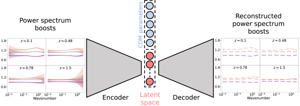
In order to obtain a compressed representation of dark energy power spectrum boosts, we employ a -variational autoencoder (-VAE, [63, 64, 65]). A schematic view of our DE-VAE model is reported in Fig. 1.
In particular, our model is made of two blocks, an encoder and a decoder, both parametrized as three layers of 1-D convolutional neural networks. After each convolutional layer, we apply the same trainable activation function as the one described in Ref. [66] and batch normalization [67], to make training more stable. In the encoder, the convolutional layers are followed by a dense layer with linear activation function, whose output is a set of variables, where is the size of the so-called latent space. These variables represent the mean and the standard deviation of Gaussian distributions. We vary in our analysis from to , and report the corresponding results in Sect. IV.
We sample one point from each latent distribution, and concatenate the latent variables with the five CDM parameters (described in Sect. II and Table 1), to encourage the model to find a representation only of the extension to the CDM model. The concatenated vector is fed through the decoder to obtain a reconstructed version of the input data . The complete model is then trained by optimizing the loss function
| (4) |
where represents the norm, indicates the Kullback-Leibler (KL) divergence between two distributions, is a multivariate standard Gaussian distribution, is a real parameter that we tune to achieve independent latent variables, and is the conditional distribution of the latent variables given the input data. We assume that is the product of independent Gaussian distributions, namely
| (5) |
where the means and standard deviations are the output of the encoder given the input data . With this choice, the KL divergence can be computed analytically as
| (6) |
Our model thus has to balance the two components of the loss: while the first part aims to achieve a good reconstruction error weighted by the uncertainty on the power spectrum boost, the second piece encourages a disentangled latent space, namely a set of independent latent variables, each carrying information about the relevant parameters used to predict the boosts.
The training procedure is analogous to Refs. [68, 69]. We set a batch size of 256, and a starting learning rate of ; we train the model until the validation loss does not improve for 50 consecutive epochs, then decrease the learning rate by a factor of 10, and repeat until the learning rate reaches . Our model is trained using the Adam optimizer [70].
To quantify the dependence between the latent variables and the cosmological parameters, we estimate their mutual information (MI), an information-theoretic measure of the dependence between random variables. Given two random variables with joint probability density , their MI is defined as
| (7) |
where and indicate the marginal distributions, and indicates the natural logarithm, so that MI is measured in natural units (nat). The MI between two variables is zero if and only if the two variables are independent; we refer the reader to Ref. [71] for a complete review of MI and its properties. We employ the GMM-MI library [72], which provides a robust and efficient estimator of MI and includes the uncertainty due to the finite sample size, to obtain MI estimates. We also use GMM-MI to ensure that the latent variables are disentangled: we tune until we reach a MI between latent variables of nat or less. Finally, in the case we further search for an explicit connection between the latent variable and the parameters using symbolic regression, which fits multiple analytic equations to the data through genetic algorithms, as implemented in the PySR library [73].
IV Results
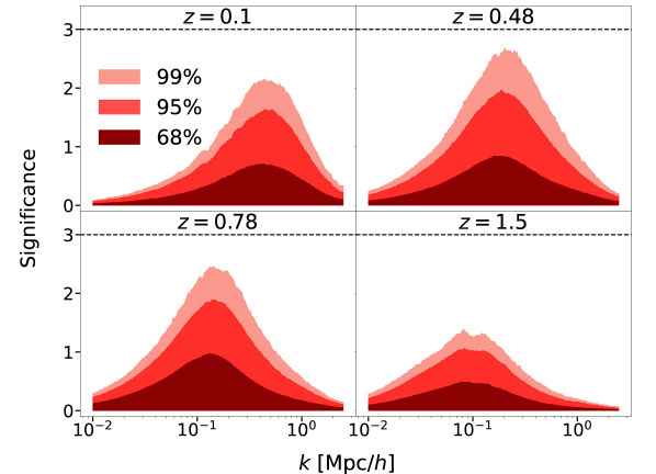
We first report the accuracy of the reconstructed test power spectra when varying the number of latent variables from to . We compute the predicted spectrum by multiplying the output of the decoder, considered noiseless, by ; we then compare the predicted and true power spectra, assuming the uncertainty on the power spectra to be as in Eq. (3). In Fig. 2, we show the 68, 95 and 99 percentiles of the statistical significance,
| (8) |
which represents the accuracy of the prediction in units of the power spectrum error across the test set, with given by Eq. (3). We also ensure that when the latent variables are disentangled, i.e. that their MI is nat or less. Even in the case , we encourage a regularized latent space by setting .
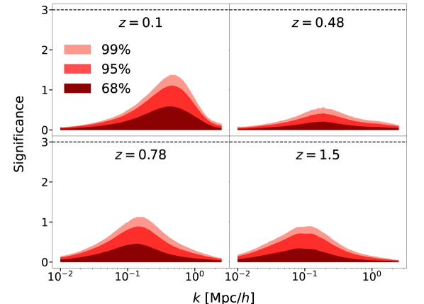
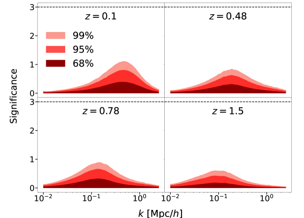

The trained model has a similar performance in all three cases. With one latent variable (, top panel), the percentile plot shows that 95% of the model predictions fall within less than 2 of the observational error for all wavenumbers and redshift bins, with a particularly good performance at . Adding a second latent variable (, middle panel) only marginally improves the model accuracy, which is consistent with the case of three latent variables (, bottom panel). This suggests that adding a third independent latent variable has no impact on the model’s performance: this is in line with the expectations, given that only two additional parameters are used to generate the training data.
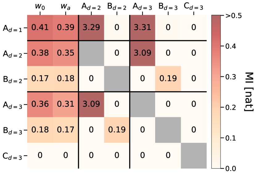
To further interpret these results, in Fig. 3 we report the MI values between the latent variables, and between the latent variables and the dynamical dark energy parameters and . We refer to each latent variable as A, B or C, with a subscript to indicate the dimensionality of the latent space. In the case with , the single latent variable Ad=1 shows a high MI (i.e. significantly higher than 0) with both and , suggesting that Ad=1 carries information on a combination of the two dark energy parameters. This single variable is effectively capable of predicting dynamical dark energy power spectra, with 95% of the predictions falling within 1 of the observational error, increasing to 99% for , as we showed in the upper panel of Fig. 2; we further explore the links between these variables in Sect. IV.1. When training a model with two disentangled latents (Ad=2 and Bd=2), these show a significant MI with both and , with Ad=2 in particular capturing most of the information content. Moreover, Ad=2 has a high MI with Ad=1: this hints at the fact that, when allowing an extra latent variable, the model only learns small corrections on top of the model, as demonstrated by the slightly improved accuracy in the middle panel of Fig. 2 as well. Training a model with a third disentangled latent variable (Cd=3) shows no advantage, since Cd=3 carries no information content about the DE parameters, and is completely independent from all other latent variables. This is confirmed in the bottom panel of Fig. 2, where we show that adding a third latent variable has minimal impact on the accuracy of the prediction of the model.
IV.1 Symbolic regression in latent space
We further investigate the link between the dynamical DE parameters (, ) and the single latent variable Ad=1 using symbolic regression. Without a direct link, given and one would need to create the corresponding power spectrum boost and pass it through the encoder to get the corresponding latent variable. By obtaining an explicit equation, we can both bypass the encoder (which we could achieve with another neural network, too), and reuse the parametrization in other contexts, e.g. for studies looking at other observables beyond the power spectrum, as well as for the development of new theoretical models.
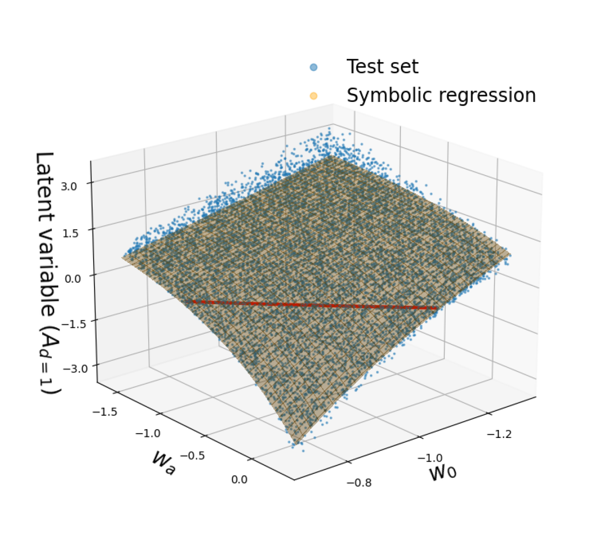
We fit PySR with default parameters on a subset of training data points; we tested that the results do not change when increasing the number of iterations, or when using more data. The best equation we obtain according to the PySR score (0.92 on the test set), which balances the equation’s accuracy and its complexity, is
| (9) |
Note that we have manually rescaled the equation so that, for CDM, . We show the 3D distribution of points for the test set, together with the graph of Eq. (9), in Fig. 4. If we use this equation to predict the value of the latent variable instead of the encoder, the 99% level of the power spectrum predictions can reach up to 5 deviations for the test set described in Table 1; this is to be expected, since symbolic regression tends to sacrifice accuracy in favor of simpler expressions [73]. However, if we restrict ourselves to spectra generated within three standard deviations of the Planck best-fit values (instead of five as the training and test data)666In this case as well, we further limit the ranges of and to and standard deviations, respectively, to avoid numerical instabilities, as we describe in Table 1., we show that this equation actually achieves an acceptable performance, with the percentile accuracy shown in Fig. 5. We also tested that we obtain the same equation if we allow all parameters (CDM+DE) to be given as input variables to predict Ad=1, further confirming that the latent variable only depends on the DE parameters.
V Discussion and outlook
Using our DE-VAE framework, we demonstrated that a single variable is sufficient to accurately predict the matter power spectrum for a particular beyond-CDM model with two additional free parameters. The architecture benefits from its representation learning formulation, which allows us to explore the lower-dimensional latent space and obtain further insight on the nature of the training data. We showcased the use of mutual information as an effective tool to interpret the latent space; moreover, we employed symbolic regression (SR) to obtain an analytic equation linking the cosmological parameters with the latent variable. We envision that our framework can be employed and extended in the following ways.
-
•
Given observational constraints on the matter power spectrum, it is possible to use the DE-VAE decoder within a Markov chain Monte Carlo (MCMC) algorithm to sample the posterior distribution of the latent space (and CDM) parameters, and thus effectively classify the observed spectrum as either in agreement with CDM or not. The value of the latent variable corresponding to CDM can be obtained by passing constant unitary boosts at all redshifts and wavenumbers through the encoder. It would then be straightforward to constrain the latent parameter Ad=1 and assess the statistical significance of any deviations from CDM in latent space.
-
•
The particular latent variable we found with DE-VAE and the corresponding parametrization obtained using SR are optimized for a Euclid-like power spectrum analysis, and capture a particular degeneracy between and in predicting matter power spectra (indicated in red in Fig. 4). This variable can be interpreted in the same vein as , i.e. as a parameter constructed to be particularly well-constrained by a certain dataset. Given that our neural architecture is easily adaptable to different input data, it will be therefore interesting to train our framework on other probes (e.g. on CMB spectra or weak lensing maps). This could yield a latent variable capturing an orthogonal degeneracy with respect to the one we found in this work, and therefore highlight which summary statistics should be targeted to break degeneracies when constraining beyond-CDM models. By analyzing different datasets and considering sky maps rather than 2-point functions, we aim to obtain results which are complementary with respect to the matter power spectrum, as well as retain the information that is lost when compressing the full field into summary statistics [42]. In turn, this can inform the development of future cosmological missions, that could then target these particular parameters and probes to maximize their performance.
-
•
By showcasing the validity of our approach with a single model for which the underlying ground truth is known, we anticipate being able to train an analogous model on a broader variety of spectra obtained assuming different beyond-CDM models, including Hu-Sawicki [74] and dark sector interactions [75], to be used as training data. The power spectrum predictions for these models can be efficiently obtained with the ReACT package [76, 77], or the corresponding emulator [78]. In this way, we expect to capture a common low-dimensional parametrization of a multitude of beyond-CDM scenarios; in turn, this can be used to facilitate the exploration of beyond-CDM models when performing MCMC analyses, and inform the theoretical development of models which try to unify these different extensions.
VI Conclusions
We developed DE-VAE, a framework to search for a compressed representation of beyond-CDM ( cold dark matter) models using representation learning. As a first proof-of-concept study, we focused on dynamical dark energy (DE) as a straightforward extension to the CDM cosmological model. In particular, we considered the archetypal two-variable parametrization of the DE equation of state, and produced the corresponding matter power spectrum boosts as in Eq. (1). These boosts were used as training data of a -variational autoencoder (-VAE) model, summarized in Fig. 1, where we encouraged a -dimensional disentangled compressed representation independent from CDM parameters.
We found that a single latent variable, in combination with five CDM parameters, can predict the power spectra of dynamical DE at different redshifts and up to /Mpc within a (2) error for 95% (99%) of the data; the error, reported in Eq. (3), is computed combining cosmic variance, shot noise and possible systematic effects for a Stage IV-like survey. This single latent variable shows a high mutual information (MI) with the parameters of the DE equation of state, confirming that the DE-VAE has learned a meaningful representation of the boosts. Adding a second independent latent variable only marginally improves the prediction accuracy, with both latent variables showing a significant MI with the DE parameters. Finally, we trained a model with and showed that the third independent latent variable has no MI with other latent variables and with the DE parameters, confirming that it has no significant impact on the prediction accuracy. In the case, we also demonstrated the use of symbolic regression to obtain an explicit equation linking the DE parameters and the latent variable, which can be used to facilitate the power spectrum prediction by skipping the encoder compression, and which sheds further light on the nature of the latent variable.
We highlighted a range of applications and future developments of our framework. To mention a few, these include applying DE-VAE to different cosmological datasets, to explore which probes should be targeted by next-generation surveys to break parameter degeneracies, as well as training the architecture on multiple extensions of CDM, to shed light on their common aspects and inform the development of the underlying theories. We will explore these avenues in future work. The DE-VAE architecture and the data generated to train and test the model are available upon request.
Acknowledgements.
We are grateful to Benjamin Bose and Benjamin Hertzsch for their feedback on this work. DP and LL were supported by a Swiss National Science Foundation (SNSF) Professorship grant (No. 202671). DP was also supported by the SNSF Sinergia grant CRSII5_193716 “Robust Deep Density Models for High-Energy Particle Physics and Solar Flare Analysis (RODEM)”. The computations underlying this work were performed on the Baobab cluster at the University of Geneva.References
- Bull et al. [2016] P. Bull, Y. Akrami, J. Adamek, T. Baker, E. Bellini, J. Beltrán Jiménez, E. Bentivegna, S. Camera, S. Clesse, J. H. Davis, et al., Beyond CDM: Problems, solutions, and the road ahead, Physics of the Dark Universe 12, 56 (2016), arXiv:1512.05356 [astro-ph.CO] .
- Planck Collaboration et al. [2020] Planck Collaboration, N. Aghanim, Y. Akrami, M. Ashdown, J. Aumont, C. Baccigalupi, M. Ballardini, A. J. Banday, R. B. Barreiro, N. Bartolo, and others., Planck 2018 results. VI. Cosmological parameters, A&A 641, A6 (2020), arXiv:1807.06209 [astro-ph.CO] .
- Martin [2012] J. Martin, Everything you always wanted to know about the cosmological constant problem (but were afraid to ask), Comptes Rendus Physique 13, 566 (2012), arXiv:1205.3365 [astro-ph.CO] .
- Riess et al. [2022] A. G. Riess, W. Yuan, L. M. Macri, D. Scolnic, D. Brout, S. Casertano, D. O. Jones, Y. Murakami, G. S. Anand, L. Breuval, et al., A Comprehensive Measurement of the Local Value of the Hubble Constant with 1 km s-1 Mpc-1 Uncertainty from the Hubble Space Telescope and the SH0ES Team, ApJ 934, L7 (2022), arXiv:2112.04510 [astro-ph.CO] .
- Heymans et al. [2021] C. Heymans, T. Tröster, M. Asgari, C. Blake, H. Hildebrandt, B. Joachimi, K. Kuijken, C.-A. Lin, A. G. Sánchez, J. L. van den Busch, et al., KiDS-1000 Cosmology: Multi-probe weak gravitational lensing and spectroscopic galaxy clustering constraints, A&A 646, A140 (2021), arXiv:2007.15632 [astro-ph.CO] .
- Abbott et al. [2023a] T. M. C. Abbott, M. Aguena, A. Alarcon, O. Alves, A. Amon, F. Andrade-Oliveira, M. Asgari, S. Avila, D. Bacon, K. Bechtol, et al. (Dark Energy Survey and Kilo-Degree Survey Collaboration), DES Y3 + KiDS-1000: Consistent cosmology combining cosmic shear surveys, arXiv e-prints , arXiv:2305.17173 (2023a), arXiv:2305.17173 [astro-ph.CO] .
- Ivezić et al. [2019] Ž. Ivezić, S. M. Kahn, J. A. Tyson, B. Abel, E. Acosta, R. Allsman, D. Alonso, Y. AlSayyad, S. F. Anderson, J. Andrew, et al., LSST: From Science Drivers to Reference Design and Anticipated Data Products, ApJ 873, 111 (2019), arXiv:0805.2366 [astro-ph] .
- Laureijs et al. [2011] R. Laureijs, J. Amiaux, S. Arduini, J. L. Auguères, J. Brinchmann, R. Cole, M. Cropper, C. Dabin, L. Duvet, A. Ealet, et al., Euclid Definition Study Report, arXiv e-prints , arXiv:1110.3193 (2011), arXiv:1110.3193 [astro-ph.CO] .
- Spergel et al. [2015] D. Spergel, N. Gehrels, C. Baltay, D. Bennett, J. Breckinridge, M. Donahue, A. Dressler, B. S. Gaudi, T. Greene, O. Guyon, et al., Wide-Field InfrarRed Survey Telescope-Astrophysics Focused Telescope Assets WFIRST-AFTA 2015 Report, arXiv e-prints , arXiv:1503.03757 (2015), arXiv:1503.03757 [astro-ph.IM] .
- Ade et al. [2019] P. Ade, J. Aguirre, Z. Ahmed, S. Aiola, A. Ali, D. Alonso, M. A. Alvarez, K. Arnold, P. Ashton, J. Austermann, et al., The Simons Observatory: science goals and forecasts, Journal of Cosmology and Astroparticle Physics 2019 (02), 056–056.
- Copeland et al. [2006] E. J. Copeland, M. Sami, and S. Tsujikawa, Dynamics of Dark Energy, International Journal of Modern Physics D 15, 1753 (2006), arXiv:hep-th/0603057 [hep-th] .
- Clifton et al. [2012] T. Clifton, P. G. Ferreira, A. Padilla, and C. Skordis, Modified gravity and cosmology, Phys. Rep. 513, 1 (2012), arXiv:1106.2476 [astro-ph.CO] .
- Koyama [2016] K. Koyama, Cosmological tests of modified gravity, Reports on Progress in Physics 79, 046902 (2016), arXiv:1504.04623 [astro-ph.CO] .
- Joyce et al. [2015] A. Joyce, B. Jain, J. Khoury, and M. Trodden, Beyond the cosmological standard model, Phys. Rep. 568, 1 (2015), arXiv:1407.0059 [astro-ph.CO] .
- Joyce et al. [2016] A. Joyce, L. Lombriser, and F. Schmidt, Dark Energy Versus Modified Gravity, Annual Review of Nuclear and Particle Science 66, 95 (2016), arXiv:1601.06133 [astro-ph.CO] .
- Ishak [2019] M. Ishak, Testing general relativity in cosmology, Living Reviews in Relativity 22, 1 (2019), arXiv:1806.10122 [astro-ph.CO] .
- Di Valentino et al. [2021] E. Di Valentino, O. Mena, S. Pan, L. Visinelli, W. Yang, A. Melchiorri, D. F. Mota, A. G. Riess, and J. Silk, In the realm of the Hubble tension-a review of solutions, Classical and Quantum Gravity 38, 153001 (2021), arXiv:2103.01183 [astro-ph.CO] .
- Williams et al. [2004] J. G. Williams, S. G. Turyshev, and D. H. Boggs, Progress in Lunar Laser Ranging Tests of Relativistic Gravity, Phys. Rev. Lett. 93, 261101 (2004).
- Schlamminger et al. [2008] S. Schlamminger, K.-Y. Choi, T. A. Wagner, J. H. Gundlach, and E. G. Adelberger, Test of the Equivalence Principle Using a Rotating Torsion Balance, Phys. Rev. Lett. 100, 041101 (2008).
- Wagner et al. [2012] T. A. Wagner, S. Schlamminger, J. H. Gundlach, and E. G. Adelberger, Torsion-balance tests of the weak equivalence principle, Classical and Quantum Gravity 29, 184002 (2012).
- Will [2014] C. M. Will, The Confrontation between General Relativity and Experiment, Living Reviews in Relativity 17, 4 (2014), arXiv:1403.7377 [gr-qc] .
- Peebles [2005] P. J. E. Peebles, Testing General Relativity on the Scales of Cosmology , in General Relativity and Gravitation (World Scientific, 2005).
- Vainshtein [1972] A. Vainshtein, To the problem of nonvanishing gravitation mass, Physics Letters B 39, 393 (1972).
- Babichev and Deffayet [2013] E. Babichev and C. Deffayet, An introduction to the Vainshtein mechanism, Classical and Quantum Gravity 30, 184001 (2013), arXiv:1304.7240 [gr-qc] .
- Babichev et al. [2009] E. Babichev, C. Deffayet, and R. Ziour, -Mouflage gravity, International Journal of Modern Physics D 18, 2147 (2009), https://doi.org/10.1142/S0218271809016107 .
- Khoury and Weltman [2004] J. Khoury and A. Weltman, Chameleon cosmology, Phys. Rev. D 69, 044026 (2004), arXiv:astro-ph/0309411 [astro-ph] .
- Hinterbichler and Khoury [2010] K. Hinterbichler and J. Khoury, Screening Long-Range Forces through Local Symmetry Restoration, Phys. Rev. Lett. 104, 231301 (2010).
- Lombriser [2018] L. Lombriser, Parametrizations for tests of gravity, International Journal of Modern Physics D 27, 1848002 (2018), arXiv:1908.07892 [astro-ph.CO] .
- Hu and Sawicki [2007a] W. Hu and I. Sawicki, Parametrized post-Friedmann framework for modified gravity, Phys. Rev. D 76, 104043 (2007a).
- Zhang et al. [2007] P. Zhang, M. Liguori, R. Bean, and S. Dodelson, Probing Gravity at Cosmological Scales by Measurements which Test the Relationship between Gravitational Lensing and Matter Overdensity, Phys. Rev. Lett. 99, 141302 (2007).
- Amendola et al. [2008] L. Amendola, M. Kunz, and D. Sapone, Measuring the dark side (with weak lensing), J. Cosmology Astropart. Phys 2008, 013 (2008), arXiv:0704.2421 [astro-ph] .
- Bertschinger and Zukin [2008] E. Bertschinger and P. Zukin, Distinguishing modified gravity from dark energy, Phys. Rev. D 78, 024015 (2008).
- Bean and Tangmatitham [2010] R. Bean and M. Tangmatitham, Current constraints on the cosmic growth history, Phys. Rev. D 81, 083534 (2010).
- Pogosian et al. [2010] L. Pogosian, A. Silvestri, K. Koyama, and G.-B. Zhao, How to optimally parametrize deviations from general relativity in the evolution of cosmological perturbations, Phys. Rev. D 81, 104023 (2010).
- Song et al. [2010] Y.-S. Song, L. Hollenstein, G. Caldera-Cabral, and K. Koyama, Theoretical priors on modified growth parametrisations, Journal of Cosmology and Astroparticle Physics 2010 (04), 018.
- Huterer and Starkman [2003] D. Huterer and G. Starkman, Parametrization of Dark-Energy Properties: A Principal-Component Approach, Phys. Rev. Lett. 90, 031301 (2003).
- Crittenden et al. [2009] R. G. Crittenden, L. Pogosian, and G.-B. Zhao, Investigating dark energy experiments with principal components, J. Cosmology Astropart. Phys 2009, 025 (2009), arXiv:astro-ph/0510293 [astro-ph] .
- Zhao et al. [2009] G.-B. Zhao, L. Pogosian, A. Silvestri, and J. Zylberberg, Cosmological Tests of General Relativity with Future Tomographic Surveys, Phys. Rev. Lett. 103, 241301 (2009).
- Hojjati et al. [2012] A. Hojjati, G.-B. Zhao, L. Pogosian, A. Silvestri, R. Crittenden, and K. Koyama, Cosmological tests of general relativity: A principal component analysis, Phys. Rev. D 85, 043508 (2012).
- Asaba et al. [2013] S. Asaba, C. Hikage, K. Koyama, G.-B. Zhao, A. Hojjati, and L. Pogosian, Principal component analysis of modified gravity using weak lensing and peculiar velocity measurements, Journal of Cosmology and Astroparticle Physics 2013 (08), 029.
- Schmelzle et al. [2017] J. Schmelzle, A. Lucchi, T. Kacprzak, A. Amara, R. Sgier, A. Réfrégier, and T. Hofmann, Cosmological model discrimination with Deep Learning, arXiv e-prints , arXiv:1707.05167 (2017), arXiv:1707.05167 [astro-ph.CO] .
- Peel et al. [2019] A. Peel, F. Lalande, J.-L. Starck, V. Pettorino, J. Merten, C. Giocoli, M. Meneghetti, and M. Baldi, Distinguishing standard and modified gravity cosmologies with machine learning, Phys. Rev. D 100, 023508 (2019), arXiv:1810.11030 [astro-ph.CO] .
- Mancarella et al. [2022] M. Mancarella, J. Kennedy, B. Bose, and L. Lombriser, Seeking new physics in cosmology with bayesian neural networks: Dark energy and modified gravity, Phys. Rev. D 105, 023531 (2022).
- Portillo et al. [2020] S. K. N. Portillo, J. K. Parejko, J. R. Vergara, and A. J. Connolly, Dimensionality Reduction of SDSS Spectra with Variational Autoencoders, The Astronomical Journal 160, 45 (2020).
- Sedaghat et al. [2021] N. Sedaghat, M. Romaniello, J. E. Carrick, and F.-X. Pineau, Machines learn to infer stellar parameters just by looking at a large number of spectra, MNRAS 501, 6026 (2021), arXiv:2009.12872 [astro-ph.IM] .
- Sarmiento et al. [2021] R. Sarmiento, M. Huertas-Company, J. H. Knapen, S. F. Sánchez, H. Domínguez Sánchez, N. Drory, and J. Falcón-Barroso, Capturing the Physics of MaNGA Galaxies with Self-supervised Machine Learning, ApJ 921, 177 (2021), arXiv:2104.08292 [astro-ph.GA] .
- Teimoorinia et al. [2022] H. Teimoorinia, F. Archinuk, J. Woo, S. Shishehchi, and A. F. L. Bluck, Mapping the Diversity of Galaxy Spectra with Deep Unsupervised Machine Learning, The Astronomical Journal 163, 71 (2022).
- Lucie-Smith et al. [2022] L. Lucie-Smith, H. V. Peiris, A. Pontzen, B. Nord, J. Thiyagalingam, and D. Piras, Discovering the building blocks of dark matter halo density profiles with neural networks, Phys. Rev. D 105, 103533 (2022).
- Lucie-Smith et al. [2023] L. Lucie-Smith, H. V. Peiris, and A. Pontzen, Explaining dark matter halo density profiles with neural networks, arXiv e-prints , arXiv:2305.03077 (2023), arXiv:2305.03077 [astro-ph.CO] .
- Chevallier and Polarski [2001] M. Chevallier and D. Polarski, Accelerating Universes with Scaling Dark Matter, International Journal of Modern Physics D 10, 213 (2001), arXiv:gr-qc/0009008 [gr-qc] .
- Linder [2003] E. V. Linder, Exploring the Expansion History of the Universe, Phys. Rev. Lett. 90, 091301 (2003), arXiv:astro-ph/0208512 [astro-ph] .
- Menci et al. [2020] N. Menci, A. Grazian, M. Castellano, P. Santini, E. Giallongo, A. Lamastra, F. Fortuni, A. Fontana, E. Merlin, T. Wang, et al., Constraints on Dynamical Dark Energy Models from the Abundance of Massive Galaxies at High Redshifts, ApJ 900, 108 (2020), arXiv:2007.12453 [astro-ph.CO] .
- Abbott et al. [2023b] T. M. C. Abbott, M. Aguena, A. Alarcon, O. Alves, A. Amon, F. Andrade-Oliveira, J. Annis, S. Avila, D. Bacon, E. Baxter, et al. (DES Collaboration), Dark Energy Survey Year 3 results: Constraints on extensions to with weak lensing and galaxy clustering, Phys. Rev. D 107, 083504 (2023b).
- Lewis and Challinor [2011] A. Lewis and A. Challinor, CAMB: Code for Anisotropies in the Microwave Background, Astrophysics Source Code Library, record ascl:1102.026 (2011), ascl:1102.026 .
- Mead et al. [2015] A. J. Mead, J. A. Peacock, C. Heymans, S. Joudaki, and A. F. Heavens, An accurate halo model for fitting non-linear cosmological power spectra and baryonic feedback models, Monthly Notices of the Royal Astronomical Society 454, 1958 (2015), https://academic.oup.com/mnras/article-pdf/454/2/1958/9381114/stv2036.pdf .
- Mead et al. [2016] A. J. Mead, C. Heymans, L. Lombriser, J. A. Peacock, O. I. Steele, and H. A. Winther, Accurate halo-model matter power spectra with dark energy, massive neutrinos and modified gravitational forces, Monthly Notices of the Royal Astronomical Society 459, 1468 (2016), https://academic.oup.com/mnras/article-pdf/459/2/1468/8040273/stw681.pdf .
- Mead et al. [2021] A. J. Mead, S. Brieden, T. Tröster, and C. Heymans, HMcode-2020: Improved modelling of non-linear cosmological power spectra with baryonic feedback, Monthly Notices of the Royal Astronomical Society 502, 1401 (2021), https://academic.oup.com/mnras/article-pdf/502/1/1401/36182229/stab082.pdf .
- Aghanim et al. [2020] N. Aghanim, Y. Akrami, M. Ashdown, J. Aumont, C. Baccigalupi, M. Ballardini, A. J. Banday, R. B. Barreiro, N. Bartolo, S. Basak, et al., Planck 2018 results. VI. Cosmological parameters, A&A 641, A6 (2020), arXiv:1807.06209 [astro-ph.CO] .
- Blanchard et al. [2020] A. Blanchard, S. Camera, C. Carbone, V. F. Cardone, S. Casas, S. Clesse, S. Ilić, M. Kilbinger, T. Kitching, M. Kunz, et al., Euclid preparation. VII. Forecast validation for Euclid cosmological probes, A&A 642, A191 (2020), arXiv:1910.09273 [astro-ph.CO] .
- Feldman et al. [1994] H. A. Feldman, N. Kaiser, and J. A. Peacock, Power-Spectrum Analysis of Three-dimensional Redshift Surveys, ApJ 426, 23 (1994), arXiv:astro-ph/9304022 [astro-ph] .
- Seo and Eisenstein [2007] H.-J. Seo and D. J. Eisenstein, Improved Forecasts for the Baryon Acoustic Oscillations and Cosmological Distance Scale, ApJ 665, 14 (2007), arXiv:astro-ph/0701079 [astro-ph] .
- Zhao [2014] G.-B. Zhao, Modeling the Nonlinear Clustering in Modified Gravity Models. I. A Fitting Formula for the Matter Power Spectrum of f(R) Gravity, ApJS 211, 23 (2014), arXiv:1312.1291 [astro-ph.CO] .
- Kingma and Welling [2014] D. P. Kingma and M. Welling, Auto-Encoding Variational Bayes, in 2nd International Conference on Learning Representations, ICLR 2014, Banff, AB, Canada, April 14-16, 2014, Conference Track Proceedings, edited by Y. Bengio and Y. LeCun (2014).
- Rezende et al. [2014] D. J. Rezende, S. Mohamed, and D. Wierstra, Stochastic backpropagation and approximate inference in deep generative models, in Proceedings of the 31st International Conference on Machine Learning, Proceedings of Machine Learning Research, Vol. 32(2), edited by E. P. Xing and T. Jebara (PMLR, Bejing, China, 2014) pp. 1278–1286.
- Higgins et al. [2017] I. Higgins, L. Matthey, A. Pal, C. P. Burgess, X. Glorot, M. M. Botvinick, S. Mohamed, and A. Lerchner, beta-VAE: Learning Basic Visual Concepts with a Constrained Variational Framework, in 5th International Conference on Learning Representations, ICLR 2017, Toulon, France, April 24-26, 2017, Conference Track Proceedings (OpenReview.net, 2017).
- Alsing et al. [2020] J. Alsing, H. Peiris, J. Leja, C. Hahn, R. Tojeiro, D. Mortlock, B. Leistedt, B. D. Johnson, and C. Conroy, SPECULATOR: Emulating Stellar Population Synthesis for Fast and Accurate Galaxy Spectra and Photometry, The Astrophysical Journal Supplement Series 249, 5 (2020).
- Ioffe and Szegedy [2015] S. Ioffe and C. Szegedy, Batch Normalization: Accelerating Deep Network Training by Reducing Internal Covariate Shift, in Proceedings of the 32nd International Conference on Machine Learning, Proceedings of Machine Learning Research, Vol. 37, edited by F. Bach and D. Blei (PMLR, Lille, France, 2015) pp. 448–456.
- Spurio Mancini et al. [2022] A. Spurio Mancini, D. Piras, J. Alsing, B. Joachimi, and M. P. Hobson, CosmoPower: emulating cosmological power spectra for accelerated Bayesian inference from next-generation surveys, Monthly Notices of the Royal Astronomical Society 511, 1771–1788 (2022).
- Piras and Spurio Mancini [2023] D. Piras and A. Spurio Mancini, CosmoPower-JAX: high-dimensional Bayesian inference with differentiable cosmological emulators, The Open Journal of Astrophysics 6, 20 (2023), arXiv:2305.06347 [astro-ph.CO] .
- Kingma and Ba [2015] D. P. Kingma and J. Ba, Adam: A method for stochastic optimization, in 3rd International Conference on Learning Representations, ICLR 2015, San Diego, CA, USA, May 7-9, 2015, Conference Track Proceedings, edited by Y. Bengio and Y. LeCun (2015).
- Vergara and Estévez [2015] J. R. Vergara and P. A. Estévez, A Review of Feature Selection Methods Based on Mutual Information, arXiv e-prints , arXiv:1509.07577 (2015), arXiv:1509.07577 [cs.LG] .
- Piras et al. [2023] D. Piras, H. V. Peiris, A. Pontzen, L. Lucie-Smith, N. Guo, and B. Nord, A robust estimator of mutual information for deep learning interpretability, Machine Learning: Science and Technology 4, 025006 (2023).
- Cranmer [2023] M. Cranmer, Interpretable Machine Learning for Science with PySR and SymbolicRegression.jl, arXiv e-prints , arXiv:2305.01582 (2023), arXiv:2305.01582 [astro-ph.IM] .
- Hu and Sawicki [2007b] W. Hu and I. Sawicki, Models of cosmic acceleration that evade solar system tests, Phys. Rev. D 76, 064004 (2007b).
- Dvali et al. [2000] G. Dvali, G. Gabadadze, and M. Porrati, 4d gravity on a brane in 5d minkowski space, Physics Letters B 485, 208 (2000).
- Bose et al. [2020] B. Bose, M. Cataneo, T. Tröster, Q. Xia, C. Heymans, and L. Lombriser, On the road to percent accuracy IV: ReACT – computing the non-linear power spectrum beyond CDM, Monthly Notices of the Royal Astronomical Society 498, 4650 (2020), https://academic.oup.com/mnras/article-pdf/498/4/4650/33798567/staa2696.pdf .
- Bose et al. [2023] B. Bose, M. Tsedrik, J. Kennedy, L. Lombriser, A. Pourtsidou, and A. Taylor, Fast and accurate predictions of the non-linear matter power spectrum for general models of Dark Energy and Modified Gravity, Monthly Notices of the Royal Astronomical Society 519, 4780 (2023), https://academic.oup.com/mnras/article-pdf/519/3/4780/48744919/stac3783.pdf .
- Spurio Mancini and Bose [2023] A. Spurio Mancini and B. Bose, On the degeneracies between baryons, massive neutrinos and f(R) gravity in Stage IV cosmic shear analyses, arXiv e-prints , arXiv:2305.06350 (2023), arXiv:2305.06350 [astro-ph.CO] .