Reusing Pretrained Models by Multi-linear Operators for Efficient Training

Abstract

Training large models from scratch usually costs a substantial amount of resources. Towards this problem, recent studies such as bert2BERT and LiGO have reused small pretrained models to initialize a large model (termed the “target model”), leading to a considerable acceleration in training. Despite the successes of these previous studies, they grew pretrained models by mapping partial weights only, ignoring potential correlations across the entire model. As we show in this paper, there are inter- and intra-interactions among the weights of both the pretrained and the target models. As a result, the partial mapping may not capture the complete information and lead to inadequate growth. In this paper, we propose a method that linearly correlates each weight of the target model to all the weights of the pretrained model to further enhance acceleration ability. We utilize multi-linear operators to reduce computational and spacial complexity, enabling acceptable resource requirements. Experiments demonstrate that our method can save 76% computational costs on DeiT-base transferred from DeiT-small, which outperforms bert2BERT by +12.0% and LiGO by +20.7%, respectively.

1 Introduction

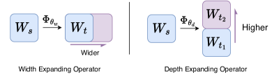
Figure 1: Expanding operators. $W_{s}$ and $W_{t}$ mean small pretrained and target weights, respectively. $\Phi_{\theta_{w}}$ and $\Phi_{\theta_{d}}$ denote width and depth expanding operators with parameters $\theta_{w}$ and $\theta_{d}$.

Transformers [47] have recently achieved great successes in various scenarios [11, 4, 20]. Generally, Transformers tend to be larger for more expressive power and better performance (e.g., ViT-G [6] and GPT-3 [3]). As the size of models continues to grow, training Transformers takes longer and can result in higher CO₂ emissions, which conflicts with the principles of Green AI [43]. Thus, training Transformers efficiently is crucial not only for financial gain but also for environmental sustainability [5]. To achieve efficient training, it is a wise option to grow a pretrained small model into a larger one, since the pretrained small model has already learned knowledge from the data, which allows for faster training compared to starting from scratch. [13]. Moreover, there are numerous pretrained models that are easily accessible [53], reducing the cost of utilizing a smaller pretrained model. Furthermore, empirical evidence shows that Transformers have inductive biases that facilitate scaling fitting [42, 22]. This demonstrates the feasibility of learning from pretrained models [53].

The concept of reusing pretrained models essentially involves exploring the efficient mapping from the pretrained model to the target model. This mapping process can be represented as linear growth operators, as depicted in Figure 1. One viable approach to mapping is to leverage knowledge from other weights. For instance, StackBERT [13] utilizes low-layer information to construct new higher layers, by duplicating layers to increase depth during training epochs. bert2BERT [5] expands width through the expanding operator of Net2Net [7]. Differently, bert2BERT utilizes weights of neighbor layers for enhancing the ability, which also shows the benefit of taking knowledge from other weights. Moreover, distinct from the aforementioned research directly employing a fixed operator, LiGO [53] trains expanding operators which are tied with layers to achieve superior transfer accuracy by considering knowledge from other layers, which is advantageous for training efficiency. However, they neglect the potential connectivity between models.

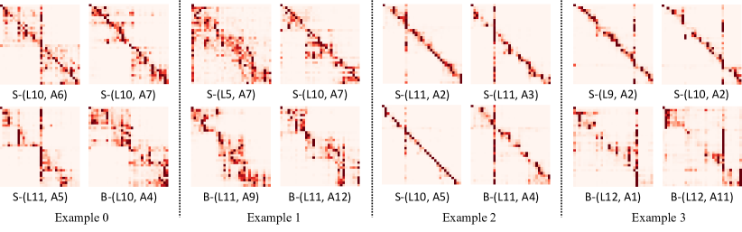
Figure 2: Attention pattern maps between BERT-Small (shorted as “S”) and BERT-Base (shorted as “B”) in four examples. “L” represents the layer index, while “A” denotes the index of the attention head. For example, “S-(L10, A6)” denotes the attention map from layer 10, head 6 of the BERT-Small model. The examples are derived from different sentences. In each example, we can observe the similarities of attention maps in both inter-layer and intra-layer connections, even across different scaled models.

Potential Connectivity between Models. The attention maps of BERT, as depicted in Figure 2, indicate that there are similarities not only in the weights of the same or different layers, but also across different models. These similarities suggest that we can leverage a full mapping transformation to capture this correlation in both inter-layer and intra-layer connections, even across different scaled models. By doing so, we can reuse the parameters of pretrained small models and accelerate the training of larger models. However, previous studies have overlooked the overall network connectivity and have instead expanded each weight through partial mapping transformation. For instance, Net2Net [7] only considers preserving functionality by transforming weights individually, while bert2BERT [5] increases model width head by head in Transformers. On the other hand, LiGO [53] primarily focuses on extending the weights of the same type (e.g., query, key, and value in Transformers), which heavily affects the performance of the transferred models.

Multi-linear Operators. Based on the above observations, we propose mapping the entire pretrained model to each weight of the target model, instead of employing a partial transformation. This approach can ensure high expressive power, promoting the potential connectivity in models for better training efficiency. However, the completed mapping has a huge parameter tensor, occupying an enormous space (see Section 3.2). To address this issue, we propose Mango, a multi-linear structure (i.e., tensor ring [33, 52, 51]), which decomposes the large mapping tensor into four smaller tensors that are bonded by ranks to construct multi-linear operators. Mango allows for efficient training by reducing the space required for the mapping tensor. Formally, Mango can be considered as a generalization of LiGO and bert2BERT (see Section 3.3). By using the full mapping approach, Mango can save 76% computational costs on DeiT-base transferred from DeiT-small, which outperforms bert2BERT [5] by +12.0% and LiGO [53] by +20.7%, respectively.

2 Related Work

Efficient Training from Scratches. Model scratches can be roughly regarded as models without knowledge priors. Some training strategies for scratches are universal and orthogonal to our method. For example, Adam [23] and large-batch size training [66] accelerate the training process from angles of optimizer and magnitude of input data, respectively. Wang et al. [50] enable the training of very deep neural networks with limited computational resources via a technique called active memory. Shoeybi et al. [45] use mixed precision training to assist training. Low-rank methods benefit training for less memory and time [21]. Wu et al. [59] take notes of rare words for better data efficiency. Dropping layers [68], knowledge inheritance [38], and merging tokens [2] are also efficient methods for training. Another line of work [13, 63, 14, 44] is termed progressive training, which gradually increases the model size within the training process for training efficiency. Li et al. [27] employ a neural architecture search (NAS) method to search optimal sub-networks for progressive training on ViTs. Xia et al. [60] suggest a three-phase progressive training regime to achieve a good trade-off between training budget and performance. Wang et al. [55] introduces a novel curriculum learning approach for training efficiency through firstly learning simpler patterns, then progressively introducing more complex patterns.

Efficient Training from Pretrained Models. Pretrained models usually contain abundant data knowledge, which is helpful for training [32]. By preserving the function of a pretrained model while expanding the model size, it is feasible to give the corresponding larger model an initial state with high performance. Net2Net [7] is the first work to propose the concept of function-preserving transformations by expanding width by splitting neurons and growing depth with identity layers. However, Net2Net splits neurons randomly. Towards this problem, a series of studies [56, 58, 49, 57] propose to select the optimal subset of neurons to be split by utilizing functional steepest descent. bert2BERT [5] expands small transformers by following the function preserving idea. Recently, LiGO [53] utilizes a trainable linear operator to learn a good expanding formula. Different from these prior studies, our method tries to implement a full mapping that achieves comprehensive utilization of the whole smaller model.

Neural Network Initialization. Our method is related to neural network initialization techniques. Xavier [12] and Kaiming [16] initialization aim to control input variance equal to that of output. Generalizing Xavier and Kaiming methods, a universal weight initialization paradigm proposed by Pan et al. [34] can be widely applicable to arbitrary Tensorial CNNs. In addition, Hardt and Ma [15] has shown theoretically that network training benefits from maintaining identity, particularly for improving the efficiency of residual networks. Fixup [67] and ZerO [70] both set residual stem to 0 (not residual connections) to ensure the identity of signals, thereby successfully initializing ResNets. SkipInit [8] replaces Batch Normalization with a multiplier whose value is 0. ReZero [1], on the other hand, adds extra parameters of value $0$ to maintain identity, resulting in faster convergence. IDInit is an initialization approach to keep the identity matrix for stable training of networks [36]. In comparison, our work explores fully reusing smaller pretrained models as efficient initialization.

Low-rank Techniques in Neural Networks. Low-rank methods are feasible for reducing spatial and temporal complexities in neural networks [52, 35, 62]. For example, Idelbayev and Carreira-Perpiñán [19] uses matrix decomposition to compress convolutional neural networks (CNNs) for faster inference. LoRA [17] applies low-rank matrices for fine-tuning large language models (LLMs) in affordable resources. As a parameter-efficient tuning (PETuning) method [69] for federated learning, FedPara [18] utilizes the Hadamard product on low-rank parameters for reducing communication time in federated learning. Pan et al. [33] and Li et al. [28] use tensor ring decomposition for reducing the size of neural networks. Tucker decomposition and block-term Tucker decomposition have been used in T-Net and BT-layers  [24, 64] for improving the model performance, respectively. Ma et al. [30] apply block-term Tucker to compress Transformers. Yin et al. [65] propose to use ADMM to optimize tensor training to achieve better compression and performance. These techniques have built a solid foundation for our work to implement multi-linear transformation for transferring knowledge from pretrained models to target models.

3 Mango Operator

This section presents the proposed Mango operator. First, we provide an overview of the tensor diagram, the concept of the tensor ring matrix product operator (TR-MPO), and the formulation of Transformer architecture in Sec. 3.1. Next, we delve into the details of the proposed multi-linear mapping operator (i.e., Mango) in Sec. 3.2. Finally, we compare Mango with recent advances in terms of tensor diagrams in Sec. 3.3.

3.1 Preliminary

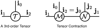
Figure 3: Tensor diagram instances.

Tensor Diagram. Tensor decomposition is a technique that involves splitting a tensor into multiple smaller tensors, typically more than the two matrices that result from matrix factorization. To better illustrate the interactions among multiple tensors, tensor diagrams are often used. A tensor diagram is composed of two primary elements: a tensor vertex and a tensor contraction. A tensor vertex represents a tensor, and its order is determined by the number of edges connected to it. Each edge is assigned an integer that indicates the dimension of the corresponding mode. As shown in Figure 3, a 3rd-order tensor $\bm{\mathcal{T}}\in\mathbb{R}^{\mathbf{i}_{0}\times\mathbf{i}_{1}\times\mathbf{i}_{2}}$ can be drawn as a circle with three edges. The process of taking the inner product of two tensors on their matching modes is called tensor contraction. For example, Two tensors, $\bm{\mathcal{M}}\in\mathbb{R}^{\mathbf{i}_{0}\times\mathbf{i}_{1}\times\mathbf{i}_{2}}$ and $\bm{\mathcal{N}}\in\mathbb{R}^{\mathbf{j}_{0}\times\mathbf{j}_{1}\times\mathbf{j}_{2}}$, can be contracted in corresponding positions to form a new tensor of $\mathbb{R}^{\mathbf{i}_{0}\times\mathbf{i}_{1}\times\mathbf{j}_{2}\times\mathbf{j}_{3}}$, when they have equal dimensions: $\mathbf{i}_{2}=\mathbf{j}_{0}\triangleq e_{0}$. The contraction operation can be formulated as

$$(\bm{\mathcal{M}}\times_{2}^{0}\bm{\mathcal{N}})_{i_{0},i_{1},j_{2},j_{3}}=\sum_{m=0}^{e_{0}-1}\bm{\mathcal{M}}_{i_{0},i_{1},m}\bm{\mathcal{N}}_{m,j_{2},j_{3}}.$$ (1)

The tensor diagram is an elegant tool for succinctly visualizing and manipulating multi-dimensional arrays or tensors. By representing tensor operations as networks of nodes and edges, these diagrams provide an intuitive way to understand the underlying mathematical operations and their interactions. As a result, we have chosen to use tensor diagrams to illustrate our method and to analyze the connections between our approach and prior studies.

Tensor Ring Matrix Product Operator (TR-MPO). TR-MPO means tensor ring (TR) of an MPO [37] format. Given a $2N$-order tensor $\bm{\mathcal{X}}\in\mathbb{R}^{I_{1}\times J_{1}\times I_{2}\times J_{2}\ldots I_{N}\times J_{N}}$, its TR-MPO decomposition can be mathematically expressed as

$$\bm{\mathcal{X}}_{i_{1},j_{1},i_{2},j_{2}\ldots,i_{N},j_{N}}\approx\sum_{r_{1},r_{2},\ldots,r_{N}=1}^{R_{1},R_{2},\ldots,R_{N}}\bm{\mathcal{G}}^{(1)}_{r_{1},i_{1},j_{1},r_{2}}\bm{\mathcal{G}}^{(2)}_{r_{2},i_{2},j_{2},r_{3}}\bm{\mathcal{G}}^{(3)}_{r_{3},i_{3},j_{3},r_{4}}\cdots\bm{\mathcal{G}}^{(N)}_{r_{N},i_{N},j_{N},r_{1}},$$ (2)

where $\{R_{1},R_{2},\ldots,R_{N}\}$ denote the ranks, $\bm{\mathcal{G}}^{(n)}\in\mathbb{R}^{R_{n}\times I_{n}\times I_{n}\times R_{n+1}}$ denotes a 4th-order core tensor and $R_{1}=R_{N+1}$, which indicates ring-like structure.

Transformer Architecture. The Transformer [47] is a deep learning architecture that has revolutionized the artificial intelligence field including computer vision (CV) and natural language processing (NLP). As shown in Figure 4, a Transformer block consists of two main sub-layers: the multi-head self-attention (MHSA) layer and the feed-forward neural network (FFN) layer.

(1) MHSA Layer. The MHSA layer in the Transformer block computes the attention scores between each input element and every other element, allowing the model to attend to different parts of the input sequence during processing. Inputs of MHSA are query matrix $\mathbf{Q}\in\mathbb{R}^{I}$, key matrix $\mathbf{K}\in\mathbb{R}^{I}$ and value matrix $\mathbf{V}\in\mathbb{R}^{I}$ with parameters $\mathbf{W}^{Q}\in\mathbb{R}^{I\times O},\mathbf{W}^{K}\in\mathbb{R}^{I\times O},\mathbf{W}^{V}\in\mathbb{R}^{I\times O},\mathbf{W}^{O}\in\mathbb{R}^{I\times O}$. Usually, it constrains $I=O$. Moreover, MHSA separates these parameters into $n$ heads: $\{\mathbf{W}^{Q,i}\}^{n},\{\mathbf{W}^{K,i}\}^{n},\{\mathbf{W}^{V,i}\}^{n},\{\mathbf{W}^{O,i}\}^{n}$. The MHSA mechanism can be formulated as follows:

$$\operatorname{Att}_{i}(\mathbf{Q},\mathbf{K},\mathbf{V})=\operatorname{softmax}\left(\frac{\mathbf{Q}\mathbf{W}^{Q,i}(\mathbf{K}\mathbf{W}^{K,i})^{T}}{\sqrt{d_{k}}}\right)\mathbf{V}\mathbf{W}^{V,i}\mathbf{W}^{{O,i}^{T}},$$

$$\operatorname{MHSA}((\mathbf{Q},\mathbf{K},\mathbf{V}))=\sum^{n}_{i=1}{\operatorname{Att}_{i}(\mathbf{Q},\mathbf{K},\mathbf{V})},$$ (3)

where $d_{k}$ is the dimensionality of the key vectors. The self-attention mechanism is performed multiple times in parallel, each time using a different set of learned parameters $\mathbf{W}^{Q,i}$, $\mathbf{W}^{K,i}$, and $\mathbf{W}^{V,i}$ to compute multiple "heads" of attention. The resulting attention heads are linearly transformed by a learned weight matrix $\mathbf{W}^{O,i}$ to produce the output. At last, MHSA concatenates the output as the final result of the MHSA layer.

(2) FFN Layer. The FFN layer in the Transformer block is responsible for applying a non-linear transformation to the output of the self-attention layer. $\mathbf{X}\in\mathbb{R}^{I}$ is the input. The weights are $\mathbf{W}^{IN}\in\mathbb{R}^{I\times kO}$ and $\mathbf{W}^{OUT}\in\mathbb{R}^{kI\times O}$, where usually $I=O$ and $k$ is a ratio that is often set to 4. The FFN layer can be formulated as

$$\operatorname{FFN}(\mathbf{X})=\operatorname{GeLU}(\mathbf{X}\mathbf{W}^{IN})\mathbf{W}^{OUT}.$$ (4)

We neglect biases in the formulation as it is usually set to 0 at initialization. The output of the FFN layer is obtained by applying two linear transformations to the output of the MHSA layer.

Finally, both the self-attention output and the FFN output are processed through a residual connection and layer normalization to prevent the model from collapsing or overfitting to the training data. Apparently, the parameters in a Transformer are mainly based on its linear transformation matrices, i.e., $\mathbf{W}^{Q},\mathbf{W}^{K},\mathbf{W}^{V},\mathbf{W}^{O}$, $\mathbf{W}^{IN}$ and $\mathbf{W}^{OUT}$.

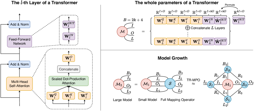
Figure 4: The full mapping of the Mango operator. The left sub-figure shows that the parameters of a Transformer layer are $\mathbf{W}^{Q},\mathbf{W}^{K},\mathbf{W}^{V},\mathbf{W}^{O}$, $\mathbf{W}^{IN}$ and $\mathbf{W}^{OUT}$. $I$ means an input dimension size. $O$ denotes an output dimension size. $L$ is the layer number. We concatenate all the parameters into a tensor $\bm{\mathcal{M}}$ and then consider a full mapping operator $\bm{\mathcal{S}}$ to transform this tensor. However, $\bm{\mathcal{S}}$ is huge, thereby, we use a multi-linear method TR-MPO to decompose it into four smaller tensors $\{\bm{\mathcal{S}}_{B},\bm{\mathcal{S}}_{I},\bm{\mathcal{S}}_{O},\bm{\mathcal{S}}_{L}\}$ form the Mango operator $\Phi_{\bm{\mathcal{S}}_{B},\bm{\mathcal{S}}_{I},\bm{\mathcal{S}}_{O},\bm{\mathcal{S}}_{L}}$.

3.2 Multi-linear Operator

The essential of model growth is to transfer the knowledge from the small model to the bigger counterpart. Prior study [5] finds that taking weights from the neighbor layer as initial parameters can further improve the convergence speed, which gives the insights that knowledge from other layers can help training as there are many similar attention maps among layer. Nevertheless, the fact is that this similarity exists all over the pretrained model as shown in Figure 2, which motivates us to consider the possibility of whether we can utilize the knowledge from all weights. Based on this consideration, we construct a mapping of the whole model. As the correlation is hard to formulate heuristically, we learn the mapping parameter to implicitly transfer the pretrained model.

Notation. Here, we give the notations for clearly formulating our method. A model with $L$ layers and a $D$ hidden size can be denoted as $\mathbf{M}(L,D)$. Following Section 3.1, parameters of $j$-th layer are a set $\bm{\theta}_{j}=\{\mathbf{W}_{j}^{Q}\in\mathbb{R}^{I\times O},\mathbf{W}_{j}^{K}\in\mathbb{R}^{I\times O},\mathbf{W}_{j}^{V}\in\mathbb{R}^{I\times O},\mathbf{W}_{j}^{O}\in\mathbb{R}^{I\times O},\mathbf{W}_{j}^{IN}\in\mathbb{R}^{I\times kO},\mathbf{W}_{j}^{OUT}\in\mathbb{R}^{kI\times O}\}$, $j\in[L]$, usually satisfying $I=O=D$. The weight of $\mathbf{M}(L,D)$ is $\bm{\theta}^{L,D}=\{\theta_{j}\}^{L}_{j=1}$. A growth operator with parameter $\bm{\mathcal{S}}$ is denoted as $\Phi_{\bm{\mathcal{S}}}$. A mapping from $\mathbf{M}(L_{1},D_{1})\rightarrow\mathbf{M}(L_{2},D_{2})$ can be denoted as $\bm{\theta}^{L_{2},D_{2}}=\Phi_{\bm{\mathcal{S}}}(\bm{\theta}^{L_{1},D_{1}})$. In the case of $L_{1}<L_{2}$, this mapping represents a growth mapping. After growing, $\bm{\theta}^{L_{2},D_{2}}$ will be used as initial weights for the target model.

Full Mapping Operator. To utilize all weights for knowledge transferring, we first concatenate weights across layers. As shown in Figure 4, we concatenate $j$-th layer to form a tensor of shape ${B\times I\times O}$ along with order $I$ and $O$ where $B=2k+4$. Then the final weight tensor $\bm{\mathcal{M}}\in\mathbb{R}^{B\times I\times O\times L}$ can be derived by combining the concatenated tensors of $L$ layers. Giving a small model $\bm{\mathcal{M}}_{1}\in\mathbb{R}^{B_{2}\times I_{1}\times O_{1}\times L_{1}}$, a big model $\bm{\mathcal{M}}_{2}\in\mathbb{R}^{B_{1}\times I_{2}\times O_{2}\times L_{2}}$, and a parameter $\bm{\mathcal{S}}\in\mathbb{R}^{B_{1}\times I_{1}\times O_{1}\times L_{1}\times B_{2}\times I_{2}\times O_{2}\times L_{2}}$ of a full mapping operator $\Phi_{\bm{\mathcal{S}}}$, we can transfer $\bm{\mathcal{M}}_{1}$ to $\bm{\mathcal{M}}_{2}$ as

$$(\bm{\mathcal{M}}_{2})_{b_{2},i_{2},o_{2},l_{2}}=\sum\limits_{b_{1},i_{1},o_{1},l_{1}}(\bm{\mathcal{M}}_{1})_{b_{1},i_{1},o_{1},l_{1}}\bm{\mathcal{S}}_{b_{1},i_{1},o_{1},l_{1},b_{2},i_{2},o_{2},l_{2}},$$ (5)

where $b_{1}$, $i_{1}$, $o_{1}$, $l_{1}$, $b_{2}$, $i_{2}$, $o_{2}$, and $l_{2}$ are entries of corresponding tensors.

Multi-linear Mapping Operator. Note that $\bm{\mathcal{S}}$ is extremely big, which makes it infeasible to display this mapping by applying a whole transformation tensor. Therefore, we propose a multi-linear operator named Mango which decomposes $\bm{\mathcal{S}}$ through a tensor ring matrix product operator (TR-MPO) in four small tensors $\{\bm{\mathcal{S}}_{B}\in\mathbb{R}^{R_{1}\times B_{1}\times B_{2}\times R_{2}},\bm{\mathcal{S}}_{O}\in\mathbb{R}^{R_{2}\times O_{1}\times O_{2}\times R_{3}},\bm{\mathcal{S}}_{L}\in\mathbb{R}^{R_{3}\times L_{1}\times L_{2}\times R_{4}},\bm{\mathcal{S}}_{I}\in\mathbb{R}^{R_{4}\times I_{1}\times I_{2}\times R_{1}}\}$. $R=\{R_{1},R_{2},R_{3},R_{4}\}$ is the rank of TR-MPO. Then, we can update $\Phi_{\bm{\mathcal{S}}}$ to $\Phi_{\bm{\mathcal{S}}_{B},\bm{\mathcal{S}}_{I},\bm{\mathcal{S}}_{O},\bm{\mathcal{S}}_{L}}$, and Eq. (5) can be reformulated with a multi-linear form as

$$(\bm{\mathcal{M}}_{2})_{b_{2},i_{2},o_{2},l_{2}} =\sum\limits_{b_{1},i_{1},o_{1},l_{1},r_{1},r_{2},r_{3},r_{4}}$$

$$(\bm{\mathcal{M}}_{1})_{b_{1},i_{1},o_{1},l_{1}}(\bm{\mathcal{S}}_{B})_{r_{1},b_{1},b_{2},r_{2}}(\bm{\mathcal{S}}_{O})_{r_{2},o_{1},o_{2},r_{3}}(\bm{\mathcal{S}}_{L})_{r_{3},l_{1},l_{2},r_{4}}(\bm{\mathcal{S}}_{I})_{r_{4},i_{1},i_{2},r_{1}}.$$ (6)

The total size of $\bm{\mathcal{S}}_{B}$, $\bm{\mathcal{S}}_{I}$, $\bm{\mathcal{S}}_{O}$, and $\bm{\mathcal{S}}_{L}$ is exponentially less than $\bm{\mathcal{S}}$, which makes Mango viable for practical implementation while maintaining the full correlation between the small and big models.

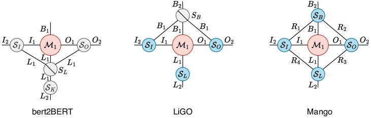
Figure 5: Growth processes with the tensor diagram. The circle with an oblique stroke means a super-diagonal tensor. The blue color means a trainable operator, while the gray color denotes an untrainable operator. The red color means the smaller model. Each tensor diagram means the growth process that growing $M_{1}$ to a bigger model through growth the operator $S_{\ast}$.

Training Target. After designing the multi-linear operators, we train these operators to obtain the function preserving $\bm{\mathcal{M}}_{2}$. The training target can be denoted as

$$\min\limits_{\bm{\mathcal{S}}_{B},\bm{\mathcal{S}}_{I},\bm{\mathcal{S}}_{O},\bm{\mathcal{S}}_{L}}\mathbb{E}_{\mathbf{X}\sim\mathcal{D}}\bm{\mathcal{L}}(\mathbf{X},\bm{\mathcal{M}}_{2}),~{}~{}\text{w.r.t}~{}~{}\bm{\mathcal{M}}_{2}=\Phi_{\bm{\mathcal{S}}_{B},\bm{\mathcal{S}}_{I},\bm{\mathcal{S}}_{O},\bm{\mathcal{S}}_{L}}(\bm{\mathcal{M}}_{1}),$$ (7)

where $\bm{\mathcal{L}}$ is a loss function, and $\mathcal{D}$ is a data distribution. By replacing the full space of $\bm{\mathcal{S}}$ with four small spaces, the spatial requirements of the training process are reduced exponentially.

Procedures of Applying Mango. The procedures of Mango can be divided into four steps: (i) concatenating weights $\theta^{L_{1},D_{1}}$ of a pretrained model $\mathbf{M}(L_{1},D_{1})$ to construct a tensor $\bm{\mathcal{M}}_{1}$; (ii) training the growth operator $\Phi_{\bm{\mathcal{S}}_{B},\bm{\mathcal{S}}_{I},\bm{\mathcal{S}}_{O},\bm{\mathcal{S}}_{L}}$ items of Eq. (7) in a few steps (e.g., 100) to make transferred models maintaining function; (iii) recovering weight tensor $\bm{\mathcal{M}}_{2}$ through the multi-linear operator $\Phi_{\bm{\mathcal{S}}_{B},\bm{\mathcal{S}}_{I},\bm{\mathcal{S}}_{O},\bm{\mathcal{S}}_{L}}$; (iv) splitting $\bm{\mathcal{M}}_{2}$ to the weight $\theta^{L_{2},D_{2}}$ of the target model $\mathbf{M}(L_{2},D_{2})$ as initialization to continue training.

Remark. Tensor decomposition is often used to compress neural networks. Actually, there are spaces for further reducing the operator size. However, we are not exploring the border of compression ratio, but the possibility of the learning ability of multi-linear operators and the influence on model growth. Therefore, we decompose the huge $\bm{\mathcal{S}}$ into four interpretable smaller tensors. $\bm{\mathcal{S}}_{B}$ means the interactions on the parameters in the same layer. $\bm{\mathcal{S}}_{I}$ and $\bm{\mathcal{S}}_{O}$ denote the transformations of input and output dimensions in one parameter, respectively. $\bm{\mathcal{S}}_{L}$ indicates the relationship among layers. $R$ means the low-rank level of $\bm{\mathcal{S}}$. Smaller $R$ means less correlation of these four tensors.

3.3 Comparison with Recent Advances

Basically, the goal of model growth is to widen and deepen the width and depth of the pretrained models, and operation on width and depth can be easy to implement. Therefore, most of the previous studies grow width and depth separately, although there may exist some correlation that may influence the training efficiency. In this part, we analyze the difference among methods of model growth with the help of the tensor diagrams.

We illustrate a comparison among bert2BERT, LiGO, and Mango in Figure 5. The red circle means a pretrained model, while the blue and gray circles denote trainable and untrainable operator parameters, respectively. The circle with an oblique stroke represents a super-diagonal tensor, where the diagonal elements are all 1. This super-diagonal tensor means that growth operators expand other modes along the mode of the super-diagonal tensor.

Table 1: The comparison among bert2BERT, LiGO and Mango. In a case of $\mathbf{M}(L_{1},D_{1})\rightarrow\mathbf{M}(L_{2},D_{2})$, there usually are $I_{1}=O_{1}=D_{1}$ and $I_{2}=O_{2}=D_{2}$. $R=\max(R_{1},R_{2},R_{3},R_{4})$.

Method	Reference	Operator Parameter	Trainability	Spatial Complexity
bert2BERT	Chen et al. [5]	$\bm{\mathcal{S}}_{I}$, $\bm{\mathcal{S}}_{O}$, $\bm{\mathcal{S}}_{K}$	✗	$2L_{1}D_{1}D_{2}+L_{1}L_{2}$
LiGO	Wang et al. [53]	$\bm{\mathcal{S}}_{I}$, $\bm{\mathcal{S}}_{O}$, $\bm{\mathcal{S}}_{L}$	✓	$2B_{1}D_{1}D_{2}+L_{1}L_{2}$
Mango	-	$\bm{\mathcal{S}}_{B}$, $\bm{\mathcal{S}}_{I}$, $\bm{\mathcal{S}}_{O}$, $\bm{\mathcal{S}}_{L}$	✓	$2RD_{1}D_{2}+R^{2}(B_{1}B_{2}+L_{1}L_{2})$

bert2BERT. As shown in Figure 5, the parameters in the growth operator of bert2BERT are all frozen, since they are designed by heuristic inspiration to preserve function. bert2BERT expands modes of $I_{1}$ and $O_{1}$ along with the mode of $L_{1}$, indicating that one weight is expanded without knowledge from any other weight. To further increase the training ability, bert2BERT applies $\bm{\mathcal{S}}_{K}$ to construct Advanced Knowledge Initialization (AKI) to utilize knowledge of other layers to help accelerate training.

LiGO. Different from bert2BERT, the LiGO operator can be trained. In addition, LiGO expands $I_{1}$ and $O_{1}$ along the mode of $B_{1}$. With $\bm{\mathcal{S}}_{L}$, LiGO can combine knowledge among layers. Operators of Net2Net and StackBERT grow with or depth separately, which can be regarded as a sub-solution to $\bm{\mathcal{S}}_{I}$, $\bm{\mathcal{S}}_{O}$, and $\bm{\mathcal{S}}_{L}$ of LiGO. However, one weight in LiGO will not leverage the knowledge of weights in the same layer. Therefore, LiGO only implements partial mapping like bert2BERT.

Mango. We employ Mango on each mode of the weight $\bm{\mathcal{M}}_{1}$. Mango can approach the full mapping tensor $\bm{\mathcal{S}}$ as a low-rank approximation with rank $R$, rather than partial mapping operators like LiGO and bert2BERT. Therefore, Mango can obtain $\bm{\mathcal{M}}_{2}$ to capture adequate knowledge from pretrained weights as formulated in Eq. 3.2. Moreover, the diagonal tensor in LiGO and contraction between a diagonal tensor and $\bm{\mathcal{S}}_{K}$ in bert2BERT are subsets of $\bm{\mathcal{S}}_{L}$ and $\bm{\mathcal{S}}_{B}$ in Mango. Therefore, Mango can be a generalization of bert2BERT and LiGO with more expressive power.

4 Experiment

In this section, we design a set of experiments to validate the proposed Mango. To begin with, we conduct an ablation study to analyze the influence of Mango on width and depth in Sec. 4.1. Then we conduct image classification with DeiT-B [46] on ImageNet to show the acceleration in computer vision task in Sec. 4.2. Later we conduct a pretraining experiment with BERT-Base [10] to demonstrate the effectiveness in natural language processing tasks in Sec. 4.3. At last, we also employ a pretraining experiment with GPT-Base [39] to show the wide adaption of Mango in Sec. 4.4.

Ratio of saving FLOPs.

We evaluate the training efficiency in terms of the ratio of saved floating-point operations (FLOPs). Let us assume that training a model from scratch to convergence on metric $\Psi$ (e.g., MLM loss or accuracy) necessitates $\xi_{Scratch}$ FLOPs. Then, for a method that reaches the same metric $\Psi$ with $\xi_{\ast}$ FLOPs, its FLOP saving ratio $r$ can be computed as

$$r=\frac{\xi_{Scratch}-\xi_{\ast}}{\xi_{Scratch}}.$$ (8)

4.1 Ablation Study

In this experiment, we explore the influence of Mango on growing width, depth and both of them in addition to rank setting. We use three tiny vision Transformers (ViTs) [11], i.e., DeiT-T-A, DeiT-T-B, and DeiT-T-C, for growing to DeiT-S [46] on ImageNet [9]. Structures of these DeiTs can be found in Table 4 of the Appendix. For ease of setting, we set all the ranks the same in the range of $\{1,4,7,10\}$. We train Mango operators for 100 steps, which only requires negligible time. We use Adam with learning rate 1e-3 and weight decay 1e-2 for 300 epoch optimization. The batch size is 1024.

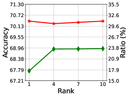
(a) Width: DeiT-T-A$\rightarrow$DeiT-S.

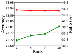
(b) Depth: DeiT-T-B$\rightarrow$DeiT-S.

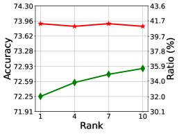
(c) Both: DeiT-T-C$\rightarrow$DeiT-S.

Figure 6: Influence from ranks on expanding width, depth, and both of them. The green curve means the accuracy of training operators for 100 steps. The red curve means the final acceleration ratio on training DeiT-S. Mango can achieve training acceleration in every case. Moreover, in each sub-graph, when the accuracy increases with a higher rank, the acceleration ratio keeps almost fixed.

Results are shown in Figure 6. Mango achieves acceleration of at most 31.0%, 46.0%, and 41.3% on expanding width, depth, and both of them, respectively, which shows Mango can fit various growth scenarios. Interestingly, these acceleration ratios are higher when the operator accuracies are better along the types of pretrained models, e.g., as DeiT-T-B at most achieves 73.81% accuracy which is higher than 72.89% of DeiT-T-A, DeiT-T-B derives higher acceleration ratio. This phenomenon suggests that when there are multiple pretrained models can be selected, the better accuracy for one pretrained model through Mango, the faster training speed can be obtained for the target models.

In each expanding case, the accuracies of operator training tend to increase with higher ranks. However, all the cases on the three pretrained models show that better accuracy will not lead to faster training with the same pretrained model. For example, in Figure 6(a), the operator with rank 10 has an accuracy that is 1.19% higher than the operator with rank 1. Nevertheless, the two ranks reach the same acceleration ratio. This result suggests that rank 1 is enough to use, and also enjoys the advantages of spatial and temporal complexities compared to bigger ranks. And we choose rank 1 for Mango to construct the later experiments.

4.2 Results on Large-Scale Vision Transformer

We conduct the experiment to show the training acceleration on large-scale vision Transformers. We train the Deit-B from Deit-S [46] on ImageNet. Structures of the two models are shown in Table 4 of the Appendix. Ranks of Mango are all set to 1 for complexity benefit without performance loss. The operators of Mango and Ligo are all trained within 100 steps. We use Adam as the optimizer with learning rate 1e-3 and weight decay 1e-2. The batch size is 1024. The training epoch is 300.

Results are shown in Figure 7(a). Mango saves 76% FLOPs from Scratch which converges to an accuracy of 80.45% in the end. Compared with schemes of training from Scratch (i.e., Srcatch and StackBERT), methods of training from a smaller model (i.e., Mango, bert2BERT, and LiGO) can attain 70% accuracy in a short time, even bert2BERT start in low accuracy. Compared with the recent SOTA models, Mango has surpassed bert2BERT for +12.0%, and LiGO for +20.7%. This experiment shows the ability of Mango to achieve significant improvement in training acceleration. To investigate the influence of Mango on transferring ability, we also conduct an experiment on downstream tasks, including CIFAR10 [26], CIFAR100 [26], Flowers [31], Cars [25], and ChestXRay8 [54]. Results are shown in Table 2. It is easy to see that Mango achieves similar results to the Scratch, which indicates Mango has not influenced the transferring ability.

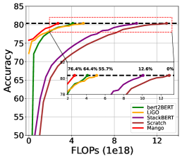
(a) DeiT-S$\rightarrow$DeiT-B.

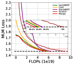
(b) BERT-Small$\rightarrow$BERT-Base.

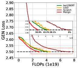
(c) GPT-Small$\rightarrow$GPT-Base.

Figure 7: Results of pretraining DeiT-B, BRET-Base and GPT-Base. Compared to baselines, Mango can achieve the highest savings in FLOPs with 76.4% for DeiT-B, 39.2% for BERT-Base, and 59.9% for GPT-Base from the Scratch model. We also illustrate the corresponding results on wall time in Figure 10 of the appendix.

Table 2: Results of transfer learning performance of DeiT-B. Mango can achieve similar performance to the Scratch model in downstream tasks while saving 76.4% FLOPs.

Method	FLOPs    ($\times$ 1e18)	Ratio    (Saving)	CIFAR10	CIFAR100	Flowers	Cars	ChestXRay8	Average
Training from Scratch
Scratch	12.9	-	99.03	90.22	97.27	91.89	55.66	86.82
StackBERT	11.3	12.6%	99.11	90.10	97.44	91.71	55.63	86.80
Training from the Pretrained Model: $\mathbf{M}(12,384)\rightarrow\mathbf{M}(12,768)$
bert2BERT	4.6	64.4%	98.99	90.47	97.51	91.88	55.34	86.84
LiGO	5.7	55.7%	99.11	90.52	97.18	91.82	55.45	86.82
Mango	3.0	76.4%	99.13	90.23	97.49	91.83	55.46	86.83

4.3 Pretraining on BERT

In this experiment, we conduct the validation to show the training acceleration on BERT [10, 61]. The dataset is the concatenation of English Wikipedia and Toronto Book Corpus [71]. We train the BERT-Base from BERT-Small. The training epoch is 40. The batch size is 768. We list the structures of the two models in Table 5 of the Appendix. The ranks of Mango are all 1. Mango and LiGO are both warmly trained for 100 steps. The optimizer is set to AdamW. The learning rate is 1e-4 and the weight decay is 1e-2.

We illustrate the training curves in Figure 7(b). The methods of training from BERT-Small (i.e., Mango, bert2BERT, and LiGO) can all surpass the progressive training StackBERT of acceleration ratio 29.5%. bert2BERT is over StackBERT by +6.1%. Mango achieves the highest acceleration of 39.2% FLOPs which is +3.6% more than bert2BERT. Loss of StackBERT steeply decreases within training for Stacking layers, which can also demonstrate the pretrained weights are helpful for training efficiency. We show the effectiveness of Mango on SQuAD and GLUE benchmark as in Table 3. Mango shows the same transferring ability with faster convergence, which indicates a promising use for practical training.

4.4 Pretraining on GPT

Table 3: Results of downstream tasks of BERT-Base on GLUE [48], SQuADv1.1 [40], and SQuADv2.0 [41] dataset. Mango can also achieve similar performance with the Scratch model while enjoying training efficiency.

Model	FLOPs ($\times$ 1e19)	Ratio (Saving)	SQuADv1.1 (F1)	SQuADv2.0 (F1)	SST-2 (Acc)	MNLI (Acc)	MRPC (Acc)	COLA (Mcc)	QNLI (Acc)	STS-B (Acc)	QQP (Acc)	GLUE Avg.	SQuAD Avg.
Training from Scratch
Scratch	8.9	-	89.21	77.90	92.18	84.19	87.55	56.35	91.50	89.16	90.25	84.45	83.56
StackBERT	6.3	29.5%	89.82	78.21	92.94	84.63	87.65	61.61	90.95	87.13	90.20	85.01	84.01
Training from the Pretrained Model: $\mathbf{M}(12,384)\rightarrow\mathbf{M}(12,768)$
bert2BERT	5.7	35.6%	90.02	78.99	92.89	84.92	86.91	60.32	91.81	88.11	90.72	85.10	84.50
LiGO	5.9	33.5%	90.09	78.34	92.75	84.99	87.44	61.10	91.33	87.94	90.42	85.14	84.22
Mango	5.4	39.2%	90.17	78.77	92.71	84.86	87.94	62.88	91.49	88.73	90.62	85.60	84.47

We also implement the experiment to show the training acceleration on GPT [39]. The dataset is the concatenation of English Wikipedia and Toronto Book Corpus [71]. We train the GPT-Base from GPT-Small. The structures of the two models are shown in Table 5 of the Appendix. The ranks of Mango are all 1. Mango and LiGO are trained for 100 steps. We use Adamw with learning rate 1e-4 and weight decay 1e-2. The batch size is 512. The training epoch is 35.

We compare the Scratch model, bert2BERT, LiGO, and Mango in Figure 7(c). We observe that the proposed Mango achieves a 59.9% acceleration ratio. While GPT is different from BERT in different structures, including layer normalization, mask method, and training strategy, Mango can always keep the highest performance. Although LiGO is lower than bert2BERT at the beginning, it converges slower and reaches 38.1% at last. By contrast, the Mango is almost at the lowest loss in the whole training process and achieves +16.7% more than bert2BERT and +21.8% more than LiGO, which shows a significant acceleration than the baselines.

5 Conclusion

Training Transformers can pose a significant demand on computational resources. Reusing pretrained models as an initialization strategy for the target model offers a promising approach to reducing resource costs and accelerating training. However, previous studies only mapped partial weights when growing models, which may fail to consider potential correlations in the whole model and result in inadequate growth mapping. Inspired by this observation, we propose to consider the interaction among all weights in the model to further improve acceleration ability. Specifically, we utilize a full mapping to comprehensively reuse the pretrained model, taking into account all correlations between model weights. As the full mapping tensor is huge and cannot be employed in practice, we propose to use Mango, a multi-linear operator, to reduce computation and space complexity. Experimental results demonstrate that Mango consistently achieves significant acceleration on various large-scale models (e.g., DeiT-B, BERT-Base, and GPT-Base). In the future, we hope that this method can contribute to green AI and significantly reduce the cost of training Transformers.

Limitation. While Mango significantly reduces training costs for large models, it still requires weights of a small pretrained model as the prior knowledge. Additionally, the Mango operator necessitates extra training for initializing. However, obtaining small model weights is relatively simple within the community, and given the substantial cost savings, the resources required for training the operator are minimal.

Societal Impact. The acceleration from Mango significantly impacts energy conservation and environmental protection, promoting the growth of Green AI, which boosts efficiency and reduces computational demand, minimizing energy usage and carbon emissions. Mango can also democratize AI, allowing broader access to technologies of pertaining models without the need for large resources, and promoting sustainable and accessible AI solutions that respect our environmental limits.

Appendix

Appendix A Additional Experiments and Details

A.1 Experiment Structures

We show DeiT structures in Table 4, and structures of BERT and GPT in Table 5.

Table 4: The structures of DeiT.

Config	DeiT-T-A	DeiT-T-B	DeiT-T-C	DeiT-S	DeiT-B
# layers	12	8	10	12	12
# hidden	192	384	320	384	768
# heads	3	6	5	6	12
input size	224	224	224	224	224
patch size	16	224	16	16	16

Table 5: The structures of BERT and GPT.

Config	BERT-Small	BERT-Base	BERT-Large	GPT-Small	GPT-Base
# layers	12	12	24	12	12
# hidden	512	768	1024	512	768
# heads	8	12	16	8	12
# vocab	30522	30522	30522	50257	50257
seq. length	512	512	512	1024	1024

A.2 Additional Experiment of Growing Swin-T to Swin-S

We also conduct an experiment to show the training acceleration on Swin-Transformers [29]. We train Swin-S from Swin-T with 128 batch size for 240 epochs. The training dataset is ImageNet. Ranks of Mango are all set to 1. The operators of Mango and Ligo are all trained within 100 steps. We use Adamw as the optimizer with a learning rate 1e-3 and weight decay 1e-8. The learning rate is reduced through a cosine scheme.

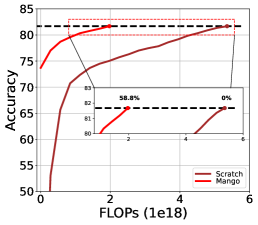
(a) FLOPs.

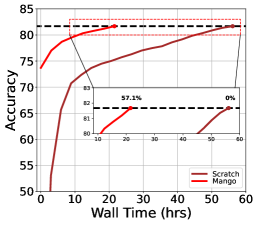
(b) Wall time.

Figure 8: Results on Swin-T$\rightarrow$Swin-S.

Results are shown in Figure 8. Mango saves 58.8% FLOPs and 57.1% wall time from Scratch which converges to an accuracy of 81.67%. Showing the effectiveness of Mango on Swin-Transformers, we demonstrate the potential of Mango to serve as a general-purpose growth operator.

A.3 Additional Experiment of Growing BERT-Base to BERT-Large

We also conduct an experiment to show the training acceleration on BERT-Large form BERT-Base with 512 batch size for 3 epochs. The structures of the two models are shown in Table 5 of the Appendix. Other settings follow Sec. 4.3.

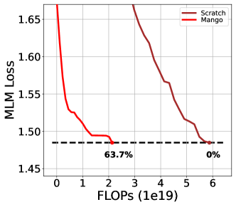
Figure 9: Results on BERT-Base$\rightarrow$BERT-Large.

We illustrate the training curves in Figure 9. Mango achieves 63.7% acceleration in an early training stage, indicating consistent acceleration to other experiments. This experiment shows that the proposed Mango can perform the same training efficiency even in a huge Transformer model.

Table 6: Detailed downstream results on the ImageNet.

Method	FLOPs ($\times$ 1e18)	Ratio (Saving)	CIFAR10	CIFAR100	Flowers	Cars	ChestXRay8	Average
Training from Scratch
Scratch	12.9	-	99.03 (0.08)	90.22 (0.27)	97.27 (0.17)	91.89 (0.53)	55.66 (0.23)	86.82 (0.26)
StackBERT	11.3	12.6%	99.11 (0.11)	90.10 (0.28)	97.44 (0.25)	91.71 (0.28)	55.63 (0.38)	86.80 (0.26)
Training from the Pretrained Model: $\mathbf{M}(12,384)\rightarrow\mathbf{M}(12,768)$
bert2BERT	4.6	64.4%	98.99 (0.04)	90.47 (0.19)	97.51 (0.07)	91.88 (0.47)	55.34 (0.22)	86.84 (0.20)
LiGO	5.7	55.7%	99.11 (0.08)	90.52 (0.33)	97.18 (0.27)	91.82 (0.36)	55.45 (0.26)	86.82 (0.26)
Mango	3.0	76.4%	99.13 (0.06)	90.23 (0.24)	97.49 (0.15)	91.83 (0.34)	55.46 (0.36)	86.83 (0.23)

Table 7: Detailed downstream results on the GLUE benchmark.

Model	FLOPs ($\times$ 1e19)	Ratio (Saving)	SST-2 (Acc)	MNLI (Acc)	MRPC (Acc)	COLA (Mcc)	QNLI (Acc)	STS-B (Acc)	QQP (Acc)	GLUE Avg.
Training from Scratch
Scratch	8.9	-	92.18(0.09)	84.19(0.17)	87.55(0.29)	56.35(1.93)	91.50(0.09)	89.16(0.28)	90.25(0.13)	84.45(0.42)
StackBERT	6.3	29.5%	92.94(0.06)	84.63(0.19)	87.65(0.20)	61.61(3.58)	90.95(0.10)	87.13(0.60)	90.20(0.15)	85.01(0.70)
Training from the Pretrained Model: $\mathbf{M}(12,384)\rightarrow\mathbf{M}(12,768)$
bert2BERT	5.7	35.6%	92.89(0.65)	84.92(0.19)	86.91(0.70)	60.32(2.16)	91.81(0.34)	88.11(0.57)	90.72(0.13)	85.10(0.68)
LiGO	5.9	33.5%	92.75(0.37)	84.99(0.12)	87.44(1.13)	61.10(1.03)	91.33(0.23)	87.94(0.44)	90.42(0.13)	85.14(0.49)
Mango	5.4	39.2%	92.71(0.20)	84.86(0.22)	87.94(1.11)	62.88(0.86)	91.49(0.12)	88.73(0.35)	90.62(0.20)	85.60(0.44)

Table 8: Detailed downstream results on the SQuADv1.1 and SQuADv2.0 datasets.

Model	FLOPs ($\times$ 1e19)	Ratio (Saving)	SQuADv1.1		SQuADv2.0		SQuAD Avg.
			F1	EM	F1	EM	F1	EM
Training from Scratch
Scratch	8.9	-	89.21(0.16)	82.07(0.30)	77.90(0.36)	74.85(0.40)	83.56(0.26)	78.46(0.35)
StackBERT	6.3	29.5%	89.82(0.14)	82.89(0.16)	78.21(0.38)	75.18(0.44)	84.01(0.26)	79.03(0.30)
Training from the Pretrained Model: $\mathbf{M}(12,384)\rightarrow\mathbf{M}(12,768)$
bert2BERT	5.7	35.6%	90.02(0.36)	83.24(0.52)	78.99(0.31)	75.98(0.35)	84.50(0.34)	79.61(0.43)
LiGO	5.9	33.5%	90.09(0.31)	82.77(0.19)	78.34(0.24)	75.31(0.24)	84.22(0.28)	79.04(0.21)
Mango	5.4	39.2%	90.17(0.27)	83.29(0.33)	78.77(0.18)	75.71(0.14)	84.47(0.22)	79.50(0.24)

A.4 Details of Training Mango

In experiments of DeiTs, we train Mango operators with Adam optimizer for 100 steps on ImageNet. The learning rate is 1e-4. Minibatch is 1536.

In experiments of BERT and GPT models, we train Mango operators with Adamw optimizer for 100 steps on the concatenation of English Wikipedia and Toronto Book Corpus. The learning rate is 1e-5. Minibatch is 512.

A.5 Details of Downstream Tasks

In downstream tasks of DeiTs, we use Adam with a learning rate chosen from {8e-5, 1e-4}. The batch size is 256, and we run up to 100 epochs. We run each experiment three times for calculating mean and standard derivation. Detailed results are shown in Table 8.

In downstream tasks of BERT, we set the batch size to 32 and use Adam with the learning rate from {5e-6, 1e-5, 2e-5, 3e-5} and epochs from {4, 5, 10} for the GLUE tasks fine-tuning. For the SQuAD fine-tuning, we set the batch size to 16 and the learning rate to 3e-5, and train for 4 epochs. All results are the average of 5 runs on the dev set. Detailed results are shown in Table 8 and Table 8.

A.6 Wall Time of Experiments

We illustrate the acceleration of training DeiT-B, BERT-Base and GPT-Base in terms of wall time in Figure 10, which corresponds to Figure 7.

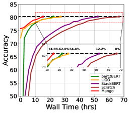
(a) DeiT-S$\rightarrow$DeiT-B.

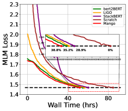
(b) BERT-Small$\rightarrow$BERT-Base.

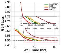
(c) GPT-Small$\rightarrow$GPT-Base.

Figure 10: Results of pretraining DeiT-B, BRET-Base and GPT-Base on the wall time.

References

- Bachlechner et al. [2021] Thomas Bachlechner, Bodhisattwa Prasad Majumder, Huanru Henry Mao, Gary Cottrell, and Julian J. McAuley. Rezero is all you need: fast convergence at large depth. In UAI, volume 161 of Proceedings of Machine Learning Research, pages 1352–1361. AUAI Press, 2021.
- Bolya et al. [2022] Daniel Bolya, Cheng-Yang Fu, Xiaoliang Dai, Peizhao Zhang, Christoph Feichtenhofer, and Judy Hoffman. Token merging: Your vit but faster. CoRR, abs/2210.09461, 2022.
- Brown et al. [2020] Tom B. Brown, Benjamin Mann, Nick Ryder, Melanie Subbiah, Jared Kaplan, Prafulla Dhariwal, Arvind Neelakantan, Pranav Shyam, Girish Sastry, Amanda Askell, Sandhini Agarwal, Ariel Herbert-Voss, Gretchen Krueger, Tom Henighan, Rewon Child, Aditya Ramesh, Daniel M. Ziegler, Jeffrey Wu, Clemens Winter, Christopher Hesse, Mark Chen, Eric Sigler, Mateusz Litwin, Scott Gray, Benjamin Chess, Jack Clark, Christopher Berner, Sam McCandlish, Alec Radford, Ilya Sutskever, and Dario Amodei. Language models are few-shot learners. In NeurIPS, 2020.
- Cao et al. [2021] Hu Cao, Yueyue Wang, Joy Chen, Dongsheng Jiang, Xiaopeng Zhang, Qi Tian, and Manning Wang. Swin-unet: Unet-like pure transformer for medical image segmentation. CoRR, abs/2105.05537, 2021.
- Chen et al. [2022a] Cheng Chen, Yichun Yin, Lifeng Shang, Xin Jiang, Yujia Qin, Fengyu Wang, Zhi Wang, Xiao Chen, Zhiyuan Liu, and Qun Liu. bert2bert: Towards reusable pretrained language models. In ACL (1), pages 2134–2148. Association for Computational Linguistics, 2022a.
- Chen et al. [2022b] Richard J. Chen, Chengkuan Chen, Yicong Li, Tiffany Y. Chen, Andrew D. Trister, Rahul G. Krishnan, and Faisal Mahmood. Scaling vision transformers to gigapixel images via hierarchical self-supervised learning. In CVPR, pages 16123–16134. IEEE, 2022b.
- Chen et al. [2016] Tianqi Chen, Ian J. Goodfellow, and Jonathon Shlens. Net2net: Accelerating learning via knowledge transfer. In ICLR, 2016.
- De and Smith [2020] Soham De and Samuel L. Smith. Batch normalization biases residual blocks towards the identity function in deep networks. In NeurIPS, 2020.
- Deng et al. [2009] Jia Deng, Wei Dong, Richard Socher, Li-Jia Li, Kai Li, and Li Fei-Fei. Imagenet: A large-scale hierarchical image database. In CVPR, pages 248–255. IEEE Computer Society, 2009.
- Devlin et al. [2019] Jacob Devlin, Ming-Wei Chang, Kenton Lee, and Kristina Toutanova. BERT: pre-training of deep bidirectional transformers for language understanding. In NAACL-HLT (1), pages 4171–4186. Association for Computational Linguistics, 2019.
- Dosovitskiy et al. [2021] Alexey Dosovitskiy, Lucas Beyer, Alexander Kolesnikov, Dirk Weissenborn, Xiaohua Zhai, Thomas Unterthiner, Mostafa Dehghani, Matthias Minderer, Georg Heigold, Sylvain Gelly, Jakob Uszkoreit, and Neil Houlsby. An image is worth 16x16 words: Transformers for image recognition at scale. In ICLR. OpenReview.net, 2021.
- Glorot and Bengio [2010] Xavier Glorot and Yoshua Bengio. Understanding the difficulty of training deep feedforward neural networks. In AISTATS, volume 9 of JMLR Proceedings, pages 249–256. JMLR.org, 2010.
- Gong et al. [2019] Linyuan Gong, Di He, Zhuohan Li, Tao Qin, Liwei Wang, and Tie-Yan Liu. Efficient training of BERT by progressively stacking. In ICML, volume 97 of Proceedings of Machine Learning Research, pages 2337–2346. PMLR, 2019.
- Gu et al. [2021] Xiaotao Gu, Liyuan Liu, Hongkun Yu, Jing Li, Chen Chen, and Jiawei Han. On the transformer growth for progressive BERT training. In NAACL-HLT, pages 5174–5180. Association for Computational Linguistics, 2021.
- Hardt and Ma [2017] Moritz Hardt and Tengyu Ma. Identity matters in deep learning. In ICLR (Poster). OpenReview.net, 2017.
- He et al. [2015] Kaiming He, Xiangyu Zhang, Shaoqing Ren, and Jian Sun. Delving deep into rectifiers: Surpassing human-level performance on imagenet classification. In ICCV, pages 1026–1034. IEEE Computer Society, 2015.
- Hu et al. [2022] Edward J. Hu, Yelong Shen, Phillip Wallis, Zeyuan Allen-Zhu, Yuanzhi Li, Shean Wang, Lu Wang, and Weizhu Chen. Lora: Low-rank adaptation of large language models. In ICLR. OpenReview.net, 2022.
- Hyeon-Woo et al. [2022] Nam Hyeon-Woo, Moon Ye-Bin, and Tae-Hyun Oh. Fedpara: Low-rank hadamard product for communication-efficient federated learning. In ICLR. OpenReview.net, 2022.
- Idelbayev and Carreira-Perpiñán [2020] Yerlan Idelbayev and Miguel Á. Carreira-Perpiñán. Low-rank compression of neural nets: Learning the rank of each layer. In CVPR, pages 8046–8056. Computer Vision Foundation / IEEE, 2020.
- Jiang et al. [2021] Yifan Jiang, Shiyu Chang, and Zhangyang Wang. Transgan: Two pure transformers can make one strong gan, and that can scale up. In NeurIPS, pages 14745–14758, 2021.
- Kamalakara et al. [2022] Siddhartha Rao Kamalakara, Acyr Locatelli, Bharat Venkitesh, Jimmy Ba, Yarin Gal, and Aidan N. Gomez. Exploring low rank training of deep neural networks. CoRR, abs/2209.13569, 2022.
- Kaplan et al. [2020] Jared Kaplan, Sam McCandlish, Tom Henighan, Tom B. Brown, Benjamin Chess, Rewon Child, Scott Gray, Alec Radford, Jeffrey Wu, and Dario Amodei. Scaling laws for neural language models. CoRR, abs/2001.08361, 2020.
- Kingma and Ba [2015] Diederik P. Kingma and Jimmy Ba. Adam: A method for stochastic optimization. In ICLR (Poster), 2015.
- Kossaifi et al. [2019] Jean Kossaifi, Adrian Bulat, Georgios Tzimiropoulos, and Maja Pantic. T-net: Parametrizing fully convolutional nets with a single high-order tensor. In CVPR, pages 7822–7831. Computer Vision Foundation / IEEE, 2019.
- Krause et al. [2013] Jonathan Krause, Michael Stark, Jia Deng, and Li Fei-Fei. 3d object representations for fine-grained categorization. In ICCV Workshops, pages 554–561. IEEE Computer Society, 2013.
- Krizhevsky et al. [2009] Alex Krizhevsky, Geoffrey Hinton, et al. Learning multiple layers of features from tiny images. 2009.
- Li et al. [2022] Changlin Li, Bohan Zhuang, Guangrun Wang, Xiaodan Liang, Xiaojun Chang, and Yi Yang. Automated progressive learning for efficient training of vision transformers. In CVPR, pages 12476–12486. IEEE, 2022.
- Li et al. [2021] Nannan Li, Yu Pan, Yaran Chen, Zixiang Ding, Dongbin Zhao, and Zenglin Xu. Heuristic rank selection with progressively searching tensor ring network. Complex & Intelligent Systems, pages 1–15, 2021.
- Liu et al. [2021] Ze Liu, Yutong Lin, Yue Cao, Han Hu, Yixuan Wei, Zheng Zhang, Stephen Lin, and Baining Guo. Swin transformer: Hierarchical vision transformer using shifted windows. In Proceedings of the IEEE/CVF international conference on computer vision, pages 10012–10022, 2021.
- Ma et al. [2019] Xindian Ma, Peng Zhang, Shuai Zhang, Nan Duan, Yuexian Hou, Ming Zhou, and Dawei Song. A tensorized transformer for language modeling. In NeurIPS, pages 2229–2239, 2019.
- Nilsback and Zisserman [2008] Maria-Elena Nilsback and Andrew Zisserman. Automated flower classification over a large number of classes. In ICVGIP, pages 722–729. IEEE Computer Society, 2008.
- Pan and Yang [2010] Sinno Jialin Pan and Qiang Yang. A survey on transfer learning. IEEE Trans. Knowl. Data Eng., 22(10):1345–1359, 2010.
- Pan et al. [2019] Yu Pan, Jing Xu, Maolin Wang, Jinmian Ye, Fei Wang, Kun Bai, and Zenglin Xu. Compressing recurrent neural networks with tensor ring for action recognition. In AAAI, pages 4683–4690. AAAI Press, 2019.
- Pan et al. [2022a] Yu Pan, Zeyong Su, Ao Liu, Jingquan Wang, Nannan Li, and Zenglin Xu. A unified weight initialization paradigm for tensorial convolutional neural networks. In International Conference on Machine Learning, ICML 2022, 17-23 July 2022, Baltimore, Maryland, USA, volume 162 of Proceedings of Machine Learning Research, pages 17238–17257. PMLR, 2022a.
- Pan et al. [2022b] Yu Pan, Maolin Wang, and Zenglin Xu. Tednet: A pytorch toolkit for tensor decomposition networks. Neurocomputing, 469:234–238, 2022b.
- Pan et al. [2022c] Yu Pan, Zekai Wu, Chaozheng Wang, Qifan Wang, Min Zhang, and Zenglin Xu. Identical initialization: A universal approach to fast and stable training of neural networks. Openreview.net, 2022c.
- Pirvu et al. [2010] Bogdan Pirvu, Valentin Murg, J Ignacio Cirac, and Frank Verstraete. Matrix product operator representations. New Journal of Physics, 12(2):025012, 2010.
- Qin et al. [2022] Yujia Qin, Yankai Lin, Jing Yi, Jiajie Zhang, Xu Han, Zhengyan Zhang, Yusheng Su, Zhiyuan Liu, Peng Li, Maosong Sun, and Jie Zhou. Knowledge inheritance for pre-trained language models. In NAACL-HLT, pages 3921–3937. Association for Computational Linguistics, 2022.
- Radford et al. [2019] Alec Radford, Jeffrey Wu, Rewon Child, David Luan, Dario Amodei, Ilya Sutskever, et al. Language models are unsupervised multitask learners. OpenAI blog, 1(8):9, 2019.
- Rajpurkar et al. [2016] Pranav Rajpurkar, Jian Zhang, Konstantin Lopyrev, and Percy Liang. Squad: 100, 000+ questions for machine comprehension of text. In EMNLP, pages 2383–2392. The Association for Computational Linguistics, 2016.
- Rajpurkar et al. [2018] Pranav Rajpurkar, Robin Jia, and Percy Liang. Know what you don’t know: Unanswerable questions for squad. In ACL (2), pages 784–789. Association for Computational Linguistics, 2018.
- Rosenfeld et al. [2020] Jonathan S. Rosenfeld, Amir Rosenfeld, Yonatan Belinkov, and Nir Shavit. A constructive prediction of the generalization error across scales. In ICLR. OpenReview.net, 2020.
- Schwartz et al. [2019] Roy Schwartz, Jesse Dodge, Noah A. Smith, and Oren Etzioni. Green AI. CoRR, abs/1907.10597, 2019.
- Shen et al. [2022] Sheng Shen, Pete Walsh, Kurt Keutzer, Jesse Dodge, Matthew E. Peters, and Iz Beltagy. Staged training for transformer language models. In ICML, volume 162 of Proceedings of Machine Learning Research, pages 19893–19908. PMLR, 2022.
- Shoeybi et al. [2019] Mohammad Shoeybi, Mostofa Patwary, Raul Puri, Patrick LeGresley, Jared Casper, and Bryan Catanzaro. Megatron-lm: Training multi-billion parameter language models using model parallelism. CoRR, abs/1909.08053, 2019.
- Touvron et al. [2021] Hugo Touvron, Matthieu Cord, Matthijs Douze, Francisco Massa, Alexandre Sablayrolles, and Hervé Jégou. Training data-efficient image transformers & distillation through attention. In ICML, volume 139 of Proceedings of Machine Learning Research, pages 10347–10357. PMLR, 2021.
- Vaswani et al. [2017] Ashish Vaswani, Noam Shazeer, Niki Parmar, Jakob Uszkoreit, Llion Jones, Aidan N. Gomez, Lukasz Kaiser, and Illia Polosukhin. Attention is all you need. In NIPS, pages 5998–6008, 2017.
- Wang et al. [2019a] Alex Wang, Amanpreet Singh, Julian Michael, Felix Hill, Omer Levy, and Samuel R. Bowman. GLUE: A multi-task benchmark and analysis platform for natural language understanding. In ICLR (Poster). OpenReview.net, 2019a.
- Wang et al. [2019b] Dilin Wang, Meng Li, Lemeng Wu, Vikas Chandra, and Qiang Liu. Energy-aware neural architecture optimization with fast splitting steepest descent. CoRR, abs/1910.03103, 2019b.
- Wang et al. [2018] Linnan Wang, Jinmian Ye, Yiyang Zhao, Wei Wu, Ang Li, Shuaiwen Leon Song, Zenglin Xu, and Tim Kraska. Superneurons: dynamic GPU memory management for training deep neural networks. In Proceedings of the 23rd ACM SIGPLAN Symposium on Principles and Practice of Parallel Programming, PPoPP 2018, Vienna, Austria, February 24-28, 2018, pages 41–53. ACM, 2018.
- Wang et al. [2019c] Maolin Wang, Chenbin Zhang, Yu Pan, Jing Xu, and Zenglin Xu. Tensor ring restricted boltzmann machines. In International Joint Conference on Neural Networks, IJCNN 2019 Budapest, Hungary, July 14-19, 2019, pages 1–8. IEEE, 2019c.
- Wang et al. [2023a] Maolin Wang, Yu Pan, Zenglin Xu, Xiangli Yang, Guangxi Li, and Andrzej Cichocki. Tensor networks meet neural networks: A survey and future perspectives. CoRR, abs/2302.09019, 2023a.
- Wang et al. [2023b] Peihao Wang, Rameswar Panda, Lucas Torroba Hennigen, Philip Greengard, Leonid Karlinsky, Rogerio Feris, David Daniel Cox, Zhangyang Wang, and Yoon Kim. Learning to grow pretrained models for efficient transformer training. In ICLR. OpenReview.net, 2023b.
- Wang et al. [2017] Xiaosong Wang, Yifan Peng, Le Lu, Zhiyong Lu, Mohammadhadi Bagheri, and Ronald M. Summers. Chestx-ray8: Hospital-scale chest x-ray database and benchmarks on weakly-supervised classification and localization of common thorax diseases. In CVPR, pages 3462–3471. IEEE Computer Society, 2017.
- Wang et al. [2022] Yulin Wang, Yang Yue, Rui Lu, Tianjiao Liu, Zhao Zhong, Shiji Song, and Gao Huang. Efficienttrain: Exploring generalized curriculum learning for training visual backbones. CoRR, abs/2211.09703, 2022.
- Wu et al. [2019] Lemeng Wu, Dilin Wang, and Qiang Liu. Splitting steepest descent for growing neural architectures. In NeurIPS, pages 10655–10665, 2019.
- Wu et al. [2020a] Lemeng Wu, Bo Liu, Peter Stone, and Qiang Liu. Firefly neural architecture descent: a general approach for growing neural networks. In NeurIPS, 2020a.
- Wu et al. [2020b] Lemeng Wu, Mao Ye, Qi Lei, Jason D. Lee, and Qiang Liu. Steepest descent neural architecture optimization: Escaping local optimum with signed neural splitting. CoRR, abs/2003.10392, 2020b.
- Wu et al. [2021] Qiyu Wu, Chen Xing, Yatao Li, Guolin Ke, Di He, and Tie-Yan Liu. Taking notes on the fly helps language pre-training. In ICLR. OpenReview.net, 2021.
- Xia et al. [2023] Zhuofan Xia, Xuran Pan, Xuan Jin, Yuan He, Hui Xue, Shiji Song, and Gao Huang. Budgeted training for vision transformer. In ICLR. OpenReview.net, 2023.
- Xiong et al. [2022] Jing Xiong, Chengming Li, Min Yang, Xiping Hu, and Bin Hu. Expression syntax information bottleneck for math word problems. In SIGIR, pages 2166–2171. ACM, 2022.
- Xiong et al. [2023] Jiong Xiong, Zixuan Li, Chuanyang Zheng, Zhijiang Guo, Yichun Yin, Enze Xie, Zhicheng Yang, Qingxing Cao, Haiming Wang, Xiongwei Han, Jing Tang, Chengming Li, and Xiaodan Liang. Dq-lore: Dual queries with low rank approximation re-ranking for in-context learning. CoRR, abs/2310.02954, 2023.
- Yang et al. [2020] Cheng Yang, Shengnan Wang, Chao Yang, Yuechuan Li, Ru He, and Jingqiao Zhang. Progressively stacking 2.0: A multi-stage layerwise training method for BERT training speedup. CoRR, abs/2011.13635, 2020.
- Ye et al. [2020] Jinmian Ye, Guangxi Li, Di Chen, Haiqin Yang, Shandian Zhe, and Zenglin Xu. Block-term tensor neural networks. Neural Networks, 130:11–21, 2020.
- Yin et al. [2021] Miao Yin, Yang Sui, Siyu Liao, and Bo Yuan. Towards efficient tensor decomposition-based DNN model compression with optimization framework. In CVPR, pages 10674–10683. Computer Vision Foundation / IEEE, 2021.
- You et al. [2020] Yang You, Jing Li, Sashank J. Reddi, Jonathan Hseu, Sanjiv Kumar, Srinadh Bhojanapalli, Xiaodan Song, James Demmel, Kurt Keutzer, and Cho-Jui Hsieh. Large batch optimization for deep learning: Training BERT in 76 minutes. In ICLR. OpenReview.net, 2020.
- Zhang et al. [2019] Hongyi Zhang, Yann N. Dauphin, and Tengyu Ma. Fixup initialization: Residual learning without normalization. In ICLR (Poster). OpenReview.net, 2019.
- Zhang and He [2020] Minjia Zhang and Yuxiong He. Accelerating training of transformer-based language models with progressive layer dropping. In NeurIPS, 2020.
- Zhang et al. [2023] Zhuo Zhang, Yuanhang Yang, Yong Dai, Qifan Wang, Yue Yu, Lizhen Qu, and Zenglin Xu. Fedpetuning: When federated learning meets the parameter-efficient tuning methods of pre-trained language models. In Findings of the Association for Computational Linguistics: ACL 2023, Toronto, Canada, July 9-14, 2023, pages 9963–9977. Association for Computational Linguistics, 2023.
- Zhao et al. [2021] Jiawei Zhao, Florian Schäfer, and Anima Anandkumar. Zero initialization: Initializing residual networks with only zeros and ones. CoRR, abs/2110.12661, 2021.
- Zhu et al. [2015] Yukun Zhu, Ryan Kiros, Richard S. Zemel, Ruslan Salakhutdinov, Raquel Urtasun, Antonio Torralba, and Sanja Fidler. Aligning books and movies: Towards story-like visual explanations by watching movies and reading books. In ICCV, pages 19–27. IEEE Computer Society, 2015.