Robust Collaborative Filtering to Popularity Distribution Shift

Abstract.

In leading collaborative filtering (CF) models, representations of users and items are prone to learn popularity bias in the training data as shortcuts. The popularity shortcut tricks are good for in-distribution (ID) performance but poorly generalized to out-of-distribution (OOD) data, i.e., when popularity distribution of test data shifts w.r.t. the training one. To close the gap, debiasing strategies try to assess the shortcut degrees and mitigate them from the representations. However, there exist two deficiencies: (1) when measuring the shortcut degrees, most strategies only use statistical metrics on a single aspect (i.e., item frequency on item and user frequency on user aspect), failing to accommodate the compositional degree of a user-item pair; (2) when mitigating shortcuts, many strategies assume that the test distribution is known in advance. This results in low-quality debiased representations. Worse still, these strategies achieve OOD generalizability with a sacrifice on ID performance.

In this work, we present a simple yet effective debiasing strategy, PopGo, which quantifies and reduces the interaction-wise popularity shortcut without any assumptions on the test data. It first learns a shortcut model, which yields a shortcut degree of a user-item pair based on their popularity representations. Then, it trains the CF model by adjusting the predictions with the interaction-wise shortcut degrees. By taking both causal- and information-theoretical looks at PopGo, we can justify why it encourages the CF model to capture the critical popularity-agnostic features while leaving the spurious popularity-relevant patterns out. We use PopGo to debias two high-performing CF models (MF (Koren, 2008), LightGCN (He et al., 2020)) on four benchmark datasets. On both ID and OOD test sets, PopGo achieves significant gains over the state-of-the-art debiasing strategies (e.g., DICE (Zheng et al., 2021), MACR (Wei et al., 2021)). Codes and datasets are available at https://github.com/anzhang314/PopGo.

1. Introduction

Leading collaborative filtering (CF) models (Koren, 2008; Rendle et al., 2012; Liang et al., 2018; He et al., 2020) follow a paradigm of supervised learning, which takes historical interactions among users and items as the training data, learns the representations of users and items, and consequently predicts future interactions. Clearly, representation learning is of critical importance to delineate user preference. However, the representations are susceptible to learning popularity bias in the training data as shortcuts. Typically, the popularity shortcut is the superficial correlations between popularity and user preference on a particular dataset (Jannach et al., 2015; Cañamares and Castells, 2018; Bellogín et al., 2017; Abdollahpouri et al., 2019; Park and Tuzhilin, 2008; Zhu et al., 2021), but are not helpful in general. When the test data follows the same distribution as the training data (i.e., in-distribution (ID)), it is much easier to reach a high recommendation accuracy by leveraging the popularity shortcut (Ji et al., 2020), instead of probing the actual preference of users. However, the representations that have achieved strong ID performance by utilizing shortcuts in the training dataset will generalize poorly when the shortcut is absent in the test set (i.e., out-of-distribution (OOD)). Specifically, by “OOD” w.r.t. popularity shortcut, we mean that the popularity distribution shifts between the training and test data. Considering the Tencent dataset (Yuan et al., 2020) as an example, we split it into the training, validation, ID test, and OOD test data, and then illustrate their popularity distributions in Figure 1(a). Clearly, the popularity distribution of the training data is similar to that of the ID test data, but significantly different from that of the OOD test data. Such a divergence leads to a performance drop of CF models (e.g., MF (Koren, 2008) and LightGCN (He et al., 2020)), as Figure 1(b) shows where these models perform well w.r.t. NDCG@20 on the ID test set, while generalizing poorly w.r.t. NDCG@20 on the OOD test set.

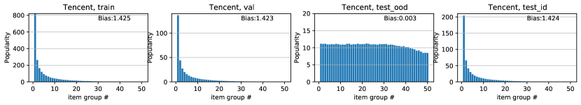
(a) Distribution shift w.r.t. item popularity.

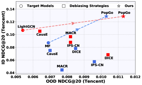
(b) Debiasing performance on Tencent.

Figure 1. (a) Popularity distribution of the training, validation, OOD testing, and ID testing sets for the Tencent dataset (Yuan et al., 2020). (b) Performance of debiasing strategies on the Tencent dataset, in both ID and OOD test evaluations. For strategies in blue and red, the target CF models being debiased are MF and LightGCN, respectively.

The crucial problem on the generalization of CF models motivates the task of debiasing, which aims to alleviate the popularity bias and close the gap between ID and OOD performance. The current in-processing debiasing strategies can be roughly categorized into five types: (1) Inverse Propensity Scoring (IPS) (Schnabel et al., 2016; Saito et al., 2020; Liang et al., 2016; Gruson et al., 2019; Joachims et al., 2018; Chen et al., 2021; Wang et al., 2019a), which views item popularity as the proxy of propensity score and exploits its inverse to reweight the loss of each user-item pair; (2) Domain adaption (Bonner and Vasile, 2018; Liu et al., 2020; Chen et al., 2020b), which uses a small amount of unbiased data as the target domain to guide the model training on biased source data; (3) Causal effect estimation (Zheng et al., 2021; Wei et al., 2021; Wang et al., 2021; Zhang et al., 2021b; Xu et al., 2021; Gupta et al., 2021; Liu et al., 2020), which specifies the role of popularity bias in causal graphs and mitigates its effect on the prediction. (4) Regularization-based framework (Abdollahpouri et al., 2017; Boratto et al., 2021; Zhu et al., 2021), which explores the use of regularization for controlling the trade-off between recommendation accuracy and coverage. (5) Generalized methods (Zhang et al., 2023a, 2022, b; Chen et al., 2022; Wen et al., 2022; Wang et al., 2022b; He et al., 2022; Wang et al., 2022a) learn invariant representations against popularity bias in order to achieve stability and generalization ability.

Regardless of diverse ideas, we can systematize these strategies as a standard paradigm of debiasing, which quantifies the degree of popularity shortcuts and removes them from the CF representations. However, there exist two deficiencies:

• When measuring the shortcut degrees, most strategies (Schnabel et al., 2016; Joachims et al., 2018; Zheng et al., 2021; Wei et al., 2021) only adopt statistical metrics on a single aspect (i.e., item/user frequency on item/user aspect), and fail to accommodate the compositional degree of a user-item pair. For example, the IPS family (Schnabel et al., 2016; Joachims et al., 2018) solely considers item frequency as the shortcut degree to reweight the user-item pairs, while CausE (Bonner and Vasile, 2018) partitions user-item pairs into biased and unbiased groups based only on item frequency. As a result, for different users, their distinct interactions with the same item are assigned with an identical shortcut degree, which fails to indicate the interaction-dependent shortcut. Hence, how to accurately identify the popularity shortcut is crucial to prevent CF models from making use of them.

• When mitigating the shortcut, many strategies (Zheng et al., 2021; Bonner and Vasile, 2018; Liu et al., 2020; Chen et al., 2020b) predetermine that the test distribution is known in advance to guide the debiasing. For example, CausE (Bonner and Vasile, 2018) involves a part of unbiased data which conforms to the test distribution during training, while MACR (Wei et al., 2021) needs the test distribution to adjust the key hyperparameters. However, such assumptions are usually infeasible for real-world or wild settings.

These limitations result in low-quality debiased representations, which hardly distinguish popularity-agnostic information from popularity shortcuts. Worse still, as Figure 1(b) shows, these strategies achieve higher OOD but lower ID performance, as compared with the non-debiasing CF models. We hence argue that the OOD improvements may result from the ID sacrifices, but not from the improved generalization ability.

In this work, we aim to truly improve the generalization by reducing popularity shortcuts and pursuing high-quality debiased representations, instead of finding a better trade-off between ID and OOD performance. Towards this end, we propose a simple yet effective strategy, PopGo, which quantifies the interaction-wise popularity shortcut without any assumptions on the test data. Before debiasing the target CF model, it creates a shortcut model, which has the same architecture but generates shortcut representations of users and items instead. We first train the shortcut model to capture the popularity-only information and yield a shortcut degree of a user-item pair based on their popularity representations. Next, we train the CF model by adjusting its prediction on the user-item pair with its interaction-wise shortcut degree. As a result, the CF representations prefer to capture the critical popularity-agnostic information to predict user preference, while leaving the popularity shortcut out. Furthermore, by taking both causal- and information-theoretical look at PopGo, we can justify why it is able to improve the generalization and remove the popularity shortcut. We use PopGo to debias two high-performing CF models, MF (Rendle et al., 2012) and LightGCN (He et al., 2020), on four benchmark datasets. In both ID and OOD test evaluations, PopGo achieves significant gains over the state-of-the-art debiasing strategies (e.g., IPS (Schnabel et al., 2016), DICE (Zheng et al., 2021), MACR (Wei et al., 2021)). We summarize our main contributions as follows:

• We devise a new debiasing strategy, PopGo, which quantifies the interaction-wise shortcut degrees and mitigates them towards debiased representation learning.

• In both causal and information theories, we validate that PopGo emphasizes the popularity-agnostic information, instead of the popularity shortcut.

• We conduct extensive experiments to justify the superiority of PopGo in debiasing two CF models (MF, LightGCN). On both ID and OOD test evaluations, PopGo significantly outperforms the state-of-the-art debiasing strategies.

2. Methodology

Here we first summarize the conventional learning paradigm of collaborative filtering (CF) models. We then characterize the popularity distribution shift in CF. We further present our debiasing strategy, PopGo, to enhance the generalization of CF models. Figure 2 illustrates the overall framework.

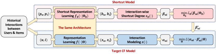
Figure 2. The overall framework of PopGo.

2.1. Conventional Learning Paradigm

We focus on item recommendation from implicit feedback (Rendle et al., 2012; Rendle, 2021), where historical behaviors of a user (e.g., views, purchases, clicks) reflect her preference implicitly. Let $\mathcal{U}$ and $\mathcal{I}$ be the sets of users and items, respectively. We denote the historical user-item interactions by $\mathcal{O}^{+}=\{(u,i)|y_{ui}=1\}$, where $y_{ui}$ indicates that user $u$ has adopted item $i$ before. Under such a scenario, only identity information and historical interactions are available to deduce future interactions among users and items.

Towards this end, CF simply assumes that behaviorally similar users would have similar preference for items. Extensive studies (Rendle et al., 2012; Koren, 2008; He et al., 2020) have developed the CF idea and achieved great success. Scrutinizing these CF models, we summarize the common paradigm as a combination of two modules $z_{x}=s\circ f$: representation learning $f(\cdot)$, interaction modeling $s(\cdot)$.

2.1.1. Representation Learning

For a user-item pair $x=(u,i)$, no overlap exists between the user identity $u$ and item identity $i$. This semantic gap hinders the modeling of user preference. One prevalent solution is generating informative representations of users and items, instead of superficial identities. Here we formulate the representation learning module as a function $f(\cdot)$:

(1) $$\textbf{x}_{u},\textbf{x}_{i}=f(x=(u,i)|\Theta),$$

where $\textbf{x}_{u}\in\mathbb{R}^{d}$ and $\textbf{x}_{i}\in\mathbb{R}^{d}$ are the $d$-dimensional representations of user $u$ and item $i$ respectively, which are expected to delineate their intrinsic characteristics; $f(\cdot)$ is parameterized with $\Theta$. As a result, this module converts $u$ and $i$ into the same latent space and closes the semantic gap.

One evolution of representation learning is in gradually bringing higher-order connections among users and items together. Earlier studies (e.g., MF (Koren, 2008; Rendle et al., 2012), NMF (He et al., 2017), CMN (Ebesu et al., 2018)) project the identity of each user or item into vectorized embedding individually. Later on, some efforts (e.g., SVD++ (Koren, 2008), FISM (Kabbur et al., 2013), MultVAE (Liang et al., 2018)) view the historical interactions of a user (or item) as her (or its) features and integrate their embeddings into representations. From the perspective of user-item interaction graph, interacted items of a user compose her one-hop neighbors. Recently, some follow-on works (e.g., PinSage (Ying et al., 2018), LightGCN (He et al., 2020)) apply GNNs on the user-item interaction graph holistically to incorporate multi-hop connections into representations.

Discussion. Despite great success, evolving from modeling the single identity, the one-hop connection to the holistic interaction graph amplifies the popularity bias in the training interaction data (Kim et al., 2022; Zhou et al., 2023). Specifically, from the view of information propagation, as active users and popular items appear more frequently than the tails, they will propagate more information to the one- and multi-hop neighbors, thus contributing more to the representation learning (Zhu et al., 2021; Abdollahpouri et al., 2019). In turn, the representations over-emphasize the users and items with high popularity.

2.1.2. Interaction Modeling

Having established user and item representations, we now generate the prediction on the user-item pair $x=(u,i)$. Here we summarize the prediction function $s(\cdot)$ as:

(2) $$\alpha_{ui}=s(\textbf{x}_{u},\textbf{x}_{i}),$$

where $\alpha_{ui}\in\mathbb{R}$ reflects how likely user $u$ would adopt item $i$. Typically, $s(\cdot)$ casts the predictive task as estimating the similarity between user representation $\textbf{x}_{u}$ and item representation $\textbf{x}_{i}$. While neural networks like multilayer perceptron (MLP) are applicable in implementing $s(\cdot)$ (He et al., 2017), recent studies (Rendle et al., 2020; Rendle, 2021) suggest that simple functions, such as inner product ${\textbf{x}}^{\top}_{u}\textbf{x}_{i}$, are more suitable for real-world scenarios, due to the simplicity and efficiency. To further convert the inner product into the probability of $u$ selecting $i$, we can resort to cosine similarity ${\textbf{x}}^{\top}_{u}\textbf{x}_{i}/(\left\lVert\textbf{x}_{u}\right\rVert\cdot\left\lVert\textbf{x}_{i}\right\rVert)$ or sigmoidal inner product $1/(1+\exp{({\textbf{x}}^{\top}_{u}\textbf{x}_{i})})$.

To optimize the model parameters, the current CF models mostly opt for the supervised learning objective. Mainstream objectives can be categorized into three groups: pointwise loss (e.g., binary cross-entropy (He et al., 2017)), pairwise loss (e.g., BPR (Rendle et al., 2012)), and softmax loss (Rendle, 2021). Here we minimize sampled softmax loss (Wu et al., 2021) to encourage the predictive score of each observed pair, while stifling that of unobserved pairs as follows:

(3) $$\min_{\Theta}\mathbf{\mathop{\mathcal{L}}}_{0}=-\sum_{(u,i)\in\mathcal{O}^{+}}\log\frac{\exp{(\alpha_{ui}/\tau)}}{\sum_{j\in\mathcal{N}^{+}_{u}}\exp{(\alpha_{uj}/\tau)}},$$

where $(u,i)\in\mathcal{O}^{+}$ is one observed interaction of user $u$, while $\mathcal{N}_{u}=\{j|y_{uj}=0\}$ is the sampled unobserved items that $u$ did not interact with before, and $\mathcal{N}^{+}_{u}=\{i\}\cup{\mathcal{N}_{u}}$; $\tau$ is the hyper-parameter known as the temperature in softmax.

Discussion. Nonetheless, the learning objective is easily influenced by the popularity bias of the training interactions. Obviously, active users and popular items dominate the historical interactions $\mathcal{O}^{+}$. As a result, a lower loss can be naively achieved by recommending popular items (Wei et al., 2021) — the loss will optimize the model parameters towards the pairs with high popularity and inevitably influence the representations via backpropagation (Zhu et al., 2021, 2020).

2.2. Popularity Distribution Shift

Here we get inspiration from the recent studies on OOD (Wiles et al., 2022; Ye et al., 2022) and take a closer look at the popularity of a user $u$, termed $d_{u}$. Formally, we denote the popularity distributions by $p_{\text{train}}(d_{u})$ and $p_{\text{test}}(d_{u})$, which statistically summarize the numbers of $u$-involved interactions on the training and test sets, respectively. Analogously, given an item $i$, we can get the popularity distributions $p_{\text{train}}(d_{i})$ and $p_{\text{test}}(d_{i})$. As the future interactions are unseen during the training time, it is unrealistic to ensure the future (test) data distributions conform to the training data. Thus, the popularity distribution shifts easily arises:

(4) $$p_{\text{train}}(d_{u})\neq p_{\text{test}}(d_{u}),\quad p_{\text{train}}(d_{i})\neq p_{\text{test}}(d_{i}).$$

Worse still, as Equation (3) shows that user and item representations are optimized on the training interactions $\mathcal{O}^{+}$, but are blind to the future (test) interactions $\mathcal{O}^{+}_{\text{test}}$, this learning paradigm is prone to capture the spurious correlations between the popularity and user preference. Taking a user-item pair $(u,i)$ as an example, the spurious correlation arises when the popularity and user preference are strongly correlated at training time, but the testing phase is associated with different correlations since the popularity distribution changes. Such a spurious correlation can be formalized as:

(5) $$p_{\text{train}}(y_{ui}|d_{u},d_{i})\neq p_{\text{test}}(y_{ui}|d_{u},d_{i}),$$

which easily leads to poor generalization (Wiles et al., 2022; Ye et al., 2022). Therefore, it is critical to make CF models robust to such challenges.

2.3. PopGo Debiasing Strategy

As discussed above, the conventional learning paradigm makes both representation learning and interaction modeling modules susceptible to learning popularity bias in the training data as the shortcut. When the test data follows the same distribution as the training data, the popularity shortcut still holds and tricks the CF models in good ID performance. It is much easier to reach a high recommendation accuracy by memorizing the popularity shortcut, instead of probing the actual preference of users. However, in open-world scenarios, the wild test distribution is usually unknown and violates the training distribution, where the popularity shortcut is absent. Hence, the CF models will generalize poorly to the OOD test data.

To enhance the generalization of CF models, it is crucial to alleviate the reliance on popularity shortcuts. Towards this end, PopGo inspects the learning paradigm in Section 2.1 and performs debiasing in both representation learning and interaction modeling components. For the target CF model being debiased, PopGo devises a shortcut model, which has the same architecture as the target CF model, formally $z_{b}=s_{b}\circ f_{b}$, but functions differently: $f_{b}(\cdot)$ focuses on shortcut representation learning, and $s_{b}(\cdot)$ targets at the modeling of interaction-wise shortcut degree. We will elaborate on each component in the following sections.

2.3.1. Shortcut Representation Learning

For a user-item pair $(u,i)$, we denote user popularity and item popularity by $d_{u}$ and $d_{i}$, respectively. Based on the statistics of the training data, $d_{u}$ is the amount of historical items that user $u$ interacted with before, while $d_{i}$ is the amount of observed interactions that item $i$ is involved in. Although such statistical measures can be used as the influence of popularity (Wei et al., 2021; Bell et al., 2008), they are superficial and independent of CF models, thus failing to reflect the changes after the representation learning module $f(\cdot)$ (cf. Section 2.1.1). As a result, the superficial features are insufficient to represent the popularity-relevant information.

Here we devise a function $f_{b}(\cdot)$, which has the same architecture as $f(\cdot)$ but takes the superficial features $b=(d_{u},d_{i})$ as the input. It aims to better encapsulate the popularity-relevant information into shortcut representations:

(6) $$\textbf{b}_{u},\textbf{b}_{i}=f_{b}((d_{u},d_{i})|\Theta_{b}),$$

where $\textbf{b}_{u}\in\mathbb{R}^{d}$ and $\textbf{b}_{i}\in\mathbb{R}^{d}$ separately denote the $d$-dimensional shortcut representations of $u$ and $i$; $\Theta_{b}$ collects the trainable parameters of $f_{b}(\cdot)$.

Assuming MF is the target CF model that projects the one-hot encoding of the user or item identity as an embedding, a separate MF is the shortcut model that maps the one-hot encoding of the user or item frequency into a shortcut embedding. It is worth mentioning that the frequency is treated as a categorical feature, such that the users/items with the same popularity share the identical shortcut embedding. Analogously to the target LightGCN model, an additional LightGCN serves as the shortcut model to create the popularity embedding table and apply the GNN on it to obtain the final shortcut representations. Note that the shortcut representations are different from the conformity embeddings of DICE (Zheng et al., 2021), which are customized for individual users and items and hardly make the best of statistical popularity features. Moreover, with the same target model (e.g., MF, LightGCN), PopGo owns much fewer parameters than DICE.

2.3.2. Interaction-wise Shortcut Modeling

Having obtained shortcut representations of users and items, we now approach the interaction-wise short degree:

(7) $$\beta_{ui}=s_{b}(\textbf{b}_{u},\textbf{b}_{i}),$$

where $\beta_{ui}\in[0,1]$ denotes the probability of user $u$ adopting item $i$, based purely on the popularity-relevant information; $s_{b}(\cdot)$ is defined similarly to $s(\cdot)$ in Equation (2). It is capable of quantifying the effect of the shortcut representations on predicting user preference.

Hereafter, we set softmax loss as the learning objective and minimize it to train the parameters of the shortcut model:

(8) $$\min_{\Theta_{b}}\mathbf{\mathop{\mathcal{L}}}_{b}=-\sum_{(u,i)\in\mathcal{O}^{+}}\log\frac{\exp{(\beta_{ui}/\tau)}}{\sum_{j\in\mathcal{N}^{+}_{u}}\exp{(\beta_{uj}/\tau)}},$$

where $\beta_{uj}$ results from $b^{\prime}=(d_{u},d_{j})$. This optimization enforces the shortcut degree $\beta_{ui}$ to reconstruct the historical interaction, so as to distill useful information — assessing how informative the shortcut representations $\textbf{b}_{u}$ and $\textbf{b}_{i}$ are to predict the interaction. For example, the high value of $\beta_{ui}$ suggests the powerful predictive ability of the popularity shortcut, which easily disturbs the learning of CF models; meanwhile, the low value of $\beta_{ui}$ shows this popularity shortcut is error-prune to predict user preference.

2.3.3. Overall Debiasing

Once the shortcut model is trained, we move forward to debiasing the target CF model. Our intuition is that the debiased model should learn the information beyond those contained in the shortcut model. Specifically, if the shortcut model has already achieved good prediction on a user-item pair, the debiased model should learn beyond the interaction-wise shortcut to preserve the performance; otherwise, it needs to pursue better representations for one observed interaction with a low shortcut degree. In a nutshell, PopGo aims to encourage the target CF model to reduce the reliance on popularity shortcuts and focus more on shortcut-agnostic information.

To this end, given a user-item pair $(u,i)$, we use its interaction-wise shortcut degree $\beta^{*}_{ui}$ as the mask of the prediction $\alpha_{ui}$, formally $\alpha_{ui}\cdot\beta^{*}_{ui}$. On the top of the masked prediction, we minimize the following learning objective to optimize the target CF model, rather than the original loss in Equation (3):

(9) $$\min_{\Theta}\mathbf{\mathop{\mathcal{L}}}=-\sum_{(u,i)\in\mathcal{O}^{+}}\log\frac{\exp{(\alpha_{ui}\cdot\beta^{*}_{ui}/\tau)}}{\sum_{j\in\mathcal{N}^{+}_{u}}\exp{(\alpha_{uj}\cdot\beta^{*}_{uj}/\tau)}},$$

where $\beta^{*}_{ui}$ is the outcome of the well-trained shortcut model. To better interpret the impact of Equation (9) on both representation learning and interaction modeling, we take two user-item pairs, $(u,i)$ and $(u,i^{\prime})$, as an example. Assuming that $\beta^{*}_{ui}\approx 1$ and $\beta^{*}_{ui^{\prime}}\approx 0.2$, $\alpha_{ui}\cdot\beta^{*}_{ui}$ can easily achieve lower loss than $\alpha_{ui^{\prime}}\cdot\beta^{*}_{ui^{\prime}}$, thus making $(u,i)$ and $(u,i^{\prime})$ function as easy and hard instances respectively. To further reduce the losses, $\alpha_{ui^{\prime}}$ needs to pursue higher scores than $\alpha_{ui}$, so as to uncover the popularity-agnostic information. Furthermore, such hard instances offer informative gradients to guide the representation learning towards more robust representations.

The overall framework of PopGo can be summarized as follows:

(10) $$\min_{\Theta}\min_{\Theta_{b}}\mathbf{\mathop{\mathcal{L}}}+\mathbf{\mathop{\mathcal{L}}}_{b}.$$

When the target CF model is trained, we simply disable the shortcut model and deploy $\alpha_{ui}$ for the debiased prediction during inference.

3. Justification

Here we take both causal and information-theoretical look at PopGo.

3.1. Causal Look at PopGo

Throughout the section, an upper-case letter (e.g., $X$) represents a random variable, while its lower-cased letter (e.g., $x$) denotes its observed value.

3.1.1. Causal Graph

Following causal theory (Pearl, 2000; Pearl et al., 2016), we formalize the causal graph of CF in Figure 3, which is consistent with causal graphs summarized in (Chen et al., 2020a). It presents the causalities among three variables: user-item pair $X$, popularity feature $B$, and interaction label $Y$. Each link represents a cause-and-effect relationship between two variables:

• $X\rightarrow B$. The popularity feature $B$ is determined by the user-item pair $X$, which consists of the user popularity and item popularity.

• $X\rightarrow Y\leftarrow B$. The interaction label $Y$ is made based on both user-item pair $X$, and its popularity feature $B$.

Based on the counterfactual notations (Pearl, 2000; Pearl et al., 2016), if $X$ is set as $x$, the value of $B$ is denoted by:

(11) $$B_{x}=B(X=x).$$

For the treatment notation, when setting $X$ on the user-item pair $x=(u,i)$, we have $B_{x}=b=(p_{u},p_{i})$ by looking up its popularity feature. Under no-treatment condition, $B_{x^{*}}$ describes the situation where $X$ is intervened as $x^{*}=\emptyset$. Analogously, if $X$ and $B$ is set as $x$ and $b$ respectively, the value of $Y$ would be represented as:

(12) $$Y_{x,b}=Y(X=x,B=b).$$

In the factual world, we have $Y_{x,B_{x}}$ by setting $X$ as $x=(u,i)$ and naturally obtaining $B_{x}=b=(p_{u},p_{i})$. In the counterfactual world, $Y_{x,B_{x^{*}}}=Y(X=x,B=B(X=x^{*}))$ presents the status where $X$ is set as $x$ and $B$ is set to the value when $X$ had been $x^{*}$. Similarly, $Y_{x^{*},B_{x}}=Y(X=x^{*},B=B(X=x))$.

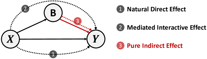
Figure 3. Causal graph of CF, where $X$, $B$, and $Y$ denote the historical user-item interaction, popularity distribution, interaction label, respectively. Considering a specific example of a user $u$ and an item $i$, we can specialize these variables to certain values: $X=(u,i)$ depicting the user and item representations, $B=(p_{u},p_{i})$ summarizing the information about the popularity distribution, $Y=y_{ui}$ indicating how likely $u$ will interact with $i$.

3.1.2. Total Effect vs. Total Direct Effect

Causal effect (Pearl, 2000; Pearl et al., 2016) is the difference between two potential outcomes, when performing two different treatments. Considering that $X=x$ is under treatment, while $X=x^{*}$ is under control, the total effect (TE) of $X=x$ on $Y$ is defined as:

(13) $$\text{TE}=Y_{x,B_{x}}-Y_{x^{*},B_{x^{*}}}=Y_{x,b}-Y_{x^{*},b^{*}}.$$

As such, the conventional learning objective (cf. Equation (3)) in essence maximizes the TE of $X=x$ on $Y$.

TE consists of total direct effect (TDE) and pure indirect effect (PIE) (VanderWeele, 2013), where TDE is composed of mediated interactive effect (MIE) (VanderWeele, 2013) and natural direct effect (NDE) (Robins and Greenland, 1992). Figure 3 illustrates the paths corresponding to different components. Formally, the PIE of $X$ on $Y$ is defined as:

(14) $$\text{PIE}=Y_{x^{*},B_{x}}-Y_{x^{*},B_{x^{*}}}=Y_{x^{*},b}-Y_{x^{*},b^{*}},$$

which reflects how the interaction label changes with the difference of popularity feature solely — under treatment (i.e., $B=B_{x}=B(X=x)$) and control (i.e., $B=B_{x^{*}}=B(X=x^{*})$). Clearly, PIE only captures the influence of popularity features, while ignoring that of user-item pair. However, as the popularity distribution easily varies in open-world scenarios, PIE fails to suggest user preference reliably. We hence attribute the CF models’ poor generalization to memorizing PIE as the shortcut.

We now inspect the TDE of $X$ on $Y$:

(15) $$\text{TDE}=Y_{x,B_{x}}-Y_{x^{*},B_{x}}=Y_{x,b}-Y_{x^{*},b},$$

which represents how the interaction label responses with the change of user-item pair — under treatment (i.e., $X=x=(u,i)$) and control (i.e., $X=x^{*}=\emptyset$). Distinct from PIE, TDE reflects the critical information inherent in the user-item pair, which is useful to estimate user preference. It is worth mentioning that, as a part of TDE, MIE contains a good impact of popularity, rather than discarding all information relevant to popularity.

3.1.3. Parameterization & Training

Therefore, we expect the target CF models to exclude PIE and emphasize TDE. However, it is hard to optimize TDE directly. Here we parameterize the estimation of $Y$ as a log-likelihood of the combination of components:

(16) $$Y(X,B)=\log{(Z_{X}\cdot Z_{B})},$$

where $Z_{B}$ is the shortcut model that only takes the popularity-only features, and $Z_{X}$ is the target CF model founded upon the user-item pairs and supposes to make unbiased predictions with debiased representations. Wherein, $Z_{B}$ is represented as:

(17) $$Z_{B}=\begin{cases}z_{b}=\beta_{ui},&\text{if}~{}~{}B=b\\ z^{*}_{b}=c_{1},&\text{if}~{}~{}B=\emptyset\end{cases},$$

where $B=b=(p_{u},p_{i})$ is the treatment condition, while $B=b^{*}=\emptyset$ is the control condition. As the shortcut model cannot deal with the invalid input $\emptyset$, we assume that it will return a constant $c_{1}$ as the probability. In contrast, under condition of treatment $B=b$, the shortcut model will yield the probability $\beta_{ui}$ (cf. Equation (7)). $Z_{X}$ is represented as:

(18) $$Z_{X}=\begin{cases}z_{x}=\alpha_{ui},&\text{if}~{}~{}X=x\\ z^{*}_{x}=c_{2},&\text{if}~{}~{}X=\emptyset\end{cases},$$

where $X=x=(u,i)$ and $X=x^{*}=\emptyset$ indicate $X$ under treatment and control, respectively. When $X=x$, the CF model generates the probability $\alpha_{ui}$ (cf. Equation (2)); meanwhile, the invalid input $\emptyset$ is assigned with the constant probability $c_{2}$.

According to Equations (16), (17), and (18), we can quantify each term within TE, PIE, and TDE, such as $Y_{x,b}=\log{(z_{x}\cdot z_{b})}$. However, directly maximizing TDE is hard to harness the CF model to disentangle the popularity-relevant and popularity-agnostic information. Our PopGo strategy first maximizes PIE and then maximizes TE to get TDE. Specifically, optimizing the shortcut model via Equation (8) is consistent with learning the PIE maximum:

(19) $$\max_{\beta_{ui}}\text{PIE}=\log{(c_{2}\cdot\beta_{ui})}-\log{(c_{2}\cdot c_{1})}=\log{\beta_{ui}}-\log{c_{1}}.$$

Once the shortcut model is well-trained, we use its outcome $\beta^{*}_{ui}$ to maximize TE, which aligns well with Equation (9):

(20) $$\max_{\alpha_{ui}}\text{TE}=\log{(\alpha_{ui}\cdot\beta^{*}_{ui})}-\log{(c_{2}\cdot c_{1})}.$$

As a consequence, it is capable of guiding the CF models to compute TDE and get rid of PIE, which is the cause of poor generalization w.r.t. popularity distribution. In summary, PopGo enforces the shortcut model and the CF model to fall into the roles of estimating PIE and TDE separately.

3.2. Information-Theoretical Look at PopGo

From the perspective of information theory (Kullback, 1997), the conventional learning paradigm of CF models (cf. Equation (3)) essentially maximizes the mutual information $I(X;Y)$ between the user-item pair variable $X$ and the label variable $Y$. However, as the popularity feature $B$ is inherent in the interaction $X$ — that is, $B$ is a descendant of $X$ in Figure 3, maximizing $I(X;Y)$ fails to shield the CF models from the popularity shortcut.

We will show that PopGo maximizes the conditional mutual information $I(X;Y|B)$ instead. Intuitively, conditioning on a variable means fixing the variations of this variable, and hence its effect can be removed (Kullback, 1997). Hence, $I(X;Y|B)$ measures the information amount contained in $X$ to predict $Y$, when conditioning on $B$ and removing its effect. Towards this end, we elaborate on the purpose of each step in PopGo.

First, to optimize the shortcut model, PopGo minimizes Equation (8) which is equivalent to maximizing the mutual information between the popularity variable $B$ and the interaction label variable $Y$. Formally, negative $\mathbf{\mathop{\mathcal{L}}}_{b}$ in Equation (8) is a lower bound of $I(B;Y)$:

(21) $$-\mathbf{\mathop{\mathcal{L}}}_{b}=-H(Y|B)\leq I(B;Y),$$

where $I(B;Y)=H(Y)-H(Y|B)$ quantifies the information amount of $Y$ by observing $B$ solely; $H(Y|B)$ is the conditional entropy, and $H(Y)$ is the marginal entropy. The optimal critic of minimizing $\mathbf{\mathop{\mathcal{L}}}_{b}$, $\beta^{*}_{ui}$, is a log-likelihood (Poole et al., 2019): $\beta^{*}_{ui}=\log{(p(y=1|b))}+c$, where $c$ is the constant.

Hereafter, to optimize the target CF model, PopGo minimizes Equation (9), which is consistent with maximizing the mutual information between $(X,B)$ and $Y$. Analogously, $-\mathbf{\mathop{\mathcal{L}}}$ of Equation (9) serves as a lower bound of $I(X,B;Y)$:

(22) $$-\mathbf{\mathop{\mathcal{L}}}=-H(Y|X,B)\leq I(X,B;Y),$$

where $I(X,B;Y)$ assesses the amount of information about $Y$ by observing $X$ and $B$ jointly. When using $\beta^{*}_{ui}=\log{(p(y=1|b))}+c$ and $\frac{1}{\mathcal{N}^{+}_{u}}\sum_{j\in\mathcal{N}^{+}_{u}}p(y=1|b^{\prime})$ to estimate the marginal distribution $p(y=1)=\int p(b^{\prime})p(y=1|b^{\prime})db^{\prime}$, we further rewrite $-\mathbf{\mathop{\mathcal{L}}}$ as follows:

$$-\mathbf{\mathop{\mathcal{L}}} \approx\sum_{(u,i)\in\mathcal{O}^{+}}\log{\frac{\exp{(\alpha_{ui}/\tau)}}{\sum_{j\in\mathcal{N}^{+}_{u}}p(y=1|b^{\prime})\exp{(\alpha_{uj}/\tau)}}}$$

(23) $$+\sum_{(u,i)\in\mathcal{O}^{+}}\log{\frac{p(y=1|b)}{p(y=1)}},$$

where the second term is the estimation of $I(B;Y)$. As $I(X,B;Y)=I(X;Y|B)+I(B;Y)$ based on the information theory, the first term approaches the desired conditional mutual information $I(X;Y|B)$. In summary, PopGo encourages the shortcut model and the target CF model to maximize $I(B;Y)$ and $I(X;Y|B)$, respectively.

4. Experiments

In this section, we provide empirical results to demonstrate the effectiveness of PopGo and answer the following research questions:

• RQ1: How does PopGo perform compared with the state-of-the-art debiasing strategies in both OOD and ID test evaluations?

• RQ2: What are the impacts of the components (e.g., the value of temperature parameter, the shortcut model) on PopGo? Can PopGo truly pursue high-quality debiased representations?

4.1. Experimental Settings

Datasets. We conduct experiments on six real-world benchmark datasets: Yelp2018 (He et al., 2020), Tencent (Yuan et al., 2020), Amazon-Book (He and McAuley, 2016), Alibaba-iFashion (Chen et al., 2019), Douban Movie (Song et al., 2019), and Yahoo!R3 (Marlin and Zemel, 2009). To ensure the data quality, we adopt the 10-core setting (He and McAuley, 2016), where each user and item have at least ten interaction records. Table 1 summarizes the detailed dataset statistics.

Data Splits for ID and OOD Evaluations. Typically, each dataset is partitioned into three parts: training, validation, and test sets. The existing debiasing methods (Liang et al., 2016; Wei et al., 2021; Zheng et al., 2021) mostly assume that either the test distribution is known in advance or the validation and test sets have the same or similar distribution, which is at odds with the training set. Such assumptions cause the leakage of OOD test information during training the model or tuning the hyperparameters in the validation set. However, the OOD distribution is usually unknown in the wild and open-world scenarios. To make the evaluation more practical, we follow the standard settings of recent generalization studies (Teney et al., 2020; Niu and Zhang, 2021) and create test evaluations on ID and OOD settings on Yelp2018, Tencent, Amazon-Book, and Alibaba-iFashion Datasets. Specifically, we split each dataset into four parts: training, ID validation, ID test, and OOD test sets. To build the OOD test set, we randomly sample $20\%$ of interactions with equal probability w.r.t. items, which are regarded as the most extreme balanced recommendation under an entirely random policy (Liang et al., 2016; Wei et al., 2021; Schnabel et al., 2016). We then randomly split the remaining interactions into $50\%$ for training, $10\%$ for ID validation, and $20\%$ for ID test sets. As such, the uniform distribution in the OOD test differs from the long-tailed distribution in training, ID validation, and ID test sets. Furthermore, we report the KL-divergence between the item popularity distribution of each set and the uniform distribution in Table 1. A larger KL-divergence value indicates that the heavier portion of interactions concentrates on the head of distribution.

Temporal Data Splits. In many applications, the distribution of popularity changes over time. To evaluate the generalization of PopGo w.r.t. temporal distribution shift, we also employ the standard temporal splitting strategy (Boratto et al., 2021) on Douban Movie (Song et al., 2019) and chronologically slice the user-item interactions into the training, validation, and test sets (70%:10%:20%) based on the timestamps. Unbiased Data Splits. The inherent missing-not-at-random condition in real-world recommender systems makes offline evaluation of collaborative filtering a recognized challenge. To address this, the Yahoo!R3 (Marlin and Zemel, 2009), providing unbiased test sets collected following the missing-complete-at-random (MCAR) principle, is widely employed. Specifically, the training data of Yahoo!R3, typically biased, includes user-selected item ratings. In contrast, the testing data is gathered from online surveys where users rate items chosen at random.

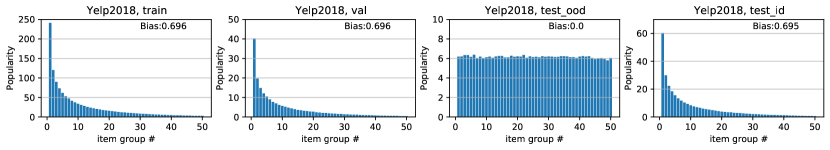
(a) Yelp2018.

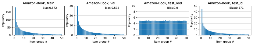
(b) Amazon-Book.

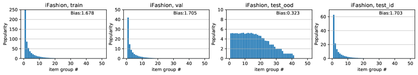
(c) Alibaba-iFashion.

Figure 4. Histogram of the Training, Validation, OOD testing, and ID testing sets for the Yelp2018, Amazon-Book, and Alibaba-iFashion datasets.

Table 1. Dataset statistics.

	Douban	Yelp2018	Tencent	Amazon-Book	iFashion	Yahoo!R3
#Users	36,644	31,688	95,709	52,643	300,000	14,382
#Items	22,226	38,048	41,602	91,599	81,614	1,000
#Interactions	5,397,926	1,561,406	2,937,228	2,984,108	1,607,813	129,748
Sparsity	0.00663	0.00130	0.00074	0.00062	0.00007	0.00902
$D_{KL}$-Train	1.471	0.713	1.735	0.684	2.119	0.854
$D_{KL}$-Validation	1.642	0.713	1.733	0.684	2.123	0.822
$D_{KL}$-Test_OOD	-	0.000	0.015	0.000	0.435	-
$D_{KL}$-Test_ID	-	0.713	1.734	0.683	2.121	-
$D_{KL}$-Test_temporal	1.428	-	-	-	-	-
$D_{KL}$-Test_unbiased	-	-	-	-	-	0.002

Table 2. Additional Parameter statistics of PopGo.

	Yelp2018	Tencent	Amazon-Book	Alibaba-iFashion	Yahoo!R3
User Pop Embed.	450*64	327*64	72*64	94*64	82*64
Item Pop Embed.	415*64	396*64	882*64	545*64	239*64

Evaluation Metrics. In the evaluation phase, we conduct the all-ranking strategy (Krichene and Rendle, 2020), rather than sampling a subset of users (Wang et al., 2019b; Wang et al., 2020). More specifically, each observed user-item interaction is a positive instance, while an item that the user did not adopt before is randomly sampled to pair the user as a negative instance. All these items are ranked based on the predictions of the recommender model. To evaluate top recommendation, three widely used metrics (He et al., 2020; Krichene and Rendle, 2020; He et al., 2017; Wei et al., 2021; Zheng et al., 2021) are reported by averaging: Hit Ratio (HR), Recall and Normalized Discounted Cumulative Gain (NDCG) cut at $K$, where $K$ is set as 20 by default.

Baselines. We select two high-performing CF models, matrix factorization (MF) (Rendle et al., 2012; Koren, 2008) and LightGCN (He et al., 2020), to debias, which are the representative of conventional and state-of-the-art backbone models. To demonstrate the broad applicability and superior performance of our proposed PopGo, we conduct additional experiments using the popular CF backbone - UltraGCN (Mao et al., 2021). For adequate comparisons, we compare PopGo with high-performing in-processing debiasing strategies in almost all research directions, including Inverse Propensity Score method (IPS-CN (Gruson et al., 2019)), domain adaption method (CausE (Bonner and Vasile, 2018)), causal embedding method (DICE (Zheng et al., 2021), MACR (Wei et al., 2021)), and regularization-based method (SAM-REG (Boratto et al., 2021)).

• MF (Rendle et al., 2012): Matrix Factorization (MF) is a classical CF method that uses user and item identity representations to predict, optimized by the Bayesian Personalized Ranking (BPR) loss.

• LightGCN (He et al., 2020): LightGCN is the state-of-the-art CF model that learns user and item representations by linearly propagating embeddings on the user-item interaction graph and weighted summing them as the final representations.

• UltraGCN (Mao et al., 2021): UltraGCN is an ultra-simplified version of Graph Convolutional Networks (GCNs) designed for efficient recommendation systems. It skips the traditional message-passing mechanism, which can slow training, and approximates the limit of infinite-layer graph convolutions using a constraint loss.

• IPS-CN (Gruson et al., 2019): IPS family of methods (Schnabel et al., 2016; Joachims et al., 2018; Bottou et al., 2013) eliminate popularity bias by re-weighting each instance according to item popularity. IPS-CN further adds normalization to achieve lower variance at the expense of a higher bias.

• CausE (Bonner and Vasile, 2018): CausE is a domain adaptation algorithm that requires one biased and one unbiased dataset to benefit its recommendation. Our experiments separate the training set into a 10% debiased uniform training set (same as our OOD test distribution) and a 90% biased training set.

• DICE (Zheng et al., 2021): Dice learns disentangled causal embeddings for interest and conformity by training with cause-specific data according to the collider effect in causal inference.

• MACR (Wei et al., 2021): MACR performs counterfactual inference to remove the popularity bias by estimating and eliminating the direct effect from the item node to the prediction score.

• SAM-REG (Boratto et al., 2021): SAM-REG consists of two components: the training examples mining balances the distribution of observed and unobserved items, and the regularized optimization minimizes the biased correlation between predicted user-item relevance and item popularity.

Table 3. Overall performance comparison in OOD test. The improvement achieved by PopGo is significant ($p$-value $<<$ 0.05).

OOD test	Yelp2018			Tencent
	HR@20	Recall@20	NDCG@20	HR@20	Recall@20	NDCG@20
ItemPop	0.0031	0.0003	0.0007	0.0016	0.0002	0.0004
MF	0.0558	0.0064	0.0133	0.0258	0.0047	0.0069
+ IPS-CN	0.0697	0.0091	0.0189	0.0359	0.0067	0.0096
+ CausE	0.0651	0.0073	0.0148	0.0283	0.0049	0.0070
+ DICE	0.0681	0.0068	0.0161	0.0380	0.0060	0.0085
+ SAM-REG	0.0731*	0.0088	0.0173	0.0386*	0.0070	0.0101
+ MACR	0.0696	0.0076	0.0152	0.0278	0.0066	0.0077
+ PopGo	0.0728	0.0095*	0.0192*	0.0371	0.0072*	0.0103*
Imp. %	-0.41%	4.40%	1.59%	-3.89%	2.86%	1.98%
LightGCN	0.0558	0.0069	0.0141	0.0213	0.0044	0.0054
+ IPS-CN	0.0664	0.0084	0.0153	0.0295	0.0063	0.0082
+ CausE	0.0655	0.0082	0.0163	0.0269	0.0054	0.0064
+ DICE	0.0651	0.0079	0.0161	0.0414	0.0046	0.0104
+ SAM-REG	0.0862	0.0108	0.0213	0.0425	0.0076	0.0101
+ MACR	0.0711	0.0092	0.0164	0.0350	0.0081	0.0082
+ PopGo	0.1102*	0.0151*	0.0231*	0.0426*	0.0085*	0.0113*
Imp. %	21.78%	39.81%	8.54%	0.24%	4.94%	8.65%
	Amazon-book			Alibaba-iFashion
	HR@20	Recall@20	NDCG@20	HR@20	Recall@20	NDCG@20
ItemPop	0.0013	0.0001	0.0004	0.0003	0.0008	0.0001
MF	0.0699	0.0104	0.0195	0.0077	0.0039	0.0022
+ IPS-CN	0.0856	0.0135	0.0237	0.0095	0.0050	0.0027
+ CausE	0.0464	0.0050	0.0106	0.0050	0.0023	0.0012
+ DICE	0.0749	0.0091	0.0204	0.0088	0.0047	0.0024
+ SAM-REG	0.0917	0.0141	0.0279	0.0127	0.0067	0.0031
+ MACR	0.0919	0.0155	0.0249	0.0075	0.0037	0.0016
+ PopGo	0.0981*	0.0162*	0.0297*	0.0146*	0.0076*	0.0038*
Imp. %	6.75%	4.52%	6.45%	14.96%	13.43%	22.58%
LightGCN	0.0782	0.0117	0.0208	0.0069	0.0033	0.0014
+ IPS-CN	0.1015	0.0167	0.0304	0.0080	0.0038	0.0017
+ CausE	0.0831	0.0133	0.0217	0.0063	0.0028	0.0012
+ DICE	0.0700	0.0086	0.0186	0.0091	0.0043	0.0020
+ SAM-REG	0.1049	0.0157	0.0295	0.0110	0.0050	0.0028
+ MACR	0.0990	0.0146	0.0267	0.0072	0.0037	0.0017
+ PopGo	0.1332*	0.0232*	0.0398*	0.0164*	0.0093*	0.0040*
Imp. %	26.98%	38.92%	30.92%	49.09%	86.00%	42.86%

Table 4. Overall performance comparison in ID test. The improvement achieved by PopGo is significant ($p$-value $<<$ 0.05).

ID test	Yelp2018			Tencent
	HR@20	Recall@20	NDCG@20	HR@20	Recall@20	NDCG@20
ItemPop	0.0920	0.0175	0.0184	0.1639	0.0384	0.0274
MF	0.3650	0.0801	0.1042	0.2988	0.0874	0.0871
+ IPS-CN	0.3415	0.0735	0.0902	0.2296	0.0663	0.0574
+ CausE	0.2820	0.0558	0.0793	0.2410	0.0648	0.0750
+ DICE	0.1760	0.0281	0.0410	0.2579	0.0736	0.0782
+ SAM-REG	0.2431	0.0458	0.0622	0.1500	0.0406	0.0419
+ MACR	0.2090	0.0469	0.0531	0.1648	0.0479	0.0445
+ PopGo	0.4504*	0.1075*	0.1419*	0.4042*	0.1279*	0.1286*
Imp. %	23.40%	34.21%	36.18%	35.27%	46.31%	47.73%
LightGCN	0.4124	0.0938	0.1210	0.3547	0.1067	0.1067
+ IPS-CN	0.3548	0.0771	0.103	0.2844	0.0811	0.0878
+ CausE	0.3905	0.0874	0.1172	0.3294	0.0966	0.1053
+ DICE	0.1714	0.0335	0.0418	0.2443	0.0483	0.0683
+ SAM-REG	0.3180	0.0657	0.0893	0.2279	0.0653	0.0663
+ MACR	0.2650	0.0490	0.0832	0.2925	0.0830	0.0967
+ PopGo	0.4376*	0.1037*	0.1402*	0.3974*	0.1178*	0.1286*
Imp. %	6.11%	10.55%	15.87%	12.04%	10.92%	20.52%
	Amazon-book			Alibaba-iFashion
	HR@20	Recall@20	NDCG@20	HR@20	Recall@20	NDCG@20
ItemPop	0.0639	0.0102	0.0104	0.0348	0.0212	0.0063
MF	0.3621	0.0825	0.1102	0.0912	0.0603	0.0260
+ IPS-CN	0.3361	0.0753	0.0970	0.0817	0.0558	0.0212
+ CausE	0.2578	0.0486	0.0736	0.0566	0.0369	0.0147
+ DICE	0.2997	0.0645	0.0902	0.0630	0.0380	0.0185
+ SAM-REG	0.2727	0.0599	0.0815	0.0455	0.0305	0.0126
+ MACR	0.2510	0.0549	0.0711	0.0862	0.0557	0.0253
+ PopGo	0.4433*	0.1081*	0.1481*	0.1540*	0.1050*	0.0475*
Imp. %	22.42%	31.08%	34.39%	36.40%	37.98%	37.28%
LightGCN	0.3825	0.0891	0.1224	0.1154	0.0754	0.0318
+ IPS-CN	0.3617	0.0834	0.1149	0.0986	0.0657	0.0276
+ CausE	0.3862	0.0981	0.1277	0.0421	0.0435	0.0194
+ DICE	0.2140	0.0450	0.0630	0.1092	0.0747	0.0315
+ SAM-REG	0.3382	0.0773	0.1080	0.0748	0.0502	0.0229
+ MACR	0.3331	0.0733	0.1082	0.0770	0.0497	0.0235
+ PopGo	0.4362*	0.1101*	0.1575*	0.1491*	0.1023*	0.0472*
Imp. %	12.95%	12.23%	23.34%	29.20%	35.68%	48.43%

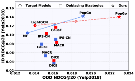
(a) Yelp2018.

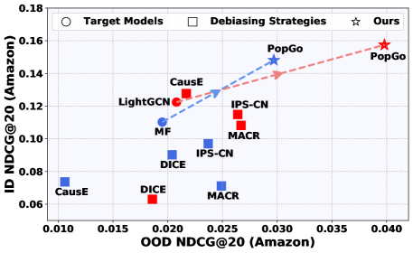
(b) Amazon-Book.

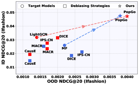
(c) Alibaba-iFashion.

Figure 5. Performance of debiasing strategies on the Yelp2018, Amazon-Book, and Alibaba-iFashion datasets.

4.2. Detailed Experimental Settings

Parameter Settings. We implement our PopGo in TensorFlow. Our codes, datasets, and hyperparameter settings are available at https://github.com/anzhang314/PopGo to guarantee reproducibility. All experiments are conducted on a single Tesla-V100 GPU. For a fair comparison, all methods are optimized by Adam (Kingma and Ba, 2015) optimizer with the embedding size as 64, learning rate as 1e-3, max epoch of 400, and the coefficient of regularization as 1e-5 in all experiments. The batch size on Yelp2018, Tencent, Amazon-Book, and Douban is 2048, while the batch size for MF-based models on iFashion is set to 256 to avoid bad convergence. Following the default setting in (He et al., 2020), the number of embedding layers for LightGCN is set to 2. We adopt the early stop strategy that stops training if Recall@20 on the validation set does not increase for 10 successive epochs. A grid search is conducted to tune the critical hyperparameters of each strategy to choose the best models w.r.t. Recall@20 on the validation set.

For PopGo, we can search the $\tau$ in a wide range to obtain the best performance. But in this paper, across all datasets, we report $\tau=0.07$. We emphasize that the performance of PopGo can be further improved through a finer grid search in the specific dataset as shown in Section 4.4.1. The pre-training stage for the shortcut models is set to 5 epochs, then is frozen afterward. Negative sampling size is set to 64 for PopGO-MF, while inbatch-negative sampling is used for PopGO-LightGCN to reduce time for training. The size of additional parameters compared with MF that comes from the shortcut model is listed in Table 2.

For IPS-CN, we follow the paper (Zheng et al., 2021) to add re-weighting factors. For CausE, 10% of training data with uniform distribution is used as the intervened set. The counterfactual penalty factor $cf\_pen$ is tuned in the range of $[0.01,0.1]$ and $cf\_pen=0.05$ are reported for best overall performance. For MACR, we follow the original settings (Wei et al., 2021) to set weights for user branch $\alpha=1e-3$ and item branch $\beta=1e-3$ respectively. We further tune hyperparameter $c=0,10,20,30,40,50$. Notice that directly tuning hyper-parameter for best validation performance(ID) leads to small $c$, which degenerates MACR to backbone model with no debiasing effect. Therefore, we manually fix $c=40$ for overall best performance. For SAM-REG, we follow the default setting (Boratto et al., 2021) by setting $rweight=0.05$. For DICE, we set conformity loss $\alpha=0.1$ and discrepancy loss $\beta=0.01$ respectively, and set margin decay and loss decay to 0.9. The margin value is set for different datasets (10 for Amazon-book, Tencent, and Yelp2018, 2 for iFashion) according to the mean and median of item popularity for best performance.

Table 5. Effect of shortcut model on PopGo.

		Yelp2018				Tencent
		OOD Test		ID Test		OOD Test		ID Test
		Recall@20	NDCG@20	Recall@20	NDCG@20	Recall@20	NDCG@20	Recall@20	NDCG@20
MF	PopGo	0.1050	0.0475	0.0095	0.0192	0.1075	0.1419	0.0072	0.0103
	PopGo-S	0.0761	0.0346	0.0081	0.0172	0.0891	0.1207	0.0054	0.0082
	Imp. %	40.0%	37.3%	17.3%	11.6%	20.7%	17.56%	33.3%	25.6%
LightGCN	PopGo	0.1023	0.0472	0.0151	0.0230	0.1037	0.1402	0.0085	0.0113
	PopGo-S	0.0704	0.0324	0.0101	0.0184	0.0800	0.1125	0.0057	0.0075
	Imp. %	31.2%	33.7%	49.5%	25.0%	29.6%	24.6%	49.1%	50.7%
		Amazon-Book				Alibaba-iFashion
		OOD Test		ID Test		OOD Test		ID Test
		Recall@20	NDCG@20	Recall@20	NDCG@20	Recall@20	NDCG@20	Recall@20	NDCG@20
MF	PopGo	0.1279	0.1286	0.0162	0.0297	0.1081	0.1481	0.0076	0.0038
	PopGo-S	0.1125	0.1175	0.0136	0.0268	0.1042	0.1468	0.0047	0.0024
	Imp. %	13.7%	9.45%	19.1%	10.8%	3.7%	0.9%	61.7%	58.3%
LightGCN	PopGo	0.1178	0.1286	0.0232	0.0398	0.1101	0.1575	0.0083	0.0040
	PopGo-S	0.0981	0.1096	0.0188	0.0320	0.1008	0.1441	0.0041	0.0022
	Imp. %	20.1%	17.3%	23.4%	24.4%	9.2%	9.3%	97.6%	81.8%

Table 6. The performance comparison on Douban dataset.

	MF			LightGCN
	HR@20	Recall@20	NDCG@20	HR@20	Recall@20	NDCG@20
Backbone	0.2924	0.0294	0.0472	0.3543	0.0313	0.0602
+ IPS-CN	0.2514	0.0174	0.0324	0.3212	0.0261	0.0502
+ CausE	0.2725	0.0203	0.0376	0.3403	0.0275	0.0514
+ SAM-REG	0.2826	0.0191	0.0390	0.2944	0.0252	0.0488
+ MACR	0.1084	0.0087	0.0163	0.3127	0.0271	0.0519
+ PopGo	0.3776*	0.0333*	0.0613*	0.3613*	0.0349*	0.0660*
Imp. %	29.1%	13.3%	29.9%	2.0%	11.5%	9.7%

Table 7. Performance comparison in the unbiased test under UltraGCN backbone.

	Yahoo!R3
	HR@20	Recall@20	NDCG@20
UltraGCN	0.1972	0.1309	0.0599
+ IPS-CN	0.1997	0.1315	0.0595
+ CausE	0.2060	0.1324	0.0619
+ SAM-REG	0.1964	0.1292	0.0583
+ MACR	0.2023	0.1319	0.0591
+ PopGo	0.2161*	0.1403*	0.0635*

Table 8. Training cost on Tencent (seconds per epoch/total).

	Backbone	+IPS-CN	+CausE	+DICE	+SAM-REG	+MACR	+PopGO
MF	15.5/17887	17.8/10662	16.6/1859	66.7/38152	18.2/3458	160/17600	35.1/2141
LightGCN	78.6/4147	108/23652	47.2/3376	126/6804	49.8/10458	135/20250	141/3102

4.3. Performance Comparison (RQ1)

Table 3 and Table 4 report the comparison of debiasing performance in OOD and ID test evaluations, respectively. Wherein the best performing methods are bold and starred, and the strongest baselines are underlined; Imp.% measures the relative improvements of PopGo over the strongest baselines. We observe that:

• In both OOD and ID evaluations, PopGo significantly outperforms the baselines across four datasets in most cases. Specifically, it achieves remarkable improvements over the best debiasing baselines and target CF models by 1.59% - 42.86% and 15.87% - 48.43% w.r.t. NDCG@20 in OOD and ID settings, respectively. Clearly, PopGo is not only superior to the debiasing strategies in the OOD settings but also performs better than the original CF models in the ID settings. This verifies that PopGo improves the generalization of backbones, rather than seeking a trade-off between ID and OOD performance.

• Jointly analyzing the debiasing baselines in Tables 3, 4 and Figure 1(b), there is a trade-off trend between the ID and OOD performance. Generally, with the increase of OOD results, their ID performance is becoming worse. We conjecture that their OOD improvements may come from the sacrifice of ID performance, thus they might generalize poorly in the wild.

• PopGo is able to capture the model-dependent popularity bias. Specifically, over other debiasing strategies, the improvements achieved by LightGCN+PopGo are more significant than that by MF+PopGo. As discussed in Section 2.1, LightGCN could amplify the bias during the information propagation, thus owning stronger biases than MF. It inspires us to reduce the potential biases caused by the model architecture. By cloning the target CF model as the shortcut model (cf. Section 2.3.1), our PopGo can package the model-dependent bias into the shortcut representations and represent the bias via the interaction-wise shortcut degree more accurately.

• Debiasing baselines perform unstably across datasets. For example, in Alibaba-iFashion, the OOD results of MF+CausE, MF+MACR, and MF+DICE are lower than MF w.r.t. all metrics. Compared with other datasets, Alibaba-iFashion is the sparsest and most biased, making it more challenging to be debiased. Without an effective measurement of interaction-wise shortcut degrees or the OOD test prior to painstakingly tune the hyperparameters, the debiasing ability of these baselines is limited. In contrast, benefiting from no assumption on the test data, PopGo can attain remarkable improvements ($40\%$ - $100\%$ on Alibaba-iFahsion) in the OOD setting.

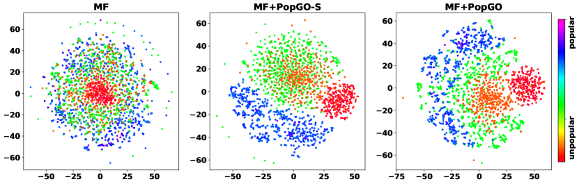
Figure 8. T-SNE (Van der Maaten and Hinton, 2008) visualization of item representations.

• PopGo can leverage the popularity information to boost the ID performance. Interaction sparsity influences the representation quality of the target models. As the sparsity increases across datasets, PopGo significantly promotes the ID performance compared with the non-debiased backbones in most cases. Here we attribute this to (1) the MIE of popularity captured by PopGo, from the causal-theoretical view; and (2) the focus on mining the hard examples that are with sparser interactions (See the visual evidence in Figure 8).

Moreover, Table 8 shows the training time of all methods, where PopGo has the comparable time complexity to the backbone models. Furthermore, Table 6 elaborates the comparison of performance on the temporal split dataset, Douban Movie. Table 7 presents a comparative analysis of debiasing performance in unbiased test evaluations, Yahoo!R3. We observe that:

• PopGo consistently outperforms all baselines in terms of all metrics on Douban Movie. For instance, it achieves significant gains over the target models - MF and LightGCN w.r.t. NDCG@20 by 29.9% and 9.7%, respectively. We attribute these results to successfully improving the generalization of target CF models against the popularity distribution shift over time.

• None of the debiasing baselines could maintain a comparable performance to the original CF models on temporal split settings. Surprisingly, even the state-of-the-art popularity debiasing technique - MACR, fails to diagnose the popularity bias when the bias changes over time. We ascribe the failure to their disability of measuring instance-wise popularity bias and the trade-off of sacrificing accuracy to promote item coverage.

• PopGo consistently surpasses other debiasing methods and the UltraGCN backbone model in unbiased evaluations on Yahoo!R3. Notably, some debiasing methods, such as MACR and SAM-REG, may even reduce recommendation accuracy. This suggests that PopGo effectively mitigates popularity bias and exhibits wider applicability in real-world scenarios.

4.4. Study on PopGo (RQ2)

4.4.1. Impact of Temperature $\tau$

PopGo only has one hyperparameter to tune — temperature $\tau$ in Equation (8) and (9). In Figure 6, we report the sensitivity analysis of $\tau$ on Tencent and find:

• Both OOD and ID evaluations exhibit the concave unimodal functions of $\tau$, where the curves reach the peak almost synchronously in a small range of $\tau$. For example, MF+PopGo gets the best performance when $\tau=0.06$ and $\tau=0.07$ in OOD and ID settings, respectively. This justifies that PopGo does not suffer from the trade-off between the OOD and ID evaluations, and again verifies that PopGo improvements the OOD generalization without sacrificing the ID performance.

• LightGCN+PopGo is more sensitive to $\tau$ than MF+PopGo in the OOD test, while being more robust in the ID test. We ascribe this to the graph-enhanced representations of LightGCN, which are more prone to over-emphasize popular users and items than the identity embeddings of MF (cf. Section 2.1.1).

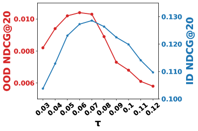
(a) MF+PopGo

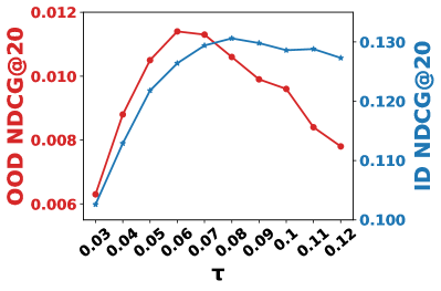
(b) LightGCN+PopGo

Figure 6. Temperature $\tau$ sensitivity analysis on Tencent.

4.4.2. Impact of Shortcut Model

To better understand the role of the shortcut model, we compare PopGo with a variant, PopGo-S that disables the shortcut model.

• Ablation Study. Table 5 shows that removing the shortcut model causes a huge performance drop on both ID and OOD tests. This verifies the rationality and effectiveness of the shortcut model.

• Correlation Analysis. With the shortcut loss in Equation (8), we calculate its Pearson correlation with the loss using the debiased prediction $\alpha_{ui}$ and the loss using shortcut-involved prediction $\alpha_{ui}\cdot\beta^{*}_{ui}$. Figure 7 displays that the correlation between $\mathbf{\mathop{\mathcal{L}}}_{b}$ and $\alpha_{ui}$-loss is smaller than that between $\mathbf{\mathop{\mathcal{L}}}_{b}$ and $\alpha_{ui}\cdot\beta^{*}_{ui}$-loss. It verifies that $\alpha_{ui}$ holds less popularity-relevant information, thus illustrating that PopGo indeed is effective at reducing the popularity bias.

• Visualizations of Representations. In Figure 8, we visualize the item representations learned by MF, MF+PopGo-S, and MF+PopGo on Amazon-Book via t-SNE (Van der Maaten and Hinton, 2008). We find that: (1) The item representations of MF are chaotically distributed and difficult to distinguish, which indicates that MF focuses more on popular shortcuts, rather than preference-relevant features, which is consistent with DICE (Zheng et al., 2021); (2) From MF+PopGo-S to MF+PopGo, the representations present a clearer boundary, which are well scattered based on item popularity rather than chaotically distributed. This justifies that PopGo can learn high-quality representations for both popular and unpopular items, revealing why PopGo could achieve significant improvements in both ID and OOD settings. To sum up, we can confirm the impact of PopGo’s shortcut model on improving the representation ability and generalization of CF models.

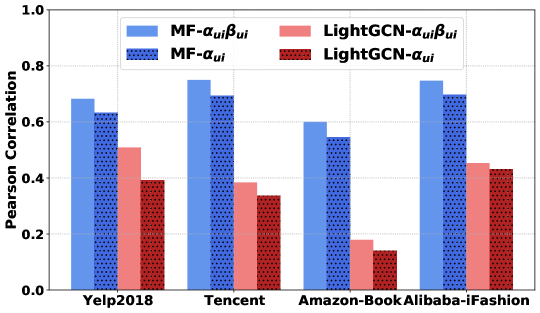
Figure 7. Correlation analysis on four datasets with both MF and LightGCN as the target models. Light color represents the correlation between the element-wise loss of dibiased models using $\alpha_{ui}$ as prediction and the shortcut model. Dark color denotes the correlation between the loss using masked prediction $\alpha_{ui}\cdot\beta_{ui}$ and the shortcut model.

5. Related Work

Existing debiasing strategies in CF roughly fall into five groups.

Inverse Propensity Score (IPS) methods (Schnabel et al., 2016; Joachims et al., 2018; Bottou et al., 2013; Gruson et al., 2019; Saito et al., 2020; Liang et al., 2016; Chen et al., 2021; Ding et al., 2022; Wang et al., 2019a) view the item popularity in the training set as the propensity score and exploit its inverse to re-weight loss of each instance. Hence, popular items are imposed lower weights, while the importance of long-tail items is boosted. However, (Schnabel et al., 2016; Joachims et al., 2018) suffer from the severe fluctuation of propensity score estimation due to their high variance of re-weighted loss. (Gruson et al., 2019; Bottou et al., 2013) further employ normalization or smoothing penalty to attain more stable output. Although IPS variants guarantee low bias, they use item frequency as a one-dimensional propensity score to capture only item-side popularity bias. This makes them fail to identify the actual interaction-wise and target model-related popularity bias. Recently, AutoDebias  (Chen et al., 2021) leverages a small set of uniform data to learn debiasing parameters. BRD  (Ding et al., 2022) obtains the boundary of the true propensity score before optimizing the model with adversarial learning. DR  (Wang et al., 2019a) proposes a doubly robust estimator to correct the deviations of errors inversely weighted with propensities.

Domain adaption methods (Bonner and Vasile, 2018; Liu et al., 2020; Chen et al., 2020b) utilize a small part of unbiased data as the target domain to guide the debiasing model training on biased source data. For example, CausE (Bonner and Vasile, 2018) forces the two representations learned from unbiased and biased data similar to each other. The recently proposed KDCRec (Liu et al., 2020) leverages knowledge distillation to transfer the knowledge obtained from biased data to the model of unbiased data. However, the decomposition of training data leads to two limitations - the debiased training set is often relatively small, and domain-specific information may lose. Thus, these drawbacks further result in a downgrade performance.

Causal embedding methods (Zheng et al., 2021; Wei et al., 2021; Wang et al., 2021; Zhang et al., 2021b; Xu et al., 2021; Gupta et al., 2021; Liu et al., 2020), getting inspiration from the recent success of causal inference, specify the role of popularity bias in assumed causal graphs and mitigate the bias effect on the prediction. DICE (Zheng et al., 2021) learned disentangled interest and conformity representations by training cause-specific data. MACR (Wei et al., 2021) performs multi-task learning to achieve the contribution of each cause and perform counterfactual inference to remove the popularity bias. CauSeR (Gupta et al., 2021) uses a holistic view to capture popularity biases in data generation as well as training stages. Using a systematic causal view of reducing popularity bias in CF, these causal embedding debiasing methods achieve state-of-the-art performance. However, despite the great success, Many of them assume the test distribution is known in advance and leverage this prior to adjusting the key hyperparameters.

Regularization-based methods (Chen et al., 2020b; Abdollahpouri et al., 2017; Boratto et al., 2021; Zhu et al., 2021) regularize the correlations of predicted scores and item popularity, so as to control the trade-off between recommendation accuracy and coverage. The major difference among these regularization methods is the design of penalty terms. For example, to measure the lack of fairness, ALS+Reg (Abdollahpouri et al., 2017) introduces an intra-list binary unfairness penalty; to achieve the distribution alignment, ESAM (Chen et al., 2020b) builds the penalty upon the correlation between high-level attributes of items; Reg (Zhu et al., 2021) decouples the item popularity with the predictive preferences; more recently, SAM+REG (Boratto et al., 2021) regulates the biased correlation between user-item relevance and item popularity; Nonetheless, most of them sacrifice overall accuracy to promote the ranking of tail items.

Generalized methods (Zhang et al., 2022, 2023b; Chen et al., 2022; Wen et al., 2022; Zhang et al., 2021a; Wang et al., 2022b; He et al., 2022; Wang et al., 2022a) aim to learn invariant representations against popularity bias and achieve stability and generalization ability. s-DRO  (Wen et al., 2022) adopts Distributionally Robust Optimization (DRO) framework, CD²AN  (Chen et al., 2022) disentangles item property representations from popularity under co-training networks. CausPref  (He et al., 2022) utilizes a differentiable structure learner in order to learn invariant and causal user preference. COR (Wang et al., 2022b) formulates feature shift as an intervention and performs counterfactual inference to mitigate the effect of out-of-date interactions. BC Loss (Zhang et al., 2022) incorporates popularity bias-aware margins to achieve better generalization ability. InvCF (Zhang et al., 2023b) discovers disentangled representations that faithfully reveal the latent preference and popularity semantics.

Our proposed PopGo also shares similarities with a recently emergent category of self-supervised learning (SSL) based Collaborative Filtering (CF) methods (Wu et al., 2021; Zhang et al., 2023a; Tian et al., 2022; Zhou et al., 2023). SSL-based CF methods aspire to boost representation learning in recommendation systems by utilizing the principle of contrastive learning. These methods frequently adopt the variant of softmax loss as their objective function.

6. Conclusion and Future work

In this paper, we proposed a simple yet effective debiasing strategy in CF, PopGo, which identifies the interaction-wise popularity shortcut degree by utilizing a shortcut model. Without any assumption or prior knowledge on the OOD test, PopGo achieves both ODD generalization and ID performance with high-quality debiased representations. Furthermore, we justify the rationality of PopGo from two theoretical perspectives: (1) from the perspective of causal inference, PopGo learns the total direct effect of user-item interactions on the prediction, while excluding the pure popularity effect; (2) from the perspective of information theory, PopGo intends to maximize the conditional mutual information between the interaction and prediction, conditioning on the popularity. Extensive experiments showcase that PopGo endows the CF models with better generalization.

PopGo primarily targets the reduction of popularity bias. An interesting avenue for future work would be to expand PopGo’s capabilities to mitigate multiple biases in CF, such as exposure and selection bias. It could even tackle more challenging scenarios, like the general debiasing in recommender systems. In addition, we aim to delve deeper into the generalization of recommender models, potentially providing theoretical evidence for performance improvement in out-of-distribution settings.

- (1)
- Abdollahpouri et al. (2017) Himan Abdollahpouri, Robin Burke, and Bamshad Mobasher. 2017. Controlling Popularity Bias in Learning-to-Rank Recommendation. In RecSys. 42–46.
- Abdollahpouri et al. (2019) Himan Abdollahpouri, Masoud Mansoury, Robin Burke, and Bamshad Mobasher. 2019. The Unfairness of Popularity Bias in Recommendation. In RMSE@RecSys (CEUR Workshop Proceedings, Vol. 2440).
- Bell et al. (2008) Robert M Bell, Yehuda Koren, and Chris Volinsky. 2008. The bellkor 2008 solution to the netflix prize. Statistics Research Department at AT&T Research 1, 1 (2008).
- Bellogín et al. (2017) Alejandro Bellogín, Pablo Castells, and Iván Cantador. 2017. Statistical biases in Information Retrieval metrics for recommender systems. Inf. Retr. J. 20, 6 (2017), 606–634.
- Bonner and Vasile (2018) Stephen Bonner and Flavian Vasile. 2018. Causal embeddings for recommendation. In RecSys. 104–112.
- Boratto et al. (2021) Ludovico Boratto, Gianni Fenu, and Mirko Marras. 2021. Connecting user and item perspectives in popularity debiasing for collaborative recommendation. Inf. Process. Manag. 58, 1 (2021), 102387.
- Bottou et al. (2013) Léon Bottou, Jonas Peters, Joaquin Quiñonero Candela, Denis Xavier Charles, Max Chickering, Elon Portugaly, Dipankar Ray, Patrice Y. Simard, and Ed Snelson. 2013. Counterfactual reasoning and learning systems: the example of computational advertising. J. Mach. Learn. Res. 14, 1 (2013), 3207–3260.
- Cañamares and Castells (2018) Rocío Cañamares and Pablo Castells. 2018. Should I Follow the Crowd?: A Probabilistic Analysis of the Effectiveness of Popularity in Recommender Systems. In SIGIR. 415–424.
- Chen et al. (2021) Jiawei Chen, Hande Dong, Yang Qiu, Xiangnan He, Xin Xin, Liang Chen, Guli Lin, and Keping Yang. 2021. AutoDebias: Learning to Debias for Recommendation. In SIGIR. ACM, 21–30.
- Chen et al. (2020a) Jiawei Chen, Hande Dong, Xiang Wang, Fuli Feng, Meng Wang, and Xiangnan He. 2020a. Bias and Debias in Recommender System: A Survey and Future Directions. CoRR abs/2010.03240 (2020).
- Chen et al. (2019) Wen Chen, Pipei Huang, Jiaming Xu, Xin Guo, Cheng Guo, Fei Sun, Chao Li, Andreas Pfadler, Huan Zhao, and Binqiang Zhao. 2019. POG: Personalized Outfit Generation for Fashion Recommendation at Alibaba iFashion. In KDD. 2662–2670.
- Chen et al. (2022) Zhihong Chen, Jiawei Wu, Chenliang Li, Jingxu Chen, Rong Xiao, and Binqiang Zhao. 2022. Co-training Disentangled Domain Adaptation Network for Leveraging Popularity Bias in Recommenders. In SIGIR.
- Chen et al. (2020b) Zhihong Chen, Rong Xiao, Chenliang Li, Gangfeng Ye, Haochuan Sun, and Hongbo Deng. 2020b. ESAM: Discriminative Domain Adaptation with Non-Displayed Items to Improve Long-Tail Performance. In SIGIR. 579–588.
- Ding et al. (2022) Sihao Ding, Peng Wu, Fuli Feng, Yitong Wang, Xiangnan He, Yong Liao, and Yongdong Zhang. 2022. Addressing Unmeasured Confounder for Recommendation with Sensitivity Analysis. In KDD.
- Ebesu et al. (2018) Travis Ebesu, Bin Shen, and Yi Fang. 2018. Collaborative Memory Network for Recommendation Systems. In SIGIR. 515–524.
- Gruson et al. (2019) Alois Gruson, Praveen Chandar, Christophe Charbuillet, James McInerney, Samantha Hansen, Damien Tardieu, and Ben Carterette. 2019. Offline Evaluation to Make Decisions About Playlist Recommendation Algorithms. In WSDM. 420–428.
- Gupta et al. (2021) Priyanka Gupta, Ankit Sharma, Pankaj Malhotra, Lovekesh Vig, and Gautam Shroff. 2021. CauSeR: Causal Session-based Recommendations for Handling Popularity Bias. In CIKM.
- He and McAuley (2016) Ruining He and Julian J. McAuley. 2016. Ups and Downs: Modeling the Visual Evolution of Fashion Trends with One-Class Collaborative Filtering. In WWW. ACM, 507–517.
- He et al. (2020) Xiangnan He, Kuan Deng, Xiang Wang, Yan Li, Yong-Dong Zhang, and Meng Wang. 2020. LightGCN: Simplifying and Powering Graph Convolution Network for Recommendation. In SIGIR. 639–648.
- He et al. (2017) Xiangnan He, Lizi Liao, Hanwang Zhang, Liqiang Nie, Xia Hu, and Tat-Seng Chua. 2017. Neural Collaborative Filtering. In WWW. 173–182.
- He et al. (2022) Yue He, Zimu Wang, Peng Cui, Hao Zou, Yafeng Zhang, Qiang Cui, and Yong Jiang. 2022. CausPref: Causal Preference Learning for Out-of-Distribution Recommendation. In WWW.
- Jannach et al. (2015) Dietmar Jannach, Lukas Lerche, Iman Kamehkhosh, and Michael Jugovac. 2015. What recommenders recommend: an analysis of recommendation biases and possible countermeasures. User Model. User Adapt. Interact. 25, 5 (2015), 427–491.
- Ji et al. (2020) Yitong Ji, Aixin Sun, Jie Zhang, and Chenliang Li. 2020. A Re-visit of the Popularity Baseline in Recommender Systems. In SIGIR. 1749–1752.
- Joachims et al. (2018) Thorsten Joachims, Adith Swaminathan, and Tobias Schnabel. 2018. Unbiased Learning-to-Rank with Biased Feedback. In IJCAI. ijcai.org, 5284–5288.
- Kabbur et al. (2013) Santosh Kabbur, Xia Ning, and George Karypis. 2013. FISM: factored item similarity models for top-N recommender systems. In KDD. 659–667.
- Kim et al. (2022) Minseok Kim, Jinoh Oh, Jaeyoung Do, and Sungjin Lee. 2022. Debiasing Neighbor Aggregation for Graph Neural Network in Recommender Systems. In CIKM.
- Kingma and Ba (2015) Diederik P. Kingma and Jimmy Ba. 2015. Adam: A Method for Stochastic Optimization. In ICLR (Poster).
- Koren (2008) Yehuda Koren. 2008. Factorization meets the neighborhood: a multifaceted collaborative filtering model. In SIGKDD. 426–434.
- Krichene and Rendle (2020) Walid Krichene and Steffen Rendle. 2020. On Sampled Metrics for Item Recommendation. In KDD. 1748–1757.
- Kullback (1997) Solomon Kullback. 1997. Information theory and statistics. Courier Corporation.
- Liang et al. (2016) Dawen Liang, Laurent Charlin, and David M Blei. 2016. Causal inference for recommendation. In Causation: Foundation to Application, Workshop at UAI. AUAI.
- Liang et al. (2018) Dawen Liang, Rahul G. Krishnan, Matthew D. Hoffman, and Tony Jebara. 2018. Variational Autoencoders for Collaborative Filtering. In WWW. 689–698.
- Liu et al. (2020) Dugang Liu, Pengxiang Cheng, Zhenhua Dong, Xiuqiang He, Weike Pan, and Zhong Ming. 2020. A General Knowledge Distillation Framework for Counterfactual Recommendation via Uniform Data. In SIGIR. 831–840.
- Mao et al. (2021) Kelong Mao, Jieming Zhu, Xi Xiao, Biao Lu, Zhaowei Wang, and Xiuqiang He. 2021. UltraGCN: Ultra Simplification of Graph Convolutional Networks for Recommendation. In CIKM.
- Marlin and Zemel (2009) Benjamin M. Marlin and Richard S. Zemel. 2009. Collaborative prediction and ranking with non-random missing data. In RecSys.
- Niu and Zhang (2021) Yulei Niu and Hanwang Zhang. 2021. Introspective Distillation for Robust Question Answering. In NeurIPS.
- Park and Tuzhilin (2008) Yoon-Joo Park and Alexander Tuzhilin. 2008. The long tail of recommender systems and how to leverage it. In RecSys. ACM, 11–18.
- Pearl (2000) Judea Pearl. 2000. Causality: Models, Reasoning, and Inference.
- Pearl et al. (2016) Judea Pearl, Madelyn Glymour, and Nicholas P Jewell. 2016. Causal inference in statistics: A primer. John Wiley & Sons.
- Poole et al. (2019) Ben Poole, Sherjil Ozair, Aäron van den Oord, Alex Alemi, and George Tucker. 2019. On Variational Bounds of Mutual Information. In ICML (Proceedings of Machine Learning Research, Vol. 97). 5171–5180.
- Rendle (2021) Steffen Rendle. 2021. Item Recommendation from Implicit Feedback. CoRR abs/2101.08769 (2021).
- Rendle et al. (2012) Steffen Rendle, Christoph Freudenthaler, Zeno Gantner, and Lars Schmidt-Thieme. 2012. BPR: Bayesian Personalized Ranking from Implicit Feedback. CoRR abs/1205.2618 (2012).
- Rendle et al. (2020) Steffen Rendle, Walid Krichene, Li Zhang, and John R. Anderson. 2020. Neural Collaborative Filtering vs. Matrix Factorization Revisited. In RecSys. 240–248.
- Robins and Greenland (1992) James M Robins and Sander Greenland. 1992. Identifiability and exchangeability for direct and indirect effects. Epidemiology (1992), 143–155.
- Saito et al. (2020) Yuta Saito, Suguru Yaginuma, Yuta Nishino, Hayato Sakata, and Kazuhide Nakata. 2020. Unbiased Recommender Learning from Missing-Not-At-Random Implicit Feedback. In WSDM. 501–509.
- Schnabel et al. (2016) Tobias Schnabel, Adith Swaminathan, Ashudeep Singh, Navin Chandak, and Thorsten Joachims. 2016. Recommendations as Treatments: Debiasing Learning and Evaluation. In ICML. 1670–1679.
- Song et al. (2019) Weiping Song, Zhiping Xiao, Yifan Wang, Laurent Charlin, Ming Zhang, and Jian Tang. 2019. Session-Based Social Recommendation via Dynamic Graph Attention Networks. In WSDM. ACM, 555–563.
- Teney et al. (2020) Damien Teney, Ehsan Abbasnejad, Kushal Kafle, Robik Shrestha, Christopher Kanan, and Anton van den Hengel. 2020. On the Value of Out-of-Distribution Testing: An Example of Goodhart’s Law. In NeurIPS.
- Tian et al. (2022) Changxin Tian, Yuexiang Xie, Yaliang Li, Nan Yang, and Wayne Xin Zhao. 2022. Learning to Denoise Unreliable Interactions for Graph Collaborative Filtering. In SIGIR.
- Van der Maaten and Hinton (2008) Laurens Van der Maaten and Geoffrey Hinton. 2008. Visualizing data using t-SNE. Journal of machine learning research 9, 11 (2008).
- VanderWeele (2013) Tyler J VanderWeele. 2013. A three-way decomposition of a total effect into direct, indirect, and interactive effects. Epidemiology (Cambridge, Mass.) 24, 2 (2013), 224.
- Wang et al. (2019b) Hongwei Wang, Fuzheng Zhang, Mengdi Zhang, Jure Leskovec, Miao Zhao, Wenjie Li, and Zhongyuan Wang. 2019b. Knowledge-aware Graph Neural Networks with Label Smoothness Regularization for Recommender Systems. In KDD. 968–977.
- Wang et al. (2021) Wenjie Wang, Fuli Feng, Xiangnan He, Xiang Wang, and Tat-Seng Chua. 2021. Deconfounded Recommendation for Alleviating Bias Amplification. In KDD. ACM, 1717–1725.
- Wang et al. (2022b) Wenjie Wang, Xinyu Lin, Fuli Feng, Xiangnan He, Min Lin, and Tat-Seng Chua. 2022b. Causal Representation Learning for Out-of-Distribution Recommendation. In WWW.
- Wang et al. (2019a) Xiaojie Wang, Rui Zhang, Yu Sun, and Jianzhong Qi. 2019a. Doubly Robust Joint Learning for Recommendation on Data Missing Not at Random. In ICML.
- Wang et al. (2022a) Zimu Wang, Yue He, Jiashuo Liu, Wenchao Zou, Philip S. Yu, and Peng Cui. 2022a. Invariant Preference Learning for General Debiasing in Recommendation. In KDD.
- Wang et al. (2020) Ze Wang, Guangyan Lin, Huobin Tan, Qinghong Chen, and Xiyang Liu. 2020. CKAN: Collaborative Knowledge-aware Attentive Network for Recommender Systems. In SIGIR. 219–228.
- Wei et al. (2021) Tianxin Wei, Fuli Feng, Jiawei Chen, Ziwei Wu, Jinfeng Yi, and Xiangnan He. 2021. Model-Agnostic Counterfactual Reasoning for Eliminating Popularity Bias in Recommender System. In KDD. 1791–1800.
- Wen et al. (2022) Hongyi Wen, Xinyang Yi, Tiansheng Yao, Jiaxi Tang, Lichan Hong, and Ed H Chi. 2022. Distributionally-robust Recommendations for Improving Worst-case User Experience. In WWW.
- Wiles et al. (2022) Olivia Wiles, Sven Gowal, Florian Stimberg, Sylvestre-Alvise Rebuffi, Ira Ktena, Krishnamurthy Dvijotham, and Ali Taylan Cemgil. 2022. A Fine-Grained Analysis on Distribution Shift. In ICLR.
- Wu et al. (2021) Jiancan Wu, Xiang Wang, Fuli Feng, Xiangnan He, Liang Chen, Jianxun Lian, and Xing Xie. 2021. Self-supervised Graph Learning for Recommendation. In SIGIR. ACM, 726–735.
- Xu et al. (2021) Shuyuan Xu, Juntao Tan, Shelby Heinecke, Jia Li, and Yongfeng Zhang. 2021. Deconfounded Causal Collaborative Filtering. CoRR abs/2110.07122.
- Ye et al. (2022) Nanyang Ye, Kaican Li, Haoyue Bai, Runpeng Yu, Lanqing Hong, Fengwei Zhou, Zhenguo Li, and Jun Zhu. 2022. OoD-Bench: Quantifying and Understanding Two Dimensions of Out-of-Distribution Generalization. In CVPR. 7937–7948.
- Ying et al. (2018) Rex Ying, Ruining He, Kaifeng Chen, Pong Eksombatchai, William L. Hamilton, and Jure Leskovec. 2018. Graph Convolutional Neural Networks for Web-Scale Recommender Systems. In KDD. 974–983.
- Yuan et al. (2020) Fajie Yuan, Xiangnan He, Haochuan Jiang, Guibing Guo, Jian Xiong, Zhezhao Xu, and Yilin Xiong. 2020. Future Data Helps Training: Modeling Future Contexts for Session-based Recommendation. In Proceedings of The Web Conference 2020. 303–313.
- Zhang et al. (2022) An Zhang, Wenchang Ma, Xiang Wang, and Tat seng Chua. 2022. Incorporating Bias-aware Margins into Contrastive Loss for Collaborative Filtering. In NeurIPS.
- Zhang et al. (2023a) An Zhang, Leheng Sheng, Zhibo Cai, Xiang Wang, and Tat seng Chua. 2023a. Empowering Collaborative Filtering with Principled Adversarial Contrastive Loss. In NeurIPS.
- Zhang et al. (2023b) An Zhang, Jingnan Zheng, Xiang Wang, Yancheng Yuan, and Tat seng Chua. 2023b. Invariant Collaborative Filtering to Popularity Distribution Shift. In WWW.
- Zhang et al. (2021a) Yin Zhang, Derek Zhiyuan Cheng, Tiansheng Yao, Xinyang Yi, Lichan Hong, and Ed H. Chi. 2021a. A Model of Two Tales: Dual Transfer Learning Framework for Improved Long-tail Item Recommendation. In WWW.
- Zhang et al. (2021b) Yang Zhang, Fuli Feng, Xiangnan He, Tianxin Wei, Chonggang Song, Guohui Ling, and Yongdong Zhang. 2021b. Causal Intervention for Leveraging Popularity Bias in Recommendation. In SIGIR. 11–20.
- Zheng et al. (2021) Yu Zheng, Chen Gao, Xiang Li, Xiangnan He, Yong Li, and Depeng Jin. 2021. Disentangling User Interest and Conformity for Recommendation with Causal Embedding. In WWW. 2980–2991.
- Zhou et al. (2023) Huachi Zhou, Hao Chen, Junnan Dong, Daochen Zha, Chuang Zhou, and Xiao Huang. 2023. Adaptive Popularity Debiasing Aggregator for Graph Collaborative Filtering. In SIGIR.
- Zhu et al. (2021) Ziwei Zhu, Yun He, Xing Zhao, Yin Zhang, Jianling Wang, and James Caverlee. 2021. Popularity-Opportunity Bias in Collaborative Filtering. In WSDM. ACM, 85–93.
- Zhu et al. (2020) Ziwei Zhu, Jianling Wang, and James Caverlee. 2020. Measuring and Mitigating Item Under-Recommendation Bias in Personalized Ranking Systems. In SIGIR. ACM, 449–458.