Smart OMVI: Obfuscated Malware Variant Identification using a novel dataset

Abstract

Cybersecurity has become a significant issue in the digital era as a result of the growth in everyday computer use. Cybercriminals now engage in more than virus distribution and computer hacking. Cyberwarfare has developed as a result because it has become a threat to a nation’s survival. Malware analysis serves as the first line of defence against an attack and is a significant component of cybercrime. Every day, malware attacks target a large number of computer users, businesses, and governmental agencies, causing billions of dollars in losses. Malware may evade multiple AV software with a very minor, cunning tweak made by its designers, despite the fact that security experts have a variety of tools at their disposal to identify it. To address this challenge, a new dataset called the Obfuscated Malware Dataset (OMD) has been developed. This dataset comprises 40 distinct malware families having 21924 samples, and it incorporates obfuscation techniques that mimic the strategies employed by malware creators to make their malware variations different from the original samples. The purpose of this dataset is to provide a more realistic and representative environment for evaluating the effectiveness of malware analysis techniques. Different conventional machine learning algorithms including but not limited to Support Vector Machine (SVM), Random Forrest (RF), Extreme Gradient Boosting (XGBOOST) etc are applied and contrasted. The results demonstrated that XGBoost outperformed the other algorithms, achieving an accuracy of f 82%, precision of 88%, recall of 80%, and an F1-Score of 83%.

Keywords Antivirus  $\cdot$ OMD  $\cdot$ Malware  $\cdot$ Obfuscation, Identification  $\cdot$ Variants  $\cdot$ Malware classification

1 Introduction

Malicious software shortened to malware, is a piece of software made with the intention of breaking into and causing harm to computers without the user’s knowledge. The word "malware" refers to a broad category of destructive software; some of the most popular varieties are listed in table 1. Software malware may come in a variety of shapes and sizes. Desktops, servers, mobile phones, printers, and programmable electrical circuits are just a few possible deployment platforms. Sophisticated assaults have proven that data may be taken using well-written malware that only exists in system memory and leaves no trace in the form of permanent data. Information security safeguards like desktop firewalls and anti-virus software have been reported to be disabled by malware. Some are even capable of compromising audit, authentication, and authorisation processes.

Table 1: Common Malware Types

Type	Description
Adware Gao et al. (2019)	They display unwanted advertisements on a computer or mobile device resulting in slowdowm. It often gets installed alongside other software without the user’s knowledge or consent, and can collect data about the user’s browsing habits.
Bot	Automated programs that can perform various tasks, including useful and malicious ones, on the internet. Botnets, networks of infected computers controlled by a botmaster, can be used to carry out large-scale attacks.
Bug	Flaws or errors in software code that can cause unexpected behavior ranging from minor glitches to serious security vulnerabilities that can be exploited by attackers to gain unauthorized access or cause system crashes.
Ransomware	A type of malware that encrypts a victim’s files and demands payment in exchange for the decryption key. These attacks can be devastating for individuals and organizations, causing loss of data and significant financial costs.
Rootkit	It allows an attacker to gain root-level access to a computer system which can be used to hide other malware, steal sensitive data, or control the system remotely. Usually, rootkits are very difficult to detect and remove, often requiring specialized tools and expertise.
Spyware	A type of malicious software designed to gather sensitive information such as personal information including but not limited to passwords, credit card numbers, and browsing history from a computer or mobile device
Trojan Horse	Disguised as a legitimate program, but once installed, can give unauthorized access to a computer system or steal sensitive data. A variety of harmful actions, such as deleting files, stealing passwords, or opening up a backdoor for remote access can be performed by them.
Virus	Self-replication and fast spread are the identifying features of a virus. These can cause a range of damages, from data loss to system crashes, and can be difficult to remove once activated.
Worms	These can cause harm by overloading systems, stealing information, or carrying out other malicious actions. Some famous examples of worms include Code Red, Conficker, and WannaCry.
Scareware	A type of malware that tries to trick users into thinking their computer is infected with a virus or other threat. These typically displays fake pop-ups or alerts urging the user to purchase bogus security software or services which can be harmful if users fall for the scam and download the fake software, which may contain actual malware.
Fileless Malware	A type of malware that operates entirely in a device’s memory or system registry, leaving little to no trace on disk and thus, is harder to detect and remove than traditional malware because it doesn’t leave the same types of artifacts. Examples of fileless malware include PowerShell-based attacks and memory-based exploits.
Keyloggers	These capture keystrokes typed on a device’s keyboard, potentially allowing the attacker to steal sensitive information like passwords or credit card numbers. They can be either software or hardware-based, with the latter being more difficult to detect. Some even have the ability to capture screenshots or record audio or video from the device.
Wiper	A type of malware that is designed to destroy or wipe out data on a device or network. These attacks can be devastating, as they can render a system completely unusable and may be difficult or impossible to recover from. Some notable examples of wiper malware include Shamoon, NotPetya, and OlympicDestroyer.

Even when a compromised machine is rebooted, startup files have been set to preserve persistence. When run, advanced malware may duplicate itself or remain dormant until called upon by its command features to extract data or delete files. Four operational characteristics often serve to characterise a particular piece of malware:

1. Propagation: The method through which malware spreads across several systems.

2. Infection: The malware’s method of installation and its capacity to withstand cleanup efforts after being set up.

3. Self-Defense: The technique utilised to obfuscate its existence and thwart examination.

4. Capabilities: Functions accessible by malware operator.

These might also be referred to as anti-reversing capabilities.

Table 2: List of Abbreviations

Abbreviations	Full Form
OMD	Obfucated Malware Datase
RNN	Recurrent Neural Network
PUA	Potentially Unwanted Applications
CCV	Card Code Verification
ASM	Assembly language
NOP	No Operation

1.1 Different Families of Malware

Malware are categorized into different families on the basis of their behavior and type of damage done to host machine.

1.2 Criminal Steps of Malware

Malware are diverse in their kind and activity, attacking different types of information in order to cause problems for the user.

1. Intelligence gathering: A criminal searches the target for weak spots in order to prepare an assault.

2. Preparation: A criminal develops, tweaks, or somehow acquires malware to meet the demands of an attack.

3. Distribution: The spread of malware takes place.

4. Compromise: Malware infects the system.

5. Demand: The power of malware is released.

6. Execution: Malware transfers data to the malware operator, a process known as exfiltration, which achieves the attack’s goal by transferring data from an information system without any type of consent.

Modern malware remediation is getting harder and harder to do for a variety of reasons. Malware that exploits the use zero-day vulnerabilities Kumar and Subbiah (2022); Barros et al. (2022) comes in a much wider range of forms. A vulnerability is described as "zero-day" if potential victims are unaware of it, in which case they have no time to prepare. Malware is now capable of taking on several forms thanks to polymorphic design. Malware that is polymorphic alters some aspects of itself with each infection. This modification may take the form of an unusable code update. This method avoids signature-based detection Botacin et al. (2022) methods since they frequently create a distinct signature from a file containing malware using a hash algorithm, meaning that any modification to the file would alter its signature. Moreover, because polymorphic Selamat and Ali (2022) malware has the ability to alter its own filename upon infection, standard signature-based methods of detection are hampered. As a result, to address this problem, a new dataset called the Obfucated Malware Dataset (OMD) is presented. The following are the overall contributions of this work:

1. A large malware dataset named Obfucated Malware Dataset (OMD) is generated by collecting malware data from different sources, combining them with two other datasets, namely, Malimg and Kaggle’s Microsoft Malware Classification Challenge (BIG 2015) Dataset and applying various obfuscation techniques resulting in 40 different families of malware. The final dataset contains 40 classes and 21924 samples.

2. In contrast to other datasets, all samples in OMD are obfuscated using different techniques resulting in a dataset that can mimic new or polymorphic malwares. Traditional machine learning techniques are applied on the dataset and results are compared and contrasted.

The rest of the paper is organized as follows. The next section highlights the related work in the field of malware classification. Section 3 explains our novel classification framework methodology, while section 4 discusses the experimental setup. Section 5 presents the result analysis and discussion of our work. Section 6 concludes the paper.

2 Related Work

Any software that is intentionally designed to disrupt a computer, server, client, or computer network, leak sensitive information, allow unauthorised access to data or systems, deny access to information, or inadvertently compromise user privacy and security on computers is known as malware, a combination of words malicious and software Brewer (2016); Tahir (2018).

Table 3: Stolen data prices

Data type	Price
CCV	$3.25
OS administrative login	$2.50
FTP exploit	$6.00
Full identity information	$5.00
Rich bank account credentials	$750.00
US passport information	$800.00
Router credentials	$12.50

Table 4: Cost of Malware and Crimeware

Theft Enabling Commodity	Price
Keystroke logger	$25 on average
Botnets	$100 to $200 per 1,000 infections, depending on location
Spamming email service	$.01 per 1,000 emails, reliability of more than 85% delivered
Shop admins (Credit Card databases)	$100 to $300
Credit Card numbers without CCV2	$1 to $3
Credit Card numbers with CCV2	$1.50 to $10.00, depending on the country
Socks accounts	$5 to $40/month
Sniffer dumps	$50 to $100/month
Western Union exploits	$300 to $1,000
Remote desktops	$5 to $8
Scam letters	$3 to $5

The underground market for stolen data is the chief reason of malware. In several forums, data hackers may resell their loot Menn (2010). Table 3 Geer and Conway (2009) contains examples of prices paid for various categories of stolen data. The money demanded for the stolen goods indicated in Table 3 drove the development of secondary malware marketplaces, which result in software tools that make malware more and more successful at facilitating information theft. In general, people utilise software to automate laborious and resource-intensive jobs, and malware authors are no different. Automating the transmission of malware and the data collection process lowers operating expenses while enabling criminals to conceal their operations. Systems for the distribution and operation of malware have gotten more and more modular. Crimeware Salloum et al. (2022); Wang et al. (2021) is a term used to describe software that has been found to have such malware support systems. The Zeus toolkit Grammatikakis et al. (2021) is a good illustration of crimeware. The Zeus virus first appeared in 2006, and the associated crimeware in 2007. Zeus’ crimeware takes use of its modular nature, so attackers may modify and deploy new capabilities relatively rapidly. An attacker may choose the features to be included in a "release" and a unique encryption key for data that has been captured using an intuitive graphical interface. Zeus crimeware has been used to produce more than 5,000 different versions of the Zeus software. Although numerous Zeus users have been identified and prosecuted with cybercrimes, the Zeus crimeware writers remain at large Kazi et al. (2022); Rose et al. (2022).

2.1 Detecttion and Classfication

For the purpose of classifying and detecting malware, both static and dynamic analysis approaches have been widely used. The development of machine learning has created a wide range of possibilities for analysis and forecasting for both malware analysis methods. Visual malware image-based categorization is a relatively new development in the field of malware analysis. The textural elements of the malware’s visual image file were discovered in 2011 by Nataraj et al. Nataraj et al. (2011) . These files are generated by translating the byte code of a portable executable (PE) binary file to the pixel value’s grey level. They used wavelet decomposition to obtain the textural characteristics from the malware picture. The K-nearest Neighbor machine learning algorithm is then used on these characteristics.

Gibert et al. (2019) suggested a simple design for a convolutional neural network made up of three convolutional blocks, one fully-connected block, and one output layer. ReLU activation, max-pooling, normalization, and a convolution operation made up each convolution block. The convolutional layers served as detection filters for certain features or patterns in the input, while the following fully-connected layers combined the learnt information to produce a particular target output. The effectiveness of their method was tested on the Microsoft Malware Classification Challenge Ronen et al. (2018) versus manually created feature extractors Kancherla and Mukkamala (2013); Ahmadi et al. (2016), and the findings show that deep learning architectures perform better at identifying malware represented as grayscale photos. Similar to this, Rezende et al. (2017) performed classification on the MalImg Nataraj et al. (2011) dataset using the ResNet-50 architecture with pretrained weights.

2.2 Notable Datasets

Malware datasets with coarse family labels are shown in Table 5. The MalImg, VX Heaven Qiao et al. (2016), Kaggle, and MalDozer Karbab et al. (2018) datasets’ collecting periods are unrecorded; publishing dates are taken as an upper limit for the period’s conclusion. Drebin’s Arp et al. (2014) labels appear to have been combined from those of 10 other antivirus programs, while the precise labelling process is unknown. The Microsoft Security Essentials program was used to label the MalImg dataset. The VX Heaven website was active from 1999 to 2012, and the malware in the collection is thought to be extremely old. The Kaspersky antivirus software was used to label the VX Heaven dataset. MalDozer’s labelling strategy was not made public, however family names imply that one antivirus was used. Family labels are not present in the initial EMBER Anderson and Roth (2018) dataset, but an extra 1,000,000 files—both harmful and benign—were made available in 2018. AVClass Sebastián et al. (2016) labels indicate that 485,000 of these files are malware samples. The Malpedia Plohmann et al. (2017) collection includes labels that were received from open-source reporting, and some malware samples were dumped and unpacked using human analysis. Other family designations, however, were generated automatically using tools like YARA rules and comparisons of unpacked files to known malware samples.

The bulk of files in the Malsign Kotzias et al. (2015) collection are not malicious programs but rather PUAs. Malsign reference labels were created by clustering characteristics that had been statically extracted. MaLabel has 115,157 samples, of which 46,157 are part of 11 major families and the rest 69,000 are a part of families with fewer than 1,000 samples. The dataset contains an unknown number of families in total. Microsoft provided a collection of 1.3 million malware samples, labelled using a combination of antivirus labelling and manual labelling, to the developers of the MtNet Huang and Stokes (2016) malware classifier.

Although there are some datasets that has a few obfuscated malware samples, no dataset is purely focused on obfuscated malware classification. Using malware reference datasets with these proprties may yield evaluation results that are biased or incorrect for newer malwares. There aren’t many prominent datasets that contain malware that targets other operating systems (including Linux, macOS, and iOS), but this research is outside the purview of our article.

Table 5: Notable Datasets

Name	Year	Samples	Family	Operating System	Labelling Methodology	Period of collection
MOTIF	2022	3,095	454	Windows	Threat Reports	Jan. 2016 - Jan. 2021
MalImg	2011	9,458	25	Windows	Single AV	July 2011 or earlier
Kaggle	2018	10,868	9	Windows	Susp. Single AV	Feb. 2015 or earlier
AMD	2017	24,553	71	Android	Cluster Labeling	2010 - 2016
MalDozer	2018	20,089	32	Android	Susp. Single AV	Mar. 2018 or earlier
EMBER	2018	485,000	3,226	Windows	AVClass	2018
MalGenome	2015	1,260	49	Android	Threat Reports	Aug. 2010 - Oct. 2011
Variant	2015	85	8	Windows	Threat Reports	Jan. 2014
Malheur Rieck	2006	3,133	24	Windows	AV Majority Vote	2006 - 2009
Drebin	2010	5,560	179	Android	AV-based	Aug. 2010 - Oct. 2012
VX Heaven	2016	271,092	137	Windows	Single AV	2012
Malicia	2012	11,363	55	Windows	Cluster Labeling	Mar. 2012 - Mar. 2013
Malpedia	2017	5,862	2,165	Both	Hybrid	2017- ongoing
Malsign	2015	142,513	Unknown	Windows	Cluster labeling	2012- 2014
MaLabel	2015	115,157	>80	Windows	AV Majority Vote	Apr. 2015
MtNet	2016	1,300,000	98	Windows	Hybrid	Jun. 2016

3 Methodology

Table 6: Three datasets used to create OMD

Dataset Name	Number of Families	Number of Samples
Malimg	25	9339
Kaggle’s Microsoft Malware Classification Challenge (BIG 2015)	9	10868
TinyOMD	6	489
Total	40	21924

Table 7: Malimg Dataset

S.No.	Family	Family Name	Number of samples
$1$	Dailer	Adialer.C	122
$2$	Backdoor	Agent.FYI	116
$3$	Worm	Allaple.A	2949
$4$	Worm	Allaple.L	1591
$5$	Trojan	Alueron.gen!J	198
$6$	Worm:AutoIT	Autorun.K	106
$7$	Trojan	C2lop.gen!G	200
$8$	Trojan	C2lop.p	146
$9$	Dailer	Diaplaform.B	177
$10$	TrojanDownloader	Dontovo.A	162
$11$	Rogue	Fakerean	381
$12$	Dailer	Instantaccess	431
$13$	PWS	Lolyda.AA1	213
$14$	PWS	Lolyda.AA2	184
$15$	PWS	Lolyda.AA3	123
$16$	PWS	Lolyda.AT	159
$17$	Trojan	Malex.gen!J	136
$18$	TrojanDownloader	Obfuscated.AD	142
$19$	Backdoor	Rbot!gen	158
$20$	Trojan	Skintrim.N	80
$21$	TrojanDownloader	Swizzor.gen!E	128
$22$	TrojanDownloader	Swizzor.gen!I	132
$23$	Worm	VB.AT	408
$24$	TrojanDownloader	Wintrim.BX	97
$25$	Worm	Yuner.A	800
	Total		9339

Table 8: Obfuscated Malware Dataset (OMD))

S.No.	Family	Family Name	Number of samples
$1$	Backdoor	Gatak	1013
$2$	Backdoor	Kelihos_ver1	398
$3$	Backdoor	Kelihos_ver3	2493
$4$	Adware	Lollipop	2476
$5$	Any Obfuscated Malware	Obfuscator.ACY	1228
$6$	Worm	Ramnit	1541
$7$	Backdoor	Simda	42
$8$	TrojanDownloader	Tracur	751
$9$	Trojan	Vundo	475
	Total		10868

3.1 Dataset Generation

Dataset is one of the most important things in machine and deep learning. An appropriate dataset was required that mimics the polymorphism of modern malware families, hence, a dataset named as OMD shown in fig. 4 is created using three smaller datasets given in table 6. First dataset is Malimg Dataset represented in table 7 that comprises of 9339 malware samples which were classified into 25 malware families. This dataset contains grey-scale images formed from malware binaries. A 2D matrix was generated from these malware binaries and then represented as grey-scale images. Second dataset was Kaggle Malware Classification challenge 2015 dataset represented in table 8 containing 10868 malware samples that contain 9 different malware families. This dataset doesn’t contain malware samples in the form of grey-scale images, instead, it has ASM and Byte type malware sample files. ASM files were taken, different obfuscations were applied, and then these files were converted to grey-scale in order to add them to the dataset. Third dataset 10 was generated using malware samples collected from different sources and manually labelling them with the help of VirusTotal. Similar obfuscation techniques were also applied on this dataset. It was named as Tiny Obfuscated Malware Dataset (TinyOMD) shown in figure 1 and has 489 samples representing 6 classes given in Table 10. So, to Conclude three dataset namely Malimg, Kaggle Malware Classification challenge 2015 dataset and TinyOMD amounting to a total of 20696 and 40 classes given in table 6. Next step is Obfuscation, multiple techniques are applied for data obfuscation which explained in obfuscation section.

3.2 Obfuscation

Obfuscation is applied by help of two obfuscation blocks each containing six different obfuscation techniques, furthermore, encryption is applied to 20% of malware samples at random and combined with the reaming 80% to formulate the Obfuscated Malware Classification Dataset.

3.2.1 Obfuscation Block-I

Six obfuscation techniques applied in the first block were Dead-Code Insertion, Subroutine Reordering, Register Reassignment, XOR-Operation, Instruction Substitution and Code Transposition. This block is applied on ASM sample files in Kaggle’s Microsoft Classification 2015 Dataset and the newly created Tiny Obfuscated Malware Dataset (TinyOMD). All these techniques change malware source code thus resulting in change of signature without having any impact on its functionality. Dead-Code Insertion also known as NOp-Insertion is an instruction that itself doesn’t result in any sort of change in the functionally of the malware but is used to change its signature. It is commonly known as dead obfuscation. Code Transposition also known as Jump instruction transfers the program sequence to the memory address given in the operand based on the specified flag. This results in complex and difficult to understand code obfuscation. In Register Reassignment, extra lines of code are added, again resulting in change in malware signature.

3.2.2 Obfuscation Block-II

Six different obfuscation techniques were also applied in the second obfuscation block, namely, masking, in-painting, blurring, warping, scrambling, and tokenization. This block is applied on image sample files in all three sub-datasets including Malimg dataset, Kaggle’s Microsoft Classification 2015 Dataset and the newly created Tiny Obfuscated Malware Dataset (TinyOMD). These techniques make malware detection even more difficult. Furthermore, around 10% malware samples were taken at random from overall dataset, encrypted and added back to the dataset.

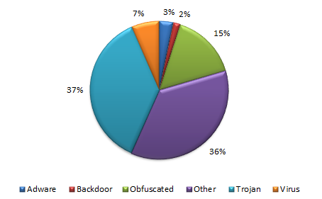
(a)

Figure 1: TinyOMD Classes with percentage of samples.

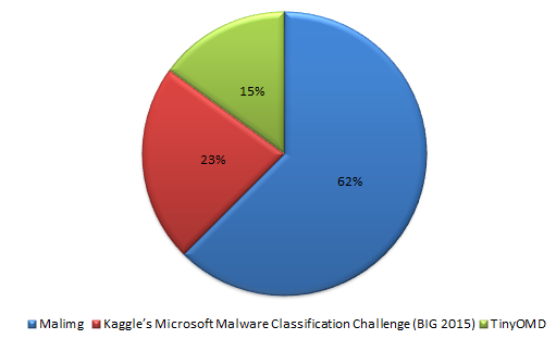
(a)

Figure 2: Percentage of each dataset samples in OMD

(a)

Figure 3: Major malware families sample count in OMD

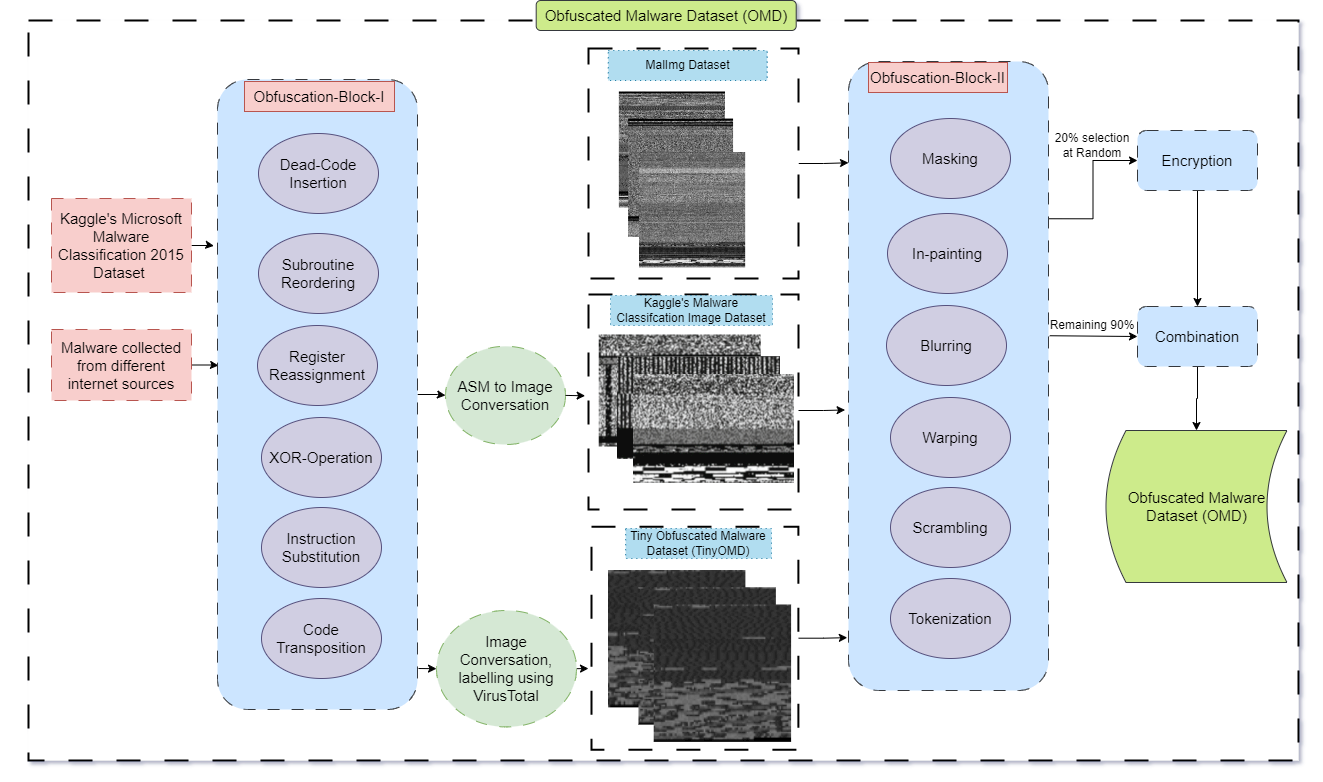
(a)

Figure 4: Dataset Generation Workflow

Table 9: Tiny Obfuscated Malware Dataset (TinyOMD)

Class	Number of Samples
Adware	16
Backdoor	8
Obfuscated	76
Other	177
Trojan	180
Virus	32
Total	489

Table 10: Obfuscated Malware Dataset (OMD))

S.No.	Family	Family Name	Number of samples
$1$	Dailer	Adialer.C	122
$2$	Adware	Various	16
$3$	Backdoor	Agent.FYI	116
$4$	Worm	Allaple.A	2949
$5$	Worm	Allaple.L	1591
$6$	Trojan	Alueron.gen!J	198
$7$	Worm:AutoIT	Autorun.K	106
$8$	Backdoor	Various	8
$9$	Trojan	C2lop.gen!G	200
$10$	Trojan	C2lop.p	146
$11$	Dailer	Diaplaform.B	177
$12$	TrojanDownloader	Dontovo.A	162
$13$	Rogue	Fakerean	381
$14$	Backdoor	Gatak	1013
$15$	Dailer	Instantaccess	431
$16$	Backdoor	Kelihos_ver1	398
$17$	Backdoor	Kelihos_ver3	2493
$18$	Adware	Lollipop	2476
$19$	PWS	Lolyda.AA1	213
$20$	PWS	Lolyda.AA2	184
$21$	PWS	Lolyda.AA3	123
$22$	PWS	Lolyda.AT	159
$23$	Trojan	Malex.gen!J	136
$24$	Obfuscated	Various	76
$25$	TrojanDownloader	Obfuscated.AD	1370
$26$	Any Obfuscated Malware	Obfuscator.ACY	1679
$27$	Various	Various	177
$28$	Worm	Ramnit	1541
$29$	Backdoor	Rbot!gen	158
$30$	Backdoor	Simda	42
$31$	Trojan	Skintrim.N	80
$32$	TrojanDownloader	Swizzor.gen!E	128
$33$	TrojanDownloader	Swizzor.gen!I	132
$34$	TrojanDownloader	Tracur	751
$35$	Trojan	Various	180
$36$	Worm	VB.AT	408
$37$	Virus	Various	32
$38$	Trojan	Vundo	475
$39$	TrojanDownloader	Wintrim.BX	97
$40$	Worm	Yuner.A	800
	Total		21924

3.2.3 Data augmentation

A lack of data causes deep learning models to overfit. To achieve effective generalisation and practical training, a large amount of data is therefore needed. Data augmentation is the process of increasing data samples by supplementing the underlying data Shorten and Khoshgoftaar (2019); Naveed et al. (2021). To enhance generality and make the suggested classification framework resistant to different types of malware data, we have expanded the training dataset in this study. Hence, it makes the suggested categorization system useful for categorising malware families. As illustrated in Table 11, the adopted augmentation technique incorporates a number of transformations, including reflections, scaling, rotation, and shear. To increase the generality of the models, all trainings are done after data augmentation.

Table 11: Augmentation parameters

S.No.	Augmentation type	Parameter
$1$	Rotate	[0, 360] degrees
$2$	Shear	[-0.1,0.1]
$3$	Reflection	X: [-1, 1],Y: [-1, 1]
$4$	Scale	[0.2, 1]
$5$	Horizontal Flip	-
$6$	Vertical Flip	-
$7$	Width Shift	[0, 0.2]
$8$	Height Shift	[0, 0.2]

3.2.4 Dataset Partitioning

In this study, the training and testing stages of the dataset partitioning strategy were 70-30. The literature often mentions dataset partitioning as 80-20, 75-25, or even 70-30. Hence, 70-30 was choosen to make the model robust. In this context, the dataset’s dimensions are important.

4 Performance Metrics

Prior to delving deeper into the performance measures, it was necessary to establish several fundamental units or classification categories, including TruePositive, TrueNegative, FalsePositive, and FalseNegative. To comprehend how each of these units is to be categorised, refer to Table .

1. TruePositive (TP): Both the actual and anticipated labels for the data sample are positive. If the model predicts class name of sample correctly out of 40 class names then it will be considered a true positive.

2. TrueNegative (TN): In multi-class classification, true negative is sum of all classes except for the class which is being under consideration.

3. FalsePositive (FP): False positive will represent sum of all classes except true positive in the corresponding columns.

4. FalseNegative (FN): Similarly, false negative will represent sum of all classes except true positive in the corresponding rows.

   4.1 Recall

   In multiclass classification, recall (also known as sensitivity or true positive rate) given in Eg. 12 is a metric that measures the proportion of true positive predictions for a given class out of all the actual positive instances in that class. It is defined as:

   $$Recall=\dfrac{TruePositive}{TruePositive+FalseNegative}$$ (1)

   where True positives are the number of correctly classified instances of a specific class, and False negatives are the number of instances that belong to that class but are incorrectly classified as belonging to a different class.

   In other words, recall in multiclass classification tells us how well the model is able to correctly identify all instances of a specific class, regardless of whether it misclassifies some instances from other classes as belonging to that class. A high recall value for a specific class indicates that the model is good at correctly identifying all instances of that class, while a low recall value indicates that the model is missing many instances of that class.

   4.2 Specificity

   Specificity is recall’s inverse, that is, it indicates how well a model is performing to correctly identify the negative labels. In simple words, specificity would be the ratio of TrueNegative to Total Negatives. Negative labels in our data would be the logs generated by benign applications. Specificity is calculated using formula given in Eq. 2.

   $$Specificity=\dfrac{TrueNegative}{TrueNegative+FalsePositive}$$ (2)

   4.3 Precision

   In multiclass classification, precision given in Eg. 12 is a metric that measures the proportion of true positive predictions for a given class out of all the positive predictions made by the model for that class. It is defined as:

   $$Precision=\dfrac{TruePositive}{TruePositive+FalsePositive}$$ (3)

   where True positives are the number of correctly classified instances of a specific class, and False positives are the number of instances that are incorrectly classified as belonging to that class, when in fact they belong to a different class.

   In other words, precision in multiclass classification tells us how well the model is able to correctly classify instances of a specific class, without misclassifying instances from other classes as belonging to that class. A high precision value for a specific class indicates that the model is good at correctly identifying instances of that class, while a low precision value indicates that the model is misclassifying many instances from other classes as belonging to that class.

   4.4 Accuracy

   Accuracy is how well the model is performing in correctly predicting the Positive and Negative Labels. It is the ratio correctly predicted to total samples. Eq. 12 is used to calculate the accuracy of any model.

   $$Accuracy=\dfrac{TruePositive+TrueNegative}{Totalnumberofsamples}$$ (4)

   4.5 F - Score

   F-score is also known as harmonic mean of precision and recall. This performance metric is highly suitable when it comes to imbalanced datasets. F-Score can be calculated using the model’s precision and recall given in 12.

   $$F-Score=2*\dfrac{precision*recall}{precision+recall}$$ (5)

Performance metrics are summarized in table 12.

Table 12: Summarized Performance Metrics

Name	Formula
Accuracy	$$\dfrac{TruePositive+TrueNegative}{Totalnumberofsamples}$$
Recall	$$\dfrac{TruePositive}{TruePositive+FalseNegative}$$
Precesion	$$\dfrac{TruePositive}{TruePositive+FalsePositive}$$
F1-Score	$$2*\dfrac{precision*recall}{precision+recall}$$

5 Traditional Machine Learning Classifiers

5.1 Decision Tree

Decision trees (DT) Charbuty and Abdulazeez (2021) are a non-parametric supervised leaning approach. DTs are very famous when it comes to classification and regression problems. Multiple decision rules are constructed which are inferred from various features of data. They are limited by the fact that they can be very non-robust. A small change in the training data can result in a large change in the tree and consequently the final predictions James et al. (2013). The problem of learning an optimal decision tree is known to be NP-complete under several aspects of optimality and even for simple concepts Laurent and Rivest (1976).

5.2 Bagging

Bagging also known as Bootstrap Aggregating Lee et al. (2020) is a technique in machine learning that involves combining multiple models trained on different subsets of the training data to improve predictive performance. The bagging technique works by creating multiple bootstrap samples of the training data and training a different model on each sample. By averaging the predictions of all the individual models, bagging can reduce overfitting and improve the stability and accuracy of the final prediction. Bagging can be applied to various machine learning algorithms, such as decision trees, neural networks, and random forests. The main benefits of bagging are improved accuracy, stability, and robustness, making it a popular technique in ensemble learning. Bagging is not always effective with data that has a high degree of correlation or has a very small number of informative features and may not always improve the performance of certain machine learning algorithms, such as k-nearest neighbors, that are inherently stable.

5.3 Gradient Boosting

Gradient boosting Zhang et al. (2019); Bentéjac et al. (2021) is a machine learning technique used in regression and classification tasks, among others. It gives a prediction model in the form of an ensemble of weak prediction models, which are typically decision trees. While boosting can increase the accuracy of a base learner, such as a decision tree or linear regression, it sacrifices intelligibility and interpretability.For example, following the path that a decision tree takes to make its decision is trivial and self-explained, but following the paths of hundreds or thousands of trees is much harder.

5.4 AdaBoost

AdaBoost, short for Adaptive Boosting Shahraki et al. (2020); Wang and Sun (2021), is a statistical classification meta-algorithm, Every learning algorithm tends to suit some problem types better than others, and typically has many different parameters and configurations to adjust before it achieves optimal performance on a dataset. AdaBoost (with decision trees as the weak learners) is often referred to as the best out-of-the-box classifier Kégl (2013). When used with decision tree learning, information gathered at each stage of the AdaBoost algorithm about the relative ’hardness’ of each training sample is fed into the tree growing algorithm such that later trees tend to focus on harder-to-classify examples. AdaBoost is particularly prone to overfitting on noisy datasets.

5.5 Support Vector Machine (SVM)

Support Vector Machine Kurani et al. (2023); Vos et al. (2022); Koklu et al. (2022) is a supervised learning method, which is used for problems such as classifying different classes (classification), predicting continuous value (Regression) and detection of any outliers. SVM is emplyed here because it is very effective in high dimensional spaces, and our dataset has deep feature space. Another reason for using SVM is that it is very memory efficient as it uses a subset of training samples in decision function. When devising the architecture of SVM approach there were 3 primary parameters of concern, Kernel function, gamma, and C. Gamma dictates how much influence can a single sample in training space has. A lower value of C indicates the decision surface of the classifier to be smooth, which means that there can some percentage of mis-classification allowed. However, if C is set to a higher value, then SVM aims to classify all the training samples correctly, and percentage of error or mis-classification is reduced. Different values of these that were evaluated are given in table 13.

Table 13: SVM model variations

Kernel	C-Parameter	Gamma
Linear	1	0.1
	5	0.1
	10	0.1
Radial Basis Function	1	0.1
	5	0.1
	10	0.1

5.6 Random Forest (RF)

When multiple decision trees are combined, and are used as an ensemble strategy to improve the accuracy, this architecture is known as Random Forest Balyan et al. (2022); Wang et al. (2023). Key parameter for Random forest is the $n\_estimators$ which indicates the number of trees to be used in forest. Another vital parameter is the $max\_depth$ of the trees in forest which limits the number of splits/divisions that can be performed per tree. Table 14 gives parameters applied during training using RF.

Table 14: RF model variations

n-estimators	Depth of trees
100	10
	20
	30
	40
200	10
	20

5.7 XGBoost

XGBoost Velarde et al. (2023) (eXtreme Gradient Boosting) is an open-source software library which provides a regularizing gradient boosting. Salient features of XGBoost which make it different from other gradient boosting algorithms are clever penalization of trees, proportional shrinking of leaf nodes, Newton Boosting, extra randomization parameter, implementation on single, distributed systems and out-of-core computation and automatic feature selection. It is known for its superior performance in various machine learning tasksZhang et al. (2018); Chen et al. (2019); Jiang et al. (2019), including malware analysis, for the following reasons: it effectively handles complex relationships and captures intricate patterns within the data, which is essential for accurately detecting and classifying obfuscated malware. XGBoost employs regularization techniques to prevent overfitting and build robust models that generalize well to unseen malware samples. Built on the gradient boosting framework, it learns from previous models’ mistakes and leverages the strengths of multiple decision trees to achieve high accuracy. XGBoost includes strategies to handle class imbalance, ensuring effective learning from imbalanced data. Additionally, it offers computational efficiency, scalability, and the ability to handle large-scale analysis efficiently, crucial for processing extensive malware datasets.

5.8 Voting

Voting ensemble Hussain et al. (2023); Zhang et al. (2023); Sevim et al. (2023); Mohammadifar et al. (2023) is a machine learning technique that combines multiple models trained on the same dataset to improve the overall predictive power of the system. In voting ensemble, each model is given an equal vote, and the final prediction is based on the majority vote of all the models. By combining multiple models trained on the same dataset, voting ensemble can often achieve higher accuracy than any individual model but this leads to complexity and makes it computationally expensive than individual models, as it requires training and combining multiple models. It can reduce the risk of overfitting, as it combines multiple models with different biases and strengths, which helps to reduce the variance in the final predictions and is often more robust than individual models, as it can handle missing or noisy data more effectively by combining the predictions of multiple models. But it may not be effective if the individual models are too similar, as it can lead to over-reliance on certain features or biases and most importantly requires training multiple models, which can be time-consuming and resource-intensive.

6 Experimental Environment

Hardware and software resources employed during experiments are given in table 15 and 16, respectively.

Table 15: Hardware Resources

Name of hardware	Specification
Intel(R) Core(TM) i7-8700	CPU @ 3.20GHz
RAM	32GB

Table 16: Software Resources

Name of software	Source	Description
Python3.9.15	www.python.org	Platform independent programming language (open source)
TensorFlow2.10.0	www.tensorflow.org/	End-to-end learning framework for deploying machine learning models (open source)
Pytorch1.13.1	www.pytorch.org	Large-scale deep machine learning library (open source)
Scikit-learn	www.scikit-learn.org/stable/	Simple open-source efficient predictive data analysis tool
Microsoft Windows 11	www.microsoft.com/en-us/windows/?r=1	The most recent major version of Microsoft’s Windows NT operating system

7 Results and Discussion

Table 17: Results

Classifier(s)	Precision	Recall	F-1 Score	Accuracy
Decision Tree	74	76	72	75
Logistic Regression	82	72	69	76
Random Forest	91	77	79	82
XGBoost	88	80	82	83
SVM	83	71	76	73
AdaBoostClassifier	88	76	76	80
Ensemble (Voting:SVM+LR)	79	77	77	77

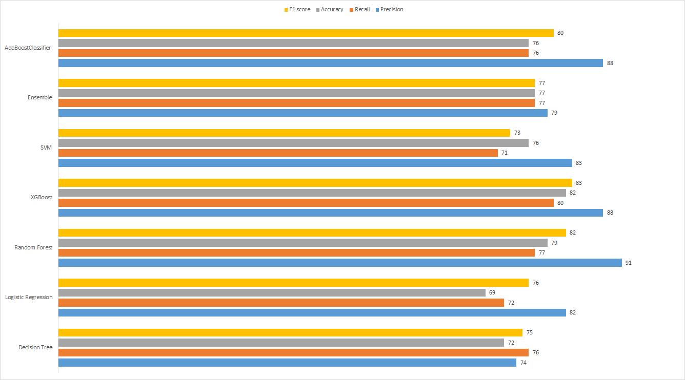
(a)

Figure 5: Comparison between Decision Trees, AdaBoost, SVM, RF, Logistic Regression, XGBoost, and Ensemble of SVM and LR using Recall, Accuracy, Precision and F-Score, XGBoost and RF are best performing ones

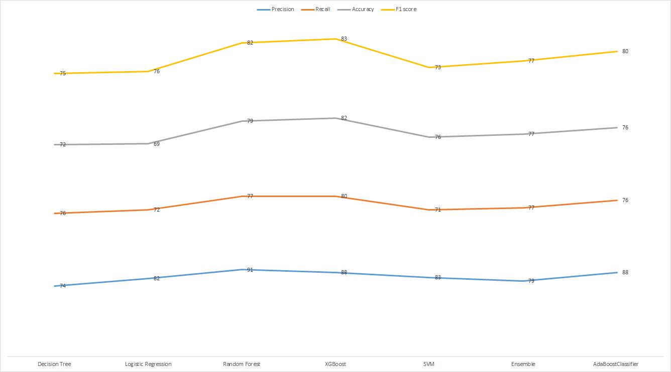
(a)

Figure 6: XGBoost and RF perform best with RF edging it on precision while in other three metrics XGBoost performs better

Results demonstrate that XGBoost outperforms all other methods achieving an accuracy, precision, recall, F1-Score of 82%, 88%, 80% and 83% respectively as shown in fig. 5. RF has the highest precision shown in fig. 6 at 88% but in other three metrics XGBoost performs better and overall gives a better result.

8 Conclusion

With the rise in computer usage, cybersecurity has emerged as a crucial concern in the digital era. Cybercriminals have expanded their activities beyond traditional hacking and virus distribution. Daily malware attacks inflict significant financial losses by targeting computer users, businesses, and government agencies. Despite the availability of diverse security tools, malware can evade detection by making clever adjustments, causing significant challenges for security experts. To address this issue, the Obfuscated Malware Dataset (OMD) is introduced, consisting of 21,924 samples from 40 distinct malware families. The dataset incorporates various obfuscation techniques, simulating the tactics employed by malware authors to create new strains. Robust models utilizing traditional machine learning algorithms, such as SVM, RF, XGBOOST, and others, are trained to effectively identify these evasive malware instances that are difficult to detect through conventional means.

References

- Gao et al. (2019) Jun Gao, Li Li, Pingfan Kong, Tegawendé F Bissyandé, and Jacques Klein. Should you consider adware as malware in your study? In 2019 IEEE 26th International Conference on Software Analysis, Evolution and Reengineering (SANER), pages 604–608. IEEE, 2019.
- Kumar and Subbiah (2022) Rajesh Kumar and Geetha Subbiah. Zero-day malware detection and effective malware analysis using shapley ensemble boosting and bagging approach. Sensors, 22(7):2798, 2022.
- Barros et al. (2022) Pedro H Barros, Eduarda TC Chagas, Leonardo B Oliveira, Fabiane Queiroz, and Heitor S Ramos. Malware-smell: A zero-shot learning strategy for detecting zero-day vulnerabilities. Computers & Security, 120:102785, 2022.
- Botacin et al. (2022) Marcus Botacin, Marco Zanata Alves, Daniela Oliveira, and André Grégio. Heaven: A hardware-enhanced antivirus engine to accelerate real-time, signature-based malware detection. Expert Systems with Applications, 201:117083, 2022.
- Selamat and Ali (2022) Nur Syuhada Selamat and Fakariah Hani Mohd Ali. Polymorphic malware detection based on supervised machine learning. Journal of Positive School Psychology, 6(3):8538–8547, 2022.
- Brewer (2016) Ross Brewer. Ransomware attacks: detection, prevention and cure. Network Security, 2016(9):5–9, 2016.
- Tahir (2018) Rabia Tahir. A study on malware and malware detection techniques. International Journal of Education and Management Engineering, 8(2):20, 2018.
- Menn (2010) Joseph Menn. Fatal system error: the hunt for the new crime lords who are bringing down the internet. PublicAffairs, 2010.
- Geer and Conway (2009) Daniel E Geer and Daniel G Conway. the 0wned price index. IEEE Security & Privacy, 7(1):86–87, 2009.
- Salloum et al. (2022) Said Salloum, Tarek Gaber, Sunil Vadera, and Khaled Sharan. A systematic literature review on phishing email detection using natural language processing techniques. IEEE Access, 2022.
- Wang et al. (2021) Haojun Wang, Haixia Long, Ailan Wang, Tianyue Liu, and Haiyan Fu. Deep learning and regularization algorithms for malicious code classification. IEEE Access, 9:91512–91523, 2021.
- Grammatikakis et al. (2021) Konstantinos P Grammatikakis, Ioannis Koufos, Nicholas Kolokotronis, Costas Vassilakis, and Stavros Shiaeles. Understanding and mitigating banking trojans: From zeus to emotet. In 2021 IEEE International Conference on Cyber Security and Resilience (CSR), pages 121–128. IEEE, 2021.
- Kazi et al. (2022) Mohamed Ali Kazi, Steve Woodhead, and Diane Gan. Comparing the performance of supervised machine learning algorithms when used with a manual feature selection process to detect zeus malware. International Journal of Grid and Utility Computing, 13(5):495–504, 2022.
- Rose et al. (2022) Joseph R Rose, Matthew Swann, Konstantinos P Grammatikakis, Ioannis Koufos, Gueltoum Bendiab, Stavros Shiaeles, and Nicholas Kolokotronis. Ideres: Intrusion detection and response system using machine learning and attack graphs. Journal of Systems Architecture, 131:102722, 2022.
- Nataraj et al. (2011) Lakshmanan Nataraj, Sreejith Karthikeyan, Gregoire Jacob, and Bangalore S Manjunath. Malware images: visualization and automatic classification. In Proceedings of the 8th international symposium on visualization for cyber security, pages 1–7, 2011.
- Gibert et al. (2019) Daniel Gibert, Carles Mateu, Jordi Planes, and Ramon Vicens. Using convolutional neural networks for classification of malware represented as images. Journal of Computer Virology and Hacking Techniques, 15:15–28, 2019.
- Ronen et al. (2018) Royi Ronen, Marian Radu, Corina Feuerstein, Elad Yom-Tov, and Mansour Ahmadi. Microsoft malware classification challenge. arXiv preprint arXiv:1802.10135, 2018.
- Kancherla and Mukkamala (2013) Kesav Kancherla and Srinivas Mukkamala. Image visualization based malware detection. In 2013 IEEE Symposium on Computational Intelligence in Cyber Security (CICS), pages 40–44. IEEE, 2013.
- Ahmadi et al. (2016) Mansour Ahmadi, Dmitry Ulyanov, Stanislav Semenov, Mikhail Trofimov, and Giorgio Giacinto. Novel feature extraction, selection and fusion for effective malware family classification. In Proceedings of the sixth ACM conference on data and application security and privacy, pages 183–194, 2016.
- Rezende et al. (2017) Edmar Rezende, Guilherme Ruppert, Tiago Carvalho, Fabio Ramos, and Paulo De Geus. Malicious software classification using transfer learning of resnet-50 deep neural network. In 2017 16th IEEE International Conference on Machine Learning and Applications (ICMLA), pages 1011–1014. IEEE, 2017.
- Qiao et al. (2016) Yanchen Qiao, Xiaochun Yun, and Yongzheng Zhang. How to automatically identify the homology of different malware. In 2016 IEEE Trustcom/BigDataSE/ISPA, pages 929–936. IEEE, 2016.
- Karbab et al. (2018) ElMouatez Billah Karbab, Mourad Debbabi, Abdelouahid Derhab, and Djedjiga Mouheb. Maldozer: Automatic framework for android malware detection using deep learning. Digital Investigation, 24:S48–S59, 2018.
- Arp et al. (2014) Daniel Arp, Michael Spreitzenbarth, Malte Hubner, Hugo Gascon, Konrad Rieck, and CERT Siemens. Drebin: Effective and explainable detection of android malware in your pocket. In Ndss, volume 14, pages 23–26, 2014.
- Anderson and Roth (2018) Hyrum S Anderson and Phil Roth. Ember: an open dataset for training static pe malware machine learning models. arXiv preprint arXiv:1804.04637, 2018.
- Sebastián et al. (2016) Marcos Sebastián, Richard Rivera, Platon Kotzias, and Juan Caballero. Avclass: A tool for massive malware labeling. In Research in Attacks, Intrusions, and Defenses: 19th International Symposium, RAID 2016, Paris, France, September 19-21, 2016, Proceedings 19, pages 230–253. Springer, 2016.
- Plohmann et al. (2017) Daniel Plohmann, Martin Clauss, Steffen Enders, and Elmar Padilla. Malpedia: a collaborative effort to inventorize the malware landscape. Proceedings of the Botconf, 2017.
- Kotzias et al. (2015) Platon Kotzias, Srdjan Matic, Richard Rivera, and Juan Caballero. Certified pup: abuse in authenticode code signing. In Proceedings of the 22nd ACM SIGSAC Conference on Computer and Communications Security, pages 465–478, 2015.
- Huang and Stokes (2016) Wenyi Huang and Jack W Stokes. Mtnet: a multi-task neural network for dynamic malware classification. In Detection of Intrusions and Malware, and Vulnerability Assessment: 13th International Conference, DIMVA 2016, San Sebastián, Spain, July 7-8, 2016, Proceedings 13, pages 399–418. Springer, 2016.
- Shorten and Khoshgoftaar (2019) Connor Shorten and Taghi M Khoshgoftaar. A survey on image data augmentation for deep learning. Journal of big data, 6(1):1–48, 2019.
- Naveed et al. (2021) Humza Naveed, Saeed Anwar, Munawar Hayat, Kashif Javed, and Ajmal Mian. Survey: Image mixing and deleting for data augmentation. arXiv preprint arXiv:2106.07085, 2021.
- Charbuty and Abdulazeez (2021) Bahzad Charbuty and Adnan Abdulazeez. Classification based on decision tree algorithm for machine learning. Journal of Applied Science and Technology Trends, 2(01):20–28, 2021.
- James et al. (2013) Gareth James, Daniela Witten, Trevor Hastie, and Robert Tibshirani. An introduction to statistical learning, volume 112. Springer, 2013.
- Laurent and Rivest (1976) Hyafil Laurent and Ronald L Rivest. Constructing optimal binary decision trees is np-complete. Information processing letters, 5(1):15–17, 1976.
- Lee et al. (2020) Tae-Hwy Lee, Aman Ullah, and Ran Wang. Bootstrap aggregating and random forest. Macroeconomic forecasting in the era of big data: Theory and practice, pages 389–429, 2020.
- Zhang et al. (2019) Zhongheng Zhang, Yiming Zhao, Aran Canes, Dan Steinberg, Olga Lyashevska, et al. Predictive analytics with gradient boosting in clinical medicine. Annals of translational medicine, 7(7), 2019.
- Bentéjac et al. (2021) Candice Bentéjac, Anna Csörgő, and Gonzalo Martínez-Muñoz. A comparative analysis of gradient boosting algorithms. Artificial Intelligence Review, 54:1937–1967, 2021.
- Shahraki et al. (2020) Amin Shahraki, Mahmoud Abbasi, and Øystein Haugen. Boosting algorithms for network intrusion detection: A comparative evaluation of real adaboost, gentle adaboost and modest adaboost. Engineering Applications of Artificial Intelligence, 94:103770, 2020.
- Wang and Sun (2021) Wenyang Wang and Dongchu Sun. The improved adaboost algorithms for imbalanced data classification. Information Sciences, 563:358–374, 2021.
- Kégl (2013) Balázs Kégl. The return of adaboost. mh: multi-class hamming trees. arXiv preprint arXiv:1312.6086, 2013.
- Kurani et al. (2023) Akshit Kurani, Pavan Doshi, Aarya Vakharia, and Manan Shah. A comprehensive comparative study of artificial neural network (ann) and support vector machines (svm) on stock forecasting. Annals of Data Science, 10(1):183–208, 2023.
- Vos et al. (2022) Kilian Vos, Zhongxiao Peng, Christopher Jenkins, Md Rifat Shahriar, Pietro Borghesani, and Wenyi Wang. Vibration-based anomaly detection using lstm/svm approaches. Mechanical Systems and Signal Processing, 169:108752, 2022.
- Koklu et al. (2022) Murat Koklu, M Fahri Unlersen, Ilker Ali Ozkan, M Fatih Aslan, and Kadir Sabanci. A cnn-svm study based on selected deep features for grapevine leaves classification. Measurement, 188:110425, 2022.
- Balyan et al. (2022) Amit Kumar Balyan, Sachin Ahuja, Umesh Kumar Lilhore, Sanjeev Kumar Sharma, Poongodi Manoharan, Abeer D Algarni, Hela Elmannai, and Kaamran Raahemifar. A hybrid intrusion detection model using ega-pso and improved random forest method. Sensors, 22(16):5986, 2022.
- Wang et al. (2023) Jing Wang, Congjun Rao, Mark Goh, and Xinping Xiao. Risk assessment of coronary heart disease based on cloud-random forest. Artificial Intelligence Review, 56(1):203–232, 2023.
- Velarde et al. (2023) Gissel Velarde, Anindya Sudhir, Sanjay Deshmane, Anuj Deshmunkh, Khushboo Sharma, and Vaibhav Joshi. Evaluating xgboost for balanced and imbalanced data: Application to fraud detection. arXiv preprint arXiv:2303.15218, 2023.
- Zhang et al. (2018) Dahai Zhang, Liyang Qian, Baijin Mao, Can Huang, Bin Huang, and Yulin Si. A data-driven design for fault detection of wind turbines using random forests and xgboost. Ieee Access, 6:21020–21031, 2018.
- Chen et al. (2019) Minghua Chen, Qunying Liu, Shuheng Chen, Yicen Liu, Chang-Hua Zhang, and Ruihua Liu. Xgboost-based algorithm interpretation and application on post-fault transient stability status prediction of power system. IEEE Access, 7:13149–13158, 2019.
- Jiang et al. (2019) Yu Jiang, Guoxiang Tong, Henan Yin, and Naixue Xiong. A pedestrian detection method based on genetic algorithm for optimize xgboost training parameters. IEEE Access, 7:118310–118321, 2019.
- Hussain et al. (2023) Muhammad Hussain, Hatim A AboAlSamh, Ihsan Ullah, et al. Emotion recognition system based on two-level ensemble of deep-convolutional neural network models. IEEE Access, 11:16875–16895, 2023.
- Zhang et al. (2023) Tie Zhang, Jingfu Zheng, and Yanbiao Zou. Weighted voting ensemble method for predicting workpiece imaging dimensional deviation based on monocular vision systems. Optics & Laser Technology, 159:109012, 2023.
- Sevim et al. (2023) Semih Sevim, Sevinç İlhan Omurca, and Ekin Ekinci. Improving accuracy of document image classification through soft voting ensemble. In Smart Applications with Advanced Machine Learning and Human-Centred Problem Design, pages 161–173. Springer, 2023.
- Mohammadifar et al. (2023) Aliakbar Mohammadifar, Hamid Gholami, and Shahram Golzari. Stacking-and voting-based ensemble deep learning models (sedl and vedl) and active learning (al) for mapping land subsidence. Environmental Science and Pollution Research, 30(10):26580–26595, 2023.