A Computational Framework for Solving
Wasserstein Lagrangian Flows

Abstract

The dynamical formulation of the optimal transport can be extended through various choices of the underlying geometry (kinetic energy), and the regularization of density paths (potential energy). These combinations yield different variational problems (Lagrangians), encompassing many variations of the optimal transport problem such as the Schrödinger bridge, unbalanced optimal transport, and optimal transport with physical constraints, among others. In general, the optimal density path is unknown, and solving these variational problems can be computationally challenging. Leveraging the dual formulation of the Lagrangians, we propose a novel deep learning based framework approaching all of these problems from a unified perspective. Our method does not require simulating or backpropagating through the trajectories of the learned dynamics, and does not need access to optimal couplings. We showcase the versatility of the proposed framework by outperforming previous approaches for the single-cell trajectory inference, where incorporating prior knowledge into the dynamics is crucial for correct predictions.

1 Introduction

The problem of trajectory inference, or recovering the population dynamics of a system from samples of its temporal marginal distributions, is a problem arising throughout the natural sciences (Hashimoto et al., 2016; Lavenant et al., 2021). A particularly important application is analysis of single-cell RNA-sequencing data (Schiebinger et al., 2019; Schiebinger, 2021; Saelens et al., 2019), which provides a heterogeneous snapshot of a cell population at a high resolution, allowing high-throughput observation over tens of thousands of genes (Macosko et al., 2015). However, since the measurement process ultimately leads to cell death, we can only observe temporal changes of the marginal or population distributions of cells as they undergo treatment, differentiation, or developmental processes of interest. To understand these processes and make future predictions, we are interested in both (i) interpolating the evolution of marginal cell distributions between observed timepoints and (ii) modeling the full trajectories at the individual cell level.

However, when inferring trajectories over cell distributions, there exist multiple cell dynamics that yield the same population marginals. This presents an ill-posed problem, which highlights the need for trajectory inference methods to be able to flexibly incorporate different types of prior information on the cell dynamics. Commonly, such prior information is specified via posing a variational problem on the space of marginal distributions, where previous work on measure-valued splines (Chen et al., 2018; Benamou et al., 2019; Chewi et al., 2021; Clancy & Suarez, 2022; Chen et al., 2023) are examples which seek minimize the acceleration of particles.

We propose a general framework for using deep neural networks to infer dynamics and solve marginal interpolation problems, using Lagrangian action functionals on manifolds of probability measures that can flexibly incorporate various types of prior information. We consider Lagrangians of the form ${\mathcal{L}}[\rho_{t},\dot{\rho}_{t},t]={\mathcal{K}}[\rho_{t},\dot{\rho}_{t},t]-{\mathcal{U}}[\rho_{t},t]$, referring to the first term as a kinetic energy and the second as a potential energy. Our methods can be used to solve a diverse family of problems defined by the choice of these energies and constraints on the evolution of $\rho_{t}$. More explicitly, we specify

• A kinetic energy which, in the primary examples considered in this paper, corresponds to a geometry on the space of probability measures. We primarily consider the Riemannian structures corresponding to the Wasserstein-2 and Wasserstein Fisher-Rao metrics.

• A potential energy, which may include functionals of the density such as the Shannon entropy, or spatial potentials which encode physical prior knowledge.

• A collection of marginal constraints which are inspired by the availability of data in the problem of interest. For optimal transport (ot), Schrödinger Bridge (sb), or generative modeling tasks, we are often interested in interpolating between two endpoint marginals given by a data distribution and/or a tractable prior distribution. For applications in trajectory inference, we may incorporate multiple constraints to match the observed temporal marginals, given via data samples. Notably, in the limit of data sampled infinitely densely in time, we recover the Action Matching (am) framework of Neklyudov et al. (2023).

Within our Wasserstein Lagrangian Flows framework, we propose tractable dual objectives to solve (i) standard Wasserstein-2 ot (Ex. 4.1, Benamou & Brenier (2000); Villani (2009)), (ii) entropy regularized ot or Schrödinger Bridge (Ex. 4.4, Léonard (2013); Chen et al. (2021b), (iii) physically constrained ot (Ex. 4.3, Villani (2009); Tong et al. (2020); Koshizuka & Sato (2022)), and (iv) unbalanced ot (Ex. 4.2, Liero et al. (2016); Kondratyev et al. (2016); Chizat et al. (2018a)) problems (Sec. 4). Our framework also allows for combining energy terms to incorporate various features of the above problems as inductive biases for trajectory inference. In Sec. 5, we showcase the ability of our methods to accurately solve Lagrangian flow optimization problems, and highlight how considering different Lagrangians can improve results for single-cell RNA-sequencing applications. We discuss benefits of our approach compared to related work in Sec. 6.

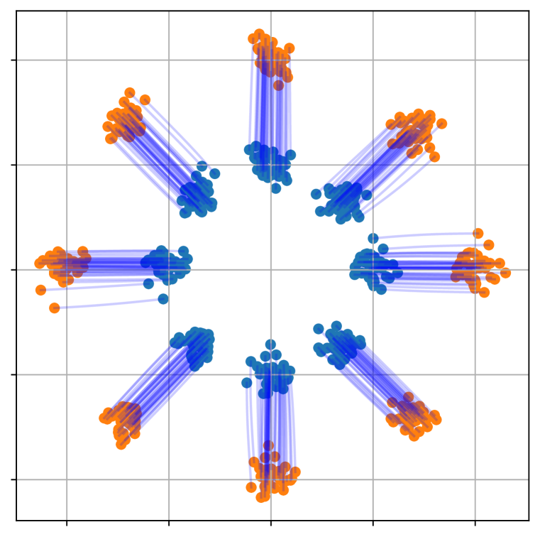
(a) Unregularized ot

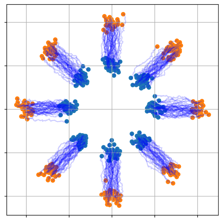
(b) sb/Entropic ot

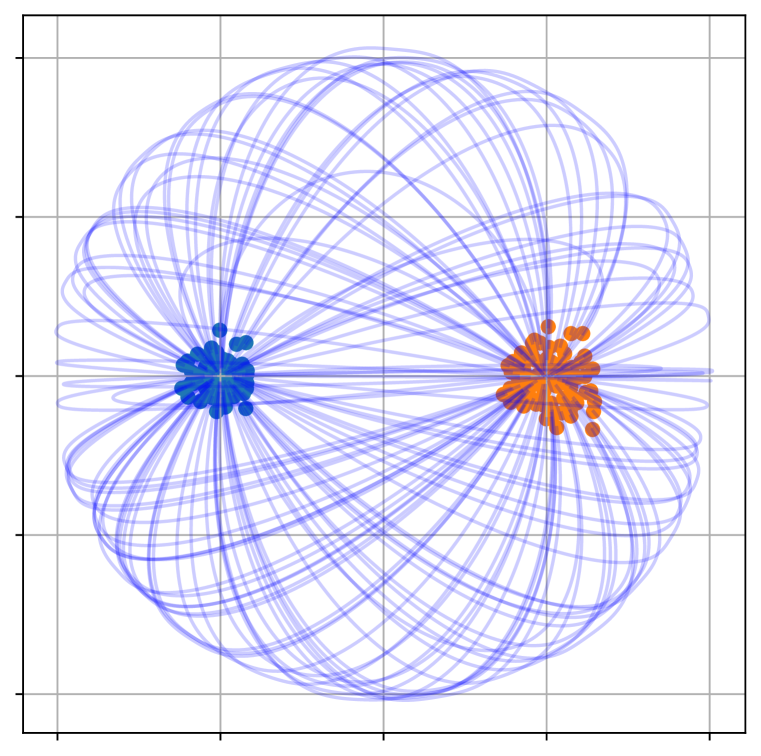
(c) Physical ot

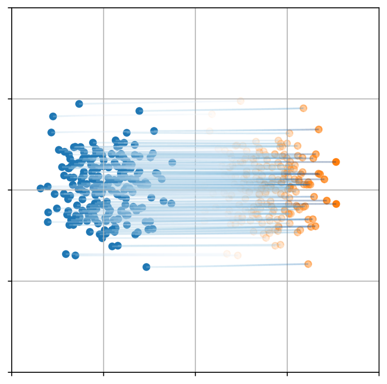
(d) Unbalanced ot

Figure 1: Toy examples for different Wasserstein Lagrangian Flows considered in this paper.

2 Background

2.1 Lagrangian and Hamiltonian Mechanics

We begin by reviewing action-minimizing curves in the ground space, which forms the basis the Lagrangian formulation of classical mechanics (Arnol’d, 2013). For curves $\gamma(t):[0,1]\rightarrow{\mathcal{X}}$ with velocity $\dot{\gamma}_{t}\in{\mathcal{T}}_{\gamma(t)}{\mathcal{X}}$, we consider evaluating a Lagrangian function $L(\gamma_{t},\dot{\gamma}_{t},t)$ along the curve to define the action as the time integral ${\mathcal{A}}(\gamma)=\int_{0}^{1}L(\gamma_{t},\dot{\gamma}_{t},t)dt$. Given two endpoints $x_{0},x_{1}\in{\mathcal{X}}$, we consider minimizing the action along all curves with the appropriate endpoints $\gamma\in\Pi(x_{0},x_{1})$,

$$c(x_{0},x_{1})=\inf\limits_{\gamma\in\Pi(x_{0},x_{1})}{\mathcal{A}}(\gamma)=\inf\limits_{\gamma_{t}}\int_{0}^{1}L(\gamma_{t},\dot{\gamma}_{t},t)dt\quad\text{s.t.}\,\,\gamma_{0}=x_{0},\,\,\gamma_{1}=x_{1}$$ (1)

We refer to the optimizing curves $\gamma^{*}(x_{0},x_{1})$ as Lagrangian flows in the ground-space, which satisfy the Euler-Lagrange equation $\frac{d}{dt}\frac{\partial}{\partial\dot{\gamma}_{t}}L(\gamma_{t},\dot{\gamma}_{t},t)=\frac{d}{d\gamma_{t}}L(\gamma_{t},\dot{\gamma}_{t},t)$ as a stationarity condition.

We will assume that $L(\gamma_{t},\dot{\gamma}_{t},t)$ is strictly convex in the velocity $\dot{\gamma}_{t}$, in which case we can obtain an equivalent, Hamiltonian perspective via convex duality. Considering momentum variables $p_{t}$, we define the Hamiltonian $H(\gamma_{t},p_{t},t)$ as the Legendre transform of $L$ with respect to $\dot{\gamma}_{t}$,

$$H(\gamma_{t},p_{t},t)=\sup\limits_{\dot{\gamma}_{t}}~{}\langle\dot{\gamma}_{t},p_{t}\rangle-L(\gamma_{t},\dot{\gamma}_{t},t)$$ (2)

The Euler-Lagrange equations can be written as Hamilton’s equations in the phase space

$$\dot{\gamma}_{t}=\frac{\partial}{\partial p_{t}}H(\gamma_{t},p_{t},t)\qquad\qquad\dot{p}_{t}=-\frac{\partial}{\partial\gamma_{t}}H(\gamma_{t},p_{t},t).$$ (3)

The remainder of this paper is devoted to lifting these concepts to the space of probability densities and deriving tractable optimization techniques to solve for the resulting Lagrangian flows.

2.2 Wasserstein-2 Geometry

For two given densities with finite second moments $\mu_{0},\mu_{1}\in{\mathcal{P}}_{2}({\mathcal{X}})$, the Wasserstein-2 ot problem is defined, in the Kantorovich formulation, as a cost-minimization problem over joint distributions or ‘couplings’ $\pi\in\Pi(\mu_{0},\mu_{1})=\{\pi(x_{0},x_{1})\,|\,\int\pi(x_{0},x_{1})dx_{1}=\mu_{0},\;\int\pi(x_{0},x_{1})dx_{0}=\mu_{1}\}$, i.e.

$$W_{2}(\mu_{0},\mu_{1})^{2}\coloneqq\inf\limits_{\pi\in\Pi(\mu_{0},\mu_{1})}\int\|x_{0}-x_{1}\|^{2}\pi(x_{0},x_{1})dx_{0}dx_{1}\,.$$ (4)

The dynamical formulation of Benamou & Brenier (2000) gives an alternative perspective on the $W_{2}$ ot problem as an optimization over a vector field $v_{t}$ that transports samples according to an ode $\dot{x}_{t}=v_{t}$. The evolution of the samples’ density $\rho_{t}$, under transport by $v_{t}$, is governed by the continuity equation $\dot{\rho}_{t}=-\nabla\cdot\mathopen{}\mathclose{{}\left(\rho_{t}v_{t}}\right)$ (Figalli & Glaudo (2021) Lemma 4.1.1), and we have

$$W_{2}(\mu_{0},\mu_{1})^{2}= ~{}\inf\limits_{\rho_{t}}\inf\limits_{v_{t}}\int_{0}^{1}\int\frac{1}{2}{\|v_{t}\|^{2}}~{}\rho_{t}~{}dx_{t}dt\quad\text{s.t.}\,\,\dot{\rho}_{t}=-\nabla\cdot\mathopen{}\mathclose{{}\left(\rho_{t}v_{t}}\right),\,\,~{}\rho_{0}=\mu_{0},\,\,\rho_{1}=\mu_{1},$$ (5)

where $\nabla\cdot\mathopen{}\mathclose{{}\left(}\right)$ is the divergence operator. The $W_{2}$ transport cost can be viewed as providing a Riemannian manifold structure on the space of densities ${\mathcal{P}}_{2}({\mathcal{X}})$ (Otto (2001); Ambrosio et al. (2008), see also Figalli & Glaudo (2021) Ch. 4). Introducing Lagrange multipliers $s_{t}$ to enforce the constraints in Eq. 5, we obtain the condition that $v_{t}=\nabla s_{t}$ (see Sec. B.1), which is suggestive of the result from Ambrosio et al. (2008) characterizing the tangent space $T^{W_{2}}_{\rho}{\mathcal{P}}_{2}=\{\dot{\rho}~{}|\int\dot{\rho}~{}dx_{t}=0\}$ via the continuity equation,

$$T^{W_{2}}_{\rho}{\mathcal{P}}_{2}({\mathcal{X}})=\{\dot{\rho}~{}|~{}\dot{\rho}=-\nabla\cdot\mathopen{}\mathclose{{}\left(\rho\nabla s}\right)\}.$$ (6)

We also write the cotangent space as $T^{*W_{2}}_{\rho}{\mathcal{P}}_{2}({\mathcal{X}})=\{[s]~{}|~{}s\in{\mathcal{C}}^{\infty}(\mathcal{X})\}$, where ${\mathcal{C}}^{\infty}(\mathcal{X})$ denotes smooth functions and $[s]$ is an equivalence class up to addition by a constant.

For two curves $\mu_{t},\rho_{t}:[-\epsilon,\epsilon]\mapsto{\mathcal{P}}_{2}({\mathcal{X}})$ passing through $\rho\coloneqq\rho_{0}=\mu_{0}$, the Otto metric is defined

$$\langle\dot{\mu}_{t},\dot{\rho}_{t}\rangle^{W_{2}}_{T_{\rho}}=\langle s_{\dot{\mu}_{t}},s_{\dot{\rho}_{t}}\rangle_{T^{*}_{\rho}}^{W_{2}}=\int\langle\nabla s_{\dot{\mu}_{t}},\nabla s_{\dot{\rho}_{t}}\rangle\rho~{}dx.$$ (7)

2.3 Wasserstein Fisher-Rao Geometry

Building from the dynamical formulation in Eq. 5, Chizat et al. (2018a; b); Kondratyev et al. (2016); Liero et al. (2016; 2018) consider additional terms allowing for birth and death of particles, or teleportation of probability mass. In particular, consider extending the continuity equation to include a ‘growth term’ $g_{t}:{\mathcal{X}}\rightarrow\mathbb{R}$ whose norm is regularized in the cost,

$$WFR_{\lambda}(\mu_{0},\mu_{1})^{2}=\inf\limits_{\rho_{t}}\inf\limits_{v_{t},g_{t}}\int_{0}^{1}\int\mathopen{}\mathclose{{}\left(\frac{1}{2}\|v_{t}\|^{2}+\frac{\lambda}{2}g_{t}^{2}}\right)~{}\rho_{t}~{}dx_{t}dt,$$ (8)

subject to $\dot{\rho}_{t}=-\nabla\cdot\mathopen{}\mathclose{{}\left(\rho_{t}v_{t}}\right)+\lambda\rho_{t}g_{t},\rho_{0}=\mu_{0},\rho_{1}=\mu_{1}$. We call this the Wasserstein Fisher-Rao (wfr) distance, since considering only the growth terms recovers the non-parametric Fisher-Rao metric (Chizat et al., 2018a; Bauer et al., 2016). We also refer to Eq. 8 as the unbalanced ot problem on the space of unnormalized densities ${\mathcal{M}}({\mathcal{X}})$, since the growth terms need not preserve normalization $\int\dot{\rho}_{t}dx_{t}=\int\lambda g_{t}\rho_{t}dx_{t}\neq 0$ without further modifications (see e.g. Lu et al. (2019)).

Kondratyev et al. (2016) define a Riemannian structure on ${\mathcal{M}}({\mathcal{X}})$ via the wfr distance. Introducing Lagrange multipliers $s_{t}$ and eliminating $v_{t},g_{t}$ in Eq. 8 yields the optimality conditions $v_{t}=\nabla s_{t}$ and $g_{t}=s_{t}$. In analogy with Sec. 2.2, this suggests characterizing the tangent space via the tuple $(s_{t},\nabla s_{t})$ and defining the metric as

$$T^{WFR_{\lambda}}_{\rho}{\mathcal{M}}({\mathcal{X}}) =\{\dot{\rho}~{}|~{}\dot{\rho}=-\nabla\cdot\mathopen{}\mathclose{{}\left(\rho\nabla s}\right)+\lambda\rho s\}\qquad$$ (9)

$$\langle\dot{\mu}_{t},\dot{\rho}_{t}\rangle^{WFR_{\lambda}}_{T_{\rho}} =\langle s_{\dot{\mu}_{t}},s_{\dot{\rho}_{t}}\rangle^{WFR_{\lambda}}_{T^{*}_{\rho}}=\int\big{(}\vphantom{\frac{1}{2}}\langle\nabla s_{\dot{\mu}_{t}},\nabla s_{\dot{\rho}_{t}}\rangle+\lambda~{}s_{\dot{\mu}_{t}}s_{\dot{\rho}_{t}}\big{)}\rho~{}dx.$$ (10)

2.4 Action Matching

Finally, Action Matching (am) (Neklyudov et al., 2023) considers only the inner optimizations in Eq. 5 or Eq. 8 as a function of $v_{t}$ or $(v_{t},g_{t})$, assuming a distributional paths $\mu_{t}$ is given via samples. In the $W_{2}$ case, to solve for the velocity $v_{t}=\nabla s_{\dot{\mu}_{t}}$ which corresponds to $\mu_{t}$ via the continuity equation or Eq. 6, Neklyudov et al. (2023) optimize the objective

$${\mathcal{A}}[\mu_{t}] =\sup\limits_{s_{t}}\int s_{1}\mu_{1}~{}dx_{1}-\int s_{0}\mu_{0}~{}dx_{0}-\int_{0}^{1}\int\mathopen{}\mathclose{{}\left(\frac{\partial s_{t}}{\partial t}+\frac{1}{2}\|\nabla s_{t}\|^{2}}\right)\mu_{t}~{}dx_{t}dt.$$ (11)

over $s_{t}:{\mathcal{X}}\times[0,1]\rightarrow{\mathbb{R}}$ parameterized by a neural network, with similar objectives for $WFR_{\lambda}$.

To foreshadow our exposition in Sec. 3, we view Action Matching as maximizing a lower bound on the action ${\mathcal{A}}[\mu_{t}]$ or kinetic energy of the curve $\mu_{t}:[0,1]\rightarrow{\mathcal{P}}_{2}({\mathcal{X}})$ of densities (c.f. Eq. 1). In particular, at the optimal $s_{\dot{\mu}_{t}}$ satisfying $\dot{\mu}_{t}=-\nabla\cdot\mathopen{}\mathclose{{}\left(\mu_{t}\nabla s_{\dot{\mu}_{t}}}\right)$, the value of Eq. 11 becomes

$${\mathcal{A}}[\mu_{t}] =\int_{0}^{1}\frac{1}{2}\langle\dot{\mu}_{t},\dot{\mu}_{t}\rangle^{W_{2}}_{T_{\mu_{t}}}dt=\int_{0}^{1}\frac{1}{2}\langle s_{\dot{\mu}_{t}},s_{\dot{\mu}_{t}}\rangle^{W_{2}}_{T^{*}_{\mu_{t}}}dt=\int_{0}^{1}\int\frac{1}{2}\|\nabla s_{t}\|^{2}\mu_{t}~{}dx_{t}dt.$$ (12)

Our proposed framework for Wasserstein Lagrangian Flows in Sec. 3 addresses the question of minimizing the action functional over distributional paths, and our computational approach will include am as a component. For example, for an action given by a Riemannian metric as in Eq. 12, the minimization over curves with given endpoints yields the corresponding geodesic, as we discuss for the $W_{2}$ case in Ex. 4.1.

3 Wasserstein Lagrangian Flows

In this section, our focus will be to develop computational methods for optimizing Lagrangian action functionals on the space of (unnormalized) densities ${\mathcal{P}}({\mathcal{X}})$. First, this approach allows one to ‘lift’ the Lagrangian cost on the ground space ${\mathcal{X}}$ in Eq. 1 to an optimal transport cost on the space of probability densities (Sec. B.1.2, Villani (2009) Ch. 7, Pooladian et al. (2023b)). However, framing our Lagrangians as ${\mathcal{L}}[\rho_{t},\dot{\rho}_{t},t]$ also allows us to consider potential energy functionals which depend on the density and thus can not be expressed in a ground-space Lagrangian. In particular, we consider capturing non-local birth-death terms (as in $WFR_{\lambda}$, Ex. 4.2) or global information about the distribution of particles or cells (such as the entropy, Ex. 4.4).

Figure 2: Schematic illustration that showing that different choices of Lagrangians $\mathcal{L}_{i}[\rho_{t},\dot{\rho}_{t},t]$ yield different Wasserstein Lagrangian Flows, corresponding to action-minimizing curves on the density space. These curves on the density space model the marginal evolution $\rho_{t}$ of population dynamics on the state space. Using the geometric structure of the density manifold, one can associate the tangent vector $\dot{\rho}_{t}$ to a cotangent vector $s_{t}$ and a vector field in the state-space (e.g., $v_{t}=\nabla s_{t}$ in the Wasserstein-$2$ geometry). The cotangent vector yields a model of the dynamics and allows us to simulate the trajectories of individual particles.

3.1 Wasserstein Lagrangian and Hamiltonian Flows

We consider Lagrangian action functionals on the space of densities, defined in terms of a kinetic energy ${\mathcal{K}}[\rho_{t},\dot{\rho}_{t},t]$, which captures any dependence on the velocity of a curve $\dot{\rho}_{t}$, and a potential energy ${\mathcal{U}}[\rho_{t},t]$ which depends only on the position $\rho_{t}$,

$$\mathcal{L}[\rho_{t},\dot{\rho}_{t},t] ={\mathcal{K}}[\rho_{t},\dot{\rho}_{t},t]-{\mathcal{U}}[\rho_{t},t]$$ (13)

Throughout, we will assume $\mathcal{L}[\rho_{t},\dot{\rho}_{t},t]$ is lower semi-continuous (lsc) and strictly convex in $\dot{\rho}_{t}$.

Our goal is to solve for Wasserstein Lagrangian Flows by optimizing the given Lagrangian over curves of densities $\rho_{t}:[0,1]\rightarrow{\mathcal{P}}({\mathcal{X}})$ which are constrained to pass through $M$ given points $\mu_{t_{i}}\in{\mathcal{P}}({\mathcal{X}})$ at times $t_{i}$. In analogy with Eq. 1, we define the action of a curve ${\mathcal{A}}_{{\mathcal{L}}}[\rho_{t}]=\int_{0}^{1}\mathcal{L}[\rho_{t},\dot{\rho}_{t},t]dt$ as the time-integral of the Lagrangian and seek the action-minimizing curve subject to the constraints

$$\begin{split}{\mathcal{S}}_{{\mathcal{L}}}(\{\mu_{t_{i}}\}_{i=0}^{M-1})&\coloneqq\inf\limits_{\rho_{t}\in\Gamma(\{\mu_{t_{i}}\})}{\mathcal{A}}_{{\mathcal{L}}}[\rho_{t}]~{}\\ &\coloneqq\inf\limits_{\rho_{t}}\int_{0}^{1}\mathcal{L}[\rho_{t},\dot{\rho}_{t},t]dt\quad\text{s.t.}\,\,\,\rho_{t_{i}}=\mu_{t_{i}}\quad\text{$\forall\,\,0\leq i\leq M-1$}\end{split}$$ (14)

where $\Gamma(\{\mu_{t_{i}}\})=\{\rho_{t}:[0,1]\rightarrow{\mathcal{P}}({\mathcal{X}})~{}|~{}\rho_{0}=\mu_{0},~{}\rho_{1}=\mu_{1},~{}\rho_{t_{i}}=\mu_{t_{i}}\quad(\forall\,\,1\leq i\leq M-2)\}$ indicates the set of curves matching the given constraints. We proceed writing the value as ${\mathcal{S}}$, leaving the dependence on ${\mathcal{L}}$ and $\mu_{t_{i}}$ implicit, but note ${\mathcal{S}}(\mu_{0,1})$ for $M=2$ as an important special case.

Figure 3: For different definitions of Lagrangian $\mathcal{L}[\rho_{t},\dot{\rho}_{t},t]$ or Hamiltonian $\mathcal{H}[\rho_{t},s_{t},t]$ on the space of densities, we obtain different action functionals $\mathcal{A}[\rho_{t}]$. Here, we show state-space velocity and optimal density paths for the $W_{2}$ geometry and ot problem. (a) The action functional for each curve can be evaluated using Action Matching (inner optimization in Thm. 1), which is performed in the state-space. (b,c) Minimization of the action functional (outer optimization in Thm. 1) is performed on the space of densities satisfying two endpoint constraints and possible intermediate constraints.

Our objectives for solving Eq. 14 are based on the Hamiltonian ${\mathcal{H}}$ associated with the chosen Lagrangian. In particular, consider a cotangent vector $s_{t}\in T^{*}{\mathcal{P}}_{2}({\mathcal{X}})$ or $s_{t}\in T^{*}{\mathcal{M}}({\mathcal{X}})$, which is identified with a linear functional on the tangent space $s_{t}[\cdot]:\dot{\rho}_{t}\mapsto\int s_{t}\dot{\rho_{t}}dx_{t}$ via the canonical duality bracket. We define the Hamiltonian ${\mathcal{H}}[\rho_{t},s_{t},t]$ via the Legendre transform

$${\mathcal{H}}[\rho_{t},s_{t},t]=\sup\limits_{\dot{\rho}_{t}\in T_{\rho_{t}}{\mathcal{P}}}\int\dot{\rho}_{t}s_{t}~{}dx_{t}-\mathcal{L}[\rho_{t},\dot{\rho}_{t},t]={\mathcal{K}}^{*}[\rho_{t},s_{t},t]+{\mathcal{U}}[\rho_{t},t],$$ (15)

where the sign of ${\mathcal{U}}[\rho_{t},t]$ changes and ${\mathcal{K}}^{*}[\rho_{t},s_{t},t]$ translates the kinetic energy to the dual space. A primary example is when ${\mathcal{K}}[\rho_{t},\dot{\rho}_{t},t]=\frac{1}{2}\langle\dot{\rho}_{t},\dot{\rho}_{t}\rangle_{T_{\rho_{t}}}$ is given by a Riemannian metric in the tangent space (such as for $W_{2}$ or $WFR_{\lambda}$), then ${\mathcal{K}}^{*}[\rho_{t},s_{t},t]=\frac{1}{2}\langle s_{t},s_{t}\rangle_{T^{*}_{\rho_{t}}}$ is the same metric written in the cotangent space (see Sec. B.1 for detailed derivations for all examples considered in this work).

Finally, under our assumptions, $\mathcal{L}[\rho_{t},\dot{\rho}_{t},t]$ can also be written using the Legendre transform,

$$\mathcal{L}[\rho_{t},\dot{\rho}_{t},t]=\sup\limits_{s_{t}\in T^{*}_{\rho_{t}}{\mathcal{P}}}\int\dot{\rho}_{t}s_{t}~{}dx_{t}-{\mathcal{H}}[\rho_{t},s_{t},t].\phantom{={\mathcal{K}}^{*}[\rho_{t},s_{t},t]+{\mathcal{U}}[\rho_{t},t],}$$ (16)

The following theorem forms the basis for our computational approach, and can be derived using Eq. 16 and integration by parts in time (see App. A for proof).

Theorem 1.

For a Lagrangian $\mathcal{L}[\rho_{t},\dot{\rho}_{t},t]$ which is lsc and strictly convex in $\dot{\rho}_{t}$, the optimization

$${\mathcal{S}} =\inf\limits_{\rho_{t}\in\Gamma(\{\mu_{t_{i}}\})}{\mathcal{A}}_{{\mathcal{L}}}[\rho_{t}]=\inf\limits_{\rho_{t}\in\Gamma(\{\mu_{t_{i}}\})}\int_{0}^{1}\mathcal{L}[\rho_{t},\dot{\rho}_{t},t]dt$$

is equivalent to the following dual

$${\mathcal{S}} =\inf\limits_{\rho_{t}\in\Gamma(\{\mu_{t_{i}}\})}\sup\limits_{s_{t}}\int s_{1}\mu_{1}~{}dx_{1}-\int s_{0}\mu_{0}~{}dx_{0}-\int_{0}^{1}\mathopen{}\mathclose{{}\left(\int\frac{\partial s_{t}}{\partial t}\rho_{t}dx_{t}+{\mathcal{H}}[\rho_{t},s_{t},t]}\right)dt$$ (17)

where, for $s_{t}\in T^{*}_{\rho_{t}}{\mathcal{P}}$, the Hamiltonian ${\mathcal{H}}[\rho_{t},s_{t},t]$ is the Legendre transform of $\mathcal{L}[\rho_{t},\dot{\rho}_{t},t]$ (Eq 15). In particular, the action ${\mathcal{A}}_{{\mathcal{L}}}[\rho_{t}]$ of a given curve is the solution to the inner optimization,

$${\mathcal{A}}_{{\mathcal{L}}}[\rho_{t}]=\sup\limits_{s_{t}}\int s_{1}\mu_{1}~{}dx_{1}-\int s_{0}\mu_{0}~{}dx_{0}-\int_{0}^{1}\mathopen{}\mathclose{{}\left(\int\frac{\partial s_{t}}{\partial t}\rho_{t}dx_{t}+{\mathcal{H}}[\rho_{t},s_{t},t]}\right)dt.$$ (18)

In line with our goal of defining Lagrangian actions directly on ${\mathcal{P}}({\mathcal{X}})$ instead of via ${\mathcal{X}}$, Thm. 1 operates only in the abstract space of densities. See App. C for a detailed discussion.

Finally, in similar fashion to Eq. 2, the solution to the optimization in Eq. 14 can also be expressed using a Hamiltonian perspective, where the resulting Wasserstein Hamiltonian flows (Chow et al., 2020) satisfy the optimality conditions $\frac{\partial\rho_{t}}{\partial t}=\frac{\delta}{\delta s_{t}}{\mathcal{H}}[\rho_{t},s_{t},t]$ and $\frac{\partial s_{t}}{\partial t}=-\frac{\delta}{\delta\rho_{t}}{\mathcal{H}}[\rho_{t},s_{t},t]$.

To further analyze Thm. 1 and set the stage for our computational approach in Sec. 3.2, we consider the two optimizations in Eq. 17 as (i) evaluating the action functional ${\mathcal{A}}_{{\mathcal{L}}}[\rho_{t}]$ for a given curve $\rho_{t}$, and (ii) optimizing the action over curves $\rho_{t}\in\Gamma(\{\mu_{t_{i}}\})$ satisfying the desired constraints.

3.1.1 Inner Optimization: Evaluating ${\mathcal{A}}_{{\mathcal{L}}}[\rho_{t}]$ using Action Matching

We immediately recognize the similarity of Eq. 18 to the am objective in Eq. 11 for ${\mathcal{H}}[\rho_{t},s_{t},t]=\int\frac{1}{2}\|\nabla s_{t}\|^{2}\rho_{t}dx_{t}$, which suggests a generalized notion of Action Matching as an inner loop to evaluate ${\mathcal{A}}_{{\mathcal{L}}}[\rho_{t}]$ for a given $\rho_{t}\in\Gamma(\{\mu_{t_{i}}\})$ in Thm. 1. For all $t$, the optimal cotangent vector $s_{\dot{\rho}_{t}}$ corresponds to the tangent vector $\dot{\rho}_{t}$ of the given curve via the Legendre transform in Eq. 16.

Neklyudov et al. (2023) assume access to samples from a continuous curve of densities $\mu_{t}$ which, from our perspective, corresponds to the limit as the number of constraints $M\rightarrow\infty$. Since $\rho_{t}\in\Gamma(\{\mu_{t_{i}}\})$ has no remaining degrees of freedom in this case, the outer optimization over $\rho_{t}$ can be ignored and expectations in Eq. 11 are written directly under $\mu_{t}$. However, this assumption is often unreasonable in applications such as trajectory inference, where data is sampled discretely in time.

3.1.2 Outer Optimization over Constrained Distributional Paths

In our settings of interest, the outer optimization ${\mathcal{S}}_{\mathcal{L}}(\{\mu_{t_{i}}\})=\inf_{\rho_{t}}{\mathcal{A}}_{{\mathcal{L}}}[\rho_{t}]$ over curves $\rho_{t}\in\Gamma(\{\mu_{t_{i}}\})$ is thus necessary to interpolate between $M$ given marginals using the inductive bias encoded in the Lagrangian ${\mathcal{L}}[\rho_{t},\dot{\rho}_{t},t]$. In settings such as optimal transport (Sec. 2.2-2.3), we are only interested in endpoint marginal constraints $\rho_{0}=\mu_{0}$, $\rho_{1}=\mu_{1}$. However, in trajectory inference, the constraints $\mu_{t_{i}}$ may be given by a dataset of samples from the marginal distribution of the population dynamics at discrete times or intervals $t_{i}$. A key feature of our method is a parameterization of $\rho_{t}$ which, given access to samples from $\mu_{t_{i}}$, enforces $\rho_{t}\in\Gamma(\{\mu_{t_{i}}\})$ by design (see Sec. 3.2.2).

Nevertheless, upon reaching an optimal $\rho_{t}$, our primary object of interest is the dynamics model corresponding to $\dot{\rho}_{t}$ and parameterized by the optimal $s_{\dot{\rho}_{t}}$ from Eq. 16 or (18), which may be used to transport particles or make predictions at the level of individual trajectories.

3.2 Computational Approach for Solving Wasserstein Lagrangian Flows

In this section, we describe our computational approach to solving for Wasserstein Lagrangian Flows, which is summarized in Alg. 1.

3.2.1 Linearizable Kinetic and Potential Energies

Despite the generality of Thm. 1, we restrict attention to Lagrangians with the following property.

Definition 3.1 ((Dual) Linearizability).

A Lagrangian ${\mathcal{L}}[\rho_{t},\dot{\rho}_{t},t]$ is dual linearizable if the corresponding Hamiltonian ${\mathcal{H}}[\rho_{t},s_{t},t]$ can be written as a linear functional of the density $\rho_{t}$. In other words, ${\mathcal{H}}[\rho_{t},s_{t},t]$ is linearizable if there exist functions $K^{*}(x_{t},s_{t},t),$ and $U(x_{t},s_{t},t)$ such that

$${\mathcal{H}}[\rho_{t},s_{t},t]=\int\Big{(}K^{*}(x_{t},s_{t},t)+U(x_{t},s_{t},t)\Big{)}\rho_{t}dx_{t}.$$ (19)

This property suggests that we only need to draw samples from $\rho_{t}$ and need not evaluate its density, which allows us to derive an efficient parameterization of curves satisfying $\rho_{t}\in\Gamma(\{\mu_{t_{i}}\})$ below.

To briefly consider examples, note that using the $WFR_{\lambda}$ or $W_{2}$ metrics as the Lagrangian yields a linear Hamiltonian ${\mathcal{H}}[\rho_{t},s_{t},t]={\mathcal{K}}^{*}[\rho_{t},s_{t},t]=\frac{1}{2}\langle s_{t},s_{t}\rangle_{T^{*}_{\rho_{t}}}$$=\int(\frac{1}{2}\|\nabla s_{t}\|^{2}+\frac{\lambda}{2}s_{t}^{2})\rho_{t}dx_{t}$, with $\lambda=0$ for $W_{2}$. In Sec. B.1, we show this property also holds for the kinetic energy corresponding to ot distances with ground-space Lagrangian costs. Clearly, potential energies ${\mathcal{U}}[\rho_{t},t]=\int V_{t}(x_{t})\rho_{t}dx_{t}$ which are already linear in $\rho_{t}$ (Ex. 4.3) satisfy Def. 3.1. However, nonlinear potential energies such as Ex. 4.4 require reparameterization to be linearizable. We discuss examples in detail in Sec. 4.

0:  samples from the marginals $\mu_{0},\mu_{1}$, parametric model $s_{t}(x,\theta)$, generator from $\rho_{t}(x,\eta)$

  for learning iterations do

     sample from marginals $\{x_{0}^{i}\}_{i=1}^{n}\sim\mu_{0},\;\{x_{1}^{i}\}_{i=1}^{n}\sim\mu_{1}$, sample time $\{t^{i}\}_{i=1}^{n}\sim\textsc{uniform}[0,1]$

     $x_{t}^{i}=(1-t^{i})x_{0}^{i}+t^{i}x_{1}^{i}+t^{i}(1-t^{i})\textsc{nnet}(t^{i},x_{0}^{i},x_{1}^{i},\eta)$

     $-\textsc{grad}_{\eta}=\nabla_{\eta}\frac{1}{n}\sum_{i}^{n}\mathopen{}\mathclose{{}\left[\frac{\partial s_{t^{i}}}{\partial t^{i}}(x_{t}^{i}(\eta),\theta)+K^{*}\big{(}s_{t}(x_{t}^{i}(\eta),\theta),t^{i}\big{)}+U\big{(}s_{t^{i}}(x_{t}^{i}(\eta),\theta),t^{i}\big{)}}\right]$

     for Wasserstein gradient steps do

        $x_{t}^{i}\leftarrow x_{t}^{i}+\alpha\cdot t^{i}(1-t^{i})\nabla_{x}\mathopen{}\mathclose{{}\left[\frac{\partial s_{t^{i}}}{\partial t^{i}}(x_{t}^{i},\theta)+K^{*}\big{(}s_{t^{i}}(x_{t}^{i},\theta),t^{i}\big{)}+U\big{(}s_{t^{i}}(x_{t}^{i},\theta),t^{i}\big{)}}\right]$

     end for

     $\textsc{grad}_{\theta}=\nabla_{\theta}\frac{1}{n}\sum_{i}^{n}\mathopen{}\mathclose{{}\left[s_{1}(x_{1}^{i},\theta)-s_{0}(x_{0}^{i},\theta)-\frac{\partial s_{t^{i}}(x_{t}^{i},\theta)}{\partial t^{i}}-K^{*}\big{(}s_{t^{i}}(x_{t}^{i},\theta),t^{i}\big{)}-U\big{(}s_{t^{i}}(x_{t}^{i},\theta),t^{i}\big{)}}\right]$

     update parameters using gradients $\textsc{grad}_{\eta},\textsc{grad}_{\theta}$

  end for

  return  cotangent vectors $s_{t}(x,\theta)$

Algorithm 1 Learning Wasserstein Lagrangian Flows

3.2.2 Parameterization and Optimization

For any Lagrangian optimization with a linearizable dual objectives as in Def. 3.1, we consider parameterizing the cotangent vectors $s_{t}$ and the distributional path $\rho_{t}$. We parameterize $s_{t}$ as a neural network $s_{t}(x,\theta)$ which takes $t$ and $x$ as inputs with parameters $\theta$, and outputs a scalar. Inspired by the fact that we only need to draw samples from $\rho_{t}$ for these problems, we parameterize the distribution path $\rho_{t}(x,\eta)$ as a generative model, where the samples are generated as follows

$$x_{t}=(1-t)x_{0}+tx_{1}+t(1-t)\textsc{nnet}(t,x_{0},x_{1},\eta),\;\;x_{0}\sim\mu_{0},\;\;x_{1}\sim\mu_{1}.$$ (20)

Notably, this preserves the endpoint marginals $\mu_{0},\mu_{1}$. For multiple constraints, we can modify our sampling procedure to interpolate between two intermediate dataset marginals, with neural network parameters $\eta$ shared across timesteps

$$x_{t}=\frac{t_{i+1}-t}{t_{i+1}-t_{i}}x_{t_{i}}+\frac{t-t_{i}}{t_{i+1}-t_{i}}x_{t_{i+1}}+\mathopen{}\mathclose{{}\left(1-\mathopen{}\mathclose{{}\left(\frac{t_{i+1}-t}{t_{i+1}-t_{i}}}\right)^{2}-\mathopen{}\mathclose{{}\left(\frac{t-t_{i}}{t_{i+1}-t_{i}}}\right)^{2}}\right)\textsc{nnet}(t,x_{t_{i}},x_{t_{i+1}},\eta)\,.$$

For linearizable dual objectives as in LABEL:{eq:dual_intermediate} and Eq. 19, we optimize

$$\textsc{loss}(\theta,\eta)=\min\limits_{\eta}\max\limits_{\theta} \int s_{1}(x,\theta)\mu_{1}~{}dx_{1}-\int s_{0}(x,\theta)\mu_{0}~{}dx_{0}$$ (21)

$$-\int_{0}^{1} \int\mathopen{}\mathclose{{}\left(\frac{\partial s_{t}}{\partial t}(x,\theta)+K^{*}\big{(}s_{t}(x,\theta),t\big{)}+U\big{(}s_{t}(x,\theta),t\big{)}}\right)\rho_{t}(x,\eta)dxdt,$$

where the optimization w.r.t. $\eta$ is performed via the re-parameterization trick. An alternative to parametrizing the distributional path $\rho_{t}$ is to perform minimization of Eq. 21 via the Wasserstein gradient flow, i.e. the samples $x_{t}$ from the initial path $\rho_{t}$ are updated as follows

$$x_{t}^{\prime}=x_{t}+\alpha\cdot t(1-t)\nabla_{x}\mathopen{}\mathclose{{}\left[\frac{\partial s_{t}}{\partial t}(x_{t},\theta)+K^{*}\big{(}s_{t}(x_{t},\theta),t\big{)}+U\big{(}s_{t}(x_{t},\theta),t\big{)}}\right]\,,$$ (22)

where $\alpha$ is a hyperparameter regulating the step-size, and the coefficient $t(1-t)$ guarantees the preservation of the endpoints. In practice, we find that combining both the parametric and nonparametric approaches works best. The pseudo-code for the resulting algorithm is given in Alg. 1.

Discontinuous Interpolation

The support of the optimal distribution path $\rho_{t}$ might be disconnected, as in Fig. 1(a). Thus, it may be impossible to interpolate continuously between independent samples from the marginals while staying in the support of the optimal path. To allow for a discontinuous interpolation, we pass a discontinuous indicator variable $\mathbbm{1}[t<0.5]$ to the model $\rho_{t}(x,\eta)$.

4 Examples of Wasserstein Lagrangian Flows

Having presented an abstract definition of Wasserstein Lagrangian flows and our approach to dual optimization, we now analyze the Lagrangians, dual objectives, and Hamiltonian optimality conditions corresponding to several important example problems. We present particular kinetic and potential energy terms using their motivating examples, with only $M=2$ endpoint constraints. However, note that we may combine various energy terms to construct Lagrangians ${\mathcal{L}}[\rho_{t},\dot{\rho}_{t},t]$ and optimize subject to multiple constraints, as we consider in our experiments in Sec. 5.

Example 4.1 ($W_{2}$ Optimal Transport).

The Benamou-Brenier formulation of $W_{2}$ optimal transport in Eq. 5 is the simplest example of our framework, with no potential energy and the kinetic energy defined by the Otto metric ${\mathcal{L}}[\rho_{t},\dot{\rho}_{t},t]=\frac{1}{2}\langle\dot{\rho}_{t},\dot{\rho}_{t}\rangle^{W_{2}}_{T_{\rho_{t}}}={\mathcal{H}}[\rho_{t},s_{\dot{\rho}_{t}},t]=\frac{1}{2}\int\|\nabla s_{\dot{\rho}_{t}}\|^{2}\rho_{t}dx_{t}$. In contrast to Eq. 5, note that our Lagrangian optimization in Eq. 14 is over $\rho_{t}$ only, while solving the dual objective introduces the second optimization to identify $s_{\dot{\rho}_{t}}$ such that $\dot{\rho}_{t}=-\nabla\cdot\mathopen{}\mathclose{{}\left(\rho_{t}\nabla s_{\dot{\rho}_{t}}}\right)$. Our dual objective for solving the standard optimal transport problem with quadratic cost becomes

$${\mathcal{S}}_{OT}=\inf\limits_{\rho_{t}\in\Gamma(\mu_{0},\mu_{1})}\sup\limits_{s_{t}}~{}\int s_{1}d\mu_{1}-\int s_{0}d\mu_{0}-\int_{0}^{1}\int\mathopen{}\mathclose{{}\left(\frac{\partial s_{t}}{\partial t}+\frac{1}{2}\|\nabla s_{t}\|^{2}}\right)\rho_{t}dx_{t}dt,$$ (23)

where the Hamiltonian optimality conditions $\frac{\partial\rho_{t}}{\partial t}=\frac{\delta}{\delta s_{t}}{\mathcal{H}}[\rho_{t},s_{t},t]$ and $\frac{\partial s_{t}}{\partial t}=-\frac{\delta}{\delta\rho_{t}}{\mathcal{H}}[\rho_{t},s_{t},t]$ (Chow et al., 2020) recover the characterization of the Wasserstein geodesics via the continuity and Hamilton-Jacobi equations (Benamou & Brenier, 2000),

$$\dot{\rho_{t}}=-\nabla\cdot\mathopen{}\mathclose{{}\left(\rho_{t}\nabla s_{t}}\right)\qquad\qquad\frac{\partial s_{t}}{\partial t}+\frac{1}{2}\|\nabla s_{t}\|^{2}=0.$$ (24)

It is well known that optimal transport plans (or Wasserstein-2 geodesics) are ‘straight-paths’ in the Euclidean space (Villani, 2009). For the flow induced by a vector field $\nabla s_{t}$, we calculate the acceleration, or second derivative with respect to time, as

$$\ddot{X}_{t} =\nabla\mathopen{}\mathclose{{}\left[\frac{\partial s_{t}}{\partial t}+\frac{1}{2}\|\nabla s_{t}\|^{2}}\right]=0,$$ (25)

where zero acceleration is achieved if $\frac{\partial s_{t}}{\partial t}+\frac{1}{2}\|\nabla s_{t}\|^{2}=c,\forall t$, as occurs at optimality in Eq. 24.

Example 4.2 (Unbalanced Optimal Transport).

The unbalanced optimal transport problem arises from the Wasserstein Fisher-Rao geometry, and is useful for modeling mass teleportation and changes in total probability mass in cases where cell birth and death occur as part of the underlying dynamics (Schiebinger et al., 2019; Lu et al., 2019). In particular, we may view the dynamical formulation of wfr in Eq. 8 as a Lagrangian optimization

$$WFR_{\lambda}(\mu,\nu)^{2}=\inf\limits_{\rho_{t}}\int_{0}^{1}{\mathcal{L}}[\rho_{t},\dot{\rho}_{t},t]dt=\int_{0}^{1}\frac{1}{2}\langle\dot{\rho}_{t},\dot{\rho}_{t}\rangle^{WFR_{\lambda}}_{T_{\rho_{t}}}dt\quad\text{s.t.}\,\,\rho_{0}=\mu_{0},\rho_{1}=\mu_{1}.$$ (26)

Compared to Eq. 8, our Lagrangian formulation again optimizes over $\dot{\rho}_{t}$ only, and solving the dual requires finding $s_{\dot{\rho}_{t}}$ such that $\dot{\rho}_{t}=-\nabla\cdot\mathopen{}\mathclose{{}\left(\rho_{t}\nabla s_{\dot{\rho}_{t}}}\right)+\lambda\rho_{t}s_{\dot{\rho}_{t}}$ as in Eq. 9. We optimize the dual

$${\mathcal{S}}_{uOT}=\inf\limits_{\rho_{t}\in\Gamma(\mu_{0},\mu_{1})}\sup\limits_{s_{t}}~{}\int s_{1}d\mu_{1}-\int s_{0}d\mu_{0}-\int_{0}^{1}\mathopen{}\mathclose{{}\left(\int\frac{\partial s_{t}}{\partial t}+\frac{1}{2}\|\nabla s_{t}\|^{2}+\frac{\lambda}{2}s_{t}^{2}}\right)\rho_{t}dx_{t}dt,$$ (27)

where we recognize the $WFR_{\lambda}$ cotangent metric from Eq. 10 in the final term, ${\mathcal{H}}[\rho_{t},s_{t},t]={\mathcal{K}}^{*}[\rho_{t},s_{t},t]=\frac{1}{2}\langle s_{t},s_{t}\rangle_{T^{*}_{\rho_{t}}}^{WFR_{\lambda}}=\frac{1}{2}\int\big{(}\|\nabla s_{t}\|^{2}+\lambda~{}s_{t}^{2}\big{)}\rho_{t}~{}dx_{t}$.

Example 4.3 (Physically Constrained Optimal Transport).

A popular technique for incorporating inductive bias from biological- or geometric- prior information into trajectory inference methods is to consider spatial potentials ${\mathcal{U}}[\rho_{t},t]=\int V_{t}(x_{t})\rho_{t}dx_{t}$ (Tong et al., 2020; Koshizuka & Sato, 2022; Pooladian et al., 2023b), which are already linear in the density. In this case, we may consider any linearizable kinetic energy, such as those arising from $W_{2}$ or $WFR_{\lambda}$ metrics above.

For the $W_{2}$ transport case, the dual objective is

$${\mathcal{S}}_{pOT}=\inf\limits_{\rho_{t}\in\Gamma(\mu_{0},\mu_{1})}\sup\limits_{s_{t}}~{}\int s_{1}d\mu_{1}-\int s_{0}d\mu_{0}-\int_{0}^{1}\mathopen{}\mathclose{{}\left(\int\frac{\partial s_{t}(x_{t})}{\partial t}+\frac{1}{2}\|\nabla s_{t}(x_{t})\|^{2}+V_{t}(x_{t})}\right)\rho_{t}dx_{t}dt,$$

with the optimality conditions

$$\dot{\rho_{t}}=-\nabla\cdot\mathopen{}\mathclose{{}\left(\rho_{t}\nabla s_{t}}\right),\qquad\frac{\partial s_{t}}{\partial t}+\frac{1}{2}\|\nabla s_{t}\|^{2}+V_{t}=0,\qquad\ddot{X}_{t}=\nabla\mathopen{}\mathclose{{}\left[\frac{\partial s_{t}}{\partial t}+\frac{1}{2}\|\nabla s_{t}\|^{2}}\right]=-\nabla V_{t}.$$ (28)

Using similar reasoning as in Eq. 25, the latter condition implies that the acceleration is given by the gradient of the spatial potential $V_{t}(x_{t})$. We describe the spatial or physical potentials used for our single-cell RNA datasets in our experiments in Sec. 5.

Example 4.4 (Schrödinger Bridge).

For many problems of interest, such as single-cell rna sequencing (Schiebinger et al., 2019), it may be useful to incorporate stochasticity into the dynamics as prior knowledge. For Brownian-motion diffusion processes with known coefficient $\sigma$, the stochastic transport problem (Mikami, 2008) or dynamical Schrödinger Bridge (sb) problem (Léonard, 2013; Chen et al., 2016; 2021b) is given by

$${\mathcal{S}}_{SB}=\inf\limits_{\rho_{t},v_{t}}\int_{0}^{1}\int\frac{1}{2}\|v_{t}\|^{2}\rho_{t}dx_{t}dt\quad\text{s.t.}\,\,\,\dot{\rho}_{t} =-\nabla\cdot\mathopen{}\mathclose{{}\left(\rho_{t}v_{t}}\right)+\frac{\sigma^{2}}{2}\Delta\rho_{t},\,\,\,\rho_{0}=\mu_{0},\,\,\rho_{1}=\mu_{1}.$$ (29)

To simulate the classical sb in Eq. 29 within our framework, we consider the following potential energy terms alongside the $W_{2}$ kinetic energy,

$${\mathcal{U}}[\rho_{t},t]=-\frac{\sigma^{4}}{8}\int\big{\|}\nabla\log\rho_{t}\big{\|}^{2}\rho_{t}dx_{t},\quad$$ (30)

which arises from the entropy ${\mathcal{F}}[\rho_{t}]=-H[\rho_{t}]=\int(\log\rho_{t}-1)~{}\rho_{t}dx_{t}$ via $\nabla\frac{\delta}{\delta\rho_{t}}{\mathcal{F}}[\rho_{t}]=\nabla\log\rho_{t}$. We have assumed a time-independent diffusion coefficient $\sigma$ to simplify the potential energy above, but we account for time-varying $\sigma_{t}$ in Sec. B.2.

To transform the potential energy term into a dual-linear form for the classical sb problem, we consider the reparameterization $\Phi_{t}=s_{t}+\frac{\sigma^{2}}{2}\log\rho_{t}$, which translates between the drift $\nabla s_{t}$ of the probability flow ode and the drift $\nabla\Phi_{t}$ of the Fokker-Planck equation (Song et al., 2020). With detailed derivations in Sec. B.2, the dual objective becomes

$${\mathcal{S}}_{SB}=\inf\limits_{\rho_{t}\in\Gamma(\mu_{0},\mu_{1})}\sup\limits_{\Phi_{t}}~{}\int\Phi_{1}d\mu_{1}-\int\Phi_{0}d\mu_{0}-\int_{0}^{1}\int\Bigg{(}\frac{\partial\Phi_{t}}{\partial t}+\frac{1}{2}\big{\|}\nabla\Phi_{t}\big{\|}^{2}+\frac{\sigma^{2}}{2}\Delta\Phi_{t}\Bigg{)}~{}\rho_{t}dx_{t}dt.$$ (31)

We continue writing $s_{t}$ to describe our methods below, although we optimize $\Phi_{t}$ in the sb case.

5 Experiments

We apply the developed framework for the trajectory inference of single-cell RNA sequencing data (scRNAseq). As discussed in Sec. 1, while scRNAseq data allows unprecedented insight into the cell state by sampling RNA from many cells in parallel, it is impossible in this modality to track the trajectories of individual cells, which are crucial for inferring the model of cell development. Instead of individual cell trajectories, this data consists of a number of population measurements over time. Significant progress has been made in designing models which can infer cell trajectories from this datatype, primarily based on optimal transport (OT) assumptions (Schiebinger et al., 2019; Hashimoto et al., 2016; Bunne et al., 2022b; Tong et al., 2023b) and other priors (Tong et al., 2020; Huguet et al., 2022; Tong et al., 2023a; Koshizuka & Sato, 2022).

Table 1: Results for $5$-dim PCA representation of single-cell data for corresponding datasets. We report Wasserstein-$1$ distance averaged over left-out marginals. All results are averaged over $5$ independent runs. Results with citations are taken from corresponding papers.

Method	Cite	EB	Multi
exact OT	$0.831$	$0.822$	$0.986$
WLF-OT (ours)	$0.804\pm 0.005$	$0.814\pm 0.002$	$0.947\pm 0.002$
OT-CFM (more parameters)	$0.833\pm 3.8\cdot 10^{-4}$	$0.822\pm 3.0\cdot 10^{-4}$	$0.982\pm 3.2\cdot 10^{-4}$
OT-CFM (Tong et al., 2023b)	$0.882\pm 0.058$	$\mathbf{0.790\pm 0.068}$	$0.937\pm 0.054$
I-CFM (Tong et al., 2023b)	$0.965\pm 0.111$	$0.872\pm 0.087$	$1.085\pm 0.099$
WLF-UOT (ours)	$\mathbf{0.736\pm 0.008}$	$\mathbf{0.800\pm 0.002}$	$\mathbf{0.902\pm 0.002}$
WLF-SB (ours)	$0.803\pm 0.005$	$0.816\pm 7.7\cdot 10^{-4}$	$0.940\pm 0.003$
SB-CFM (Tong et al., 2023b)	$1.067\pm 0.107$	$1.221\pm 0.380$	$1.129\pm 0.363$
$[\text{SF}]^{2}$ M-Geo (Tong et al., 2023a)	$1.017\pm 0.104$	$0.879\pm 0.148$	$1.255\pm 0.179$
$[\text{SF}]^{2}$ M-Exact (Tong et al., 2023a)	$0.920\pm 0.049$	$\mathbf{0.793\pm 0.066}$	$0.933\pm 0.054$
WLF-(OT + potential) (ours)	$0.712\pm 0.001$	$0.651\pm 0.002$	$0.687\pm 0.002$
WLF-(UOT + potential) (ours)	$\mathbf{0.645\pm 0.002}$	$\mathbf{0.634\pm 0.001}$	$\mathbf{0.564\pm 0.002}$

The Lagrangian perspective gives a principled way to incorporate various inductive biases into the dynamics, which do not change the marginal distributions but change the underlying trajectories. Since the ground truth cell trajectories are unavailable in this data, we follow Tong et al. (2020) and evaluate models using a leave-one-timepoint-out strategy, i.e. we interpolate time $t$ using all other marginals in the training data and compute the Wasserstein-$1$ distance between the predicted marginal and the left-out marginal. We test our approach for Embryoid body (EB) data from Moon et al. (2019), and CITE-seq (Cite) and Multiome (Multi) datasets from Burkhardt et al. (2022). For preprocessing and baselines, we follow Tong et al. (2023a; b), which consider the same evaluation procedure. For further details, see App. D.1.

In Tables 1 and 2, we report the results for all the models. First, we report the performance of the proposed optimal transport flow along with analogous approaches: OT-CFM and I-CFM (Tong et al., 2023b), which use the OT couplings and independent couplings of the marginals. For OT-CFM, we reproduce the results using a larger model to match the performance of the exact OT solver. These models represent dynamics with minimal prior knowledge, and thus serve as a baseline when compared against dynamics incorporating additional priors.

Secondly, we consider several priors of different nature. WLF-SB (ours), $[\text{SF}]^{2}$ M-Exact (Tong et al., 2023a), and SB-CFM (Tong et al., 2023b) incorporate stochasticity into the cell dynamics by solving the Schrödinger bridge problem; $[\text{SF}]^{2}$ M-Geo takes advantage of the data manifold geometry by learning from ot couplings generated with the approximate geodesic cost; our WLF-UOT allows for probability mass teleportation by solving the dynamical unbalanced optimal transport problem (using the $WFR$ metric on ${\mathcal{M}}({\mathcal{X}})$). In Tables 1 and 2, we see that introducing mass teleportation into the dynamical formulation yields consistent performance improvements for all considered data.

Finally, we incorporate the simplest possible model of the physical potential accelerating the cells. For every marginal except the first and the last ones, we estimate the acceleration of its mean using finite differences. The potential for the corresponding time interval is then $V_{t}(x)=-\mathopen{}\mathclose{{}\left\langle x,a_{t}}\right\rangle$, where $a_{t}$ is the estimated acceleration of the mean value. Here, we use the mean of the left out marginal since the considered data contains too few marginals ($4$ for Cite and Multi) for learning a meaningful model of the acceleration. Results in Tables 1 and 2 demonstrate that having a good model of the potential function can drastically improve the performance and can be successfully incorporated into the proposed framework (see WLF-(OT+potential)). Moreover, the introduced potential can be successfully combined with the Wasserstein Fisher-Rao metric (see WLF-(UOT+potential)), which yields the best performance overall.

Optimal transport has recently been applied for computationally-efficient image generation (Liu et al., 2022; Pooladian et al., 2023a). The focus of this work is the extension of the optimal transport formulation using different priors, which do not have immediate application in image generation. However, we demonstrate in Sec. D.2 that our method also allows for one-step image generation.

Table 2: Results for high-dim PCA representation of single-cell data for corresponding datasets. We report Wasserstein-$1$ distance averaged over left-out marginals. All results are averaged over $5$ independent runs. Results with citations are taken from corresponding papers.

	dim=50		dim=100
Method	Cite	Multi	Cite	Multi
exact OT	$37.569$	$47.084$	$42.974$	$53.271$
WLF-OT (ours)	$38.253\pm 0.071$	$47.736\pm 0.110$	$44.769\pm 0.054$	$55.313\pm 0.754$
OT-CFM (more parameters)	$37.821\pm 0.010$	$47.268\pm 0.017$	$44.013\pm 0.010$	$54.253\pm 0.012$
OT-CFM (Tong et al., 2023b)	$38.756\pm 0.398$	$47.576\pm 6.622$	$45.393\pm 0.416$	$54.814\pm 5.858$
I-CFM (Tong et al., 2023b)	$41.834\pm 3.284$	$49.779\pm 4.430$	$48.276\pm 3.281$	$57.262\pm 3.855$
WLF-UOT (ours)	$\mathbf{37.035\pm 0.079}$	$45.903\pm 0.161$	$\mathbf{43.530\pm 0.067}$	$53.403\pm 0.168$
WLF-SB (ours)	$39.240\pm 0.068$	$47.788\pm 0.111$	$46.177\pm 0.083$	$55.716\pm 0.058$
$[\text{SF}]^{2}$ M-Geo (Tong et al., 2023a)	$38.524\pm 0.293$	$\mathbf{44.795\pm 1.911}$	$44.498\pm 0.416$	$\mathbf{52.203\pm 1.957}$
$[\text{SF}]^{2}$ M-Exact (Tong et al., 2023a)	$40.009\pm 0.783$	$45.337\pm 2.833$	$46.530\pm 0.426$	$52.888\pm 1.986$
WLF-(OT + potential) (ours)	$36.167\pm 0.031$	$38.743\pm 0.060$	$42.857\pm 0.045$	$47.365\pm 0.051$
WLF-(UOT + potential) (ours)	$\mathbf{34.160\pm 0.041}$	$\mathbf{36.131\pm 0.023}$	$\mathbf{41.084\pm 0.043}$	$\mathbf{45.231\pm 0.010}$

6 Related Work

Wasserstein Hamiltonian Flows

Chow et al. (2020) develop the notion of a Hamiltonian flow on the Wasserstein manifold, which can be shown to trace critical paths for the corresponding Lagrangian, and consider several of the same examples discussed here. While the Hamiltonian and Lagrangian formalisms describe the same integral flow (through optimality conditions for $(\rho_{t},\dot{\rho}_{t})$ and $(\rho_{t},s_{t})$), Chow et al. (2020); Wu et al. (2023) emphasize solving the Cauchy problem suggested by the Hamiltonian perspective. Our approach recovers the Hamiltonian flow $(\rho_{t},s_{t})$ in the cotangent bundle at optimality, but does so by solving a variational problem.

Alvarez-Melis et al. (2021); Mokrov et al. (2021); Bunne et al. (2022b); Fan et al. (2022) consider solving Wasserstein gradient flows using the jko scheme (Jordan et al., 1998), but these approaches do not directly address marginal-constrained problems.

Flow Matching and Diffusion Schrödinger Bridge Methods

The family of Flow Matching methods (Liu, 2022; Lipman et al., 2022; Albergo & Vanden-Eijnden, 2022; Albergo et al., 2023; Tong et al., 2023b; a) learns a bijective (ode) map between any two distributions represented as independent sets of samples. In the case when samples from the marginals are coupled via an ot plan, Flow Matching solves a dynamical optimal transport problem (Pooladian et al., 2023a).

Rectified Flow obtains these couplings using ode simulation, with the goal of learning straight-path trajectories for efficient generative modeling (Liu, 2022; Liu et al., 2022). Diffusion Schrödinger Bridge methods (De Bortoli et al., 2021; Chen et al., 2021a) also update the couplings iteratively based on learned forward and backward sdes, and have recently been adapted to solve the unbalanced ot problem in Pariset et al. (2023). Finally, minibatch Flow Matching (Pooladian et al., 2023a; Tong et al., 2023b) assumes the optimal couplings to be available from external ot solvers, at least for minibatches of data. Unlike the aforementioned methods, our approach does not require the optimal couplings to sample from the intermediate marginals. Thus, we avoid both simulation of the corresponding odes or sdes, and running external (regularized) ot.

Finally, concurrent work in Liu et al. (2023) considers physically-constrained Schrödinger Bridge problems in complementary applications of crowd navigation, image interpolation, and opinion dynamics. In contrast to our computational approach in Sec. 3.2.2, Liu et al. (2023) simulate learned sdes to obtain couplings, and then optimize $\rho_{t}$ using Gaussian paths with spline parameterization and importance re-sampling.

Optimal Transport with Lagrangian Cost

Input-convex neural networks (Amos et al., 2017) provide an efficient approach to standard ot (Makkuva et al., 2020; Korotin et al., 2021; Bunne et al., 2021; 2022a) but are limited to the Euclidean cost function. Multiple works extended this problem with custom cost functions using either static formulation (Scarvelis & Solomon, 2022; Pooladian et al., 2023b; Uscidda & Cuturi, 2023) or dynamical formulation (Liu et al., 2021; Koshizuka & Sato, 2022). The most general way to introduce the cost on the state-space is due to Villani (2009), which defines the cost function as an action of the Lagrangian functional. While our framework includes these ot problems as a special case (see Sec. B.1.2), the main focus of this paper is on the lifted Lagrangians, i.e. the variational problems on the space of distributions. This allows us to generalize over different variational problems, including those with a state-space Lagrangian cost.

7 Conclusion

In this work, we demonstrated that many variations of optimal transport, such as Schrödinger bridge, unbalanced ot, or ot with physical constraints can be formulated as Lagrangian action functional minimization on the density manifold. We proposed a computational framework for this minimization by deriving a dual objective in terms of cotangent vectors, which correspond to a vector field on the state-space in our transport examples and can be easily parameterized via a neural network. As an application of our method, we studied the problem of trajectory inference in biological systems, and showed that we can integrate various priors into trajectory analysis while respecting the marginal constraints on the observed data, resulting in significant improvement in several benchmarks. We expect our approach can be extended to other natural science domains such as quantum mechanics and social sciences by incorporating new prior information for learning the underlying dynamics.

Acknowledgments

AM acknowledges support from the Canada CIFAR AI Chairs program.

Appendix A General Dual Objectives for Wasserstein Lagrangian Flows

In this section, we derive the general forms for the Hamiltonian dual objectives arising from Wasserstein Lagrangian Flows. We prove Thm. 1 and derive the general dual objective in Eq. 17 of the main text, before considering the effect of multiple marginal constraints in Sec. A.1. We defer explicit calculation of Hamiltonians for important special cases to App. B.

See 1 Recall the definition of the Legendre transform for ${\mathcal{L}}[\rho_{t},\dot{\rho}_{t},t]$ strictly convex in $\dot{\rho}_{t}$,

$${\mathcal{H}}[\rho_{t},s_{t},t] =\sup\limits_{\dot{\rho}_{t}\in{\mathcal{T}}_{\rho_{t}}{\mathcal{P}}}~{}\int\dot{\rho}_{t}s_{t}~{}dx_{t}-\mathcal{L}[\rho_{t},\dot{\rho}_{t},t]\qquad$$ (32)

$$\mathcal{L}[\rho_{t},\dot{\rho}_{t},t] =\sup\limits_{s_{t}\in{\mathcal{T}}^{*}_{\rho_{t}}{\mathcal{P}}}~{}\int\dot{\rho}_{t}s_{t}~{}dx_{t}-{\mathcal{H}}[\rho_{t},s_{t},t]$$ (33)

Proof.

We prove the case of $M=2$ here and the case of $M>2$ below in Sec. A.1.

Denote the set of curves of marginal densities $\rho_{t}$ with the prescribed endpoint marginals as $\Gamma(\mu_{0},\mu_{1})=\{\rho_{t}|~{}\rho_{t}\in{\mathcal{P}}({\mathcal{X}})~{}\forall t,\rho_{0}=\mu_{0},\rho_{1}=\mu_{1}\}$. The result follows directly from the definition of the Legendre transform in Eq. 32 and integration by parts in time in step $(i)$,

$${\mathcal{S}}_{{\mathcal{L}}}(\{\mu_{0,1}\}) =\inf\limits_{\rho_{t}}\int_{0}^{1}\mathcal{L}[\rho_{t},\dot{\rho}_{t},t]dt\quad\text{s.t.}\,\,\quad\rho_{0}=\mu_{0},\qquad\rho_{1}=\mu_{1}$$ (34)

$$=\inf\limits_{\rho_{t}\in\Gamma(\mu_{0},\mu_{1})}\int_{0}^{1}\mathcal{L}[\rho_{t},\dot{\rho}_{t},t]dt$$

$$=\inf\limits_{\rho_{t}\in\Gamma(\mu_{0},\mu_{1})}\sup\limits_{s_{t}\in{\mathcal{T}}^{*}_{\rho_{t}}{\mathcal{P}}}~{}\int_{0}^{1}\mathopen{}\mathclose{{}\left(\int\dot{\rho}_{t}s_{t}~{}dx_{t}-{\mathcal{H}}[\rho_{t},s_{t},t]}\right)dt$$

$$\overset{(i)}{=}\inf\limits_{\rho_{t}\in\Gamma(\mu_{0},\mu_{1})}\sup\limits_{s_{t}}\int s_{1}\rho_{1}dx_{1}-\int s_{0}\rho_{0}dx_{0}-\int_{0}^{1}\mathopen{}\mathclose{{}\left(\int\frac{\partial s_{t}}{\partial t}\rho_{t}~{}dx_{t}+{\mathcal{H}}[\rho_{t},s_{t},t]}\right)dt$$

$$\overset{(ii)}{=}\inf\limits_{\rho_{t}\in\Gamma(\mu_{0},\mu_{1})}\sup\limits_{s_{t}}\int s_{1}\mu_{1}dx_{1}-\int s_{0}\mu_{0}dx_{0}-\int_{0}^{1}\mathopen{}\mathclose{{}\left(\int\frac{\partial s_{t}}{\partial t}\rho_{t}~{}dx_{t}+{\mathcal{H}}[\rho_{t},s_{t},t]}\right)dt$$

which is the desired result. In (ii), we use the fact that $q_{0}=\mu_{0}$, $q_{1}=\mu_{1}$ for $\rho_{t}\in\Gamma(\mu_{0},\mu_{1})$. Finally, note that $s_{t}\in{\mathcal{T}}^{*}_{\rho_{t}}{\mathcal{P}}$ simply identifies $s_{t}$ as a cotangent vector and does not impose meaningful constraints on the form of $s_{t}\in{\mathcal{C}}^{\infty}({\mathcal{X}})$, so we drop this from the optimization in step (i). ∎

A.1 Multiple Marginal Constraints

Consider multiple marginal constraints in the Lagrangian action minimization problem for $\mathcal{L}[\rho_{t},\dot{\rho}_{t},t]$ strictly convex in $\dot{\rho}_{t}$,

$${\mathcal{S}}_{\mathcal{L}}(\{\mu_{t_{i}}\}_{i=0}^{M-1}) =\inf\limits_{\rho_{t}}\int_{0}^{1}\mathcal{L}[\rho_{t},\dot{\rho}_{t},t]dt\,\quad\text{s.t.}\,\,\,\,\rho_{t_{i}}=\mu_{t_{i}}\,\,\text{$(\forall\,\,0\leq i\leq M-1)$}$$ (35)

$$=\inf\limits_{\rho_{t}\in\Gamma(\{\mu_{t_{i}}\})}\int_{0}^{1}\mathcal{L}[\rho_{t},\dot{\rho}_{t},t]dt$$

As in the proof of Thm. 1, the dual becomes

$${\mathcal{S}}_{\mathcal{L}}(\{\mu_{t_{i}}\}_{i=0}^{M-1}) =\inf\limits_{\rho_{t}\in\Gamma(\{\mu_{t_{i}}\})}\sup\limits_{s_{t}\in{\mathcal{T}}^{*}_{\rho_{t}}{\mathcal{P}}}~{}\int_{0}^{1}\mathopen{}\mathclose{{}\left(\int\dot{\rho}_{t}s_{t}~{}dx_{t}-{\mathcal{H}}[\rho_{t},s_{t},t]}\right)dt$$

$$=\inf\limits_{\rho_{t}\in\Gamma(\{\mu_{t_{i}}\})}\sup\limits_{s_{t}}\int s_{1}\rho_{1}dx_{1}-\int s_{0}\rho_{0}dx_{0}-\int_{0}^{1}\mathopen{}\mathclose{{}\left(\int\frac{\partial s_{t}}{\partial t}\rho_{t}~{}dx_{t}+{\mathcal{H}}[\rho_{t},s_{t},t]}\right)dt$$

$$=\inf\limits_{\rho_{t}\in\Gamma(\{\mu_{t_{i}}\})}\sup\limits_{s_{t}}\int s_{1}\mu_{1}dx_{1}-\int s_{0}\mu_{0}dx_{0}-\int_{0}^{1}\mathopen{}\mathclose{{}\left(\int\frac{\partial s_{t}}{\partial t}\rho_{t}~{}dx_{t}+{\mathcal{H}}[\rho_{t},s_{t},t]}\right)dt$$

where the intermediate marginal constraints do not affect the result. Crucially, as discussed in Sec. 3.2.2, our sampling approach satisfies the marginal constraints $\rho_{t_{i}}(x_{t_{i}})=\mu_{t_{i}}(x_{t_{i}})$ by design.

Piecewise Lagrangian Optimization

Note that the concatenation of dual objectives for $M=3$, or action-minimization problems between $\{\mu_{0,t_{1}}\}$ and $\{\mu_{t_{1},1}\}$ yields the following dual objective

$${\mathcal{S}}_{{\mathcal{L}}}(\{\mu_{0,t_{1}}\}) +{\mathcal{S}}_{{\mathcal{L}}}(\{\mu_{t_{1},1}\})$$ (36)

$$=\phantom{+}\inf\limits_{\rho_{t}\in\Gamma(\{\mu_{0},\mu_{t_{1}}\})}\sup\limits_{s_{t}}~{}\int s_{t_{1}}\mu_{t_{1}}dx_{t_{1}}-\int s_{0}\mu_{0}dx_{0}+\int_{0}^{t_{1}}\mathopen{}\mathclose{{}\left(\int\frac{\partial s_{t}}{\partial t}\rho_{t}~{}dx_{t}+{\mathcal{H}}[\rho_{t},s_{t},t]}\right)dt$$

$$\phantom{=}+\inf\limits_{\rho_{t}\in\Gamma(\{\mu_{t_{1}},\mu_{1}\})}\sup\limits_{s_{t}}~{}\int s_{1}\mu_{1}dx_{1}-\int s_{t_{1}}\mu_{t_{1}}dx_{t_{1}}+\int_{t_{1}}^{1}\mathopen{}\mathclose{{}\left(\int\frac{\partial s_{t}}{\partial t}\rho_{t}~{}dx_{t}+{\mathcal{H}}[\rho_{t},s_{t},t]}\right)dt$$

After telescoping cancellation and removing the Lagrange multipliers as justified by our parameterization in Sec. 3.2.2, we see that our computational approach yields a piece-wise solution to the multi-marginal problem, with ${\mathcal{S}}_{{\mathcal{L}}}(\{\mu_{t_{i}}\}_{i=0}^{M-1})=\sum_{i=0}^{M-2}{\mathcal{S}}_{{\mathcal{L}}}(\{\mu_{t_{i},t_{i+1}}\}).$

Appendix B Tractable Objectives for Special Cases

In this section, we calculate Hamiltonians and explicit dual objectives for important special cases of Wasserstein Lagrangian Flows, including those in Sec. 4.

We consider several important kinetic energies in Sec. B.1, including the $W_{2}$ and $WFR_{\lambda}$ metrics (Sec. B.1.1) and the case of ot costs defined by general ground-space Lagrangians (Sec. B.1.2). In Sec. B.2, we provide further derivations to obtain a linear dual objective for the Schrödinger Bridge problem. Finally, we highlight the lack of dual linearizability for the case of the Schrödinger Equation Sec. B.3 Ex. B.3.

B.1 Dual Kinetic Energy from $W_{2}$, $WFR$, or Ground-Space Lagrangian Costs

Thm. 1 makes progress toward a dual objective without considering the continuity equation or dynamics in the ground space, by instead invoking the Legendre transform ${\mathcal{H}}[\rho_{t},s_{t},t]$ of a given Lagrangian $\mathcal{L}[\rho_{t},\dot{\rho}_{t},t]$ which is strictly convex in $\dot{\rho}_{t}$. However, to derive ${\mathcal{H}}[\rho_{t},s_{t},t]$ and optimize objectives of the form Eq. 17, we will need to represent the tangent vector on the space of densities $\dot{\rho}_{t}$, for example using a vector field $v_{t}$ and growth term $g_{t}$ as in Eq. 8.

Given a Lagrangian $\mathcal{L}[\rho_{t},\dot{\rho}_{t},t]$, we seek to solve the optimization

$${\mathcal{H}}[\rho_{t},s_{t},t] =\sup\limits_{\dot{\rho}_{t}\in{\mathcal{T}}_{\rho_{t}}{\mathcal{P}}}~{}\int\dot{\rho}_{t}s_{t}~{}dx_{t}-\mathcal{L}[\rho_{t},\dot{\rho}_{t},t]=\sup\limits_{\dot{\rho}_{t}\in{\mathcal{T}}_{\rho_{t}}{\mathcal{P}}}~{}\int\dot{\rho}_{t}s_{t}~{}dx_{t}-{\mathcal{K}}[\rho_{t},\dot{\rho}_{t},t]+{\mathcal{U}}[\rho_{t},t]$$ (37)

Since the potential energy does not depend on $\dot{\rho}_{t}$, we focus on kinetic energies ${\mathcal{K}}[\rho_{t},\dot{\rho}_{t},t]$ which are linear in the density (see Def. 3.1). We consider two primary examples, the $WFR_{\lambda}$ metric ${\mathcal{K}}[\rho_{t},\dot{\rho}_{t},t]$ using the continuity equation with growth term dynamics, and kinetic energies defined by expectations of ground-space Lagrangian costs under $\rho_{t}$ (Sec. 2.1, Villani (2009) Ch. 7, Ex. B.1 below),

$$WFR_{\lambda}:\quad{\mathcal{K}}[\rho_{t},\dot{\rho}_{t},t] =\int\mathopen{}\mathclose{{}\left(\frac{1}{2}\|v_{t}\|^{2}+\frac{\lambda}{2}g_{t}^{2}}\right)\rho_{t}dx_{t},\qquad\dot{\rho}_{t}=-\nabla\cdot\mathopen{}\mathclose{{}\left(\rho_{t}v_{t}}\right)+\lambda\rho_{t}g_{t}$$ (38)

$$L(\gamma_{t},\dot{\gamma}_{t},t):\quad{\mathcal{K}}[\rho_{t},\dot{\rho}_{t},t] =\int L(x_{t},v_{t},t)\rho_{t}dx_{t},\qquad\qquad\quad\dot{\rho}_{t}=-\nabla\cdot\mathopen{}\mathclose{{}\left(\rho_{t}v_{t}}\right)$$ (39)

where $(x_{t},v_{t})=(\gamma_{t},\dot{\gamma}_{t})$ and we recover the $W_{2}$ kinetic energy for $L[x_{t},v_{t},t]=\frac{1}{2}\|v_{t}\|^{2}$ or $\lambda=0$.

We proceed with common derivations, writing ${\mathcal{K}}[\rho_{t},\dot{\rho}_{t},t]=\int K(x_{t},v_{t},g_{t},t)\rho_{t}dx_{t}$ and simplifying Eq. 37 using the more general dynamics in Eq. 38

$${\mathcal{H}}[\rho_{t},s_{t},t] =\sup\limits_{\dot{\rho}_{t}\in{\mathcal{T}}_{\rho_{t}}{\mathcal{P}}}~{}\int\dot{\rho}_{t}s_{t}~{}dx_{t}-{\mathcal{K}}[\rho_{t},\dot{\rho}_{t},t]+{\mathcal{U}}[\rho_{t},t]$$ (40)

$$=\sup\limits_{(v_{t},g_{t})}~{}\int s_{t}\big{(}-\nabla\cdot\mathopen{}\mathclose{{}\left(\rho_{t}v_{t}}\right)+\lambda\rho_{t}g_{t}\big{)}~{}dx_{t}-{\mathcal{K}}[\rho_{t},\dot{\rho}_{t},t]+{\mathcal{U}}[\rho_{t},t]$$ (41)

Integrating by parts, we have

$$=\sup\limits_{(v_{t},g_{t})}~{}\int\big{(}\langle\nabla s_{t},v_{t}\rangle\rho_{t}+\lambda\rho_{t}s_{t}g_{t}\big{)}~{}dx_{t}-{\mathcal{K}}[\rho_{t},\dot{\rho}_{t},t]+{\mathcal{U}}[\rho_{t},t].$$ (42)

We now focus on the special cases in Eq. 38 and Eq. 39.

B.1.1 Wasserstein Fisher-Rao and $W_{2}$

For ${\mathcal{K}}[\rho_{t},\dot{\rho}_{t},t]=\int\mathopen{}\mathclose{{}\left(\frac{1}{2}\|v_{t}\|^{2}+\frac{\lambda}{2}g_{t}^{2}}\right)\rho_{t}dx_{t}$, we proceed from Eq. 42,

$${\mathcal{H}}[\rho_{t},s_{t},t] =\sup\limits_{(v_{t},g_{t})}~{}\int\Big{(}\langle\nabla s_{t},v_{t}\rangle\rho_{t}+\lambda\rho_{t}s_{t}g_{t}\Big{)}~{}dx_{t}-\int\mathopen{}\mathclose{{}\left(\frac{1}{2}\|v_{t}\|^{2}+\frac{\lambda}{2}g_{t}^{2}}\right)\rho_{t}dx_{t}+{\mathcal{U}}[\rho_{t},t]$$ (43)

Eliminating $v_{t}$ and $g_{t}$ implies

$$v_{t}=\nabla s_{t}\qquad\qquad g_{t}=s_{t}$$ (44)

where $v_{t}=\nabla s_{t}$ also holds for the $W_{2}$ case with $\lambda=0$. Substituting into Eq. 43, we obtain a Hamiltonian with a dual kinetic energy ${\mathcal{K}}^{*}[\rho_{t},\dot{\rho}_{t},t]$ below that is linear in $\rho_{t}$ and matches the metric expressed in the cotangent space $\frac{1}{2}\langle s_{t},s_{t}\rangle_{T_{\rho_{t}}}^{WFR_{\lambda}}$,

$${\mathcal{H}}[\rho_{t},s_{t},t] =~{}\int\Big{(}\frac{1}{2}\|\nabla s_{t}\|^{2}+\frac{\lambda}{2}s_{t}^{2}\Big{)}\rho_{t}~{}dx_{t}+{\mathcal{U}}[\rho_{t},t]=\frac{1}{2}\langle s_{t},s_{t}\rangle_{T_{\rho_{t}}}^{WFR_{\lambda}}+{\mathcal{U}}[\rho_{t},t].$$ (45)

We make a similar conclusion for the $W_{2}$ metric with $\lambda=0$, where the dual kinetic energy is ${\mathcal{K}}^{*}[\rho_{t},\dot{\rho}_{t},t]=\frac{1}{2}\langle s_{t},s_{t}\rangle_{T_{\rho_{t}}}^{W_{2}}=\frac{1}{2}\int\|\nabla s_{t}\|^{2}\rho_{t}~{}dx_{t}$.

B.1.2 Lifting Ground-Space Lagrangian Costs to Kinetic Energies

We first consider using Lagrangians in the ground space to define costs associated with action-minimizing curves $\gamma^{*}(x_{0},x_{1})$ in Eq. 1. As in Villani (2009) Thm. 7.21, we can consider using this cost to define an optimal transport costs between densities. We show that this corresponds to a special case of our Wasserstein Lagrangian Flows framework with kinetic energy ${\mathcal{K}}[\rho_{t},\dot{\rho}_{t},t]=\int L(x_{t},v_{t},t)\rho_{t}dx_{t}$ as in Eq. 39. However, as discussed in Sec. 3, defining our Lagrangians ${\mathcal{L}}[\rho_{t},\dot{\rho}_{t},t]$ directly on the space of densities allows for significantly more generality using potential energies which depend on the density or growth terms.

Example B.1 (Ground-Space Lagrangians as OT Costs).

The cost function $c(x_{0},x_{1})$ is a degree of freedom in specifying an optimal transport distance between probability densities $\mu_{0},\mu_{1}\in{\mathcal{P}}({\mathcal{X}})$ in Eq. 4. Beyond $c(x_{0},x_{1})=\|x_{0}-x_{1}\|^{2}$, one might consider defining the ot problem using a cost $c(x_{0},x_{1})$ induced by a Lagrangian $L(\gamma_{t},\dot{\gamma}_{t},t)$ in the ground space $\gamma_{t}\in{\mathcal{X}}$, as in Eq. 1 (Villani (2009) Ch. 7). In particular, a coupling $\pi(x_{0},x_{1})$ should assign mass to endpoints $(x_{0},x_{1})$ based on the Lagrangian cost of their action-minimizing curves $\gamma^{*}(x_{0},x_{1})$ Translating to a dynamical formulation (Villani (2009) Thm. 7.21) and using notation $(\gamma_{t},\dot{\gamma}_{t})=(x_{t},v_{t})$, the ot problem is

$$W_{L}(\mu_{0},\mu_{1})= \inf\limits_{(x_{t},v_{t})}\int_{0}^{1}\int L(x_{t},v_{t},t)\rho_{t}dx_{t}dt~{}~{}\,\,\text{s.t.}\,\,~{}\text{law}(x_{t})=\rho_{t},~{}\text{law}(x_{0})=\mu_{0},\,\text{law}(x_{1})=\mu_{1}.$$ (46)

which we may also view as an optimization over the distribution of marginals $\rho_{t}$ under which $x_{t}$ is evaluated (see, e.g. Schachter (2017) Def. 3.4.1)

$$W_{L}(\mu_{0},\mu_{1})= \inf\limits_{\rho_{t}}\inf\limits_{v_{t}}\int_{0}^{1}\int L(x_{t},v_{t},t)\rho_{t}dx_{t}dt~{}~{}\,\,\text{s.t.}\,\,\dot{\rho}_{t}=-\nabla\cdot\mathopen{}\mathclose{{}\left(\rho_{t}v_{t}}\right),~{}\rho_{0}=\mu_{0},\,\rho_{1}=\mu_{1}.$$ (47)

We can thus view the ot problem as ‘lifting’ the Lagrangian cost on the ground space ${\mathcal{X}}$ to a distance in the space of probability densities ${\mathcal{P}}_{2}({\mathcal{X}})$ via the kinetic energy ${\mathcal{K}}[\rho_{t},\dot{\rho}_{t}]=\int L(x_{t},v_{t},t)\rho_{t}dx_{t}$ (see below). Of course, the Benamou-Brenier dynamical formulation of $W_{2}$-ot in Eq. 5 may be viewed as a special case with $L(\gamma_{t},\dot{\gamma}_{t},t)=L(x_{t},v_{t},t)=\frac{1}{2}\|v_{t}\|$.

Wasserstein Lagrangian and Hamiltonian Perspective Recognizing the similarity with the Benamou-Brenier formulation in Ex. 4.1, we consider the Wasserstein Lagrangian optimization with two endpoint marginal constraints,

$${\mathcal{S}}_{\mathcal{L}}(\{\mu_{0,1}\}) =\inf\limits_{\rho_{t}\in\Gamma(\mu_{0},\mu_{1})}\int_{0}^{1}{\mathcal{K}}[\rho_{t},\dot{\rho}_{t},t]-{\mathcal{U}}[\rho_{t},t]dt$$ (48)

$$=\inf\limits_{\rho_{t}}\int_{0}^{1}\mathopen{}\mathclose{{}\left(\int L(x_{t},v_{t},t)\rho_{t}dx_{t}-{\mathcal{U}}[\rho_{t},t]}\right)dt\quad\text{s.t.}\,\,\quad\rho_{0}=\mu_{0},\qquad\rho_{1}=\mu_{1}$$

Parameterizing the tangent space using the continuity equation as in Eq. 39 or Eq. 47, we can derive the Wasserstein Hamiltonian from Eq. 42 with $\lambda=0$ (no growth dynamics). Including a potential energy ${\mathcal{U}}[\rho_{t},t]$, we have

$${\mathcal{H}}[\rho_{t},s_{t},t] =\sup\limits_{v_{t}}~{}\int\langle\nabla s_{t},v_{t}\rangle\rho_{t}~{}dx_{t}-{\mathcal{K}}[\rho_{t},\dot{\rho}_{t},t]+{\mathcal{U}}[\rho_{t},t].$$ (49)

$$=\sup\limits_{v_{t}}~{}\int\langle\nabla s_{t},v_{t}\rangle\rho_{t}~{}dx_{t}-\int L(x_{t},v_{t},t)\rho_{t}dx_{t}+{\mathcal{U}}[\rho_{t},t]$$ (50)

$$=\int\mathopen{}\mathclose{{}\left(\sup\limits_{v_{t}}~{}\langle\nabla s_{t},v_{t}\rangle-L(x_{t},v_{t},t)}\right)\rho_{t}~{}dx_{t}+{\mathcal{U}}[\rho_{t},t]$$ (51)

which is simply a Legendre transform between velocity and momentum variables in the ground space (Eq. 2). We can finally write,

$${\mathcal{H}}[\rho_{t},s_{t},t]=\int H(x_{t},\nabla s_{t},t)\rho_{t}dx_{t}+{\mathcal{U}}[\rho_{t},t]$$ (52)

which implies the dual kinetic energy is simply the expectation of the Hamiltonian ${\mathcal{K}}^{*}[\rho_{t},s_{t},t]=\int H(x_{t},\nabla s_{t},t)\rho_{t}dx_{t}$ and is clearly linear in the density $\rho_{t}$.

We leave empirical exploration of various Lagrangian costs for future work, but note that $H(x_{t},\nabla s_{t},t)$ in Eq. 52 must be known or optimized using Eq. 51 to obtain a tractable objective.

B.2 Schrödinger Bridge

In this section, we derive potential energies and tractable objectives corresponding to the Schrödinger Bridge problem

$$S_{SB}=\inf\limits_{\rho_{t},v_{t}}\int_{0}^{1}\int\frac{1}{2}\|v_{t}\|^{2}\rho_{t}dx_{t}dt\quad\text{s.t.}\,\,\dot{\rho}_{t} =-\nabla\cdot\mathopen{}\mathclose{{}\left(\rho_{t}v_{t}}\right)-\frac{\sigma^{2}}{2}\Delta\rho_{t}\quad\rho_{0}=\mu_{0},\,\,\rho_{1}=\mu_{1}.$$ (53)

which we will solve using the following (linear in $\rho_{t}$) dual objective from Eq. 31

$${\mathcal{S}}_{SB}=\inf\limits_{\rho_{t}\in\Gamma(\mu_{0},\mu_{1})}\sup\limits_{\Phi_{t}}~{}\int\Phi_{1}\mu_{1}dx_{1}-\int\Phi_{0}\mu_{0}dx_{0}-\int_{0}^{1}\int\Bigg{(}\frac{\partial\Phi_{t}}{\partial t}+\frac{1}{2}\big{\|}\nabla\Phi_{t}\big{\|}^{2}+\frac{\sigma^{2}}{2}\Delta\Phi_{t}\Bigg{)}\rho_{t}dx_{t}dt.$$

Lagrangian and Hamiltonian for SB

We consider a potential energy of the form,

$${\mathcal{U}}[\rho_{t},t] =-\frac{\sigma^{4}}{8}\int\|\nabla\log\rho_{t}\|^{2}\rho_{t}dx_{t}$$ (54)

which, alongside the $W_{2}$ kinetic energy, yields the full Lagrangian

$${\mathcal{L}}[\rho_{t},\dot{\rho}_{t},t]=\frac{1}{2}\langle\dot{\rho}_{t},\dot{\rho}_{t}\rangle^{W_{2}}_{T_{\rho_{t}}}+\frac{\sigma^{4}}{8}\int\|\nabla\log\rho_{t}\|^{2}\rho_{t}dx_{t}.$$ (55)

As in Eq. 40-(43), we parameterize the tangent space using the continuity equation $\dot{\rho}_{t}=-\nabla\cdot\mathopen{}\mathclose{{}\left(\rho_{t}v_{t}}\right)$ and vector field $v_{t}$ in solving for the Hamiltonian,

$${\mathcal{H}}[ \rho_{t},s_{t},t]=\sup_{\dot{\rho}_{t}}\int\dot{\rho}_{t}s_{t}dx_{t}-{\mathcal{L}}[\rho_{t},\dot{\rho}_{t},t]$$ (56)

$$=\sup\limits_{v_{t}}~{}\int\langle\nabla s_{t},v_{t}\rangle\rho_{t}dx_{t}-\frac{1}{2}\int\|v_{t}\|^{2}\rho_{t}dx_{t}-\frac{\sigma_{t}^{4}}{8}\int\|\nabla\log\rho_{t}\|^{2}\rho_{t}dx_{t}+\int\mathopen{}\mathclose{{}\left(\frac{\partial}{\partial t}\frac{\sigma_{t}^{2}}{2}}\right)\log\rho_{t}~{}\rho_{t}dx_{t}$$

which implies $v_{t}=\nabla s_{t}$ as before. Substituting into the above, the Hamiltonian becomes

$${\mathcal{H}}[\rho_{t},s_{t},t]=\frac{1}{2}\int\|\nabla s_{t}\|^{2}\rho_{t}dx_{t}-\frac{\sigma^{4}}{8}\int\|\nabla\log\rho_{t}\|^{2}\rho_{t}dx_{t}.$$ (57)

which is of the form ${\mathcal{H}}[\rho_{t},s_{t},t]={\mathcal{K}}^{*}[\rho_{t},s_{t},t]+{\mathcal{U}}[\rho_{t},t]$ and matches Léger & Li (2021) Eq. 8. As in Thm. 1, the dual for the Wasserstein Lagrangian Flow with the Lagrangian in Eq. 55 involves the Hamiltonian in Eq. 57,

$${\mathcal{S}}_{{\mathcal{L}}}=\inf\limits_{\rho_{t}\in\Gamma(\mu_{0},\mu_{1})}\sup\limits_{s_{t}}\int s_{1}\mu_{1}dx_{1}-\int s_{0}\mu_{0}dx_{0}-\int_{0}^{1}\int\mathopen{}\mathclose{{}\left(\frac{\partial s_{t}}{\partial t}+\frac{1}{2}\|\nabla s_{t}\|^{2}-\frac{\sigma^{4}}{8}\int\|\nabla\log\rho_{t}\|^{2}}\right)\rho_{t}~{}dx_{t}$$ (58)

However, this objective is nonlinear in $\rho_{t}$ and requires access to $\nabla\log\rho_{t}$. To linearize the dual objective, we proceed using a reparameterization in terms of the Fokker-Planck equation, or using the Hopf-Cole transform, in the following proposition.

Proposition 1.

The solution to the Wasserstein Lagrangian flow

$${\mathcal{S}}_{{\mathcal{L}}}(\{\mu_{0,1}\})=\inf\limits_{\rho_{t}}\int_{0}^{1}\mathcal{L}[\rho_{t},\dot{\rho}_{t},t]dt\quad\quad\text{s.t.}\,\,\quad\rho_{0}=\mu_{0},\qquad\rho_{1}=\mu_{1}$$ (59)

$$\text{where}\,\,\,{{\mathcal{K}}[\rho_{t},\dot{\rho}_{t},t]=\frac{1}{2}\langle\dot{\rho}_{t},\dot{\rho}_{t}\rangle^{W_{2}}_{T_{\rho_{t}}},\qquad{\mathcal{U}}[\rho_{t},t]=-\frac{\sigma^{4}}{8}\mathopen{}\mathclose{{}\left\|\nabla\log\rho_{t}}\right\|^{2}_{T^{W_{2}}_{\rho_{t}}}}$$

matches the solution to the sb problem in Eq. 53, ${\mathcal{S}}={\mathcal{S}}_{SB}(\{\mu_{0,1}\})={\mathcal{S}}_{\mathcal{L}}(\{\mu_{0,1}\})+c(\{\mu_{0,1}\})$ up to a constant $c(\{\mu_{0,1}\})$ wrt $\rho_{t}$.

Further, ${\mathcal{S}}$ is the solution to the (dual) optimization

$${\mathcal{S}} =\inf\limits_{\rho_{t}\in\Gamma(\mu_{0},\mu_{1})}\sup\limits_{\Phi_{t}}\int\Phi_{1}\mu_{1}dx_{1}-\int\Phi_{0}\mu_{0}dx_{0}-\int_{0}^{1}\int\Bigg{(}\frac{\partial\Phi_{t}}{\partial t}+\frac{1}{2}\big{\|}\nabla\Phi_{t}\big{\|}^{2}+\frac{\sigma^{2}}{2}\Delta\Phi_{t}\Bigg{)}\rho_{t}dx_{t}dt.$$ (60)

Thus, we obtain a dual objective for the SB problem, or WLF in Eq. 59, which is linear in $\rho_{t}$.

Proof.

We consider the following reparameterization (Léger & Li, 2021)

$$s_{t}=\Phi_{t}-\frac{\sigma^{2}}{2}\log\rho_{t},\qquad\qquad\nabla s_{t}=\nabla\Phi_{t}-\frac{\sigma^{2}}{2}\nabla\log\rho_{t}.$$ (61)

Note that $s_{t}$ is the drift for the continuity equation in Eq. 56, $\dot{\rho}_{t}=-\nabla\cdot\mathopen{}\mathclose{{}\left(\rho_{t}\nabla s_{t}}\right)$. Via the above reparameterization, we see that $\nabla\Phi_{t}$ corresponds to the drift in the Fokker-Planck dynamics $\dot{\rho}_{t}=-\nabla\cdot\mathopen{}\mathclose{{}\left(\rho_{t}\nabla\Phi_{t}}\right)+\frac{\sigma^{2}}{2}\nabla\cdot\mathopen{}\mathclose{{}\left(\rho_{t}\nabla\log\rho_{t}}\right)=-\nabla\cdot\mathopen{}\mathclose{{}\left(\rho_{t}\nabla\Phi_{t}}\right)+\frac{\sigma^{2}}{2}\Delta\rho_{t}$.

Wasserstein Lagrangian Dual Objective after Reparameterization: Starting from the dual objective in Eq. 58, we perform the reparameterization in Eq. 61, $s_{t}=\Phi_{t}-\frac{\sigma^{2}}{2}\log\rho_{t}$,

$${\mathcal{S}}_{\mathcal{L}}=\inf\limits_{\rho_{t}\in\Gamma(\mu_{0},\mu_{1})}\sup\limits_{\Phi_{t}}\int\Phi_{1}\mu_{1}dx_{1}-{\frac{\sigma^{2}}{2}\int\log\rho_{1}~{}\mu_{1}dx_{1}}-\int\Phi_{0}\mu_{0}dx_{0}+{\frac{\sigma^{2}}{2}\int\log\rho_{0}~{}\mu_{0}dx_{0}}$$ (62)

$$-\int_{0}^{1}\int\Bigg{(}\frac{\partial\Phi_{t}}{\partial t}+\frac{\partial}{\partial t}\mathopen{}\mathclose{{}\left(\frac{\sigma^{2}}{2}\log\rho_{t}}\right)+\frac{1}{2}\mathopen{}\mathclose{{}\left\langle\nabla\Phi_{t}-\frac{\sigma^{2}}{2}\nabla\log\rho_{t},\nabla\Phi_{t}-\frac{\sigma^{2}}{2}\nabla\log\rho_{t}}\right\rangle-\frac{\sigma^{4}}{8}\mathopen{}\mathclose{{}\left\|\nabla\log\rho_{t}}\right\|^{2}\Bigg{)}\rho_{t}~{}dx_{t}dt$$

Noting that the $\int\frac{\sigma^{2}}{2}(\frac{\partial}{\partial t}\log\rho_{t})~{}\rho_{t}dx_{t}$ cancels since $\frac{\partial}{\partial t}\int\rho_{t}dx_{t}=0$, we simplify to obtain

$${\mathcal{S}}_{\mathcal{L}} =\inf\limits_{\rho_{t}\in\Gamma(\mu_{0},\mu_{1})}\sup\limits_{\Phi_{t}}\int\Phi_{1}\mu_{1}dx_{1}-{\frac{\sigma^{2}}{2}\int\log\rho_{1}~{}\mu_{1}dx_{1}}-\int\Phi_{0}\mu_{0}dx_{0}+{\frac{\sigma^{2}}{2}\int\log\rho_{0}\mu_{0}dx_{0}}$$

$$-\int_{0}^{1}\int\Bigg{(}\frac{\partial\Phi_{t}}{\partial t}+\frac{1}{2}\big{\|}\nabla\Phi_{t}\big{\|}^{2}-\frac{\sigma^{2}}{2}\big{\langle}\nabla\Phi_{t},\nabla\log\rho_{t}\big{\rangle}\Bigg{)}\rho_{t}dx_{t}dt$$

where the Hamiltonian now matches Eq. 7 in Léger & Li (2021). Taking $\nabla\log\rho_{t}=\frac{1}{\rho_{t}}\nabla\rho_{t}$ and integrating by parts, the final term becomes

$${\mathcal{S}}_{\mathcal{L}}=\inf\limits_{\rho_{t}\in\Gamma(\mu_{0},\mu_{1})}\sup\limits_{\Phi_{t}} \int\Phi_{1}\mu_{1}dx_{1}-{\frac{\sigma^{2}}{2}\int\log\rho_{1}~{}\mu_{1}dx_{1}}-\int\Phi_{0}\mu_{0}dx_{0}+{\frac{\sigma^{2}}{2}\int\log\rho_{0}\mu_{0}dx_{0}}$$

$$-\int_{0}^{1}\int\Bigg{(}\frac{\partial\Phi_{t}}{\partial t}+\frac{1}{2}\big{\|}\nabla\Phi_{t}\big{\|}^{2}+\frac{\sigma^{2}}{2}\Delta\Phi_{t}\Bigg{)}\rho_{t}dx_{t}dt$$

Finally, we consider adding terms $c(\{\mu_{0,1}\})=\frac{\sigma^{2}}{2}\int\log\mu_{1}~{}\mu_{1}dx_{1}-\frac{\sigma^{2}}{2}\int\log\mu_{0}~{}\mu_{0}dx_{0}$ which are constant with respect to $\rho_{0,1}$,

$${\mathcal{S}}_{\mathcal{L}}(\{\mu_{0,1}\})+c(\{\mu_{0,1}\}) =\inf\limits_{\rho_{t}\in\Gamma(\mu_{0},\mu_{1})}\sup\limits_{\Phi_{t}}\int\Phi_{1}\mu_{1}dx_{1}+{\frac{\sigma_{1}^{2}}{2}\int\mathopen{}\mathclose{{}\left(\log\mu_{1}~{}-\log\rho_{1}}\right)\mu_{1}dx_{1}}$$ (63)

$$\phantom{\inf\limits_{\rho_{t}\in\Gamma(\mu_{0},\mu_{1})}\sup\limits_{\Phi_{t}}}-\int\Phi_{0}\mu_{0}dx_{0}-\frac{\sigma_{0}^{2}}{2}\int\mathopen{}\mathclose{{}\left(\log\mu_{0}~{}-\log\rho_{0}}\right)\mu_{0}dx_{0}$$

$$\phantom{\inf\limits_{\rho_{t}\in\Gamma(\mu_{0},\mu_{1})}\sup\limits_{\Phi_{t}}}-\int_{0}^{1}\int\Bigg{(}\frac{\partial\Phi_{t}}{\partial t}+\frac{1}{2}\big{\|}\nabla\Phi_{t}\big{\|}^{2}+\frac{\sigma_{t}^{2}}{2}\Delta\Phi_{t}\Bigg{)}\rho_{t}dx_{t}dt$$

Finally, the endpoint terms vanish for $\rho_{t}\in\Gamma(\mu_{0},\mu_{1})$ satisfying the endpoint constraints,

$${\mathcal{S}}_{\mathcal{L}}(\{\mu_{0,1}\})+c(\{\mu_{0,1}\})$$ (64)

$$=\inf\limits_{\rho_{t}\in\Gamma(\mu_{0},\mu_{1})}\sup\limits_{\Phi_{t}}\int\Phi_{1}\mu_{1}dx_{1}-\int\Phi_{0}\mu_{0}dx_{0}-\int_{0}^{1}\int\Bigg{(}\frac{\partial\Phi_{t}}{\partial t}+\frac{1}{2}\big{\|}\nabla\Phi_{t}\big{\|}^{2}+\frac{\sigma^{2}}{2}\Delta\Phi_{t}\Bigg{)}\rho_{t}dx_{t}dt$$

which matches the dual in Eq. 60. We now show that this is also the dual for the sb problem.

Schrödinger Bridge Dual Objective: Consider the optimization in Eq. 53 (here, $t$ may be time-dependent)

$${\mathcal{S}}_{SB}(\{\mu_{0,1}\})=\inf\limits_{\rho_{t},v_{t}}\int_{0}^{1}\frac{1}{2}\|v_{t}\|^{2}\rho_{t}dx_{t}\quad\text{s.t.}\,\,\dot{\rho}_{t} =-\nabla\cdot\mathopen{}\mathclose{{}\left(\rho_{t}v_{t}}\right)+\frac{\sigma_{t}^{2}}{2}\nabla\cdot\mathopen{}\mathclose{{}\left(\rho_{t}~{}\nabla\log\rho_{t}}\right),\,\rho_{0}=\mu_{0},\,\,\rho_{1}=\mu_{1}$$ (65)

We treat the optimization over $\rho_{t}$ as an optimization over a vector space of functions, which is later constrained be normalized via the $\rho_{0}=\mu_{0},\rho_{1}=\mu_{1}$ constraints and continuity equation (which preserves normalization). It is also constrained to be nonnegative, but we omit explicit constraints for simplicity of notation. The optimization over $v_{t}$ is also over a vector space of functions. See App. C for additional discussion.

Given these considerations, we may now introduce Lagrange multipliers $\lambda_{0},\lambda_{1}$ to enforce the endpoint constraints and $\Phi_{t}$ to enforce the dynamics constraint,

$${\mathcal{S}}_{SB}(\{\mu_{0,1}\}) =\inf\limits_{\rho_{t},v_{t}}\sup\limits_{\Phi_{t},\lambda_{0,1}}\int_{0}^{1}\frac{1}{2}\|v_{t}\|^{2}\rho_{t}dx_{t}+\int\Phi_{t}\mathopen{}\mathclose{{}\left(\dot{\rho}_{t}+\nabla\cdot\mathopen{}\mathclose{{}\left(\rho_{t}v_{t}}\right)-\frac{\sigma_{t}^{2}}{2}\nabla\cdot\mathopen{}\mathclose{{}\left(\rho_{t}~{}\nabla\log\rho_{t}}\right)}\right)dx_{t}$$ (66)

$$\phantom{=\inf\limits_{\rho_{t},v_{t}}\sup\limits_{\Phi_{t},\lambda_{0,1}}}+\int\lambda_{1}\mathopen{}\mathclose{{}\left(\rho_{1}-\mu_{1}}\right)dx_{1}+\int\lambda_{0}\mathopen{}\mathclose{{}\left(\rho_{0}-\mu_{0}}\right)dx_{0}$$

$$=\inf\limits_{\rho_{t},v_{t}}\sup\limits_{\Phi_{t},\lambda_{0,1}}\int_{0}^{1}\frac{1}{2}\|v_{t}\|^{2}\rho_{t}dx_{t}+\int\Phi_{1}\rho_{1}dx_{1}-\int\Phi_{0}\rho_{0}dx_{0}-\int_{0}^{1}\int\frac{\partial\Phi_{t}}{\partial t}\rho_{t}dx_{t}dt$$ (67)

$$\phantom{====}-\int_{0}^{1}\int\mathopen{}\mathclose{{}\left\langle\nabla\Phi_{t},v_{t}-\frac{\sigma_{t}^{2}}{2}\nabla\log\rho_{t}}\right\rangle\rho_{t}dx_{t}dt+\int\lambda_{1}\mathopen{}\mathclose{{}\left(\rho_{1}-\mu_{1}}\right)dx_{1}+\int\lambda_{0}\mathopen{}\mathclose{{}\left(\rho_{0}-\mu_{0}}\right)dx_{0}$$

Note that we can freely we can swap the order of the optimizations since the sb optimization in Eq. 65 is convex in $\rho_{t},v_{t}$, while the dual optimization is linear in $\Phi_{t},\lambda$.

Swapping the order of the optimizations and eliminating $\rho_{0}$ and $\rho_{1}$ implies $\lambda_{1}=\Phi_{1}$ and $\lambda_{0}=\Phi_{0}$, while eliminating $v_{t}$ implies $v_{t}=\nabla\Phi_{t}$. Finally, we obtain

$${\mathcal{S}}_{SB}(\{\mu_{0,1}\}) =\sup\limits_{\Phi_{t}}\inf\limits_{\rho_{t}}\int\Phi_{1}\mu_{1}dx_{1}-\int\Phi_{0}\mu_{0}dx_{0}-\int_{0}^{1}\mathopen{}\mathclose{{}\left(\frac{\partial\Phi_{t}}{\partial t}+\frac{1}{2}\|\Phi_{t}\|^{2}-\frac{\sigma_{t}^{2}}{2}\mathopen{}\mathclose{{}\left\langle\nabla\Phi_{t},\nabla\log\rho_{t}}\right\rangle}\right)\rho_{t}dx_{t}$$

$$=\inf\limits_{\rho_{t}}\sup\limits_{\Phi_{t}}\int\Phi_{1}\mu_{1}dx_{1}-\int\Phi_{0}\mu_{0}dx_{0}-\int_{0}^{1}\mathopen{}\mathclose{{}\left(\frac{\partial\Phi_{t}}{\partial t}+\frac{1}{2}\|\Phi_{t}\|^{2}+\frac{\sigma_{t}^{2}}{2}\Delta\Phi_{t}}\right)\rho_{t}dx_{t}$$ (68)

where we swap the order of optimization again in the second line. This matches the dual in Eq. 63 for ${\mathcal{S}}_{\mathcal{L}}(\{\mu_{0,1}\})+c(\{\mu_{0,1}\})$ if $\frac{\sigma^{2}}{2}$ is independent of time, albeit without the endpoint constraints. However, we have shown above that the optimal $\lambda_{0}^{*}=\Phi_{0}^{*}$, $\lambda_{1}^{*}=\Phi_{1}^{*}$ will indeed enforce the endpoint constraints. This is the desired result in Proposition 1. ∎

Example B.2 (Schrödinger Bridge with Time-Dependent Diffusion Coefficient).

To incorporate a time-dependent diffusion coefficient for the classical sb problem, we modify the potential energy with an additional term

$${\mathcal{U}}[\rho_{t},t] =-\frac{\sigma_{t}^{4}}{8}\int\|\nabla\log\rho_{t}\|^{2}\rho_{t}dx_{t}+\int\mathopen{}\mathclose{{}\left(\frac{\partial}{\partial t}\frac{\sigma_{t}^{2}}{2}}\right)\log\rho_{t}~{}\rho_{t}dx_{t}$$ (69)

This potential energy term is chosen carefully to cancel with the term appearing after reparameterization using $s_{t}=\Phi_{t}-\frac{\sigma_{t}^{2}}{2}\log\rho_{t}$ in Eq. 62. In this case,

$$\int\frac{\partial s_{t}}{\partial t}\rho_{t}dx_{t} =\int\mathopen{}\mathclose{{}\left(\frac{\partial\Phi_{t}}{\partial t}-\frac{\partial}{\partial t}\Big{(}\frac{\sigma_{t}^{2}}{2}\log\rho_{t}\Big{)}}\right)\rho_{t}~{}dx_{t}$$ (70)

$$=\int\mathopen{}\mathclose{{}\left(\frac{\partial\Phi_{t}}{\partial t}-\Big{(}\frac{\partial}{\partial t}\frac{\sigma_{t}^{2}}{2}\Big{)}\log\rho_{t}+\frac{\sigma_{t}^{2}}{2}\Big{(}\frac{\partial}{\partial t}\log\rho_{t}\Big{)}}\right)~{}\rho_{t}dx_{t}$$ (71)

$$=\int\mathopen{}\mathclose{{}\left(\frac{\partial\Phi_{t}}{\partial t}-\Big{(}\frac{\partial}{\partial t}\frac{\sigma_{t}^{2}}{2}\Big{)}\log\rho_{t}}\right)~{}\rho_{t}dx_{t}$$ (72)

where the score term cancels as before. The additional potential energy term is chosen to cancel the remaining term. All other derivations proceed as above, which yields an identical dual objective

$${\mathcal{S}}_{SB}=\inf\limits_{\rho_{t}\in\Gamma(\mu_{0},\mu_{1})}\sup\limits_{\Phi_{t}}~{}\int\Phi_{1}d\mu_{1}-\int\Phi_{0}d\mu_{0}-\int_{0}^{1}\int\Bigg{(}\frac{\partial\Phi_{t}}{\partial t}+\frac{1}{2}\big{\|}\nabla\Phi_{t}\big{\|}^{2}+\frac{\sigma_{t}^{2}}{2}\Delta\Phi_{t}\Bigg{)}\rho_{t}dx_{t}dt$$

B.3 Schrödinger Equation

Example B.3 (Schrödinger Equation).

Intriguingly, we obtain the Schrödinger Equation via a simple change of sign in the potential energy ${\mathcal{U}}[\rho_{t},t]=\frac{\sigma_{t}^{4}}{8}\int\|\nabla\log\rho_{t}\|^{2}\rho_{t}dx_{t}$ compared to Eq. 54 or, in other words, an imaginary weighting $i\sigma_{t}$ of the gradient norm of the Shannon entropy,

$${\mathcal{L}}[\rho_{t},\dot{\rho}_{t},t]=\frac{1}{2}\langle\dot{\rho}_{t},\dot{\rho}_{t}\rangle^{W_{2}}_{T_{\rho_{t}}}-\int\mathopen{}\mathclose{{}\left[\frac{1}{8}\|\nabla\log\rho_{t}\|^{2}+V_{t}(x_{t})}\right]\rho_{t}~{}dx_{t}$$ (73)

This Lagrangian corresponds to a Hamiltonian ${\mathcal{H}}[\rho_{t},s_{t},t]=\frac{1}{2}\langle s_{t},s_{t}\rangle^{W_{2}}_{T^{*}_{\rho_{t}}}+\int\mathopen{}\mathclose{{}\left[\frac{1}{8}\|\nabla\log\rho_{t}\|^{2}+V_{t}(x_{t})}\right]\rho_{t}~{}dx_{t}$, which leads to the dual objective

$${\mathcal{S}}_{SE}=~{} \sup\limits_{s_{t}}\inf\limits_{\rho_{t}}~{}\int s_{1}d\mu_{1}-\int s_{0}d\mu_{0}$$ (74)

$$-\int_{0}^{1}\int\mathopen{}\mathclose{{}\left(\frac{\partial s_{t}}{\partial t}+\frac{1}{2}\|\nabla s_{t}\|^{2}+\frac{1}{8}\mathopen{}\mathclose{{}\left\|\nabla\log\rho_{t}}\right\|^{2}+V_{t}(x_{t})}\right)\rho_{t}dx_{t}dt.$$ (75)

Unlike the Schrödinger Bridge problem, the Hopf-Cole transform does not linearize the dual objective in density. Thus, we cannot approximate the dual using only the Monte Carlo estimate.

The first-order optimality conditions for Eq. 75 are

$$\dot{\rho_{t}}=-\nabla\cdot\mathopen{}\mathclose{{}\left(\rho_{t}\nabla s_{t}}\right),\;\;\frac{\partial s_{t}}{\partial t}+\frac{1}{2}\|\nabla s_{t}\|^{2}=\frac{1}{8}\mathopen{}\mathclose{{}\left\|\nabla\log\rho_{t}}\right\|^{2}+\frac{1}{4}\Delta\log\rho_{t}-V_{t}(x_{t})$$ (76)

Note, that Eq. 76 is the Madelung transform of the Schrödinger equation, i.e. for the equation

$$\frac{\partial}{\partial t}\psi_{t}(x)=-i\hat{H}\psi_{t}(x),\;\;\text{ where }\;\;\hat{H}=-\frac{1}{2}\Delta+V_{t}(x),$$ (77)

the wave function $\psi_{t}(x)$ can be written in terms $\psi_{t}(x)=\sqrt{\rho_{t}(x)}\exp(is_{t}(x))$. Then the real and imaginary part of the Schrödinger equation yield Eq. 76.

Appendix C Lagrange Multiplier Approach

Our Thm. 1 is framed completely in the abstract space of densities and the Legendre transform between functionals of $\dot{\rho}_{t}\in{\mathcal{T}}_{\rho_{t}}{\mathcal{P}}$ and $s_{\dot{\rho}_{t}}\in{\mathcal{T}}_{\rho_{t}}^{*}{\mathcal{P}}$. We contrast this approach with optimizations such as the Benamou-Brenier formulation in Eq. 5, which are formulated in terms of the state space dynamics such as the continuity equation $\dot{\rho}_{t}=-\nabla\cdot(\rho_{t}v_{t})$. In this appendix, we claim that the latter approaches require a potential energy ${\mathcal{U}}[\rho_{t},t]$ which is concave or linear in $\rho_{t}$. We restrict attention to continuity equation dynamics in this section, although similar reasoning holds with growth terms.

In particular, consider optimizing $\rho_{t},v_{t}$ over a topological vector space of functions. The notable difference here is that $\rho_{t}:{\mathcal{X}}\rightarrow{\mathbb{R}}$ is a function, which we later constrain to be a normalized probability density using $\rho_{0}=\mu_{0},\rho_{1}=\mu_{1}$, the continuity equation $\dot{\rho}_{t}=-\nabla\cdot(\rho_{t}v_{t})$ (which preserves normalization), and nonnegativity constraints. Omitting the latter for simplicity of notation, we consider the $W_{2}$ kinetic energy with an arbitrary potential energy,

$${\mathcal{S}}=\inf\limits_{\rho_{t},v_{t}}\int_{0}^{1}\int L(x_{t},v_{t},t)\rho_{t}dx_{t}dt-\int_{0}^{1}{\mathcal{U}}[\rho_{t},t]dt\quad\text{s.t.}\,\,\dot{\rho}_{t}=-\nabla\cdot(\rho_{t}v_{t})\quad\rho_{0}=\mu_{0},\,\,\rho_{1}=\mu_{1}$$ (78)

Since we are now optimizing $\rho_{t}$ over a vector space, we introduce Lagrange multipliers $\lambda_{0,1}$ to enforce the endpoint constraints and $s_{t}$ to enforce the continuity equation. Integrating by parts in $t$ and $x$, we have

$${\mathcal{S}} =\inf\limits_{\rho_{t},v_{t}}\sup\limits_{\lambda_{0,1},s_{t}}\int_{0}^{1}\int L(x_{t},v_{t},t)\rho_{t}dx_{t}dt-\int_{0}^{1}{\mathcal{U}}[\rho_{t},t]dt+\int_{0}^{1}\int s_{t}\dot{\rho}_{t}dx_{t}+\int_{0}^{1}\int s_{t}~{}\nabla\cdot(\rho_{t}v_{t})dx_{t}dt$$

$$\phantom{\inf\limits_{\rho_{t},v_{t}}\sup\limits_{\lambda_{0,1},s_{t}}}+\int\lambda_{0}(\rho_{0}-\mu_{0})dx_{0}+\int\lambda_{1}(\rho_{1}-\mu_{1})dx_{1}$$ (79)

$$=\inf\limits_{\rho_{t},v_{t}}\sup\limits_{\lambda_{0,1},s_{t}}\int_{0}^{1}\int L(x_{t},v_{t},t)\rho_{t}dx_{t}dt-\int_{0}^{1}{\mathcal{U}}[\rho_{t},t]dt-\int_{0}^{1}\int\frac{\partial s_{t}}{\partial t}{\rho}_{t}dx_{t}-\int_{0}^{1}\int\langle\nabla s_{t},v_{t}\rangle\rho_{t}~{}dx_{t}dt$$

$$\phantom{\inf\limits_{\rho_{t},v_{t}}\sup\limits_{\lambda_{0,1},s_{t}}}+\int\lambda_{1}\rho_{1}dx_{1}-\int\lambda_{0}\rho_{0}dx_{0}+\int\lambda_{0}\rho_{0}dx_{0}-\int\lambda_{0}\mu_{0}~{}dx_{0}+\int\lambda_{1}\rho_{1}~{}dx_{1}-\int\lambda_{1}\mu_{1}~{}dx_{1}$$ (80)

To make further progress by swapping the order of the optimizations, we require that Eq. 80 is convex in $\rho_{t},v_{t}$ and concave in $\lambda_{0,1},s_{t}$. However, to facilitate this, we require that ${\mathcal{U}}[\rho_{t},t]$ is concave in $\rho_{t}$, which is an additional constraint which was not necessary in the proof of Thm. 1.

By swapping the order of optimization to eliminate $\rho_{0},\rho_{1}$ and $v_{t}$, we obtain the optimality conditions

$$\lambda_{0}=s_{0},\,\,\lambda_{1}=s_{1}\qquad\qquad v_{t}=\nabla_{p}H(x_{t},\nabla s_{t},t)$$ (81)

where the gradient is with respect to the second argument. Swapping the order of optimizations again, the dual becomes

$${\mathcal{S}} =\inf\limits_{\rho_{t}}\sup\limits_{s_{t}}\int s_{1}\mu_{1}~{}dx_{1}-\int s_{0}\mu_{0}~{}dx_{0}-\int_{0}^{1}\mathopen{}\mathclose{{}\left(\int\Big{(}\frac{\partial s_{t}}{\partial t}+H(x_{t},\nabla s_{t},t)\Big{)}\rho_{t}dx_{t}+{\mathcal{U}}[\rho_{t},t]}\right)dt.$$

which is analogous to Eq. 17 in Thm. 1 for the $W_{2}$ kinetic energy. While the dual above does not explicitly enforce the endpoint marginals on $\rho_{t}$, the conditions $\lambda^{*}_{0}=s^{*}_{0},\,\,\lambda_{1}^{*}=s_{1}^{*}$ serve to enforce the constraint at optimality.

Appendix D Details of Experiments

D.1 Single-cell Experiments

We consider low dimensional (Table 1) and high dimensional (Table 2) single-cell experiments following the experimental setups in Tong et al. (2023b; a). The Embryoid body (EB) dataset Moon et al. (2019) and the CITE-seq (Cite) and Multiome (Multi) datasets (Burkhardt et al., 2022) are repurposed and preprocessed by Tong et al. (2023b; a) for the task of trajectory inference.

The EB dataset is a scRNA-seq dataset of human embryonic stem cells used to observe differentiation of cell lineages (Moon et al., 2019). It contains approximately 16,000 cells (examples) after filtering, of which the first 100 principle components over the feature space (gene space) are used. For the low dimensional (5-dim) experiments, we consider only the first 5 principle components. The EB dataset comprises a collection of 5 timepoints sampled over a period of 30 days.

The Cite and Multi datasets are taken from the Multimodal Single-cell Integration challenge at NeurIPS 2022 (Burkhardt et al., 2022). Both datasets contain single-cell measurements from CD4+ hematopoietic stem and progenitor cells (HSPCs) for 1000 highly variables genes and over 4 timepoints collected on days 2, 3, 4, and 7. We use the Cite and Multi datasets for both low dimensional (5-dim) and high dimensional (50-dim, 100-dim) experiments. We use 100 computed principle components for the 100-dim experiments, then select the first 50 and first 5 principle components for the 50-dim and 5-dim experiments, respectively. Further details regarding the raw dataset can be found at the competition website.

For all experiments, we train $k$ independent models over $k$ partitions of the single-cell datasets. The training data partition is determined by a left out intermediary timepoint. We then average test performance over the $k$ independent model predictions computed on the respective left-out marginals. For experiments using the EB dataset, we train 3 independent models using marginals from timepoint partitions $[1,3,4,5],[1,2,4,5],[1,2,3,5]$ and evaluate each model using the respective left-out marginals at timepoints $[2],[3],[4]$. Likewise, for experiments using Cite and Multi datasets, we train 2 independent models using marginals from timepoint partitions $[2,4,7],[2,3,7]$ and evaluate each model using the respective left-out marginals at timepoints $[3],[4]$.

For both $s_{t}(x,\theta)$ and $\rho_{t}(x,\eta)$, we consider Multi-Layer Perceptron (MLP) architectures and a common optimizer (Loshchilov & Hutter, 2017). For detailed description of the architectures and hyperparameters we refer the reader to the code supplemented.

D.2 Single-step Image Generation via Optimal Transport

Learning the vector field that corresponds to the optimal transport map between some prior distribution (e.g. Gaussian) and the target data allows to generate data samples evaluating the vector field only once. Indeed, the optimality condition (Hamilton-Jacobi equation) for the dynamical optimal transport yields

$$\ddot{X}_{t} =\nabla\mathopen{}\mathclose{{}\left[\frac{\partial s_{t}(x_{t})}{\partial t}+\frac{1}{2}\|\nabla s_{t}(x_{t})\|^{2}}\right]=0\,,$$ (82)

hence, the acceleration along every trajectory is zero. This implies that the learned vector field can be trivially integrated, i.e.

$$X_{1}=X_{0}+\nabla s_{0}(X_{0})\,.$$ (83)

Thus, $X_{1}$ is generated with a single evaluation of $\nabla s_{0}(\cdot)$.

For the image generation experiments, we follow common practices of training the diffusion models (Song et al., 2020), i.e. the vector field model $s_{t}(x,\theta)$ uses the U-net architecture (Ronneberger et al., 2015) with the time embedding and hyperparameters from (Song et al., 2020). For the distribution path model $\rho_{t}(x,\eta)$, we found that the U-net architectures works best as well. For detailed description of the architectures and hyperparameters we refer the reader to the code supplemented.

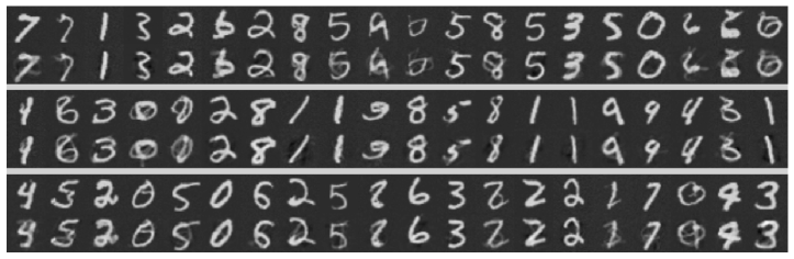
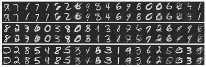
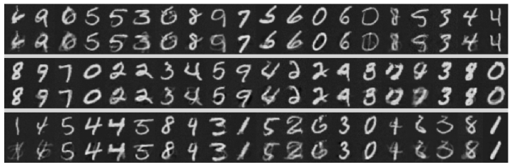
Figure 4: MNIST 32x32 image generation. Every top row is the integration of the corresponding ODE via Dormand-Prince’s $5/4$ method, which makes $108$ function evaluations. Every bottom row corresponds to single function evaluation approximation.

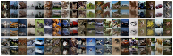
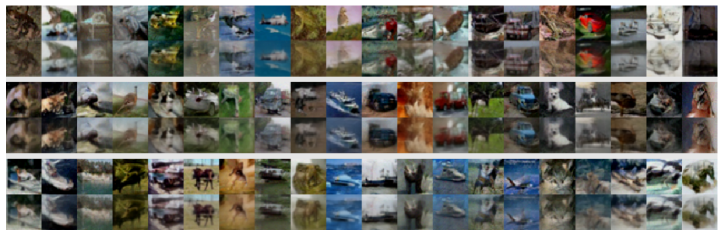
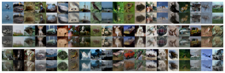
Figure 5: CIFAR-10 image generation. Every top row is the integration of the corresponding ODE via Dormand-Prince’s $5/4$ method, which makes $78$ function evaluations. Every bottom row corresponds to single function evaluation approximation.

References

• Albergo & Vanden-Eijnden (2022) Michael S Albergo and Eric Vanden-Eijnden. Building normalizing flows with stochastic interpolants. International Conference on Learning Representations, 2022.
• Albergo et al. (2023) Michael S. Albergo, Nicholas M. Boffi, and Eric Vanden-Eijnden. Stochastic interpolants: A unifying framework for flows and diffusions. arXiv preprint 2303.08797, 2023.