SWAP-type geometric gates induced by paths on Schmidt sphere

Abstract

We propose SWAP-type quantum gates based on geometric phases purely associated with paths on the Schmidt sphere [Phys. Rev. A 62, 022109 (2000)]. These geometric Schmidt gates can entangle qubit pairs to an arbitrary degree; in particular, they can create maximally entangled states from product states by an appropriate choice of base point on the Schmidt sphere. We identify Hamiltonians that generate pure paths on the Schmidt sphere by reverse engineering and demonstrate explicitly that the resulting Hamiltonians can be implemented in systems of transmon qubits. The geometric Schmidt gates are characterized by vanishing dynamical phases and are complementary to geometric single-qubit gates that take place on the Bloch sphere.

Geometric quantum computation ekert00 ; zhang23 is the idea to use Abelian geometric phases berry84 ; aharonov87 to build robust quantum gates. This has been implemented on different experimental platforms, such as nuclear magnetic resonance jones00 , trapped ions kim08 , electron spin resonance wu13 , NV centers in diamond kleissler18 , and superconducting qubits xu20 . A universal set of geometric gates requires arbitrary single-qubit gates solely dependent upon paths on the Bloch sphere, supplemented by a geometric gate that can entangle pairs of qubits zhu03 .

Realizations of two-qubit gates are particularly challenging as they are limited by the naturally occurring type of qubit-qubit interaction in the chosen system schuch03 . For instance, while entangling gates such as CNOT and controlled phase flip can be implemented using a single application of Ising interaction terms, SWAP-type entangling gates such as $i$SWAP and $\sqrt{{\rm SWAP}}$ are similarly implementable in the presence of various forms of spin exchange interactions, such as XY or Heisenberg schuch03 . As such interaction terms are common in several qubit systems tanamoto09 ; rasmussen20 , it becomes pertinent to develop schemes for geometric SWAP-type gates. Here, we propose such a general approach to geometric two-qubit gates.

The idea of our proposal is based on the Schmidt decomposition nielsen00 , i.e., that any pure bipartite state can be written on Schmidt form, being a superposition of Schmidt vectors. These vectors are products of mutually orthogonal states for each subsystem. When the two subsystems are qubits, the Schmidt decomposition can be represented on a two-dimensional ‘Schmidt sphere’ sjoqvist00 . This sphere is parametrized by a polar angle that determines the degree of qubit-qubit entanglement and an azimuthal angle that takes care of the relative phase of the Schmidt vectors. The relevance of the Schmidt sphere has been studied experimentally using polarization-entangled photon pairs loredo14 .

Here, we introduce geometric Schmidt gates that are two-qubit gates controlled by the solid angle enclosed on the Schmidt sphere. This is achieved by designing a complete set of orthonormal two-qubit states that acquire no dynamical phase and whose Schmidt vectors are kept constant throughout the implementation of the gate. These gates are the two-qubit analog of the single-qubit geometric gates associated with paths on the Bloch sphere. The geometric Schmidt gates are in a sense optimal as they require the same amount of parameter control as their single-qubit counterparts. We examine their ability to entangle the qubit pair by analyzing Makhlin’s local invariants makhlin02 . We identify the Hamiltonians that generate the gates by means of reverse engineering berry09 and demonstrate that they can be realized in systems with controllable spin exchange terms.

Consider two qubits with local Hilbert spaces $\mathscr{H}_{a}$ and $\mathscr{H}_{b}$. Any pure state belonging to $\mathscr{H}_{a}\otimes\mathscr{H}_{b}$ of the two qubits can, up to an unimportant overall phase, be written on Schmidt form nielsen00 :

$$|\Gamma_{+}({\bf r})\rangle=f|{\bf n}\rangle\otimes|{\bf m}\rangle+g|-{\bf n}\rangle\otimes|-{\bf m}\rangle,$$ (1)

where $|\pm{\bf n}\rangle$ and $|\pm{\bf m}\rangle$ are orthonormal vector pairs belonging to $\mathscr{H}_{a}$ and $\mathscr{H}_{b}$, respectively. The amplitudes $f=e^{-i\beta/2}\cos\frac{\alpha}{2}$ and $g=e^{i\beta/2}\sin\frac{\alpha}{2}$ define the angles $\alpha$ and $\beta$ that parameterize a point

$${\bf r}=(\sin\alpha\cos\beta,\sin\alpha\sin\beta,\cos\alpha)$$ (2)

on the Schmidt sphere sjoqvist00 . Note that only the polar $\alpha$ is related to the amount of entanglement, as the azimuthal angle $\beta$ can be controlled by locally manipulating one of the qubits. The Bloch vectors of the marginal states of the two qubits point along ${\bf n}$ and ${\bf m}$ in the case where $|f|\neq|g|$, while these vectors distinguish different maximally entangled states milman03 ; milman06 when $|f|=|g|$ remark1 . Thus, any two-qubit state is fully specified by the triplet $({\bf r},{\bf n},{\bf m})$ and the evolution of the system can be viewed as paths on the local Bloch spheres and the Schmidt sphere loredo14 .

In order to implement geometric Schmidt gates, we supplement $|\Gamma_{+}({\bf r})\rangle$ with the states

$$|\Gamma_{-}({\bf r})\rangle = -g^{\ast}|{\bf n}\rangle\otimes|{\bf m}\rangle+f^{\ast}|-{\bf n}\rangle\otimes|-{\bf m}\rangle,$$

$$|\Lambda_{+}\rangle = |{\bf n}\rangle\otimes|-{\bf m}\rangle,\ \ \ \ |\Lambda_{-}\rangle=|-{\bf n}\rangle\otimes|{\bf m}\rangle$$ (3)

and require ${\bf n}\equiv{\bf n}_{0}$ and ${\bf m}\equiv{\bf m}_{0}$ to be fixed throughout the implementation of the gate. Thus, the Schmidt gate scenario is the special case where the evolution path is nontrivial only on the Schmidt sphere. Provided the dynamical phases all vanish or can be factored out as an overall global phase, a loop $\mathscr{C}:[0,\tau]\ni t\mapsto{\bf r}_{t}$, ${\bf r}_{\tau}={\bf r}_{0}\equiv(\sin\alpha_{0}\cos\beta_{0},\sin\alpha_{0}\sin\beta_{0},\cos\alpha_{0})$, that encloses a solid angle $\Omega$ on the Schmidt sphere induces the geometric two-qubit gate

$${\rm U}_{\alpha_{0},\beta_{0}}(\mathscr{C})=|{\bf n}_{0}\rangle\langle{\bf n}_{0}|\otimes|-{\bf m}_{0}\rangle\langle-{\bf m}_{0}|$$

$$+|-{\bf n}_{0}\rangle\langle-{\bf n}_{0}|\otimes|{\bf m}_{0}\rangle\langle{\bf m}_{0}|+e^{-i\Omega/2}|\Gamma_{+}({\bf r}_{0})\rangle\langle\Gamma_{+}({\bf r}_{0})|$$

$$+e^{i\Omega/2}|\Gamma_{-}({\bf r}_{0})\rangle\langle\Gamma_{-}({\bf r}_{0})|.$$ (4)

This is the desired geometric Schmidt gate whose action is controlled by $\Omega$ enclosed by the loop $\mathscr{C}$ on the Schmidt sphere.

The ability of ${\rm U}_{\alpha_{0},\beta_{0}}(\mathscr{C})$ to entangle the qubit pair relies on the base point ${\bf r}_{0}$ on the Schmidt sphere. To see this, let us consider two extreme cases: (i) ${\bf r}_{0}=(0,0,1)$ and (ii) ${\bf r}_{0}=(0,1,0)$. We shall see that while (i) cannot entangle, (ii) contains, up to a rotation around the $z$ axis, the only special perfect entangler rezakhani04 , i.e., the only geometric Schmidt gate that can create maximally entangled states from an orthonormal basis of product states. In the following, we put ${\bf n}_{0}=-{\bf m}_{0}=(0,0,1)$ such that $|{\bf n}_{0}\rangle=|0\rangle$ and $|{\bf m}_{0}\rangle=|1\rangle$, as well as use short-hand notation $|xy\rangle\equiv|x\rangle\otimes|y\rangle$, $x,y=0,1$, and $AB\equiv A\otimes B$ for operators $A$ and $B$ acting on $\mathscr{H}_{a}$ and $\mathscr{H}_{b}$, respectively.

In case (i), we find

$${\rm U}^{(i)}(\mathscr{C}) \equiv {\rm U}_{0,0}(\mathscr{C})=|00\rangle\langle 00|+|11\rangle\langle 11|$$ (5)

$$+e^{-i\Omega/2}|01\rangle\langle 01|+e^{i\Omega/2}|10\rangle\langle 10|,$$

whose action on a generic two-qubit state $|\psi\rangle=a|00\rangle+b|01\rangle+c|10\rangle+d|11\rangle$ results in the transformation

$$|\psi\rangle\mapsto|\tilde{\psi}\rangle = a|00\rangle+e^{-i\Omega/2}b|01\rangle+e^{i\Omega/2}c|10\rangle+d|11\rangle.$$ (6)

This clearly preserves concurrence wootters98 : ${\rm C}(\psi)=2|ad-bc|\mapsto{\rm C}(\tilde{\psi})=2|ad-be^{-i\Omega/2}ce^{i\Omega/2}|=2|ad-bc|$. Thus, ${\rm U}^{(i)}(\mathscr{C})$ cannot entangle the qubits.

In case (ii), we instead have

$${\rm U}^{(ii)}(\mathscr{C}) \equiv {\rm U}_{\frac{\pi}{2},\frac{\pi}{2}}(\mathscr{C})=|00\rangle\langle 00|+|11\rangle\langle 11|$$ (7)

$$+e^{-i\Omega/2}|\Psi_{+}\rangle\langle\Psi_{+}|+e^{i\Omega/2}|\Psi_{-}\rangle\langle\Psi_{-}|$$

with the maximally entangled states $|\Psi_{\pm}\rangle=\frac{1}{\sqrt{2}}\big{(}|01\rangle\pm i|10\rangle\big{)}$, yielding

$${\rm U}^{(ii)}(\mathscr{C})=\left(\begin{array}[]{cccc}1&0&0&0\\ 0&\cos\frac{\Omega}{2}&-\sin\frac{\Omega}{2}&0\\ 0&\sin\frac{\Omega}{2}&\cos\frac{\Omega}{2}&0\\ 0&0&0&1\\ \end{array}\right)$$ (12)

expressed in the computational basis $\{|00\rangle,|01\rangle,|10\rangle,|11\rangle\}$.

To analyze the entangling capacity of ${\rm U}^{(ii)}(\mathscr{C})$, we calculate Makhlin’s local invariants $G_{1}$ and $G_{2}$ for a two-qubit gate ${\rm U}$ makhlin02 . These are found by the following procedure. First, introduce the unitary operator ${\rm Q}=|B_{1}\rangle\langle 00|+|B_{2}\rangle\langle 01|+|B_{3}\rangle\langle 10|+|B_{4}\rangle\langle 11|$ that transforms the computational basis into the Bell basis $|B_{1}\rangle=\frac{1}{\sqrt{2}}(|00\rangle+|11\rangle)$, $|B_{2}\rangle=\frac{i}{\sqrt{2}}(|01\rangle+|10\rangle)$, $|B_{3}\rangle=\frac{1}{\sqrt{2}}(|01\rangle-|10\rangle)$, and $|B_{4}\rangle=\frac{i}{\sqrt{2}}(|00\rangle-|11\rangle)$. Second, define $m=\left({\rm Q}^{\dagger}{\rm U}{\rm Q}\right)^{\rm T}{\rm Q}^{\dagger}{\rm U}{\rm Q}$, in terms of which the local invariants are found as

$$G_{1} = \frac{\text{Tr}^{2}m}{16\det U},$$

$$G_{2} = \frac{\text{Tr}^{2}m-\text{Tr}m^{2}}{4\det U},$$ (13)

where the latter is real-valued makhlin02 .

Necessary and sufficient conditions for a perfect entangler (PE) that can maximally entangle a product state are $0\leq\left|G_{1}\right|\leq\frac{1}{4}$ and $-1\leq G_{2}\leq 1$ balakrishnan10 ; a special perfect entangler (SPE) rezakhani04 , which is a gate that maximally entangles an orthonormal product basis, is such that $G_{1}=0$ and $-1\leq G_{2}\leq 1$. The SPEs saturate the upper bound $\frac{2}{9}$ of the entangling power for qubit pairs zanardi00 . Direct calculation for ${\rm U}={\rm U}^{(ii)}(\mathscr{C})$ yields

$$G_{1} = \cos^{4}\frac{\Omega}{2},$$

$$G_{2} = 1+2\cos\Omega.$$ (14)

We thus see that we can only find PEs for solid angles $\frac{\pi}{2}\leq\left|\Omega\right|\leq\pi$ with the upper bound corresponding to an SPE. In fact, for $\Omega=-\pi$, one finds the SWAP-type gate:

$${\rm U}^{(ii)}(\mathscr{C})=\left(\begin{array}[]{cccc}1&0&0&0\\ 0&0&1&0\\ 0&-1&0&0\\ 0&0&0&1\\ \end{array}\right),$$ (19)

which is an SPE that maximally entangles the orthonormal product states $\frac{1}{2}(|0\rangle\pm|1\rangle)\otimes(|0\rangle\pm|1\rangle)$ and $\frac{1}{2}(|0\rangle\pm|1\rangle)\otimes(|0\rangle\mp|1\rangle)$.

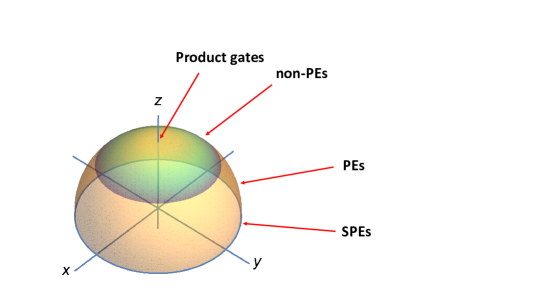
Figure 1: Entangling capacity on the Schmidt sphere. Perfect entanglers (PEs) are loops based at points with polar angles $\alpha_{0}\in[\frac{\pi}{4},\frac{\pi}{2}]$ with the special perfect entanglers (SPEs) on the equator $\alpha_{0}=\frac{\pi}{2}$. There are no product states that can be transformed into a maximally entangled state by gates for base points with $\alpha_{0}\in[0,\frac{\pi}{2})$. Product gates, such as ${\rm U}^{(i)}(\mathscr{C})$ in Eq. (5), are located at the north pole. While we show only the upper half for clarity, exactly the same classification of gates can be found on the lower half of the Schmidt sphere.

We next analyze which base points ${\bf r}_{0}$ on the Schmidt sphere allows for PEs. For the general ${\rm U}_{\alpha_{0},\beta_{0}}(\mathscr{C})$, we find the local invariants

$$G_{1} = \frac{1}{16}\left[4-2\sin^{2}\alpha_{0}\left(1-\cos\Omega\right)\right]^{2},$$

$$G_{2} = 3-2\sin^{2}\alpha_{0}\left(1-\cos\Omega\right),$$ (20)

which confirms that the azimuthal angle $\beta_{0}$ is irrelevant to the entangling capacity, as noted before. We see that there are no PEs for $\alpha_{0}\in[0,\frac{\pi}{4})$. We also see that $G_{1}\geq\cos^{4}\alpha_{0}$, which implies that ${\rm U}_{\alpha_{0},\beta_{0}}(\mathscr{C})$ can be an SPE only for base points on the equator $\alpha_{0}=\frac{\pi}{2}$.

In the general case, not only $|\Gamma_{\pm}\rangle\in{\rm Span}\{|01\rangle,|10\rangle\}$ but also $\Lambda_{\pm}\in{\rm Span}\{|00\rangle,|11\rangle\}$ can evolve purely on the Schmidt sphere. As the two pairs $|\Gamma_{\pm}\rangle$ and $|\Lambda_{\pm}\rangle$ evolve in orthogonal subspaces, such gates factorize into products of commuting geometric Schmidt gates:

$${\rm U}_{\alpha_{0}^{\prime},\beta_{0}^{\prime};\alpha_{0},\beta_{0}}(\mathscr{C^{\prime}},\mathscr{C}) = {\rm U}_{\alpha_{0}^{\prime},\beta_{0}^{\prime}}(\mathscr{C}^{\prime}){\rm U}_{\alpha_{0},\beta_{0}}(\mathscr{C}),$$

$$\left[{\rm U}_{\alpha_{0}^{\prime},\beta_{0}^{\prime}}(\mathscr{C}^{\prime}),{\rm U}_{\alpha_{0},\beta_{0}}(\mathscr{C})\right] = 0.$$ (21)

Here,

$${\rm U}_{\alpha_{0}^{\prime},\beta_{0}^{\prime}}(\mathscr{C}^{\prime}) = |01\rangle\langle 01|+|10\rangle\langle 10|$$ (22)

$$+e^{-i\Omega^{\prime}/2}|\Lambda_{+}({\bf r}_{0}^{\prime})\rangle\langle\Lambda_{+}({\bf r}_{0}^{\prime})|$$

$$+e^{i\Omega^{\prime}/2}|\Lambda_{-}({\bf r}_{0}^{\prime})\rangle\langle\Lambda_{-}({\bf r}_{0}^{\prime})|$$

with

$$|\Lambda_{+}({\bf r}_{0}^{\prime})\rangle = e^{-i\beta_{0}^{\prime}/2}\cos\frac{\alpha_{0}^{\prime}}{2}|00\rangle+e^{i\beta_{0}^{\prime}/2}\sin\frac{\alpha_{0}^{\prime}}{2}|11\rangle,$$

$$|\Lambda_{-}({\bf r}_{0}^{\prime})\rangle = -e^{-i\beta_{0}^{\prime}/2}\sin\frac{\alpha_{0}^{\prime}}{2}|00\rangle+e^{i\beta_{0}^{\prime}/2}\cos\frac{\alpha_{0}^{\prime}}{2}|11\rangle.$$ (23)

Thus, the only essential difference between ${\rm U}_{\alpha_{0}^{\prime},\beta_{0}^{\prime}}(\mathscr{C}^{\prime})$ and ${\rm U}_{\alpha_{0},\beta_{0}}(\mathscr{C})$ is that the former couples $|00\rangle$ and $|11\rangle$, while the latter couples $|01\rangle$ and $|10\rangle$); in other words, their entangling capacity is the same and thus for both captured by the above analysis.

We now examine the physical realization of the geometric Schmidt gates. We focus on the case where only Schmidt vectors in ${\rm Span}\{|01\rangle,|10\rangle\}$ evolve and where ${\bf n}_{0}=-{\bf m}_{0}=(0,0,1)$. Thus, we look for the Hamiltonian that generates the time dependent Schmidt vectors

$$|\Gamma_{+}({\bf r}_{t})\rangle = f(t)|01\rangle+g(t)|10\rangle,$$

$$|\Gamma_{-}({\bf r}_{t})\rangle = -g^{\ast}(t)|01\rangle+f^{\ast}(t)|10\rangle,$$

$$|\Lambda_{+}\rangle = |00\rangle,\ \ \ |\Lambda_{-}\rangle=|11\rangle.$$ (24)

To this end, we insert the ansatz

$$H(t) = \omega_{22}(t)\,|01\rangle\langle 01|+\omega_{33}(t)\ |10\rangle\langle 10|$$ (25)

$$+\omega_{23}(t)|01\rangle\langle 10|+{\rm H.c.}$$

and Eq. (24) into the Schrödinger equation, yielding ($\hbar=1$ from now on)

$$i\dot{f} = \omega_{22}f+\omega_{23}g,\ \ \ i\dot{g}=\omega_{23}^{\ast}f+\omega_{33}g,$$

$$-i\dot{g}^{\ast} = -\omega_{22}g^{\ast}+\omega_{23}f^{\ast},\ \ \ i\dot{f}^{\ast}=-\omega_{23}^{\ast}g^{\ast}+\omega_{33}f^{\ast}.$$ (26)

These equations have the solution

$$\omega_{22} = -\omega_{33}=i\left(\dot{f}f^{\ast}+g\dot{g}^{\ast}\right),$$

$$\omega_{23} = i\left(\dot{f}g^{\ast}-f\dot{g}^{\ast}\right),$$ (27)

where we have used that $|f|^{2}+|g|^{2}=1$, which in turn implies that $\dot{f}f^{\ast}+g\dot{g}^{\ast}$ is purely imaginary, ensuring that $\omega_{22}$ and $\omega_{33}$ are real-valued. By using the parametrization $f=e^{-i\beta/2}\cos\frac{\alpha}{2}$ and $g=e^{i\beta/2}\sin\frac{\alpha}{2}$, we find

$$\omega_{22}=-\omega_{33}=\frac{\dot{\beta}}{2},\ \ \ \omega_{23}=-\frac{\dot{\alpha}}{2}(\sin\beta+i\cos\beta).$$ (28)

We can use the identities $|0\rangle\langle 0|=\frac{1}{2}(\hat{1}+{\rm Z})$, $|1\rangle\langle 1|=\frac{1}{2}(\hat{1}-{\rm Z})$, $|0\rangle\langle 1|=\frac{1}{2}({\rm X}+i{\rm Y})$, and Eq. (28) to derive the reverse engineered Hamiltonian

$$H=-\frac{\dot{\alpha}}{2}\sin\beta\ h_{\rm XY}+\frac{\dot{\alpha}}{2}\cos\beta\ h_{\rm DM}+\frac{\dot{\beta}}{2}\ h_{\rm Z},$$ (29)

where we have identified the XY, Dzyaloshinskii–Moriya (DM), and Zeeman terms:

$$h_{\rm XY} = \frac{1}{2}\Big{(}{\rm X}{\rm X}+{\rm Y}{\rm Y}\Big{)},\ \ \ h_{\rm DM}=\frac{1}{2}\Big{(}{\rm Y}{\rm X}-{\rm X}{\rm Y}\Big{)},$$

$$h_{\rm Z} = \frac{1}{2}\Big{(}{\rm Z}\hat{1}-\hat{1}{\rm Z}\Big{)},$$ (30)

respectively. One can verify that these operators satisfy the standard SU(2) algebra: $[h_{\rm XY},h_{\rm DM}]=2ih_{\rm Z}$ with cyclic permutations. Thus, $H$ in Eq. (29) describes an effective ‘spin-$\frac{1}{2}$’ ${\bf S}\equiv\frac{1}{2}(h_{\rm XY},h_{\rm DM},h_{\rm Z})$ interacting with an effective ‘magnetic field’ ${\bf B}\equiv(\dot{\alpha}\sin\beta,\dot{\alpha}\cos\beta,\dot{\beta})$.

The paths generated by $H$ are controlled by only two parameters and give rise to geometric gates provided the dynamical phases vanish. The latter can be assured most easily by following a pair of geodesic segments forming a loop on the Schmidt sphere, in analogy with the orange-slice-paths on the Bloch sphere used to implement geometric single-qubit gates thomas11 ; zhao17 ; zhou21 .

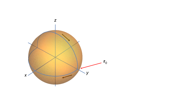
Figure 2: Orange-slice curve on the Schmidt sphere that implements the perfect entangler ${\rm U}^{(ii)}(\mathscr{C})$ in Eq. (19). The curve starts and ends at ${\bf r}_{0}=(0,1,0)$ and consists of two path segments generated by sequentially applying Zeeman and XY interactions to the qubit pair. The enclosed solid angle is $-\pi$.

We illustrate this latter point by demonstrating a realization of the SWAP-type gate ${\rm U}^{(ii)}(\mathscr{C})$ in Eq. (19). A geometric implementation of this gate is obtained by traversing an orange-slice path on the Schmidt sphere that connects the points ${\bf r}_{0}=(0,1,0)$ and ${\bf r}_{t_{1}}=(0,-1,0)$ along the equator and thereafter back along a geodesic through the north pole:

$$t \in [0,\tau]\mapsto{\bf r}_{t}$$ (33)

$$= \left\{\begin{array}[]{cl}\left[\sin\left(\pi\frac{t}{t_{1}}\right),\cos\left(\pi\frac{t}{t_{1}}\right),0\right],&0\leq t\leq t_{1},\\ \left[0,\cos\left(\pi\frac{t-t_{1}}{\tau-t_{1}}\right),\sin\left(\pi\frac{t-t_{1}}{\tau-t_{1}}\right)\right],&t_{1}\leq t\leq\tau,\end{array}\right.$$

thereby enclosing a solid angle $-\pi$, see Fig. 2. This is achieved by applying the two-pulse Hamiltonian

$$H(t)=\left\{\begin{array}[]{cl}-\frac{\pi}{2t_{1}}\ h_{\rm Z},&0\leq t\leq t_{1},\\ -\frac{\pi}{2\left(\tau-t_{1}\right)}\ h_{\rm XY},&t_{1}\leq t\leq\tau.\end{array}\right.$$ (36)

Our scheme is implementable in any qubit system that naturally include XY and DM spin exchange interaction. Specifically, the above path that generates ${\rm U}^{(ii)}(\mathscr{C})$ can be realized for two transmon qubits coupled by a transmssion line on a chip majer07 . Here, the first Zeeman pulse in Eq. (36) is generated by detuning the qubits by an amount $\pm\delta=\mp\frac{1}{2t_{1}}$, respectively, from their idle frequencies salathe15 , while the second pulse is realized via exchange of virtual photons in the cavity by tuning the transition frequencies of the two transmon qubits into resonance majer07 . In this way, one takes advantage of the naturally occuring XY interaction term for direct implemention of the geometric SWAP-type gate in Eq. (19).

Realization of more general paths in the transmon setting would require simultaneous applications of the XY and Zeeman terms. To achieve this, one may use Suzuki-Trotter-based techniques lloyd96 to simulate the effect of such spin models salathe15 . For instance, by performing the second path segment so as to make an angle $\theta$ to the $yz$ plane would require application of the Hamiltonian

$$H_{\theta}(t)=-\frac{\pi}{2\left(\tau-t_{1}\right)}\left(\cos\theta\ h_{\rm XY}-\sin\theta\ h_{\rm Z}\right),\ \ t_{1}\leq t\leq\tau,$$ (37)

which implements ${\rm U}^{(ii)}(\mathscr{C})$ in Eq. (12) with $\Omega=2\theta$. This can be simulated by performing

$$U_{n}=e^{i\frac{\pi}{2n}\cos\theta\ h_{\rm XY}}e^{-i\frac{\pi}{2n}\sin\theta\ h_{\rm Z}}$$ (38)

$n$ times. In this way, the solid angle dependence of the gate can be tested by varying $\theta$.

To complete a universal set, one needs to implement sufficiently flexible single-qubit gates. One may achieve this by means of paths on the local Bloch spheres, while keeping the Schmidt parameters $\alpha,\beta$ fixed. These gates can be assured to be geometric by designing the paths so that the dynamical phases all vanish, for instance by using geodesic segments on the Bloch spheres. Thus, by generating ordered sequences of paths on Schmidt and Bloch spheres, any quantum computation can be realized efficiently by purely geometric means.

In conclusion, we have demonstrated a class of two-qubit gates associated with paths on the Schmidt sphere. These gates control the entangling capacity of the two-qubit evolution and have a clear geometric interpretation in terms of solid angles enclosed on the Schmidt sphere. A key point of our proposal is that it provide means for experimentally implementing SWAP-type geometric gates based on spin exchange terms that naturally appear in several qubit architectures.

References

(1) A. Ekert, M. Ericsson, P. Hayden, H. Inamori, J. A. Jones,
D. K. L. Oi, and V. Vedral,