Fast quantum control of cavities using an improved protocol without coherent errors

Abstract

The selective number-dependent arbitrary phase (SNAP) gates form a powerful class of quantum gates, imparting arbitrarily chosen phases to the Fock modes of a cavity. However, for short pulses, coherent errors limit the performance. Here we demonstrate in theory and experiment that such errors can be completely suppressed, provided that the pulse times exceed a specific limit. The resulting shorter gate times also reduce incoherent errors. Our approach needs only a small number of frequency components, the resulting pulses can be interpreted easily, and it is compatible with fault-tolerant schemes.

The field of circuit quantum electrodynamics (cQED) [1] employs microwave cavities coupled to superconducting qubits and defines one of the most promising platforms for quantum computation. Modern 3D cavities offer long coherence times up to milliseconds [2] and beyond [3, 4]. This provides the opportunity to store and process the quantum information in the bosonic modes of the cavity. The strong coupling to the superconducting qubit allows fast and flexible manipulation of the cavity’s quantum state. These setups showed remarkable success in realizing arbitrary operations on quantum systems for quantum simulations [5] or implementing bosonic quantum error correction [6, 7, 8, 9], even reaching the so-called break-even point.

Two different approaches exist to gain universal control over the cavity-qubit system. For the first one, cavity and qubit are driven simultaneously with pulse sequences that are typically numerically optimized [10], e.g. with GRAPE [11], to approximate a certain unitary operation. The second approach uses the powerful selective number-dependent arbitrary phase (SNAP) gate, which can impart any desired set of phases on the Fock modes of the cavity [12]. For example, with cavity displacements, the SNAP gate can be easily extended to a universal gate set, for which [13, 14] provide efficient schemes to approximate any desired unitary. Because any errors accumulate in such sequences, it is crucial to improve the fidelity of an individual SNAP gate as far as possible to enable the realization of more complex unitaries.

To both avoid incoherent errors and ensure a rapid overall processing speed, it is desirable to make the SNAP gate time as short as possible. However, in that regime, the fidelity suffers from coherent errors.

To overcome this challenge, recently numerical techniques were employed to optimize the envelope of the SNAP pulses, providing fast SNAP gates and enable the preparation of arbitrary cavity states with high fidelity [15]. However, numerical optimization schemes, like [15] or using GRAPE [10, 11], tend to have thousands of adjustable parameters, are thus hard to interpret, and incorporate high-frequency components. In our work, we present a simple approach which, above some pulse duration, can completely suppress the coherent errors based on a geometrical interpretation of the errors. Our optimized pulses are continuous in time and preserve the original form of the SNAP gate pulses [12] without introducing additional frequencies. We demonstrate experimentally that our pulses reduce the excited state error of the SNAP gate, the dominant coherent error, by $53\text{\,}\mathrm{\char 37\relax}$ compared to the best vanilla SNAP gate protocol for realistic target operations. Additionally, our optimization is compatible with the fault-tolerant scheme of [16, 17, 18] that aims to suppress incoherent errors, and both approaches combined yield higher fidelities than each of them individually.

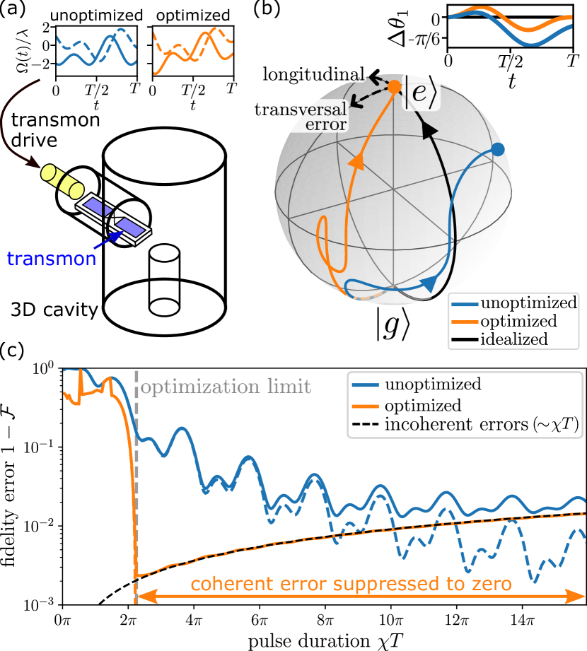
Figure 1: Experimental setup and principle of our optimization scheme. (a) Circuit QED platform: a transmon (blue) is coupled to a 3D microwave cavity and a readout resonator (yellow). By driving the transmon with a slow pulse $\Omega(t)$ (solid lines: $\real(\Omega(t))$, dashed lines: $\imaginary(\Omega(t)))$, the target phase shifts are applied selectively to the Fock modes of the cavity, implementing the first stage of the SNAP gate. Our scheme improves (orange) the unoptimized (blue) pulse sequences in Eq. 3 by adapting the amplitudes, frequencies and phases of the individual drive terms. (b) Simulated coherent time evolution for one selected Fock mode [here $n=1$ with $\Delta\theta_{1}(t)=\arg(\bra{g,1}\ket{\psi(t)})-\theta_{1}$, $\chi T=2.25\pi$, and $\vec{\theta}=(0,-\pi/4,\pi/2)$]. The evolution under the unoptimized pulse (blue) deviates from the ideal trajectory (black), resulting in a coherent error. For the optimized pulse (orange) the evolution still deviates, but reaches the target state. The corresponding pulse sequences are shown in (a). (c) Total SNAP gate fidelity error (solid lines) as function of the pulse duration. For unoptimized pulses, the coherent error (dashed blue) decreases for larger pulse durations and vanishes in the limit $\chi T\to\infty$, but the incoherent error (dashed black, analytical approximation, for derivation see Appendix F) increases with the pulse duration $\sim\chi T$. Our scheme reduces the coherent error to zero above the optimization limit (gray).

We perform our experiments in a cQED setup consisting of a 3D storage cavity which is dispersively coupled to a transmon qubit [19] (see Fig. 1(a)) to manipulate the state in the cavity. Moreover, the transmon is coupled to a readout resonator to measure the transmon state and to drive the transmon. The readout will not be included in our description of the system (see Appendix H for a summary of the concrete system parameters). Initially, the transmon is prepared in the ground state, and the cavity can be in an arbitrary state. Our SNAP gate consists of two stages: In the first stage, a slow and selective $\pi$ pulse is applied to excite the transmon and to apply the target phase shifts $\vec{\theta}$ to the respective Fock modes. The $\pi$ pulse of the second stage is fast and so unselective and just brings the transmon back into the ground state. Ideally, this implements the SNAP gate:

$$\mathrm{SNAP}(\vec{\theta})=\sum_{n}\mathrm{e}^{\mathrm{i}\theta_{n}}\outerproduct{n}{n}$$ (1)

on the cavity.

However, the selectiveness of the first stage is only given in the limit of large pulse durations resulting in incoherent errors, while shorter pulses lead to coherent errors. In contrast, the second stage is almost error-free and will not be addressed by our optimization scheme. In the following, we discuss how the coherent errors of the first stage can be classified and how our optimization scheme deals with them.

In the dispersive coupling limit, the Hamiltonian of the cavity-transmon system can be written as [19, 13, 12]:

$$\hat{H}=\hat{H}_{0}+\hat{H}_{\chi}+\hat{H}_{\mathrm{drive}}$$ (2)

with $\hat{H}_{0}=\omega_{c}\hat{a}^{\dagger}\hat{a}+\omega_{ge}\outerproduct{e}{e}$ as the cavity and transmon energy, $\hat{H}_{\chi}=-\chi\outerproduct{e}{e}\hat{a}^{\dagger}\hat{a}$ as the dispersive coupling between both and $\hat{H}_{\mathrm{drive}}=\Omega(t)\mathrm{e}^{-\mathrm{i}\omega_{ge}t}\outerproduct{e}{g}+\mathrm{H.c.}$ as the transmon drive. $\omega_{ge}$ is the transition frequency between the first two transmon states $\ket{g}$ and $\ket{e}$, $\omega_{c}$ the cavity frequency, $\chi$ the dispersive coupling frequency, $\hat{a}$/$\hat{a}^{\dagger}$ the destruction/creation operator of a cavity excitation and $\Omega(t)$ the pulse envelope applied on the transmon. For simplicity, we work in the following in the frame rotating with $\hat{H}_{0}+\hat{H}_{\chi}$. Note that for practical applications, also higher order contributions to Eq. 2 have to be considered, like the Kerr term $-(K/2)\hat{a}^{{\dagger}^{2}}\hat{a}^{2}$ and the correction to the dispersive coupling $(\chi^{\prime}/2)\outerproduct{e}{e}\hat{a}^{{\dagger}^{2}}\hat{a}^{2}$ [12], which are further discussed in Appendix D.

The input state can be expanded in the Fock space as $\ket{\psi_{\mathrm{in}}}=\sum_{n}c_{n}\ket{gn}$ with $\vec{c}$ as the normalized and complex amplitude vector. As our Hamiltonian in Eq. 2 conserves the photon number, the amplitude vector is time independent, while the initial $\ket{gn}$ states evolve in time. During the first stage, the pulse function of the unoptimized SNAP protocol [12, 13]

$$\Omega_{\mathrm{unopt}}(t)=\lambda\sum_{n}\mathrm{e}^{\mathrm{i}(\chi nt+\theta_{n})}$$ (3)

is applied with $\lambda=\pi/(2T)$ as the unoptimized pulse amplitude and $T$ as the pulse duration. Each of the terms aims to resonantly drive the corresponding transition $\ket{gn}\leftrightarrow\ket{en}$. In the limit $T\gg 1/\chi$ (see Appendix A), for each Fock mode the coherent time evolution follows a perfect half circle on the Bloch sphere and reaches the target state $\ket{\psi_{\mathrm{target}}(\vec{c})}=\sum_{n}c_{n}\mathrm{e}^{\mathrm{i}\theta_{n}}\ket{en}$ (see Fig. 1(b)). However, for finite pulse durations counter-rotating terms have to be taken into account. Thus, the actual trajectories differ and the final states deviate for each Fock mode from the target ones in the following three ways: (i) the acquired phases are shifted by the phase errors $\Delta\theta_{n}$, (ii) on the Bloch sphere the trajectories overshoot or stop too early, here denoted as the longitudinal errors $\epsilon_{n}^{(L)}$, and (iii) the end points on the Bloch sphere deviate perpendicular to the orientation of the ideal trajectory, labeled as the transversal errors $\epsilon_{n}^{(T)}$. In general, the actual final state is given with these three error contributions as (see Appendix B):

$$\ket{\psi_{\mathrm{out}}(\vec{c})}=$$

$$\qquad\sum_{n}c_{n}\Bigg{(}\sqrt{1-\frac{\absolutevalue{\epsilon_{n}}^{2}}{4}}\mathrm{e}^{\mathrm{i}(\theta_{n}+\Delta\theta_{n})}\ket{en}-\frac{\epsilon_{n}}{2}\ket{gn}\Bigg{)}$$ (4)

with $\epsilon_{n}=(\epsilon_{n}^{(L)}+\mathrm{i}\epsilon_{n}^{(T)})\mathrm{e}^{\mathrm{i}\Delta\theta_{n}}$.

To compensate these errors, we modify the pulse sequence of Eq. 3 in the following way:

$$\Omega_{\mathrm{opt}}(t)=\sum_{n}\lambda_{n}\mathrm{e}^{\mathrm{i}(\omega_{n}t+\alpha_{n}-\Delta\omega_{n}T/2)}$$ (5)

with $\lambda_{n}$, $\omega_{n}$ and $\alpha_{n}$ as the Fock level dependent amplitudes, frequencies and phases of the drive. $\Delta\omega_{n}=\omega_{n}-\chi n$ is the detuning with respect to the unoptimized frequencies of Eq. 3. The phase $-\Delta\omega_{n}T/2$ corrects an unwanted phase shift created by the detuning. In summary, we have for each Fock mode three coherent error contributions and also three correction parameters with which we want to control and correct all errors. Using first order perturbation theory in the limit of large gate times and small coherent errors, the latter can be corrected by modifying the pulse parameters by (see Supplemental Material Appendix C):

$$\Delta\lambda_{n}=-\frac{\epsilon_{n}^{(L)}}{2T};\quad\Delta\omega_{n}=\frac{\pi\epsilon_{n}^{(T)}}{2T};\quad\Delta\alpha_{n}=-\Delta\theta_{n}$$ (6)

Thus, each of the coherent errors is controlled individually by one pulse parameter.

However, for finite gate times and correspondingly large coherent errors, higher order contributions to Eq. 6 become important and the updated pulses still lead to coherent errors. To overcome this problem, we iteratively reapply Eq. 6. First, we simulate the coherent time evolution with the current pulse parameters and extract the coherent errors. Next, we update the pulse parameters according to Eq. 6. To prevent overshooting, the updates are scaled by a learning rate $\eta\in(0,1]$. This routine is repeated until the convergence fails or the coherent mean overlap error is smaller than a threshold, typically $10^{-5}$, where it is experimentally negligible. Therefore, our scheme is able to correct coherent errors far beyond the range of validity of the first order perturbation theory. In Fig. 1(b), the time evolution under the optimized pulse is compared against the vanilla SNAP gate and the ideal trajectory. At intermediate times, the counter-rotating terms still lead to a deviation from the ideal trajectory; however, the desired target state is reached nevertheless.

To quantify the overall performance of the first SNAP pulse, we define the fidelity as the mean squared overlap:

$$\mathcal{F}=\underset{\begin{subarray}{c}\vec{c}\text{ s.t.}\\ \norm{c}=1\end{subarray}}{\mathrm{avg}}\bra{\psi_{\mathrm{target}}(\vec{c})}\hat{\rho}_{\mathrm{out}}(\vec{c})\ket{\psi_{\mathrm{target}}(\vec{c})}$$ (7)

where the average covers all possible initial cavity states. $\hat{\rho}_{\mathrm{out}}(\vec{c})$ is the density matrix of the cavity-transmon system after the first stage of the SNAP gate and equals $\ket{\psi_{\mathrm{out}}(\vec{c})}\bra{\psi_{\mathrm{out}}(\vec{c})}$ if only the coherent dynamics are considered.

In Fig. 1(c), the overall performance of the SNAP gate is shown. The coherent errors of the unoptimized SNAP gate decay with increasing gate time (scaling with $1/(\chi T)^{2}$, see Appendix F), while the incoherent errors rise with the gate time (scaling with $\chi T$). Thus, the unoptimized SNAP gate is ideally operated at intermediate gate times. In contrast, our optimized pulses completely suppress coherent errors provided that the gate time exceeds a certain threshold, which we denote the ”optimiziation limit”. This limit depends on the actual target operation. Thus, our optimized SNAP gates reach their best performance at the optimization limit.

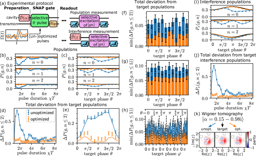
Figure 2: Experimental results, showing performance improvements for the optimized SNAP pulse sequences. (a) Experimental procedure: state preparation, SNAP gate, and readout. After the SNAP gate, we measure the populations $P(g,n)$ (top right), or extract the coherences via an interference measurement (bottom right) yielding $P_{\epsilon}(g,n)$ after a small displacement $\epsilon$. Measurement symbols indicate a dispersive readout of the qubit state via the readout resonator. (b,c) Photon-number-dependent ground state population $P(g,n)$ as function of the pulse duration (b) and target operation phase $\theta$ (c). The unoptimized (blue) and optimized (orange) pulses (dots: experiment) are compared to the ideal populations $P_{\mathrm{ideal}}(g,n)$ (black) for an error-free SNAP gate (black). Simulation results (solid) are obtained from a Lindblad master equation (see Section E.2). The statistical measurement error is smaller than the size of the points. (d, e) Total deviation $\Delta P(g,n\leq n_{\mathrm{max}})$ between the ideal and the observed populations for all Fock modes that are part of the target operation. The encircled points in (d) mark the best performance of the unoptimized and optimized SNAP gate. (f–h) Smallest total deviation with respect to the gate time for various target operations. (i, j) Populations resulting from the interference measurement with $\epsilon=0.1$ and their total deviations from their ideal values as function of the target operation phase $\theta$ (i) and as function of the pulse duration (j). (k) Wigner tomography of the cavity state after the SNAP gate was applied, compared to the desired target state. The contour line of the target state for $\mathrm{parity}=0$ is shown in gray in all 3 insets.
Considered target operations: $(0,\pi,0)$ in (b, d, j), $(0,\theta,0)$ in (c, e, f, i), $(0,\theta,0,\theta,0,\theta)$ in (g), $(0,\varphi,\theta,0,\pi,0)$ in (h), and $(0,\frac{2}{3}\pi,\pi,0,\pi,0)$ in (k). Considered gate times: $\chi T=2.5\pi$ in (c, e, i), and $\chi T=2\pi$ in (k). Considered initial coherent states: $\alpha=1.0$ in (b–f, h–j), $\alpha=1.4$ in (g), and $\alpha=0.15-0.98\mathrm{i}$ in (k).

To showcase the potential of our approach in the experiment, we first prepare the cavity in a coherent state of amplitude $\alpha$ (see Fig. 2(a)), using a displacement operation $\mathcal{\hat{D}}$. We then apply the SNAP gate, comparing the optimized and unoptimized pulse sequences for a certain target operation $\vec{\theta}$.

To determine the quality of the gate, we perform two different kinds of measurements on the final state. First, we determine the populations of the cavity-transmon system $P(g,n)$. To that end, we first measure the transmon, obtaining $P(g)$ and $P(e)$. Afterwards, the transition $\ket{gn}\leftrightarrow\ket{en}$ for a chosen Fock mode $n$ is driven selectively. A subsequent measurement of the transmon provides the Fock mode occupancies $P(n|g/e)$ conditioned on the first readout result. The resulting populations $P(g,n)$ are directly linked to the longitudinal and transversal errors defined in Fast quantum control of cavities using an improved protocol without coherent errors. If noise is neglected, they equal $\absolutevalue{c_{n}}^{2}(1-\absolutevalue{\epsilon_{n}}^{2}/4)$.

Second, to get information about the phase errors, we apply a small displacement with $\varepsilon=0.1$ to the final cavity state and measure again the populations of the cavity-transmon system, labeled as $P_{\varepsilon}(g,n)$. Due to the small displacement, neighboring Fock state components interfere and the resulting populations depend on the phase shifts acquired during the SNAP gate operation [12]. Ideally, the resulting populations in first order of $\epsilon$ equal:

$$\begin{split}P_{\mathrm{ideal},\epsilon}(g,n)=&\absolutevalue{c_{n}}^{2}+2\epsilon c_{n}c_{n-1}\sqrt{n}\cos(\theta_{n}-\theta_{n-1})\\ &-2\epsilon c_{n}c_{n+1}\sqrt{n+1}\cos(\theta_{n}-\theta_{n+1})\end{split}$$ (8)

In Fig. 2(b), our optimized pulses are compared against the standard SNAP gate, where the target was to apply a phase shift of $\pi$ to the first Fock mode while leaving the other Fock modes untouched. As intended, our optimization scheme minimizes individually for each Fock mode the deviation from the ideal ground state population. Comparing the smallest total deviations $\Delta P(g,n\leq 2)=\sum_{n=0}^{2}|P_{\mathrm{ideal}}(g,n)-P(g,n)|$ (see Fig. 2(d)), our approach lowers the total excited state population error from $0.046$ to $0.035$, while shortening the dimensionless pulse time $\chi T$ from $5.25$$\pi$ to $3.25$$\pi$.

The size of the improvement depends on the target operation. Some target operations, like $\vec{\theta}=(0,0,0)$ (see Fig. 2(c,e)) have small coherent errors, here shown for a fixed pulse duration of $\chi T=2.5\pi$, leaving little room for improvement. In contrast, other target operations, like $\vec{\theta}=(0,\pi,0)$ lead to large coherent errors and our approach clearly outperforms the standard SNAP gate. In Fig. 2(f–h), we compare the smallest achieved total excited state errors for a variety of target operations. For a more complex example, as shown in (h), our scheme decreases the deviation $\Delta P(g,n\leq 5)$ from $0.076$ to $0.035$ (a reduction by $53\text{\,}\mathrm{\char 37\relax}$) and the dimensionless gate time $\chi T$ from $5.58$$\pi$ to $4.44$$\pi$ (a reduction by $42\text{\,}\mathrm{\char 37\relax}$) when averaged over the target phase parameters.

As shown in Fig. 2(i,j) our scheme also strongly reduces the deviations of the interference measurement compared to the ideal evolution and always outperforms the unoptimized protocol. In this measurement, the deviations originate both from excited state errors and phase errors. An upper bound for the phase error can be estimated at $0.24\text{\,}\mathrm{rad}$ (see Appendix G), which is unfortunately insufficient to resolve the improvement predicted by the simulations.

Finally, the ability of our scheme to successfully prevent errors is also shown by the Wigner tomography of the final cavity state in Fig. 2(k).

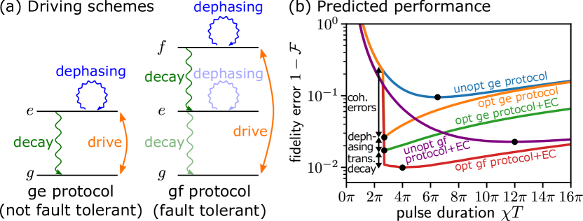
Figure 3: Combination of our optimization with the fault-tolerant scheme of [16, 17, 18]. (a) Comparison of the $ge$ driving scheme and the $gf$ driving scheme and their dominant transmon noise channels (dominant error channels have high saturation, second order processes have low saturation). (b) Theoretically predicted performance. The fidelity error is averaged over all possible target operations and the oscillations in $\chi T$ for different SNAP protocols (best performances highlighted by black dots, see Table S1 for a summary): unoptimized $ge$ protocol without error correction (EC) (blue), optimized $ge$ protocol without EC (orange), optimized $ge$ protocol with EC (green), unoptimized $gf$ protocol with EC (purple) and optimized $gf$ protocol with EC (red). The fidelity errors are estimated by perturbation theory (see Appendix F for more details).

While our approach focuses on the suppression of the coherent errors, the fault-tolerant scheme presented in [16, 17, 18] aims to reduce the incoherent errors from transmon decay and transmon dephasing. The key idea is to make the SNAP gate path-independent, i.e. that the final cavity-transmon state is independent of when, how many and which quantum jumps have occurred. This is achieved by including the second excited transmon state $f$ and making use of feedback.

In Fig. 3(b), we estimate theoretically how the fidelity error scales for different SNAP protocols for realistic parameter values. The SNAP gate is applied to the first four Fock modes. The error is averaged over all initial quantum states, all target operations, and over the oscillations in $\chi T$ (see Fig. 1(c)). As discussed above, the unoptimized $ge$ (blue) is operated best at intermediate gate times, while our scheme (orange) performs best at the optimization limit. The $ge$ SNAP protocol is in the limit of large gate times path-independent with respect to transmon decay errors [17]. By measuring the final transmon state transmon dephasing errors can be detected and corrected (green). Due to violations of the path-independence for finite gate times, a small error is remaining, which is discussed further in Section F.5. We obtain the best results by combining our approach with the $gf$ driving scheme (red), which is in the limit of large gate times path-independent with respect to transmon dephasing and decay [16, 17, 18]. The remaining errors are cavity decay (scaling with $T$) and the path-independence violations for transmon dephasing and decay for finite gate times.

In conclusion, our optimized SNAP gates completely suppress coherent errors, given that the gate time exceeds a certain threshold, and, in combination with the fault-tolerant scheme in [16, 17, 18], can further reduce incoherent errors. Furthermore, using our optimized SNAP gates together with displacement operations opens the way to efficiently implement arbitrary unitary operations [13, 14, 15]. While the optimization in this work was performed in simulations, we foresee the possibility of optimizing the pulse shapes directly based on experimental data, employing a feedback loop where pulse parameters are adapted suitably.

Competing interests

R.J.S. is a founder and shareholder of Quantum Circuits, Inc. The remaining authors declare no competing interests.

Appendix A Ideal SNAP gate dynamics for $T\gg 1/\chi$

With the system Hamiltonian (see Eq. 2) and an arbitrary drive function $\Omega(t)$, the Hamiltonian in the frame rotating with $\hat{H}_{0}+\hat{H}_{\chi}$ turns out to equal:

$$\hat{H}_{\mathrm{rot}}= \sum_{n}\left(\hat{\sigma}_{x}\real\left(\Omega(t)\mathrm{e}^{-\mathrm{i}\chi nt}\right)+\hat{\sigma}_{y}\imaginary\left(\Omega(t)\mathrm{e}^{-\mathrm{i}\chi nt}\right)\right)\outerproduct{n}{n}$$ (9)

with $\hat{\sigma}_{i}$ ($i=\{x,y,z\}$) as the Pauli operators. For the unoptimized drive (see Eq. 3) and performing a rotating wave approximation valid in the limit $T\gg 1/\chi$, the Hamiltonian simplifies to:

$$\hat{H}_{\mathrm{rot}}\approx\lambda\sum_{n}\hat{\sigma}_{\alpha_{n}}\outerproduct{n}{n}$$ (10)

with $\hat{\sigma}_{\alpha_{n}}=\hat{\sigma}_{x}\cos\alpha_{n}+\hat{\sigma}_{y}\sin\alpha_{n}$ as the $\hat{\sigma}_{x}$ Pauli operator rotated by the angle $\alpha_{n}$ around the positive $z$-axis. With the transmon intialized in the ground state $\ket{g}$ and the cavity in an arbitrary initial state $\sum_{n}c_{n}\ket{n}$, the time evolution of this state turns out to equal:

$$\ket{\psi(t)}=\sum_{n}c_{n}\left(\cos(\lambda t)\ket{gn}-\mathrm{i}\sin(\lambda t)\mathrm{e}^{\mathrm{i}\alpha_{n}}\ket{en}\right)$$ (11)

Setting the pulse amplitude to $\lambda=\pi/(2T)$, the target state of the first stage of the SNAP gate is reached:

$$\ket{\psi}_{\mathrm{target}}=\sum_{n}c_{n}\mathrm{e}^{\mathrm{i}\theta_{n}}\ket{en}$$ (12)

with the phase shifts $\theta_{n}=\alpha_{n}-\pi/2$.

Appendix B Graphical interpretation of the coherent errors

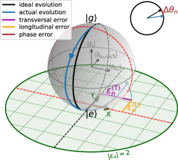
Figure S1: Geometrical definition of the coherent errors on the Bloch sphere. The final state of each Fock level dependent transmon state is projected onto the Lambert azimuthal equal-area projection plane (green). The elongation of the ideal trajectory in the projection plane ($Y$-direction, dashed black) determines the direction of the longitudinal error $\varepsilon_{n}^{(L)}$, its perpendicular line ($X$-direction, dashed red) the direction of the transversal error $\varepsilon_{n}^{(T)}$. The phase error $\Delta\theta_{n}$ is visualized in the phasor representation.

In this section, we show the connection between the quantum state error definition in Fast quantum control of cavities using an improved protocol without coherent errors and the geometrical interpretation, see Fig. 1(b). In the Bloch sphere coordinate system ($\langle\hat{\sigma}_{\alpha_{n}}\rangle$,$\langle\hat{\sigma}_{\alpha_{n}+\pi/2}\rangle$,$\langle\hat{\sigma}_{z}\rangle$), the ideal trajectory corresponds to a perfect half circle around the $(1,\ 0,\ 0)$ axis. The terminal state after the first stage of the SNAP gate (see Fast quantum control of cavities using an improved protocol without coherent errors) has the coordinates:

$$\begin{pmatrix}\langle\hat{\sigma}_{\alpha_{n}}\rangle\\ \langle\hat{\sigma}_{\alpha_{n}+\pi/2}\rangle\\ \langle\hat{\sigma}_{z}\rangle\end{pmatrix}=\begin{pmatrix}\sqrt{1-\frac{1}{4}\absolutevalue{\varepsilon_{n}}^{2}}\epsilon_{n}^{(T)}\\ \sqrt{1-\frac{1}{4}\absolutevalue{\varepsilon_{n}}^{2}}\epsilon_{n}^{(L)}\\ \frac{1}{2}\absolutevalue{\varepsilon_{n}}^{2}-1\end{pmatrix}$$ (13)

To identify a graphical interpretation, we use the Lambert azimuthal equal-area projection at the $\ket{e}$ point:

$$(X,\ Y)=\left(\sqrt{\frac{2}{1-\langle\hat{\sigma}_{z}\rangle}}\langle\hat{\sigma}_{\alpha_{n}}\rangle,\ \sqrt{\frac{2}{1-\langle\hat{\sigma}_{z}\rangle}}\langle\hat{\sigma}_{\alpha_{n}+\pi/2}\rangle\right)$$ (14)

The coordinates X and Y in the projection plane, turn out to equal $X=\epsilon_{n}^{(T)}$ and $Y=\epsilon_{n}^{(L)}$ for the terminal state. Thus, the transversal error corresponds to a deviation perpendicular to the ideal trajectory, while the longitudinal error corresponds to an over-/undershoot in direction of the ideal trajectory in the projection plane.

Appendix C Derivation of the optimization scheme

In this section, we investigate how our correction parameters of our optimized driving protocol (see Eq. 5) influence the coherent errors and can thus be used to correct these errors (see Eq. 6). Compared to the unoptimized driving scheme (see Eq. 3), our drive has three Fock-level-dependent correction parameters: the amplitude correction $\Delta\lambda_{n}=\lambda_{n}-\lambda$ with $\lambda=\pi/(2T)$, the frequency correction $\Delta\omega_{n}=\omega_{n}-\chi n$, and the phase correction $\Delta\alpha_{n}=\alpha_{n}-\theta_{n}-\pi/2$.

Amplitude correction We replace $\lambda$ in Eq. 11 by $\lambda_{n}=\pi/2T+\Delta\lambda_{n}$ and expand for small $\Delta\lambda_{n}$:

$$\ket{\psi(T)}\approx\sum_{n}c_{n}\left(-\Delta\lambda_{n}T\ket{gn}+\mathrm{e}^{\mathrm{i}\theta_{n}}\ket{en}\right)$$ (15)

Thus, amplitude corrections $\Delta\lambda_{n}$ create longitudinal errors $\varepsilon_{n}^{(L)}\approx\pi\Delta\lambda_{n}/\lambda$ on their associated Fock modes $n$, while the transversal and phase errors remain approximately zero.

Phase correction Substituting $\alpha_{n}$ in Eq. 11 by $\theta_{n}+\pi/2+\Delta\alpha_{n}$, the final state turns out to equal:

$$\ket{\psi(T)}=\sum_{n}c_{n}\mathrm{e}^{\mathrm{i}(\theta_{n}+\Delta\alpha_{n})}\ket{en}$$ (16)

Therefore, the amplitude shift $\Delta\alpha_{n}$ creates a phase error $\Delta\theta_{n}=\alpha_{n}$ and the other coherent errors remain zero.

Detuning The driving frequencies $\omega_{n}$ for each Fock mode $n$ are now detuned by $\Delta\omega_{n}$ from the unoptmized drive frequencies $\chi n$ with $\Delta\omega_{n}t\ll 1$:

$$\Omega(t) =\sum_{n}\lambda\mathrm{e}^{\mathrm{i}(\chi nt+\Delta\omega_{n}t+\alpha_{n})}\overset{\Delta\omega_{n}t\ll 1}{\approx}\sum_{n}\lambda\left(1+\mathrm{i}\Delta\omega_{n}t\right)\mathrm{e}^{\mathrm{i}(\chi nt+\alpha_{n})}$$ (17)

By inserting this pulse into Eq. 9 and taking only terms close to resonance into account, our Hamiltonian reads as:

$$\hat{H}_{\mathrm{rot}}\approx\sum_{n}\left(\lambda\hat{\sigma}_{\alpha_{n}}+\lambda\Delta\omega_{n}t\hat{\sigma}_{\alpha_{n}+\pi/2}\right)\outerproduct{n}{n}$$ (18)

The first summand in this Hamiltonian corresponds to the ideal dynamics (see also Appendix A), the second term results from the detuning.

We now switch into the frame moving along with the ideal trajectory:

$$\begin{split}\hat{\widetilde{H}}_{\mathrm{rot}}\approx\sum_{n}\lambda\Delta\omega_{n}t&\left(\hat{\sigma}_{\alpha_{n}+\pi/2}\cos(2\lambda t)-\hat{\sigma}_{z}\sin(2\lambda t)\right)\outerproduct{n}{n}\end{split}$$ (19)

which leads us to the time evolution operator in this frame:

$$\hat{\widetilde{U}} \approx\hat{\mathds{1}}-i\int_{0}^{T}\hat{\widetilde{H}}_{\mathrm{rot}}(t)\,dt=\hat{\mathds{1}}+\sum_{n}\mathrm{i}\Delta\omega_{n}T\left(\frac{1}{\pi}\hat{\sigma}_{\alpha_{n}+\pi/2}+\frac{1}{2}\hat{\sigma}_{z}\right)\outerproduct{n}{n}$$ (20)

Thus, the final state back in the original frame turns out to equal:

$$\ket{\psi(T)}\approx\sum_{n}c_{n}\left(\frac{\mathrm{i}}{\pi}\Delta\omega_{n}T\ket{gn}+\mathrm{e}^{\mathrm{i}(\theta_{n}+\Delta\omega_{n}T/2)}\ket{en}\right)$$ (21)

with a vanishing longitudinal error, a transversal error $\varepsilon_{n}^{(T)}\approx-\Delta\omega_{n}/\lambda$ and a phase error $\theta_{n}\approx\Delta\omega_{n}T/2$. To compensate for the unwanted phase shift, the drive phases are modified in Eq. 5 by $-\Delta\omega_{n}T/2$ and thus we can freely control the transversal error without disturbing the phase.

As demonstrated, each of the coherent errors can be individually controlled by one of the correction parameters of our optimized pulse shape. Even though our derivation is performed in the limit of large pulse durations $T$ and small correction parameters, iteratively reapplying Eq. 6 leads to optimized pulse sequences far beyond the validity range of our approximations.

Appendix D Kerr nonlinearity and correction to the dispersive coupling

For the application in the actual experiment also higher order contributions to the Hamiltonian in Eq. 2 have to be considered. This includes the Kerr nonlinearity $\hat{H}_{\mathrm{Kerr}}=-(K/2)\hat{a}^{{\dagger}^{2}}\hat{a}^{2}$ and the correction to the dispersive coupling $\hat{H}_{\chi^{\prime}}=(\chi^{\prime}/2)\outerproduct{e}{e}\hat{a}^{{\dagger}^{2}}\hat{a}^{2}$. To understand their effect on the dynamics of the SNAP gate, we transform the Hamiltonian into the frame rotating with $\hat{H}_{0}+\hat{H}_{\chi}+\hat{H}_{\mathrm{Kerr}}+\hat{H}_{\chi^{\prime}}$:

$$\begin{split}\hat{H}_{\mathrm{rot}}&=\sum_{n}\left[\hat{\sigma}_{x}\real\left(\Omega(t)\mathrm{e}^{-\mathrm{i}\left(\chi n-\frac{1}{2}\chi^{\prime}(n^{2}-n)\right)t}\right)+\hat{\sigma}_{y}\imaginary\left(\Omega(t)\mathrm{e}^{-\mathrm{i}\left(\chi n-\frac{1}{2}\chi^{\prime}(n^{2}-n)\right)t}\right)\right]\outerproduct{n}{n}\end{split}$$ (22)

So, to drive the $\ket{gn}\leftrightarrow\ket{en}$ resonantly, we replace the driving frequencies by $\omega_{n}=\chi n-\chi^{\prime}(n^{2}-n)/2$. Using the rotating wave approximation, the Hamiltonian is again identical with Eq. 10. However, the target operation is defined in the system rotating with $\hat{H}_{0}+\hat{H}_{\chi}$. This change in frame has to be compensated by setting the unoptimized drive phases $\alpha_{n}$ to $\theta_{n}+\pi/2-(K-\chi^{\prime})(n^{2}-n)T/2$. In the limit of large pulse durations, and neglecting noise, this implements again the first stage of the SNAP gate.

Appendix E Full system dynamics including the second excited transmon state and noise

E.1 System Hamiltonian including the second excited transmon state

Including the second excited transmon state $\ket{f}$, we redefine the components of our system Hamiltonian $\hat{H}=\hat{H}_{0}+\hat{H}_{\chi}+\hat{H}_{\mathrm{drive}}$ as:

$$\hat{H}_{0} =\omega_{ge}\outerproduct{e}{e}+\omega_{gf}\outerproduct{f}{f}$$ (23a)

$$\hat{H}_{\chi} =-\chi\outerproduct{e}{e}\hat{a}^{\dagger}\hat{a}-\chi_{f}\outerproduct{f}{f}\hat{a}^{\dagger}\hat{a}$$ (23b)

with $\omega_{gf}$ as the transition frequency between the ground and second excited transmon state $\ket{g}$ and $\ket{f}$, and $\chi_{f}$ as the dispersive coupling frequency with the $\ket{f}$ state. To make the gf SNAP protocol fault-tolerant with respect to transmon decay, we set $\chi_{f}=\chi$ to fulfill the $\chi$-matching condition [16, 17, 18] in our analysis. For the ge drive protocol, the drive Hamiltonian $\hat{H}_{\mathrm{drive}}$ is defined in the main text, for the gf protocol by $\hat{H}_{\mathrm{drive}}=\Omega(t)\mathrm{e}^{-\mathrm{i}\omega_{gf}t}\outerproduct{f}{g}+\mathrm{H.c.}$. For simplicity, we neglect the Kerr nonlinearity and the correction to the dispersive coupling in the comparison between the different driving protocols.

In the frame comoving with $\hat{H}_{0}+\hat{H}_{\chi}$, the Hamiltonian for the gf SNAP protocol equals:

$$\hat{H}_{\mathrm{rot}}=\sum_{n}\left((\outerproduct{f}{g}+\outerproduct{g}{f})\real\left(\Omega(t)\mathrm{e}^{-\mathrm{i}\chi nt}\right)+\mathrm{i}(\outerproduct{f}{g}-\outerproduct{g}{f})\imaginary\left(\Omega(t)\mathrm{e}^{-\mathrm{i}\chi nt}\right)\right)\otimes\outerproduct{n}{n}$$ (24)

Using the rotating wave approximation and the unoptimized drive (see Eq. 3), this simplifies to:

$$\hat{H}_{\mathrm{rot}}\approx\lambda\sum_{n}\left(\exp(\mathrm{i}\alpha_{n})\outerproduct{f}{g}+\exp(-\mathrm{i}\alpha_{n})\outerproduct{g}{f}\right)\otimes\outerproduct{n}{n}$$ (25)

Therefore, the time evolution for an initial state $\ket{\psi(0)}=\sum_{n}c_{n}\ket{gn}$ turns out to equal (compare to Eq. 11):

$$\ket{\psi(t)}=\sum_{n}c_{n}\left(\cos(\lambda t)\ket{gn}-\mathrm{i}\sin(\lambda t)\mathrm{e}^{\mathrm{i}\alpha_{n}}\ket{fn}\right)$$ (26)

For $\lambda=\pi/(2T)$, the target state of the first stage of the SNAP gate is reached:

$$\ket{\psi}_{\mathrm{target}}=\sum_{n}c_{n}\mathrm{e}^{\mathrm{i}\theta_{n}}\ket{fn}$$ (27)

E.2 Non-unitary time evolution

Above, we developed a scheme to completely suppress the coherent errors. We considered noise only indirectly as we also minimized the gate time. However, to maximize the gate performance we have to optimize the total error including noise. The dominant noise channels are transmon decay, transmon dephasing and cavity decay. The corresponding Lindblad operators in the frame comoving with $\hat{H}_{0}+\hat{H}_{\chi}$ are given by [18]:

$$\hat{L}_{e\rightarrow g} =\mathrm{e}^{\mathrm{i}\chi\hat{a}^{\dagger}\hat{a}t}\outerproduct{g}{e}$$ (28a)

$$\hat{L}_{f\rightarrow e} =\mathrm{e}^{\mathrm{i}(\chi_{f}-\chi)\hat{a}^{\dagger}\hat{a}t}\outerproduct{e}{f}$$ (28b)

$$\hat{L}_{ee} =\outerproduct{e}{e}$$ (28c)

$$\hat{L}_{ff} =\outerproduct{f}{f}$$ (28d)

$$\hat{L}_{\mathrm{cav}} =\mathrm{e}^{\mathrm{i}(\chi\outerproduct{e}{e}+\chi_{f}\outerproduct{f}{f})t}\hat{a}$$ (28e)

with $L_{e\rightarrow g}$ and $L_{f\rightarrow e}$ as the transmon decay operators, $L_{ee}$ and $L_{ff}$ as the transmon dephasing operators, and $L_{\mathrm{cav}}$ as the cavity decay operator.

The time evolution of the density matrix $\hat{\rho}$ under the influence of noise is described by the Lindblad Master equation:

$$\frac{\mathrm{d}\hat{\rho}}{\mathrm{d}t}=-\mathrm{i}\left[\hat{H}_{\mathrm{rot}},\hat{\rho}\right]+\sum_{j}\Gamma_{j}\left(\hat{L}_{j}\hat{\rho}\hat{L}_{j}^{\dagger}-\frac{1}{2}\left\{\hat{\rho},\hat{L}_{j}^{\dagger}\hat{L}_{j}\right\}\right)$$ (29)

with $\hat{H}_{\mathrm{rot}}$ as the Hamiltonian in the rotating frame comoving with $\hat{H}_{0}+\hat{H}_{\chi}$. The sum iterates over all noise contributions with $\Gamma_{j}$ as the corresponding noise rate.

E.3 Propagation of errors during the ge SNAP gate and definition of the mean squared overlap

Here, we analyze following [18], how transmon decay and dephasing errors are propagated during the ge SNAP gate operation in the limit of large $\chi T$, where the system Hamiltonian is given by Eq. 10. Initially, the system is in the state $\ket{\psi_{\mathrm{in}}}=\sum_{n}c_{n}\ket{gn}$. The time evolution consists of three steps: First, the the dynamics follow the idealized system Hamiltonian from Eq. 10 up to the time $t=t_{j}$, where a quantum jump event (either transmon decay or dephasing) occurs. After the jump, the evolution follows again the idealized Hamiltonian up to $t=T$.

For a single transmon dephasing event at $t_{j}$, the final quantum state turns out to equal:

$$\ket{\psi(T)} \propto\mathrm{e}^{-\mathrm{i}\hat{H}_{\mathrm{rot}}(T-t_{j})}\hat{L}_{ee}\mathrm{e}^{-\mathrm{i}\hat{H}_{\mathrm{rot}}t_{j}}\ket{\psi_{\mathrm{in}}}$$ (30a)

$$\propto-\sin(\lambda(T-t_{j}))\ket{\psi_{\mathrm{in}}}+\cos(\lambda(T-t_{j}))\ket{\psi_{\mathrm{target}}}$$ (30b)

Directly after the first stage of the SNAP gate was performed, we measure the qubit state. If the outcome is $\ket{e}$, the final state equals the target state $\ket{\psi_{\mathrm{target}}}=\sum_{n}c_{n}\mathrm{e}^{\mathrm{i}\theta_{n}}\ket{en}$. If we measure $\ket{g}$, the state is the initial state $\ket{\psi_{\mathrm{in}}}$, as if no pulse would have been applied. To correct this error, one has to reapply the SNAP pulse. These results are independent of the actual jump time and so the $ge$ SNAP protocol is fault tolerant for at least one dephasing event. Based on this result, we define the target states for a measurement outcome $\ket{g}$ and $\ket{e}$ as:

$$\ket{\psi_{\mathrm{target},g}} =\ket{\psi_{\mathrm{in}}}=\sum_{n}c_{n}\ket{gn}$$ (31a)

$$\ket{\psi_{\mathrm{target},e}} =\ket{\psi_{\mathrm{target}}}=\sum_{n}c_{n}\mathrm{e}^{\mathrm{i}\theta_{n}}\ket{en}$$ (31b)

Repeating the same analysis for transmon decay $e\rightarrow g$, results in:

$$\ket{\psi(T)} \propto\mathrm{e}^{-\mathrm{i}\hat{H}_{\mathrm{rot}}(T-t_{j})}\hat{L}_{e\rightarrow g}\mathrm{e}^{-\mathrm{i}\hat{H}_{\mathrm{rot}}t_{j}}\ket{\psi(0)}$$ (32a)

$$\propto\sum_{n\in\mathcal{N}}c_{n}\mathrm{e}^{\mathrm{i}(\chi nt_{j}+\theta_{n})}\left[\cos(\lambda(T-t_{j}))\ket{gn}+\sin(\lambda(T-t_{j}))\mathrm{e}^{\mathrm{i}\theta_{n}}\ket{en}\right]$$ (32b)

As the final state after an $\ket{g}$ and $\ket{e}$ measurement depends on the jump time $t_{j}$, the ge SNAP protocol is not fault tolerant with respect to transmon decay.

Based on the target states in Eq. 31, we define the the mean squared overlap for ge protocol without error correction as (see Eq. 7):

$$\mathcal{F}=\underset{\begin{subarray}{c}\vec{c}\text{ s.t.}\\ \norm{c}=1\end{subarray}}{\mathrm{avg}}\bra{\psi_{\mathrm{target},e}(\vec{c})}\hat{\rho}_{\mathrm{out}}(\vec{c})\ket{\psi_{\mathrm{target},e}(\vec{c})}$$ (33)

and for the ge protocol with error correction:

$$\mathcal{F}=\underset{\begin{subarray}{c}\vec{c}\text{ s.t.}\\ \norm{c}=1\end{subarray}}{\mathrm{avg}}\sum_{j=\{g,e\}}\bra{\psi_{\mathrm{target},j}(\vec{c})}\hat{\rho}_{\mathrm{out}}(\vec{c})\ket{\psi_{\mathrm{target},j}(\vec{c})}$$ (34)

with $\hat{\rho}_{\mathrm{out}}(\vec{c})$ as the density matrix of the cavity-transmon system after the first stage of the SNAP gate.

E.4 Propagation of errors during the gf SNAP gate and definition of the mean squared overlap

In this section, we repeat the procedure of Section E.3 for the gf SNAP protocol in the limit of large gate times, where the Hamiltonian is approximated by Eq. 25. The two dominant noise channels are $f\rightarrow e$ decay and transmon dephasing. As the ideal SNAP evolution now ends in the $f$ state, we redefine the target state as $\ket{\psi_{\mathrm{target}}}=\sum_{n}c_{n}\mathrm{e}^{\mathrm{i}\theta_{n}}\ket{fn}$. If a dephasing event occurs at time $t=t_{j}$, the final system state is given by:

$$\ket{\psi(T)} \propto\mathrm{e}^{-\mathrm{i}\hat{H}_{\mathrm{rot}}(T-t_{j})}\hat{L}_{ff}\mathrm{e}^{-\mathrm{i}\hat{H}_{\mathrm{rot}}t_{j}}\ket{\psi_{\mathrm{in}}}$$ (35a)

$$\propto-\sin(\lambda(T-t_{j}))\ket{\psi_{\mathrm{in}}}+\cos(\lambda(T-t_{j}))\ket{\psi_{\mathrm{target}}}$$ (35b)

In case of an $f\rightarrow e$ decay event, the final state is:

$$\ket{\psi(T)} \propto\mathrm{e}^{-\mathrm{i}\hat{H}_{\mathrm{rot}}(T-t_{j})}\hat{L}_{f\rightarrow e}\mathrm{e}^{-\mathrm{i}\hat{H}_{\mathrm{rot}}t_{j}}\ket{\psi_{\mathrm{in}}}$$ (36a)

$$\propto\sum_{n\in\mathcal{N}}c_{n}\mathrm{e}^{\mathrm{i}\left((\chi_{f}-\chi)nt_{j}+\theta_{n}\right)}\ket{en}\overset{\chi=\chi_{f}}{=}\sum_{n}c_{n}\mathrm{e}^{\mathrm{i}\theta_{n}}\ket{en}$$ (36b)

Thus, the measurement result $\ket{g}$ corresponds to a dephasing error and the system ends up in its initial state. The measurement result $\ket{e}$ corresponds to a transmon decay error, where the cavity state was correctly prepared, but the transmon ends up in $\ket{e}$. This can be corrected by simply flipping the transmon state. In case of an $\ket{f}$ measurement, the SNAP gate was successfully applied. Correspondingly, we define the target states for the different measurement outcomes as:

$$\ket{\psi_{\mathrm{target},g}} =\ket{\psi_{\mathrm{in}}}=\sum_{n}c_{n}\ket{gn}$$ (37a)

$$\ket{\psi_{\mathrm{target},e}} =\sum_{n}c_{n}\mathrm{e}^{\mathrm{i}\theta_{n}}\ket{en}$$ (37b)

$$\ket{\psi_{\mathrm{target},f}} =\ket{\psi_{\mathrm{target}}}=\sum_{n}c_{n}\mathrm{e}^{\mathrm{i}\theta_{n}}\ket{fn}$$ (37c)

Therefore, we define the mean squared overlap for the gf SNAP gate with error correction as:

$$\mathcal{F}=\underset{\begin{subarray}{c}\vec{c}\text{ s.t.}\\ \norm{c}=1\end{subarray}}{\mathrm{avg}}\sum_{j=\{g,e,f\}}\bra{\psi_{\mathrm{target},j}(\vec{c})}\hat{\rho}_{\mathrm{out}}(\vec{c})\ket{\psi_{\mathrm{target},j}(\vec{c})}$$ (38)

Appendix F Estimation of the dominant error contributions

In the following sections, we derive analytically the dominant error contributions for the various SNAP gate implementations mentioned in the main text. The dominant errors include the coherent errors, transmon decay, transmon dephasing, cavity decay and path-independence violations. The errors are always averaged over all initial cavity states, defined by the amplitude vector $\vec{c}$, all possible target operations, given by $\vec{\theta}$, and the oscillations in $\chi T$.

F.1 Coherent errors

Here, we derive the coherent error contributions in the limit of large $\chi T$ for the unoptimized pulse from Eq. 3 and the scaling law of the mean-squared-overlap error. The notation throughout this section is for the $ge$ SNAP protocol, but the result is the same for the $gf$ protocol.

Using the unoptimized drive (see Eq. 3), we rewrite the Hamiltonian from Eq. 9 as:

$$\hat{H}_{\mathrm{rot}}=\sum_{n}\sum_{m}\lambda\hat{\sigma}_{(\chi T(m-n)+\alpha_{m})}\outerproduct{n}{n}$$ (39)

with $\hat{\sigma}_{\alpha}=\hat{\sigma}_{x}\cos\alpha+\hat{\sigma}_{y}\sin\alpha$ as a Pauli operator rotated by $\alpha$ around the z axis. We transform this Hamiltonian into the frame rotating with the idealized SNAP Hamiltonian from Eq. 10:

$$\begin{split}\hat{\widetilde{H}}_{\mathrm{rot}}&=\sum_{n}\sum_{m\neq n}\lambda\left[\cos^{2}(\lambda t)\hat{\sigma}_{(\chi t(m-n)+\alpha_{m})}+\sin^{2}(\lambda t)\hat{\sigma}_{(2\alpha_{n}-\alpha_{m}-\chi t(m-n))}+\right.\\ &\qquad\qquad\left.+\sin(2\lambda t)\sin(\alpha_{n}-\alpha_{m}-\chi t(m-n))\hat{\sigma}_{z}\right]\outerproduct{n}{n}\end{split}$$ (40)

The time evolution operator in this rotating frame is given by:

$$\hat{\widetilde{U}} =\hat{\mathds{1}}-\mathrm{i}\int_{0}^{T}\,dt\,\hat{\widetilde{H}}_{\mathrm{rot}}(t)-\int_{0}^{T}\,dt\int_{0}^{t}\,dt^{\prime}\hat{\widetilde{H}}_{\mathrm{rot}}(t)\hat{\widetilde{H}}_{\mathrm{rot}}(t^{\prime})+\mathrm{...}$$ (41)

Solving the integrals, sorting in powers of $1/(\chi T)$ and applying the time evolution operator to the initial state $\ket{gn}$, results in:

$$\hat{\widetilde{U}}\ket{gn}=\ket{gn}+\sum_{m\neq n}\frac{\pi}{2(m-n)\chi T}\left[\mathrm{e}^{\mathrm{i}((n-m)\chi T+2\alpha_{n}-\alpha_{m})}+\mathrm{e}^{\mathrm{i}\alpha_{m}}-\mathrm{e}^{\mathrm{i}\alpha_{n}}\right]\ket{en}+\mathcal{O}((\chi T)^{-2})$$ (42)

By transforming the result back into the frame rotating with $\hat{H}_{0}+\hat{H}_{\chi}$, we receive the final state $|\psi_{\mathrm{out}}\rangle$:

$$|\psi_{\mathrm{out}}\rangle=\sum_{n}\Big{(}\mathrm{e}^{\mathrm{i}\theta_{n}}\ket{en}+\sum_{m\neq n}\frac{-\mathrm{i}\pi}{2(m-n)\chi T}\big{(}\mathrm{e}^{\mathrm{i}((n-m)\chi T+\theta_{n}-\theta_{m})}+\mathrm{e}^{\mathrm{i}(\theta_{m}-\theta_{n})}-1\big{)}\ket{gn}\Big{)}+\mathcal{O}((\chi T)^{-2})$$ (43)

with the coherent error contributions (see Fast quantum control of cavities using an improved protocol without coherent errors):

$$\varepsilon_{n} =\sum_{m\neq n}\frac{\mathrm{i}\pi}{(m-n)\chi T}\left[\mathrm{e}^{\mathrm{i}((n-m)\chi T+\theta_{n}-\theta_{m})}+\mathrm{e}^{\mathrm{i}(\theta_{m}-\theta_{n})}-1\right]+\mathcal{O}((\chi T)^{-2})$$ (44a)

$$\Delta\theta_{n} =\mathcal{O}((\chi T)^{-2})$$ (44b)

$\varepsilon_{n}$, and so also the longitudinal and transversal errors, scale with $1/(\chi T)$. Our calculations show that the phase error $\Delta\theta_{n}$ scales at least with $1/(\chi T)^{2}$. Our simulations confirm that $1/(\chi T)^{2}$ is the correct scaling law.

The mean squared overlaps $\mathcal{F}_{g}$ and $\mathcal{F}_{e}$ with the target states $\ket{\psi_{\mathrm{target},g}}$ and $\ket{\psi_{\mathrm{target},e}}$ turn out to equal:

$$\mathcal{F}_{g} =\underset{\begin{subarray}{c}\vec{c}\in\mathbb{C}^{L}\text{ s.t.}\\ \norm{c}=1\end{subarray}}{\mathrm{avg}}\absolutevalue{\langle\psi_{\mathrm{target},g}|\psi_{\mathrm{out}}\rangle}^{2}=\underset{\begin{subarray}{c}\vec{c}\in\mathbb{C}^{L}\text{ s.t.}\\ \norm{c}=1\end{subarray}}{\mathrm{avg}}\frac{1}{4}\absolutevalue{\sum_{n}\absolutevalue{c_{n}}^{2}\epsilon_{n}}^{2}=\frac{1}{4}\sum_{n,n^{\prime}}\overbrace{\underset{\begin{subarray}{c}\vec{c}\in\mathbb{C}^{L}\text{ s.t.}\\ \norm{c}=1\end{subarray}}{\mathrm{avg}}(\absolutevalue{c_{n}c_{n^{\prime}}}^{2})}^{=(1+\delta_{n,n^{\prime}})/(L(L+1))}\epsilon_{n^{\prime}}^{\ast}\epsilon_{n}=\sum_{n,n^{\prime}}\frac{1+\delta_{n,n^{\prime}}}{4L(L+1)}\epsilon_{n^{\prime}}^{\ast}\epsilon_{n}$$ (45)

$$\mathcal{F}_{e} =\underset{\begin{subarray}{c}\vec{c}\in\mathbb{C}^{L}\text{ s.t.}\\ \norm{c}=1\end{subarray}}{\mathrm{avg}}\absolutevalue{\langle\psi_{\mathrm{target},e}|\psi_{\mathrm{out}}\rangle}^{2}=\underset{\begin{subarray}{c}\vec{c}\in\mathbb{C}^{L}\text{ s.t.}\\ \norm{c}=1\end{subarray}}{\mathrm{avg}}\absolutevalue{\sum_{n}\absolutevalue{c_{n}}^{2}\sqrt{1-\absolutevalue{\epsilon_{n}}^{2}}\mathrm{e}^{\mathrm{i}\Delta\theta_{n}}}^{2}$$ (46a)

$$=\sum_{n,n^{\prime}}\overbrace{\underset{\begin{subarray}{c}\vec{c}\in\mathbb{C}^{L}\text{ s.t.}\\ \norm{c}=1\end{subarray}}{\mathrm{avg}}(\absolutevalue{c_{n}c_{n^{\prime}}}^{2})}^{=(1+\delta_{n,n^{\prime}})/(L(L+1))}\left[\sqrt{(1-\absolutevalue{\varepsilon_{n}}^{2}/4)(1-\absolutevalue{\varepsilon_{n^{\prime}}}^{2}/4)}\mathrm{e}^{\mathrm{i}(\Delta\theta_{n}-\Delta\theta_{n^{\prime}})}\right]=$$ (46b)

$$=1-\frac{1}{L}\sum_{n}\frac{\absolutevalue{\epsilon_{n}}^{2}}{4}+\mathcal{O}((\chi T)^{-3})$$ (46c)

with $L$ as the number of Fock modes part of the target operation.

Next, we derive the squared mean overlap error averaged over the target phases and $\chi T$ oscillations. Using Eq. 44, we get the relation:

$$\underset{\vec{\theta},\ \chi T\mathrm{osc.}}{\mathrm{avg}}\varepsilon_{n^{\prime}}^{\ast}\varepsilon_{n}=\left(\frac{\pi}{\chi T}\right)^{2}\sum_{\begin{subarray}{c}m,m^{\prime}\\ m\neq n\\ m^{\prime}\neq n^{\prime}\end{subarray}}\frac{1}{(m-n)(m^{\prime}-n^{\prime})}\left[2\delta_{n,n^{\prime}}\delta_{m,m^{\prime}}+1\right]+\mathcal{O}((\chi T)^{-3})$$ (47)

Thus, the averaged mean squared overlaps equal:

$$\underset{\vec{\theta},\ \chi T\mathrm{osc.}}{\mathrm{avg}}\mathcal{F}_{g}=\frac{5}{4L(L+1)}\left(\frac{\pi}{\chi T}\right)^{2}\sum_{\begin{subarray}{c}n,m\\ m\neq n\end{subarray}}\frac{1}{(m-n)^{2}}+\mathcal{O}((\chi T)^{-3})$$ (48)

$$\underset{\vec{\theta},\ \chi T\mathrm{osc.}}{\mathrm{avg}}\mathcal{F}_{e}=1-\frac{3}{4L}\left(\frac{\pi}{\chi T}\right)^{2}\sum_{\begin{subarray}{c}n,m\\ m\neq n\end{subarray}}\frac{1}{(m-n)^{2}}+\mathcal{O}((\chi T)^{-3})$$ (49)

For all unoptimized SNAP protocols in Fig. 3 without error correction, the coherent error contribution is estimated by $1-\underset{\vec{\theta},\ \chi T\mathrm{osc.}}{\mathrm{avg}}\mathcal{F}_{e}$, for all unoptmized protocols with error correction, by $1-\underset{\vec{\theta},\ \chi T\mathrm{osc.}}{\mathrm{avg}}\mathcal{F}_{g}-\underset{\vec{\theta},\ \chi T\mathrm{osc.}}{\mathrm{avg}}\mathcal{F}_{e}$.

F.2 $e\rightarrow g$ decay

In this section, we derive the transmon decay error for the $ge$ SNAP gate in the limit of $\chi T\to\infty$, but $\Gamma_{e\rightarrow g}T\to 0$. All other noise rates are set to zero throughout this section. We first expand the density matrix in orders of $\Gamma_{e\rightarrow g}T$:

$$\hat{\rho}(t)=\hat{\rho}_{0}(t)+\hat{\rho}_{1}(t)+...$$ (50)

where $\hat{\rho}_{j}(t)$ is of order $(\Gamma_{e\rightarrow g}T)^{j}$. With this expansion of the density matrix and the idealized Hamiltonian from Eq. 10, we sort the Lindblad Master equation from Eq. 29 in orders of $\Gamma_{e\rightarrow g}T$:

$$\derivative{\hat{\rho}_{0}(t)}{t} =-\mathrm{i}[\lambda\sum_{n}\hat{\sigma}_{\alpha_{n}}\outerproduct{n}{n},\hat{\rho}_{0}(t)]$$ (51a)

$$\derivative{\hat{\rho}_{1}(t)}{t} =-\mathrm{i}[\lambda\sum_{n}\hat{\sigma}_{\alpha_{n}}\outerproduct{n}{n},\hat{\rho}_{1}(t)]+\Gamma_{e\rightarrow g}\left[\hat{L}_{e\rightarrow g}\hat{\rho}_{0}(t)\hat{L}^{\dagger}_{e\rightarrow g}-\frac{1}{2}\left\{\hat{\rho}_{0}(t),\hat{L}^{\dagger}_{e\rightarrow g}\hat{L}_{e\rightarrow g}\right\}\right]$$ (51b)

$$\mathmakebox[\widthof{{}={}}][c]{\vdots}$$ (51c)

The solution for the unperturbed density matrix $\hat{\rho}_{0}$ is simply given by the coherent evolution:

$$\hat{\rho}_{0}(t)=\outerproduct{\psi(t)}{\psi(t)}$$ (52)

with the idealized time evolution of the quantum state $\ket{\psi(t)}$, defined in Eq. 11. To solve Eq. 51b, we go into the frame comoving with the ideal trajectory. With the ideal time evolution operator $\hat{U}(t)=\mathrm{exp}\left(-\mathrm{i}\sum_{n}\lambda\hat{\sigma}_{\alpha_{n}}\outerproduct{n}{n}t\right)$ and $\hat{\widetilde{\rho}}_{1}(t)=\hat{U}(t)^{\dagger}\hat{\rho}_{1}(t)\hat{U}(t)$, Eq. 51b can be rewritten as:

$$\derivative{\hat{\widetilde{\rho}}_{1}(t)}{t} =\Gamma_{e\rightarrow g}\hat{U}(t)^{\dagger}\left[\hat{L}_{e\rightarrow g}\hat{\rho}_{0}(t)\hat{L}^{\dagger}_{e\rightarrow g}-\frac{1}{2}\left\{\hat{\rho}_{0}(t),\hat{L}^{\dagger}_{e\rightarrow g}\hat{L}_{e\rightarrow g}\right\}\right]\hat{U}(t)$$ (53a)

$$\begin{split}&=\Gamma_{e\rightarrow g}\big{[}\sum_{n,n^{\prime}}c_{n}c_{n^{\prime}}^{\ast}\overbrace{\mathrm{e}^{\mathrm{i}\chi(n-n^{\prime})t}}^{\xrightarrow[]{\begin{subarray}{c}\text{rotating}\\ \text{wave approx.}\end{subarray}}\delta_{n,n^{\prime}}}\mathrm{e}^{\mathrm{i}(\theta_{n}-\theta_{n^{\prime}})}\sin^{2}(\lambda t)\hat{U}^{\dagger}(t)|gn\rangle\langle gn^{\prime}|\hat{U}(t)\\ &\quad-\frac{1}{2}\hat{U}^{\dagger}(t)\left\{\outerproduct{\psi(t)}{\psi(t)},\outerproduct{e}{e}\right\}\hat{U}(t)\big{]}\end{split}$$ (53b)

Using the rotating wave approximation, we ignore all fast oscillating terms. With $\hat{\widetilde{\rho}}_{1}(0)=0$, $\hat{\widetilde{\rho}}_{1}(T)$ is obtained by integrating LABEL:equ:eg_decay_step in time. Transforming the result back into the original frame, we receive:

$$\begin{split}\hat{\rho}_{1}(T)=\Gamma_{e\rightarrow g}T\left[\sum_{n}\absolutevalue{c_{n}}^{2}\begin{pmatrix}\frac{3}{8}&\frac{1}{2\pi}\mathrm{e}^{-\mathrm{i}\theta_{n}}\\ \frac{1}{2\pi}\mathrm{e}^{\mathrm{i}\theta_{n}}&\frac{1}{8}\end{pmatrix}\otimes\outerproduct{n}{n}\right.\left.-\frac{1}{2}\sum_{n,n^{\prime}}c_{n}c_{n^{\prime}}^{\ast}\begin{pmatrix}0&-\frac{1}{\pi}\mathrm{e}^{-\mathrm{i}\theta_{n^{\prime}}}\\ -\frac{1}{\pi}\mathrm{e}^{\mathrm{i}\theta_{n}}&\mathrm{e}^{\mathrm{i}(\theta_{n}-\theta_{n^{\prime}})}\end{pmatrix}\otimes\outerproduct{n}{n^{\prime}}\right]\end{split}$$ (54)

Thus, we get the mean squared overlaps:

$$\mathcal{F}_{g}=\frac{3}{4(L+1)}\Gamma_{e\rightarrow g}T+\mathcal{O}((\Gamma_{e\rightarrow g}T)^{2},(\Gamma_{e\rightarrow g}T)(\chi T)^{-1})$$ (55)

$$\mathcal{F}_{e}=1-\frac{2L+1}{4(L+1)}\Gamma_{e\rightarrow g}T+\mathcal{O}((\Gamma_{e\rightarrow g}T)^{2},(\Gamma_{e\rightarrow g}T)(\chi T)^{-1})$$ (56)

The ge SNAP protocol without error correction has an error contribution of $1-\mathcal{F}_{e}$, the ge SNAP protocol with error correction has an error of $1-\mathcal{F}_{g}-\mathcal{F}_{e}$. In contrast, the gf SNAP protocol with error correction is fault tolerant with respect to the dominant transmon decay channel, namely the $f\rightarrow e$ decay, in the limit of large $\chi T$. Therefore, it does not suffer from transmon decay in first order. However, for finite $\chi T$ the path-independence is violated. The resulting errors are further discussed in Section F.5.

F.3 Transmon dephasing

In analogy to Section F.2, we derive in this section the effect of transmon dephasing on the ge SNAP protocol in the limit of $\chi T\to\infty$ and $\Gamma_{ee}T\to 0$. Expanding the density matrix $\hat{\rho}(t)=\hat{\rho}_{0}(t)+\hat{\rho}_{1}(t)+...$ in orders of $\Gamma_{ee}T$ and ordering the Lindblad Master equation in orders of $\Gamma_{ee}T$, results in:

$$\derivative{\hat{\rho}_{0}(t)}{t} =-\mathrm{i}[\lambda\sum_{n}\hat{\sigma}_{\alpha_{n}}\outerproduct{n}{n},\hat{\rho}_{0}(t)]$$ (57a)

$$\derivative{\hat{\rho}_{1}(t)}{t} =-\mathrm{i}[\lambda\sum_{n}\hat{\sigma}_{\alpha_{n}}\outerproduct{n}{n},\hat{\rho}_{1}(t)]+\Gamma_{ee}\left[\hat{L}_{ee}\hat{\rho}_{0}(t)\hat{L}^{\dagger}_{ee}-\frac{1}{2}\left\{\hat{\rho}_{0}(t),\hat{L}^{\dagger}_{ee}\hat{L}_{ee}\right\}\right]$$ (57b)

$$\mathmakebox[\widthof{{}={}}][c]{\vdots}$$ (57c)

with $\hat{L}_{ee}$ as the Lindblad operator for dephasing, see Eq. 28c. The solution for the unperturbed density matrix $\hat{\rho}_{0}$ is given by Eq. 52. As in Section F.2, we solve Eq. 57b by transforming it into the frame comoving with the ideal trajectory and integrate it in time, with $\hat{\rho}_{1}(0)=0$. The final state $\hat{\rho}_{1}(T)$ turns out to equal:

$$\hat{\rho}_{1}(T)=\frac{1}{8}\Gamma_{ee}T\sum_{n,n^{\prime}}c_{n}c_{n^{\prime}}^{\ast}\left(\outerproduct{g}{g}-\mathrm{e}^{\mathrm{i}(\theta_{n}-\theta_{n^{\prime}})}\outerproduct{e}{e}\right)\otimes\outerproduct{n}{n^{\prime}}$$ (58)

and results in the mean squared overlaps:

$$\mathcal{F}_{g}=\frac{1}{8}\Gamma_{ee}T+\mathcal{O}((\Gamma_{ee}T)^{2},(\Gamma_{ee}T)(\chi T)^{-1})$$ (59)

$$\mathcal{F}_{e}=1-\frac{1}{8}\Gamma_{ee}T+\mathcal{O}((\Gamma_{ee}T)^{2},(\Gamma_{ee}T)(\chi T)^{-1})$$ (60)

Therefore, the ge SNAP protocol without error correction suffers from transmon dephasing and has a fidelity error of $1-\mathcal{F}_{e}$. In contrast, the ge SNAP protocol with error correction has a fidelity of $\mathcal{F}_{g}+\mathcal{F}_{e}=1$ and is fault tolerant with respect to transmon dephasing. The gf SNAP protocol with error correction is fault tolerant with respect to transmon dephasing, too [17].

F.4 Cavity decay

We assume in this section, that the Fock modes $0$ to $L-1$ are part of the target operation. Analogous to section F.2, we only consider cavity decay and ignore other noise contributions. $\chi T$ is assumed to be large, while $\Gamma_{\mathrm{cav}}T$ is small. Throughout this section, we use the notation of the ge SNAP protocol. The results are identical with the gf SNAP protocol.

We expand $\hat{\rho}$ in orders of $\Gamma_{\mathrm{cav}}T$:

$$\derivative{\hat{\rho}_{0}(t)}{t} =-\mathrm{i}[\lambda\sum_{n}\hat{\sigma}_{\alpha_{n}}\outerproduct{n}{n},\hat{\rho}_{0}(t)]$$ (61a)

$$\derivative{\hat{\rho}_{1}(t)}{t} =-\mathrm{i}[\lambda\sum_{n}\hat{\sigma}_{\alpha_{n}}\outerproduct{n}{n},\hat{\rho}_{1}(t)]+\Gamma_{\mathrm{cav}}\left[\hat{L}_{\mathrm{cav}}\hat{\rho}_{0}(t)\hat{L}^{\dagger}_{\mathrm{cav}}-\frac{1}{2}\left\{\hat{\rho}_{0}(t),\hat{L}^{\dagger}_{\mathrm{cav}}\hat{L}_{\mathrm{cav}}\right\}\right]$$ (61b)

$$\mathmakebox[\widthof{{}={}}][c]{\vdots}$$ (61c)

with $\hat{L}_{\mathrm{cav}}$ from Eq. 28e as the Lindblad operator for cavity decay in the frame rotating with $\hat{H}_{0}$. The solution for the unperturbed density matrix $\hat{\rho}_{0}$ is again given by Eq. 52. We transform Eq. 61b into the frame comoving with the ideal trajectory:

$$\derivative{\hat{\widetilde{\rho}}_{1}(t)}{t}=\Gamma_{\mathrm{cav}}\Big{(}\hat{U}(t)^{\dagger}\hat{L}_{\mathrm{cav}}\outerproduct{\psi(t)}{\psi(t)}L_{\mathrm{cav}}^{\dagger}\hat{U}(t)-\frac{1}{2}\sum_{n,n^{\prime}=0}^{L-1}c_{n}c_{n^{\prime}}^{\ast}(n+n^{\prime})|gn\rangle\langle gn^{\prime}|\Big{)}$$ (62)

Integrating Eq. 62 in time and transforming the result back into the frame rotating with $\hat{H}_{0}+\hat{H}_{\chi}$ leads us to the final density matrix and the mean squared overlaps:

$$\mathcal{F}_{g}=\frac{L-1}{8(L+1)}\Gamma_{\mathrm{cav}}T+\mathcal{O}((\Gamma_{\mathrm{cav}}T)^{2},(\Gamma_{\mathrm{cav}}T)(\chi T)^{-1})$$ (63)

$$\mathcal{F}_{e}=1-\frac{(L-1)(4L+1)}{8(L+1)}\Gamma_{\mathrm{cav}}T+\mathcal{O}((\Gamma_{\mathrm{cav}}T)^{2},(\Gamma_{\mathrm{cav}}T)(\chi T)^{-1})$$ (64)

All SNAP protocols without error correction suffer a fidelity error of $1-\mathcal{F}_{e}$, all protocols with error correction suffer an error of $1-\mathcal{F}_{g}-\mathcal{F}_{g}$. Note again, that this result is only valid, if the Fock modes $0$ to $L-1$ are driven. By using only every second cavity mode, like in the binomial code [20], cavity decay errors could be detected by parity measurements and either tracked or corrected.

F.5 Path-independence violations

The $ge$ SNAP is only fault tolerant with respect to transmon dephasing in the limit of large $\chi T$. The same is true for the $gf$ SNAP protocol with respect to transmon dephasing and transmon decay [16, 17, 18] (see also Sections E.3 and E.4). For large $\chi T$, either of the initial $\ket{gn}$ states is moving with the same speed along the Bloch sphere, always forming a perfect half circle from $\ket{g}$ to $\ket{e}$, where the direction is defined by $\theta_{n}$. Therefore, all of the different Fock modes always have the same latitude on the Bloch sphere, and the differences between the acquired phase shifts are constant as time evolution takes place. In contrast, the different Fock modes move with different speeds for finite gate times, and the phase shifts are not constant. Therefore, the final quantum state will depend on when a quantum jump has occurred, which violates path independence. Furthermore, the pulses optimized with our scheme do not lead to path independence, as our approach only optimizes the endpoint of the evolution and not intermediate points in time. The resulting additional errors are discussed in the following sections. We could not derive a closed, analytical solution for the errors. Instead, we connect the path-dependence errors and the coherent time evolution for finite gate times.

F.5.1 Path-independence violations for transmon decay for the $gf$ SNAP protocol

To further quantify the path-independence violations, we define the coherent evolution of the quantum state (or “no-jump” trajectory) for all times as:

$$\ket{\psi(t)}=\sum_{n\in\mathcal{N}}c_{n}\left(\sqrt{1-\mu_{n}(t)}\mathrm{e}^{\mathrm{i}\varphi_{gn}(t)}\ket{gn}+\sqrt{\mu_{n}(t)}\mathrm{e}^{\mathrm{i}\left(\theta_{n}+\varphi_{fn}(t)\right)}\ket{fn}\right)$$ (65)

$\mu_{n}(t)$ is the occupancy of $\ket{fn}$ relative to the occupancy of Fock mode $n$, $\varphi_{gn}(t)$ the phase evolution of the $\ket{gn}$ state and $\varphi_{fn}(t)$ the phase evolution of the $\ket{fn}$ state less the target phase shift $\theta_{n}$.

To derive the connection between the no-jump trajectory and the path-dependence errors for $f\rightarrow e$ decay, we rewrite the Lindblad Master equation from Eq. 29 as:

$$\frac{\mathrm{d}\hat{\rho}}{\mathrm{d}t}=-\mathrm{i}\left[\hat{H}_{\mathrm{eff}},\hat{\rho}\right]+\Gamma_{f\rightarrow e}\hat{L}_{f\rightarrow e}\hat{\rho}\hat{L}_{f\rightarrow e}^{\dagger}$$ (66)

with the effective (non-hermitian) Hamiltonian $\hat{H}_{\mathrm{eff}}=\hat{H}_{\mathrm{rot}}-\mathrm{i}/2\Gamma_{f\rightarrow e}\hat{L}_{f\rightarrow e}^{\dagger}\hat{L}_{f\rightarrow e}$ and $\hat{H}_{\mathrm{rot}}$ from Eq. 24. Apart from the $f\rightarrow e$ decay rate, all other noise rates are set to zero. The solution of the Schrödinger equation corresponding to $\hat{H}_{\mathrm{eff}}$ is labeled as $\ket{\psi_{\mathrm{eff}}(t)}$ and is identical to the time evolution in Eq. 65 up to a first order correction in $\Gamma_{f\rightarrow e}t$:

$$\ket{\psi_{\mathrm{eff}}(t)}=\ket{\psi(t)}+\mathcal{O}(\Gamma_{f\rightarrow e}t)$$ (67)

We assume that the $\chi$-matching condition is fulfilled, so the Lindblad operator regarding $f\rightarrow e$ decay from Eq. 28b simplifies to $\hat{L}_{f\rightarrow e}=\outerproduct{e}{f}$. By introducing $\hat{\rho}^{\prime}=\outerproduct{e}{e}\hat{\rho}\outerproduct{e}{e}$ and $\hat{\rho}_{0}=\hat{\rho}-\hat{\rho}^{\prime}$, we can rewrite Eq. 66 as:

$$\frac{\mathrm{d}\hat{\rho}_{0}}{\mathrm{d}t} =-\mathrm{i}\left[\hat{H}_{\mathrm{eff}},\hat{\rho}_{0}\right]$$ (68a)

$$\frac{\mathrm{d}\hat{\rho}^{\prime}}{\mathrm{d}t} =\Gamma_{f\rightarrow e}\hat{L}_{f\rightarrow e}\hat{\rho}_{0}\hat{L}_{f\rightarrow e}^{\dagger}$$ (68b)

The solution for Eq. 68a is given by $\hat{\rho}_{0}(t)=\outerproduct{\psi_{\mathrm{eff}}(t)}{\psi_{\mathrm{eff}}(t)}$. With Eq. 68b and $\hat{\rho}^{\prime}(0)=0$, we get:

$$\hat{\rho}^{\prime}(T) =\Gamma_{f\rightarrow e}\int_{0}^{T}\ket{e}\innerproduct{f}{\psi_{\mathrm{eff}}(t)}\innerproduct{\psi_{\mathrm{eff}}(t)}{f}\bra{e}\,dt=$$ (69a)

$$=\Gamma_{f\rightarrow e}\int_{0}^{T}\ket{e}\innerproduct{f}{\psi(t)}\innerproduct{\psi(t)}{f}\bra{e}\,dt+\mathcal{O}\left((\Gamma_{f\rightarrow e}T)^{2}\right)$$ (69b)

The probability to be in the first excited state, but not in the target state is the mean squared overlap error for path dependence regarding $f\rightarrow e$ decay:

$$\underset{\begin{subarray}{c}\vec{c}\in\mathbb{C}^{L}\text{ s.t.}\\ \norm{c}=1\end{subarray}}{\mathrm{avg}}\Delta\mathcal{F}^{(2)}_{\mathrm{PD,f\rightarrow e}}=\underset{\begin{subarray}{c}\vec{c}\in\mathbb{C}^{L}\text{ s.t.}\\ \norm{c}=1\end{subarray}}{\mathrm{avg}}P(e)-\underset{\begin{subarray}{c}\vec{c}\in\mathbb{C}^{L}\text{ s.t.}\\ \norm{c}=1\end{subarray}}{\mathrm{avg}}P(|\psi_{\mathrm{tgt},e}\rangle)$$ (70)

The average $e$ state occupancy is given by:

$$\underset{\begin{subarray}{c}\vec{c}\in\mathbb{C}^{L}\text{ s.t.}\\ \norm{c}=1\end{subarray}}{\mathrm{avg}}P(e)=\underset{\begin{subarray}{c}\vec{c}\in\mathbb{C}^{L}\text{ s.t.}\\ \norm{c}=1\end{subarray}}{\mathrm{avg}}\sum_{n}\bra{en}\hat{\rho}^{\prime}(T)\ket{en}=\frac{1}{L}\Gamma_{f\rightarrow e}\sum_{n}\int_{0}^{T}\mu_{n}(t)\,dt+\mathcal{O}\left((\Gamma_{f\rightarrow e}T)^{2}\right)$$ (71)

The averaged probability to be in the target state $\ket{\psi_{\mathrm{target},e}}$ (see Eq. 37b) turns out to equal:

$$\underset{\begin{subarray}{c}\vec{c}\in\mathbb{C}^{L}\text{ s.t.}\\ \norm{c}=1\end{subarray}}{\mathrm{avg}}P(\ket{\psi_{\mathrm{target},e}})=\underset{\begin{subarray}{c}\vec{c}\in\mathbb{C}^{L}\text{ s.t.}\\ \norm{c}=1\end{subarray}}{\mathrm{avg}}\bra{\psi_{\mathrm{target},e}}\hat{\rho}^{\prime}(T)\ket{\psi_{\mathrm{target},e}}$$ (72a)

$$\qquad=\frac{1}{L(L+1)}\Gamma_{f\rightarrow e}\sum_{n,n^{\prime}}(1+\delta_{n,n^{\prime}})\int_{0}^{T}\sqrt{\mu_{n}(t)\mu_{n^{\prime}}(t)}\cos(\varphi_{fn^{\prime}}(t)-\varphi_{fn}(t))+\mathcal{O}\left((\Gamma_{f\rightarrow e}T)^{2}\right)$$ (72b)

F.5.2 Path-independence violations for transmon dephasing for the optimized $ge$ and $gf$ SNAP protocol

We will now repeat the analysis performed in Section F.5.1 for transmon dephasing. We perform the calculations here for the $gf$ SNAP protocol, but the result is also valid for the $ge$ protocol. All noise contributions, apart from transmon dephasing, are set to zero. The path-independence violations for the unoptimized SNAP protocols are negligible compared to the coherent error, and are not further considered.

As the following calculations are conceptually simple, but the intermediate steps are quite long expression, only the relevant ideas and the main results are presented.

From the evolution of the quantum state defined in Eq. 65, we get the coherent time evolution operator $U(t)$:

$$U(t)=\sum_{n}\begin{pmatrix}\sqrt{1-\mu_{n}(t)}\mathrm{e}^{\mathrm{i}\varphi_{gn}(t)}&0&-\sqrt{\mu_{n}(t)}\mathrm{e}^{-\mathrm{i}\left(\theta_{n}+\varphi_{fn}(t)\right)}\\ 0&0&0\\ \sqrt{\mu_{n}(t)}\mathrm{e}^{\mathrm{i}\left(\theta_{n}+\varphi_{fn}(t)\right)}&0&\sqrt{1-\mu_{n}(t)}\mathrm{e}^{-\mathrm{i}\varphi_{gn}(t)}\end{pmatrix}\otimes\outerproduct{n}{n}$$ (73)

The Lindblad Master equation is given by:

$$\frac{\mathrm{d}\hat{\rho}}{\mathrm{d}t}=-\mathrm{i}\left[\hat{H}_{\mathrm{eff}},\hat{\rho}\right]+\Gamma_{ff}\hat{L}_{ff}\hat{\rho}\hat{L}_{ff}^{\dagger}$$ (74)

with the effective (non-hermitian) Hamiltonian $\hat{H}_{\mathrm{eff}}=\hat{H}_{\mathrm{rot}}-\mathrm{i}/2\Gamma_{ff}\hat{L}_{ff}^{\dagger}\hat{L}_{ff}$. Without loss of generality, we split $\hat{\rho}$ into $\hat{\rho}_{0}$ and $\rho^{\prime}$ with $\hat{\rho}^{\prime}(0)=0$ and:

$$\frac{\mathrm{d}\hat{\rho}_{0}}{\mathrm{d}t} =-\mathrm{i}\left[\hat{H}_{\mathrm{eff}},\hat{\rho}_{0}\right]$$ (75a)

$$\frac{\mathrm{d}\hat{\rho}^{\prime}}{\mathrm{d}t} =-\mathrm{i}\left[\hat{H}_{\mathrm{eff}},\hat{\rho}^{\prime}\right]+\Gamma_{ff}\hat{L}_{ff}\hat{\rho}\hat{L}_{ff}^{\dagger}$$ (75b)

Eq. 75a is identical with Eq. 68a.

From the initial condition for $\hat{\rho}^{\prime}$ and from Eq. 75b follows that $\hat{\rho}^{\prime}$ is of order $\Gamma_{ff}T$ and we can rewrite Eq. 75b as:

$$\frac{\mathrm{d}\hat{\rho}^{\prime}}{\mathrm{d}t}=-\mathrm{i}\left[\hat{H}_{\mathrm{rot}},\hat{\rho}^{\prime}\right]+\Gamma_{ff}\hat{L}_{ff}\outerproduct{\psi(t)}{\psi(t)}\hat{L}_{ff}^{\dagger}+\mathcal{O}\left((\Gamma_{ff}T)^{2}\right)$$ (76)

To solve this equation, we transform it into the frame comoving with $\hat{H}_{\mathrm{rot}}$:

$$\frac{\mathrm{d}\hat{\widetilde{\rho}}^{\prime}}{\mathrm{d}t}=\Gamma_{ff}\hat{U}^{\dagger}(t)\hat{L}_{ff}\outerproduct{\psi(t)}{\psi(t)}\hat{L}_{ff}^{\dagger}\hat{U}(t)+\mathcal{O}\left((\Gamma_{ff}T)^{2}\right)$$ (77)

with $\hat{\widetilde{\rho}}^{\prime}(t)=\hat{U}^{\dagger}(t)\hat{\rho}^{\prime}(t)\hat{U}(t)$. Integrating Eq. 77 in time and transforming the result into the original frame gives us the final density matrix. We assume that the end points of the “no-jump” trajectory $\ket{\psi(t)}$ are optimized with our scheme, so $\mu(T)$ is 1 and $\varphi_{fn}(T)$ is 0.

We can finally calculate the matrix elements:

$$\begin{split}&\underset{\begin{subarray}{c}\vec{c}\in\mathbb{C}^{L}\text{ s.t.}\\ \norm{c}=1\end{subarray}}{\mathrm{avg}}\langle\psi_{\mathrm{tgt},g}|\hat{\rho}^{\prime}(T)|\psi_{\mathrm{tgt},g}\rangle=\underset{\begin{subarray}{c}\vec{c}\in\mathbb{C}^{L}\text{ s.t.}\\ \norm{c}=1\end{subarray}}{\mathrm{avg}}\frac{\Gamma_{ff}}{L(L+1)}\sum_{n,n^{\prime}}(1+\delta_{n,n^{\prime}})\int_{0}^{T}\sqrt{\mu_{n}(t)\mu_{n^{\prime}}(t)}\times\\ &\qquad\times\sqrt{1-\mu_{n}(t)}\sqrt{1-\mu_{n^{\prime}}(t)}\cos(\varphi_{fn}(t)-\varphi_{fn^{\prime}}(t)+\varphi_{gn}(t)-\varphi_{gn^{\prime}}(t))\,\mathrm{d}t\end{split}$$ (78a)

$$\underset{\begin{subarray}{c}\vec{c}\in\mathbb{C}^{L}\text{ s.t.}\\ \norm{c}=1\end{subarray}}{\mathrm{avg}}\langle\psi_{\mathrm{tgt},g}|\hat{\rho}_{0}(T)|\psi_{\mathrm{tgt},g}\rangle\approx 0$$ (78b)

$$\underset{\begin{subarray}{c}\vec{c}\in\mathbb{C}^{L}\text{ s.t.}\\ \norm{c}=1\end{subarray}}{\mathrm{avg}}\langle\psi_{\mathrm{tgt},f}|\hat{\rho}^{\prime}(T)|\psi_{\mathrm{tgt},f}\rangle=\frac{\Gamma_{ff}}{L(L+1)}\sum_{n,n^{\prime}}(1+\delta_{n,n^{\prime}})\int_{0}^{T}\mu_{n}(t)\mu_{n^{\prime}}(t)\,\mathrm{d}t$$ (78c)

$$\underset{\begin{subarray}{c}\vec{c}\in\mathbb{C}^{L}\text{ s.t.}\\ \norm{c}=1\end{subarray}}{\mathrm{avg}}\langle\psi_{\mathrm{tgt},f}|\hat{\rho}_{0}(T)|\psi_{\mathrm{tgt},f}\rangle\approx 1-\frac{\Gamma_{ff}}{L}\int_{0}^{T}\sum_{n}\mu_{n}(t)\,\mathrm{d}t$$ (78d)

The mean squared overlap error of the path-independence violations regarding transmon dephasing is then given by:

$$\Delta\mathcal{F}^{(2)}_{\mathrm{PD,ff}} \approx\underset{\begin{subarray}{c}\vec{c}\in\mathbb{C}^{L}\text{ s.t.}\\ \norm{c}=1\end{subarray}}{\mathrm{avg}}\left(\underbrace{P(g)+P(f)}_{=1}-P(|\psi_{\mathrm{tgt},g}\rangle)-P(|\psi_{\mathrm{tgt},f}\rangle)\right)$$ (79a)

$$\begin{split}&\approx 1-\underset{\begin{subarray}{c}\vec{c}\in\mathbb{C}^{L}\text{ s.t.}\\ \norm{c}=1\end{subarray}}{\mathrm{avg}}\langle\psi_{\mathrm{tgt},g}|\hat{\rho}^{\prime}(T)|\psi_{\mathrm{tgt},g}\rangle-\underset{\begin{subarray}{c}\vec{c}\in\mathbb{C}^{L}\text{ s.t.}\\ \norm{c}=1\end{subarray}}{\mathrm{avg}}\langle\psi_{\mathrm{tgt},f}|\hat{\rho}_{0}(T)|\psi_{\mathrm{tgt},f}\rangle-\\ &\qquad-\underset{\begin{subarray}{c}\vec{c}\in\mathbb{C}^{L}\text{ s.t.}\\ \norm{c}=1\end{subarray}}{\mathrm{avg}}\langle\psi_{\mathrm{tgt},f}|\hat{\rho}^{\prime}(T)|\psi_{\mathrm{tgt},f}\rangle\end{split}$$ (79b)

F.6 Summary of all error contributions

Table S1 summarizes the different SNAP gate protocols discussed in the main text in Fig. 3 and their best performances.

SNAP protocol	optimal gate time $\chi T_{\mathrm{opt}}$	optimal mean squared overlap error
unoptimized ge protocol	6.5$\pi$	$0.0951$
optimized ge protocol	2.7$\pi$ (optimization limit)	$0.0262$
optimized ge protocol with error detection	2.7$\pi$ (optimization limit)	$0.0172$
unoptimized gf protocol with error detection	12.0$\pi$	$0.0227$
optimized gf protocol with error detection	4.0$\pi$	$0.0099$

Table S1: Summary of the different SNAP protocols and their optimal working points shown in Fig. 3

Appendix G Analysis of the interference measurements

In this section, we summarize how the phase errors of the SNAP gate are linked to the interference populations. We write the final state of the SNAP gate as:

$$\ket{\psi_{\mathrm{final}}}=\sum_{n}c_{n,\mathrm{final}}\mathrm{e}^{\mathrm{i}(\theta_{n}+\Delta\theta_{n})}\ket{gn}+\ket{e}\otimes\ket{\psi_{e}}$$ (80)

with $c_{n,\mathrm{final}}$ as the amplitude vector of the final cavity state, $\theta_{n}$ as the target phase shift of the SNAP operation, and $\Delta\theta_{n}$ as the phase errors. $\ket{\psi_{e}}$ is the part of the final state, where the transmon is in its excited state $\ket{e}$. In our experiments, the initial cavity state only includes real amplitudes $c_{n}$ (we only used real $\alpha$ for the interference measurements, see Fig. 2), and, therefore the final amplitude vector is considered to be real throughout this section. The elements of the final amplitude vector are connected to the population measurements by:

$$c_{n,\mathrm{final}}=\sqrt{P(g,n)}$$ (81)

Performing the interference measurement yields the quantity:

$$P_{\epsilon}(g,n)=\absolutevalue{\bra{gn}\hat{D}(\epsilon)\ket{\psi_{\mathrm{final}}}}^{2}$$ (82)

Beyond the first order approximation in $\epsilon$ (see Eq. 8), the displacement operator $\hat{D}(\epsilon)$ can be written as [21]:

$$D(\epsilon)=\sum_{mn}\underbrace{\sqrt{\frac{n!}{m!}}\epsilon^{m-n}\mathrm{e}^{-\absolutevalue{\epsilon}^{2}/2}L_{n}^{(m-n)}(\absolutevalue{\epsilon}^{2})}_{\eqqcolon d_{mn}(\epsilon)}\outerproduct{m}{n}$$ (83)

with $L_{n}^{(k)}(x)$ as the generalized Laguerre polynomials. Note, that the we only used real displacements $\epsilon$ in our experiments. Therefore, we expand $P_{\epsilon}(g,n)$ as:

$$P_{\epsilon}(g,n)=\sum_{n1}\absolutevalue{d_{nn_{1}}}^{2}P(g,n_{1})+2\sum_{\begin{subarray}{c}n_{1},n_{2}\\ n_{1}<n_{2}\end{subarray}}d_{nn_{1}}(\epsilon)d_{nn_{2}}(\epsilon)\sqrt{P(g,n_{1})P(g,n_{2})}\cos(\theta_{n_{2}}+\Delta\theta_{n_{2}}-\theta_{n_{1}}-\Delta\theta_{n_{1}})$$ (84)

With the measured populations $P(g,n)$ and the interference populations $P_{\epsilon}(g,n)$, we receive a nonlinear system of equations with the phase errors $\Delta\theta_{n}$ as the unknowns. Solving this nonlinear equation system results in the phase errors. However, Eq. 84 is not very sensitive with respect to the phase errors and measurement errors limit the performance of this analysis. The resulting phase errors show huge fluctuations and the precision of this analysis is not better than $0.2$–$0.3\text{\,}\mathrm{rad}$.

We estimate an upper bound for the phase errors which go beyond the theoretically expected phase errors in the following way: We assume that the deviations between the experimentally measured and simulated interference populations (see Fig. 2(i, j)) can be fully attributed to additional phase errors. Using error propagation, the size of these phase errors turns out to be $0.24\text{\,}\mathrm{rad}$, which agrees well to the size of the fluctuations seen in our analysis. Unfortunately, this precision is not sufficient to demonstrate experimentally the improvement of the phase errors resulting from our optimization protocol.

Appendix H System parameters

parameter name	numerical value
qubit $ge$ frequency $\omega_{ge}$	$2\pi\times$4.092\,820\text{\,}\mathrm{GHz}$$
cavity frequency $\omega_{c}$	$2\pi\times$4.484\,628\text{\,}\mathrm{GHz}$$
dispersive shift $\chi$	$2\pi\times$486.1(3)\text{\,}\mathrm{kHz}$$
Kerr constant $K$	$2\pi\times$699(6)\text{\,}\mathrm{Hz}$$
correction to the dispersive shift $\chi^{\prime}$	$2\pi\times$0.97(7)\text{\,}\mathrm{kHz}$$
qubit $ge$ $T1$	$110(1)\text{\,}\mathrm{\SIUnitSymbolMicro s}$
qubit $ge$ $T2$ Ramsey	$48(2)\text{\,}\mathrm{\SIUnitSymbolMicro s}$
qubit $ge$ $T2$ Hahn echo	$105(4)\text{\,}\mathrm{\SIUnitSymbolMicro s}$
cavity $T1$	$1.00(2)\text{\,}\mathrm{ms}$

Table S2: System parameters.

Table S2 summarizes the system parameters of our setup. To smooth the switching on and off of the SNAP pulses, the pulse functions in Eqs. 3 and 5 are multiplied with an envelope function $\mathrm{env}(t)$. The envelope function is normalized, such that $\int_{0}^{T}\mathrm{env}(t)=T$. In our experiments, we used the envelope function:

$$\mathrm{env}(t)=\frac{\beta}{\beta T-\pi}\times\begin{cases}\frac{1}{2}\left(1-\cos(\beta t)\right)&\text{if }0\leq t\leq\pi/\beta\\ 1&\text{if }\pi/\beta\leq t\leq T-\pi/\beta\\ \frac{1}{2}\left(1+\cos(\beta t)\right)&\text{if }T-\pi/\beta\leq t\leq T\\ 0&\text{else}\end{cases}$$ (85)

where $\beta$ is a smoothening coefficient set to $2\pi/(0.2T)$ for all of our experiments.

The second stage of our SNAP gate is implemented with a fast and unselective $\pi$ pulse with Gaussian envelope and a duration of $48\text{\,}\mathrm{ns}$.