Looping LOCI:
Developing Object Permanence from Videos

Abstract

Recent compositional scene representation learning models have become remarkably good in segmenting and tracking distinct objects within visual scenes. Yet, many of these models require that objects are continuously, at least partially, visible. Moreover, they tend to fail on intuitive physics tests, which infants learn to solve over the first months of their life. Our goal is to advance compositional scene representation algorithms with an embedded algorithm that fosters the progressive learning of intuitive physics, akin to infant development. As a fundamental component for such an algorithm, we introduce Loci-Looped, which advances a recently published unsupervised object location, identification, and tracking neural network architecture (Loci, Traub et al., ICLR 2023) with an internal processing loop. The loop is designed to adaptively blend pixel-space information with anticipations yielding information-fused activities as percepts. Moreover, it is designed to learn compositional representations of both individual object dynamics and between-objects interaction dynamics. We show that Loci-Looped learns to track objects through extended periods of object occlusions, indeed simulating their hidden trajectories and anticipating their reappearance, without the need for an explicit history buffer. We even find that Loci-Looped surpasses state-of-the-art models on the ADEPT and the CLEVRER dataset, when confronted with object occlusions or temporary sensory data interruptions. This indicates that Loci-Looped is able to learn the physical concepts of object permanence and inertia in a fully unsupervised emergent manner. We believe that even further architectural advancements of the internal loop—also in other compositional scene representation learning models—can be developed in the near future.

1 Introduction

State-of-the-art Artificial Intelligence (AI) systems achieve impressive performance in computer vision tasks, including object detection, instance segmentation, and object tracking (He et al., 2017; Wang et al., 2022). Yet these systems lack a true understanding of central concepts of our world. For example, they seem to hardly develop any intuitive physical knowledge, such as object permanence or inertia (Weihs et al., 2022). This understanding, however, is key to interact with our environment flexibly and effectively in a goal-directed manner (Spelke & Kinzler, 2007; Lake et al., 2016; Spelke et al., 1992; Butz, 2021).

During infancy, humans learn physical concepts in the form of expectations about how objects behave (Aguiar & Baillargeon, 1996; Lin et al., 2022; Summerfield & Egner, 2009). These expectations have been explicitly probed with the Violation-of-Expectation (VoE) paradigm (Baillargeon et al., 1985): infants are shown videos that either adhere to (e.g. an occluded object reappears) or violate (e.g. an occluded object vanishes) a physical concept while monitoring their gaze behavior. When the necessary physical knowledge has developed, they look longer at physical violations compared to similar normally unfolding scenes. For example, Baillargeon & DeVos (1991) have shown that as early as 3.5 months after birth infants have learnt to represent and reason about hidden objects. The VoE paradigm is directly compatible with predictive coding, which suggests that the brain continually generates predictions about upcoming perceptual input via active inference processes (Clark, 2013; Butz et al., 2021; Den Ouden et al., 2012). Predictor errors then can trigger orientation reflexes, but also the segmentation of the stream of information into event-predictive structures (Butz & Kutter, 2017; Lin et al., 2022; Zacks et al., 2007).

The challenge to model the development of object permanence in artificial neural network reaches back to experiments in the last century, which explored options to maintain internal representations in recurrent neural networks (Munakata et al., 1997). In a recent study working with actual video data, Piloto et al. (2022) leveraged the idea of predictive coding. They first trained a deep learning model on next-frame prediction tasks. They then assessed the model’s understanding of intuitive physics using the VoE paradigm, indicating that their model had learned multiple physical concepts. Although the model was trained in a self-supervised manner, it received supervised information regarding the location and identity of each object in the scene. Specifically, for each object a ground truth mask was provided, solving the problem of segmentation, i.e., detecting object instances in images. In addition, object identities were provided solving the problem of object tracking, i.e., maintaining stable individual internal object representations consistently over time. Thus, while Piloto et al. (2022) solved parts of the intuitive physics problem, solutions to the segmentation and tracking problems were provided a priori. Other individual solutions exist, for example, for learning object segmentations (Burgess et al., 2019; Greff et al., 2020; Traub et al., 2023; Wu et al., 2023b), tracking (Creswell et al., 2021; Traub et al., 2023; Wu et al., 2023b), and other intuitive physics problems (Riochet et al., 2022; Smith et al., 2019). A model that would learn all intuitive physical properties end-to-end from videos is still missing.

We propose Loci-Looped, advancing the recently introduced location and identity tracking model (Traub et al., 2023), named Loci (here referred to as Loci-v1), to jointly solve the segmentation, tracking, and intuitive physics tasks. Instead of relying on ground truth information about the location and identity of objects, Loci-v1 learns through self-supervison to both segment a scene into individual objects and track the objects over time. Loci-v1 implements a slot-wise encoder-transition-decoder architecture that produces image predictions about the location and appearance of objects at the next time step, including predictions about temporarily hidden objects. Although Loci-v1 improved state-of-the-art performance in the CATER benchmark (Girdhar & Ramanan, 2019), our analyses have revealed that Loci-v1’s predictive abilities are partially compromised when objects are progressively occluded, extensively occluded, or proceed with their inertial movement behind the occluding object. Moreover, Loci-v1’s ability to imagine the progression of interaction dynamics is limited—particularly it needs to generate closed-loop imaginations via the outer, sensory loop. An internal loop on the compressed object representation level had not been implemented, yet. To address these issues, we provide further internal recurrent information to the outer sensory loop in Loci-Looped. Moreover, we equip the model to close the inner loop, enabling Loci-Looped to imagine object-centric latent state dynamics—much like the dreamer architecture (Hafner et al., 2020; Wu et al., 2023a)—but via interpretable, object-identity and location-encoding slots. Key for closing the inner loop was to add a percept gate that allows the model to flexibly fuse current observations (outer loop sensation) with its latent predictions (inner loop imagination).

As our main results, we show that Loci-Looped learns to

• adaptively fuse internal beliefs with external evidence, flexibly estimating the value of the available visual information;

• track moving objects over time particularly also when they are hidden over extended periods of time or when blackouts temporarily conceal visual information;

• show surprise when objects suddenly disappear as well as when they do not reappear where and when they should;

• form concepts of object permanence and inertia from scratch in a fully self-supervised manner.

2 Related Work

Recently various approaches in the field of compositional scene representation learning have been proposed. These methods share the idea of decomposing a scene into multiple components and representing the scene by a composition of these individual parts. Ideally this decomposition corresponds to semantically meaningful image parts (e.g., objects). Following Yuan et al. (2023), we give a brief overview of the main characteristics of six recent models, namely Slot Attention (Ding et al., 2021), SAVi (Kipf et al., 2022), SlotFormer (Wu et al., 2023b), G-SVM (Lin et al., 2020), MONet (Burgess et al., 2019), and Loci-v1 (Traub et al., 2023).

Layer Composition When modeling a scene as a composition of individual layers, the question arises how these layers are merged to reconstruct the scene. Two approaches are commonly used. In the first approach, exemplified by MONet, the value of a pixel is only determined by one layer that is sampled based on spatial mixture weights. Alternatively, the scene can be reconstructed by summing over all layers while weighting the contribution of each layer in each pixel individually. SlotAttention, SAVi, Slotformer, G-SVM and Loci-v1 employ such a summation approach to reconstruct the scene.

Shape Representation When objects are occluded the representation of full object shapes becomes challenging. Methods like SlotAttention, Slotformer, SAVi and MONet simplify the problem by focusing solely on representing visible object shapes within a flattened scene representation. On the other hand, G-SVM and Loci-v1 pursue a more holistic scene representation. They represent complete object shapes and order them based on depth variables. Only the latter approach enables the composition of scenes with occluded objects.

Object Representation Objects are typically encoded as low-dimensional vectors, serving as an information bottleneck that facilitates scene decomposition. Approaches such as SlotFormer, Savi and SlotAttention sample these encodings from a prior distribution within generative models. In contrast, G-SVM, MONet and Loci-v1 do not depend on a prior distribution.

Object Counting Methods vary in their capacity to explicitly count and represent the number of objects in a scene. Unlike other approaches, G-SVM and Loci-v1 can flexibly adjust the number of components that are used to represent the scene. Consequently, they can explicitly capture and represent the actual number of objects present in the scene.

Attention Mechanism The integration of relational information between scene components is commonly achieved through the use of attention mechanisms. Attention can be employed to model relations between rectangular image regions, such as object bounding boxes, or to capture relationships between arbitrary-shaped image regions based on object representations. The latter is used by SlotAttention, Slotformer, SAVi, MONet, and Loci-v1.

Intuitive Physics Recently, the PLATO model (Piloto et al., 2022) and the ADEPT model (Smith et al., 2019) have gained attention for introducing models that learn the physical concepts of object permanence, solidity, and continuity. While both models adopt object-centric architectures, they rely on pre-existing segmentation information and supervision. A comprehensive review of these models can be found in the Appendix A.1.

3 Method

In this section we will first give a brief introduction to Loci-v1 (Traub et al., 2023) including its formalization. We then introduce our novel developments defining Loci-Looped. Appendix A.2 provides further algorithmic details.

3.1 Loci-v1

Loci-v1 consists of three main components: an encoder module that parses visual information into object representations, a transition module that projects these representations into the future, and a decoder module that reconstructs a visual scene from this prediction. Each of the three components comprises $k$ slots that share their weights. Each slot is dedicated to process one object. It may stay empty when more slots than objects are available.

The ResNet-based, slotted encoder module receives the current frame $I^{t}$, the previous prediction error $E^{t}$, a background mask $\hat{M}^{t}_{bg}$ as well as the predicted position $\hat{Q}^{t}_{k}$, visibility mask $\hat{M}^{t,v}_{k}$, RGB slot image $\hat{R}^{t}_{k}$, and the summed visibility mask of the remaining slots $\hat{M}^{t,s}_{k}$. Positions are encoded as isotropic Gaussians in pixel space, visibility masks as grayscale images. Based on this information the encoder produces Gestalt codes $\tilde{G}^{t}_{k}$ and positional codes $\tilde{P}^{t}_{k}$, including object location ($x_{k},y_{k}$), size ($\sigma_{k}$), and priority ($\rho_{k}$).

The transition module predicts the encodings at the next timestep, namely $\hat{G}^{t+1}_{k}$ and $\hat{P}^{t+1}_{k}$ via a combination of residual slot-wise recurrent and across-slot multi-head attention layers. Notably, the recurrent layers do not receive a history of object states depicting previous object dynamics. Following the transition module, the Gestalt codes are binarized, creating an information bottleneck that biases the slots to develop factorized compositional encodings of entities.

The decoder module then reconstructs the predicted scene. It constructs slot-wise density maps as object masks. The masks stand in competition with each other in the form of a priority attention. The decoder then upscales to the full input resolution via a ResNet architecture, producing the prediction of RGB slot image $\hat{R}^{t+1}_{k}$, visibility mask $\hat{M}^{t+1,v}_{k}$, and position $\hat{Q}^{t}_{k}$. All slot outputs are unified in the prediction $\hat{R}^{t+1}$, by taking the sum over the RGB slot images weighted by the visibility masks and the background mask. Along with the next input frame $I^{t+1}$ the prediction serves to generate prediction error $E^{t+1}$. This process repeats in each timestep.

3.2 Loci-Looped

3.2.1 Object Mask

The encoder of Loci-v1 is only directed to the processing of visible objects. To enable the encoder of Loci-Looped to account for both visible and partially occluded objects, we introduce an additional mask that depicts the area of the image where an object is present. To compute object mask $M^{t,o}_{k}$ we assume that only slot-object $k$ is in the scene, ignoring the remaining slots. Consequently, in the decoding process slot $k$ only competes with the background for visibility yielding object mask

$$M^{t,o}_{k}=\frac{\mathrm{exp}(M^{t}_{k})}{\mathrm{exp}(M^{t}_{k})+\mathrm{exp}(M^{t}_{bg})},$$ (1)

where $M$ is generated by the decoder (see Appendix 1). Note the difference between the visibility mask and the full object mask. The latter encodes the complete 2D object shape, while the visibility mask only depicts those parts that are currently visible. As a result, the visibility mask is a subset of the object mask, and the two are identical when the object is fully visible (see Fig. 1).

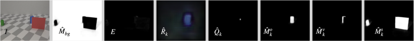
Figure 1: The inputs to the encoder of slot $k$ for one timestep, here depicting the blue object in the scene. Auto-regressive inputs are marked with a hat. From left to right: Current video frame, background mask, prediction error, reconstructed RGB slot image, Gaussian position map, object mask, visibility mask, and the summation of the visibility masks of the remaining slots.

3.2.2 Occlusion State

The introduction of the object mask enables Loci-Looped to determine the degree of occlusion for each object. We calculate the occlusion state $O^{t}_{k}$ as follows:

$$O^{t}_{k}=1-\frac{\sum_{i,j}[M^{t,v}_{k}(i,j)>\theta]}{\sum_{i,j}[M^{t,o}_{k}(i,j)>\theta]+c},$$ (2)

where $\theta$ is a threshold value, which we set to $0.8$, and $c$ is a small constant. By counting the number of pixels larger than threshold $\theta$, the denominator determines the total area of the object, while the numerator determines the visible area of the object. The occlusion state ranges from 0 (fully visible) to 1 (fully occluded), allowing Loci-Looped to explicitly represent the state of occlusion, increasing interpretability and serving as input to the percept gate controller.

3.2.3 Percept Gate

Loci-v1’s object tracking approach draws inspiration from Kalman filtering, which iteratively predicts object state changes and then adaptively fuses these predictions with current observations (Kalman, 1960). Similarly, Loci-v1 predicts the next object states, decodes them into pixel space and then uses these predictions along with the current frame to produce new object states (see Figure 2; outer loop). While the Kalman filter separates the steps of observation and information fusion, Loci-v1 observes and fuses jointly and implicitly in the encoding process. This is advantageous when fusing pixel-based information (e.g., combining hidden and visible object parts). However, when the model needs to fully maintain its own predictions because the current frame does not provide new information (e.g., during full occlusion), the encoding process becomes inefficient. Meanwhile, work from model-based reinforcement learning advocates the efficiency and precision of predicting directly in latent space (Hafner et al., 2019; 2020; Ha & Schmidhuber, 2018). Latent world models can be used to imagine how a scene will unfold while not being provided with new observations, fitting the problem of occlusion well. Therefore, we introduce an inner processing loop in Loci-Looped, which enables the model to propagate internal imaginations over time in latent space (see Figure 2; inner loop).

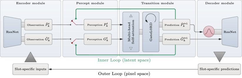
Figure 2: The slot-wise processing architecture of Loci-Looped. Predictions are made available on two routes. First, through an outer loop in pixel-space enabling consistent object tracking over time. Second, through an inner loop allowing for latent imaginations.

Similar to the Kalman filter, we equip the model with the ability to linearly interpolate between the current observations and the last predictions. Formally, the current object states $\smash{G^{t}_{k}}$, $\smash{P^{t}_{k}}$ become a linear blending of the observed object states $\smash{\tilde{G}^{t}_{k}}$, $\smash{\tilde{P}^{t}_{k}}$ and the predicted object states $\smash{\hat{G}^{t}_{k}}$, $\smash{\hat{P}^{t}_{k}}$:

$$G^{t}_{k}=\alpha^{t,G}_{k}\tilde{G}^{t}_{k}+(1-\alpha^{t,G}_{k})\hat{G}^{t}_{k}$$ (3)

$$P^{t}_{k}=\alpha^{t,P}_{k}\tilde{P}^{t}_{k}+(1-\alpha^{t,P}_{k})\hat{P}^{t}_{k}$$ (4)

The weighting $\alpha$ is specific for each Gestalt and position code in each slot $k$. Importantly, Loci-Looped learns to regulate this percept gate on its own in a fully self-supervised manner. It learns an update function $g_{\theta}$ which takes as input the observed state $\tilde{S}^{t}_{k}$, the predicted state $\hat{S}^{t}_{k}$, and the last positional encoding $P^{t-1}_{k}$:

$$(z_{k}^{t,G},z_{k}^{t,P})=g_{\theta}(\tilde{S}^{t}_{k},\hat{S}^{t}_{k},P^{t-1}_{k})+\varepsilon\hskip 36.135pt\text{with}\hskip 7.22743pt\varepsilon\sim\mathcal{N}(0,\Sigma),$$ (5)

where a state comprises the gestalt encoding, the positional encoding, and the occlusion state. By adding Gaussian noise with a fixed standard deviation $\Sigma$ to the function $g_{\theta}$, learning is biased to move further into plateaus away from ridges where possible. We model $g_{\theta}$ with a feed-forward network (see Appendix A.2.2). To be able to fully rely on its own predictions, Loci-Looped needs to be able to fully close the gate by setting $\alpha$ exactly to zero. We therefore use a rectified hyperbolic tangent to compute $\alpha$:

$$(\alpha^{t,G}_{k},\alpha^{t,P}_{k})=\mathrm{max}(0,\mathrm{tanh}((z_{k}^{t,G},z_{k}^{t,P}))).$$ (6)

To encourage robust world models without the reliance on continuous external updates, we impose an $L_{0}$ loss on gate openings (see Section 3.3) encouraging the sparse use of observations. The introduction of the percept gate enables Loci-Looped to control its perception flexibly fusing predictions with observations, essentially estimating their relative information values.

3.3 Training

We adopt the training procedure of Loci-v1. Loci-Looped is trained in a wholly unsupervised manner and undergoes end-to-end training, utilizing the rectified Adam optimization (Liu et al., 2021) in conjunction with truncated backpropagation through time (see Appendix A.2.4 for details). A complete list of the training losses used is presented in Table 1. Compared to Loci-v1, we dispense the use of an object permanence loss, which explicitly facilitated the maintenance of object representations in case of occlusions. Instead, Loci-Looped learns the concept of object permanence autonomously. Furthermore, it is worth noting that the percept gates do not only control the forward information flow, but also the backward flow of gradients. When the percept gates are closed, the error signal is thus only backpropagated to the transition module but not to the encoder module, which could lead to its degeneration. To avoid this, we incorporate a reconstruction loss in Loci-Looped that is directly derived from the current observations (see Appendix A.2.2 for details).

Table 1: Training losses used by Loci-v1 and Loci-Looped. Where $\mathrm{BCE}$ denotes the pixel-wise binary cross-entropy loss, $\mathrm{D}$ denotes the decoder, $p_{0}$ the image center and $\Theta$ the Heaviside function.

Loss	Term	Loci-v1	Loci-Looped
Next-Frame Prediction	$\mathrm{BCE}(I^{t+1},\mathrm{D}(\hat{G}^{t+1},\hat{P}^{t+1}))$	✓	✓
Gestalt Change Regularization	$\sum_{k}\bigl{[}\mathrm{D}_{k}(p_{0},G_{k}^{t})-\mathrm{D}_{k}(p_{0},\hat{G}_{k}^{t+1})\bigr{]}^{2}$	✓	✓
Position Change Regularization	$\sum_{k}\bigl{[}P_{k}^{t}-\hat{P}_{k}^{t+1}\bigr{]}^{2}$	✓	✓
Object Permanence Regularization	$\sum_{k}\bigl{[}D_{k}(P_{k}^{t},G_{k}^{t})-D_{k}(P_{k}^{t},\overline{G}_{k}^{t})\bigr{]}^{2}$	✓	-
Input-Frame Reconstruction	$\mathrm{MSE}(I^{t},\mathrm{D}(\tilde{G}^{t},\tilde{P}^{t}))$	-	✓
Gate Opening Regularization	$\sum_{k}(\Theta(\alpha^{t,G}_{k})+\Theta(\alpha^{t,P}_{k}))$	-	✓

4 Experiments and Results

In this section, we evaluate Loci-Looped with three main foci. We demonstrate that Loci-Looped reliably identifies objects and tracks them through occlusion. Second, it learns the concept of object permanence, anticipating the reappearance of occluded objects in VoE-like settings. Third, we show that Loci-Looped learns to deal with situations where visual data is temporarily missing.

4.1 Object Identification and Tracking

Dataset

We train on the ADEPT (Smith et al., 2019) dataset. The training set contains 1000 synthetic videos displaying up to 7 solid objects traversing the scene with constant speed and direction. The training set shows physically plausible dynamics including partial and full object occlusions, while excluding any other object interactions (e.g. collisions). We use 35 videos of the ADEPT vanish scenario as test set. This scenario starts with a large screen placed in the center of the scene. Then one or two objects enter the scene from opposite directions, disappear behind the screen, traverse the are behind the screen while hidden, reappear on the other side of screen, and finally exit the scene. The traversing objects are not visible for 10.3 frames on average which equals 25.0% of their total time being present.

Baselines

We compare Loci-Looped against Loci-v1 and SAVi (Kipf et al., 2022). Additionally, we perform an ablation experiment where we train a version of Loci-Looped with its percept gate deactivated, and we label this variant as Loci-Unlooped.

Metric

We evaluate the performance of the models with respect to two key capabilities. First, we quantify how well the models detect objects and identify them temporally consistent using the Multiple Object Tracking Accuracy (MOTA) (Bernardin & Stiefelhagen, 2008). Second, we quantify the model’s tracking error as the distance between estimated object positions and the true object positions. The estimated object positions can be easily extracted as Loci represents positional information explicitly. To extract object positions from the SAVi model, we first calculate object masks for each slot (see section 3.2.1) and then determine the center of these. Importantly, temporarily occluded objects are included in both metrics (see Appendix A.3 for details).

Results

The average tracking error and the MOTA are listed in Table 2. Loci-Looped outperforms both baseline models by a large margin. The fact that the tracking error hardly increases in occlusion, shows that Loci-Looped imagined the trajectory of hidden objects with high precision. At this point, we want to emphasize that this precision is remarkable given that Loci-Looped was never informed about the location or existence of objects. Importantly, $96.6\%$ of slots that were recruited before the occlusion phase achieved a final tracking error (i.e., the tracking error in the moment the objects exit the scene) smaller than $10\%$, indicating that these slots tracked their assigned objects successfully throughout the entire scene. The poor tracking results of Loci-Unlooped suggest that the internal loop is critical for successfully tracking objects through occlusions.

Table 2: Tracking results.

	Mean		Successful	MOTA	Mean
	Tracking Error (%)		trackings (%)		Gate Openings (%)
Model	Visible	Occluded	Overall	Overall	Visible	Occluded
Savi	26.7 $\pm$ 12.6	19.1 $\pm$ 9.8	3.2	-0.67	-	-
Loci-v1	12.5 $\pm$ 10.3	16.2 $\pm$ 7.5	38.4	-1.34	-	-
Loci-Unlooped	12.4 $\pm$ 14.8	7.7 $\pm$ 4.2	7.4	0.76	100 $\pm$ 0	100 $\pm$ 0
Loci-Looped	$\mathbf{2.6}$ $\pm$ 2.7	$\mathbf{2.7}$ $\pm$ 1.9	$\mathbf{96.6}$	$\mathbf{0.84}$	8.9 $\pm$ 11.7	0.8 $\pm$ 3.9

4.2 Object Permanence

Having seen that Loci-Looped tracks objects successfully through occlusion, we now test whether it has also learned to anticipate their reappearance.

Test scenario

We focus on the ADEPT’s vanish scenario that tests the concept of object permanence and inertia. The surprise condition (11 videos) features two objects but only one object reappears from behind the screen while the other vanishes while behind the screen. See Section 4.1 for the control condition. This scenario is designed to test the model’s anticipation about the reappearance of the occluded object.

Slot Error

To quantify an object- and thus slot-specific surprise we compute a slot error as follows:

$$E_{k}^{t}=\frac{\sum_{i,j}\bigl{[}(I^{t+1}-\hat{R}^{t+1})\odot\hat{M}_{k}^{t,v}\bigr{]}^{2}}{\sum_{i,j}\hat{M}_{k}^{t,v}},$$ (7)

where the overall prediction error is simply masked by the visibility mask of slot $k$. In addition, we divide the error by the sum of the visibility mask values to make the error invariant to the size of the object. For the following analysis we only consider slots that represent non-occluder objects and that achieved a final tracking error smaller than 10%.

Results

Loci-Looped maintains a clear object representation throughout the entire occlusion as illustrated in Figure 4. Moreover, we find that the model foresees the reappearance of occluded objects with high precision. As shown in Figure 3, the mean slot error spikes with the moment of expected reappearance. This is confirmed by a significant correlation between the slot error of vanished objects and the visibility of reappearing objects (frames: 25-40, $r(13)=.9,p<.001$). Likewise, we find the same pattern for the size of the visibility mask (frames: 25-40, $r(13)=.94,p<.001$), indicating that Loci-Looped expected the vanished objects to become visible again in this time period. Interestingly, we find a second peak of expectation in the moment the screen flips to the ground, failing to reveal the missing object.

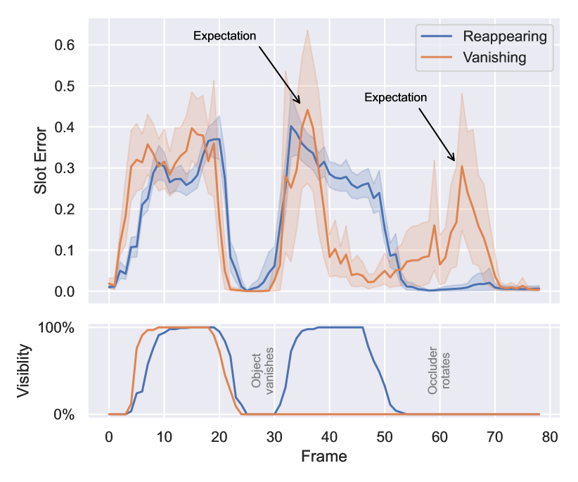
Figure 3: Results on the VoE experiment.

Further, we find that in the case of occlusion, Loci-Looped learned to close the percept gates, thus switching to a latent imagination mode (see Table 2). Similarly, we find that the model made onsly sparse usage of observations when objects were visible. This could explain the model’s learning of object permanence. By predicting the visible world while only glimpsing at it, the model essentially trained itself on simulated occlusions. Unlike real occlusions, this scheme provides access to targets and thus an error signal to learn from. This may have enabled the model to easily generalise to real occlusion scenarios where no sensations are available. In the next section, we test the model’s ability to handle temporary interruptions in sensory data.

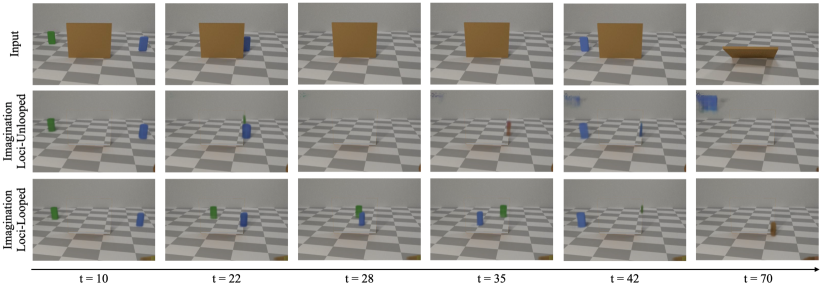
Figure 4: Surprise condition: Top row from left to right: Two objects traverse the scene, only one object reappears (blue), while the other vanishes (green). Middle row: Loci-Unlooped’s imagination on how the scene unfolds behind the occluder. Bottom row: Loci-Looped’s corresponding imagination indicating Loci-Looped surprise when the green object does not reappear on the right side. As a result, Loci-Looped attempts to keep an approximate imagination of it behind the occluder until the end of the sequence. The insight is possible by suppressing the occluder-slot during decoding.

4.3 Sensory Interruptions

Having seen that Loci-Looped can handle the representation of partially observable scenes, we now investigate how it behaves when no observation is available for a brief period of time, simulating a short blink.

Dataset

The CLEVRER dataset (Yi et al., 2020) contains 10,000 videos showing up to 6 small objects moving through a scene, including collisions and partial occlusions. Again, we increase the video speed by considering only every second frame resulting in 64 frames per video. We make use of the training and testing split provided by Wu et al. (2023b).

Sensory Interruptions

In training and testing, we simulate sensory interruptions by setting the current input image to black with a probability of 20%. During such blackouts, the models are thus required to maintain a stable scene representation without input information. They thus can only imagine how the scene will unfold. In the first 10 frames of each sequence we do not allow blackouts.

Metric

We evaluate the next-frame prediction quality using PSNR, SSIM (Wang et al., 2004), and LPIPS (Zhang et al., 2018). In addition, we assess the segmentation quality using the Average Recall (AR), the Adjusted Rand Index (ARI), a foreground specific ARI (FG-ARI) and a foreground specific intersection over union (FG-mIoU). We use the stochastic SAVi implementation as well as the evaluation scripts provided by (Wu et al., 2023b).

Results

As depicted in Table 3, Loci-Looped demonstrates superior performance compared to SAVi and Loci-Unlooped in timesteps with no available input frames and in timesteps with provided input frames. This observation implies that only Loci-Looped can consistently uphold stable object representations during blackout periods, whereas the baseline models strongly depend on uninterrupted sensory input, which is also illustrated in Figure 5.

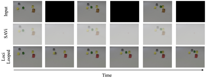
Figure 5: Visual results of the sensory interruptions experiment on the CLEVRER dataset.

Table 3: Results on the Sensory Interruptions experiment on the CLEVRER Dataset.

Input	Method	PSNR	SSIM	LPIPS $\downarrow$	AR	ARI	FG-ARI	FG-mIoU
Blackout	SAVi	25.3	0.81	0.47	0.0	0.0	0.01	0.01
	Loci-Unlooped	21.8	0.71	0.47	0.0	0.0	0.02	0.01
	Loci-Looped	$\mathbf{34.6}$	$\mathbf{0.95}$	$\mathbf{0.11}$	$\mathbf{0.88}$	$\mathbf{0.86}$	$\mathbf{0.78}$	$\mathbf{0.42}$
Visible	SAVi	$\mathbf{37.5}$	0.96	0.19	0.47	0.57	$\mathbf{0.90}$	0.36
	Loci-Unlooped	28.1	0.86	0.26	0.38	0.46	0.38	0.20
	Loci-Looped	36.3	$\mathbf{0.97}$	$\mathbf{0.10}$	$\mathbf{0.92}$	$\mathbf{0.88}$	0.81	$\mathbf{0.43}$

5 Discussion

In this work, we introduced Loci-Looped: an object-centric world model that has the ability to flexibly fuse outer loop sensations with inner loop imaginations into a consistent percept. Loci-Looped tracks objects through occlusion, learns the physical concepts of object permanence and inertia from scratch, and is robust to interruptions in its sensory signal. It builds on the idea that objects can not only be leveraged to decompose a scene but also to assemble a scene percept from object-wise observations (e.g., visible objects) as well as object-wise imaginations (e.g., occluded objects). Importantly, all of this was learned without supervision, without access to a temporal buffer, and solely from the next-frame prediction objective. In line with Piloto et al. (2022), our work suggests that intuitive physics may emerge from learning an anticipatory world model that constantly predicts future world states.

Future advancements of Loci-Looped should incorporate probabilistic scene representations. As shown in Smith et al. (2019), probabilistic transition models are advantageous for building expectations in scenarios featuring agentive elements in more complicated VoE scenarios than the one presented in this work. This is especially the case for scenarios in which the agent acts while being occluded (e.g., an object that actively halts behind an occluder), which are often featured in more complicated VoE scenarios than the one presented in this work. Furthermore, improving the learning of complex object interactions beyond containment, such as collisions, in a history-compressing architecture, such as the introduced Loci-Looped, will need to be examined in further detail.

In conclusion, this work contributes to the growing body of research demonstrating the potential of compositional scene representations for achieving more human-like scene understanding and modelling cognitive development in artificial intelligence systems (Wu et al., 2023b; Locatello et al., 2020; Yuan et al., 2023; Piloto et al., 2022; Traub et al., 2023; Weihs et al., 2022). We believe that the introduced adaptive information fusion process can be easily integrated into other compositional scene segmentation algorithms. Overall, we hope that the presented algorithms and enhancements will contribute to further advance the development of more human-like visual intelligence and conceptual cognition, generally speaking.

6 Acknowledgement

This work received funding from the Deutsche Forschungsgemeinschaft (DFG, German Research Foundation) under Germany’s Excellence Strategy – EXC number 2064/1 – Project number 390727645 as well as from the Cyber Valley in Tübingen, CyVy-RF-2020-15. The authors thank the International Max Planck Research School for Intelligent Systems (IMPRS-IS) for supporting Manuel Traub, and the Alexander von Humboldt Foundation for supporting Martin Butz and Sebastian Otte.

Appendix A Appendix

The Appendix provides additional information on the method A.2 and the results A.5.

A.1 Related Work

Recently, two studies in the field of intuitive physics have gained attention for introducing a VoE dataset and models that learn the concepts of permanence, solidity, and continuity. Similiar to Loci-Looped, the Physics Learning through Auto-encoding and Tracking Objects (PLATO) model (Piloto et al., 2022) uses a slot-wise encoder-predictor architecture. The second model is the Approximate Derendering Extended Physics and Tracking (ADEPT) model (Smith et al., 2019) which implements a hand-crafted physical reasoning system. In this section, we will review both approaches and compare them with Loci-Looped.

Representation Loci-Looped, PLATO and ADEPT model physics at the level of objects. To incorporate this object-centric approach all models make use of a slot architecture, where a slot represents a processing pipeline dedicated to a single object. This slot-based architecture enables the parallel processing of multiple objects, applying the same model by weight sharing. The models differ in their latent code constraints. While PLATO does not constrain the latent code at all, ADEPT explicitly encodes the object’s type, location, velocity, rotation, scale and color. As Smith et al. (2019) has shown, this abstract encoding is beneficial for generalising to unseen objects, but requires supervised training. Balancing both approaches and inspired by the dorsal and ventral visual processing stream in humans, Loci-Looped disentangles an object’s position (where) and gestalt (what).

Segmentation To identify objects in an image PLATO relies on ground-truth segmentation masks, while ADEPT uses a supervised segmentation network. Unsupervised methods for image segmentation typically learn to decompose scenes into object-centric representations using slot-wise autoencoders (Burgess et al., 2019; Greff et al., 2020). Similarly, Loci-Looped learns to identify objects in a scene using a slot-wise encoder-decoder architecture. By encoding positional information explicitly and constraining the gestalt encoding capacity, each slot is naturally biased towards representing a cohesive and uniform area of the image. While Loci-v1 is capable of segmenting scenes with complex backgrounds using an additional high-capacity background slot (Traub et al., 2023), this feature requires intensive training on the background. Our work focuses on short scenes with varying backgrounds, making it necessary to provide the model with the background for each scene.

Dynamics Modelling All three models leverage a dynamics module to estimate the state of the objects at the next timestep. While ADEPT does not learn objects dynamics but utilizes an out-of-the-box physics engine for this purpose, Loci-Looped and PLATO make use of recurrent units. In PLATO, a slot-wise LSTM is combined with two feedforward networks accounting for pairwise object interactions to model object dynamics. Loci-Looped differs with respect to the choice of the recurrent unit and how interactions are modelled. Loci-Loopeduses a slot-wise GateLORD (Gumbsch et al., 2022) module that penalizes latent state changes and thereby fosters stable hidden object state representations over time, while interactions between objects is modelled using multi-head self-attention between slots.

Tracking Accurately identifying objects over time is crucial for estimating and predicting object motion. In practice, this means that recurrent prediction slots must receive consistent information about the same object over time to enable reliable predictions. To achieve this, PLATO relies on ground-truth information, while ADEPT utilizes a hand-crafted observation model that matches objects in the current observation with objects in the model’s belief based on extracted object features. Similar, recent research has proposed an alignment module that learns to match object encodings between observations and a memory (Creswell et al., 2021). A different approach is taken by Loci-Looped. The encoder module learns to consistently parse the same object in the same slot via a predictive coding approach, which yield the to-be-minimized reconstruction error of the previous time step as additional input. Moreover, each slot of the encoder receives its previous output, thus priming its particular object-encoding responsibility. Finally, the internal GateLORD units as well as a time persistence loss further encourage latent encodings of the same object properties in the same slot over time.

Temporal memory To predict the next position of objects, the models have to consider their movements. To do so, ADEPT’s supervised perception module receives a history of three images and derives object velocities from it. In contrast, the recurrence in the dynamics modules of PLATO and Loci-Looped allows to accumulate information over time and thus to capture object dynamics in the cell states. Although theoretically not needed, PLATO makes its prediction based on all past object encodings stored in an object buffer which is also used to derive object interactions. On the other hand, Loci-Looped’s dynamic module predicts the next object state based solely on the current object state, requiring it to fully capture object dynamics within the current cell state.

Object permanence The ADEPT model does not learn object permanence which is by default built into the physics engine. In contrast, PLATO learns to predict the reappearance of hidden objects, which is however favored by access to the full history of object codes, informing about the previous existence of the object, and by a relative short duration of occlusion.

A.2 Method

A.2.1 Object Mask

In practice, the object mask proved particularly useful in two scenarios. First, when objects slide into occlusion. To produce full-extent encodings of these objects the encoder has to combine information from the input image depicting visible parts and information from the predicted RGB reconstruction depicting occluded parts. The object mask helps the encoder to do so by marking the full shape of the object. Second, when objects slide out of occlusion. In this scenario, the visibility mask is only helpful if the time of reappearance is predicted precisely, otherwise it will be empty. In contrast, the object mask can still provide useful information by indicating that an object is close to reappearing.

A.2.2 Percept Gate Controller

The percept gate controller is part of the slot-wise gate module and computes $\alpha_{k}^{t,G}$ and $\alpha_{k}^{t,P}$. The controller receives the inputs $\tilde{P}^{t}_{k}$, $\tilde{G}^{t}_{k}$, $\tilde{O}^{t}_{k}$, $\hat{P}^{t}_{k}$, $\hat{G}^{t}_{k}$, $\hat{O}^{t}_{k}$, $\hat{P}^{t-1}_{k}$ which are concatenated into a vector of size 206. This vector is then fed into a feed-forward network modelling update function $g_{\theta}$. This network is composed of three linear layers with dimensions 32, 16, and 2, and employs the hyperbolic tangent activation function. During the training phase, the network’s output is augmented with Gaussian noise ($\Sigma=0.1$); however, this is not applicable during the inference stage. As demonstrated by Gumbsch et al. (2022), the stochastic component fosters the learning of sparse gate openings. The final values for $\alpha^{t,G}_{k}$ and $\alpha^{t,P}_{k}$ are calculated using the rectified hyperbolic tangent function ($\Lambda$). The rectified variant generates values within the range $[0,1)$, thus enabling the model to fully close the gates (i.e., $\alpha=0$). In the backward propagation, the following pseudo-derivative is employed:

$$\Lambda^{\prime}=\frac{\partial\Lambda(x)}{\partial x}=\begin{cases}0&\text{if }x\leq 0\\ (1-\Lambda(x)^{2})&\text{otherwise}\end{cases}$$ (8)

In addition, we penalize gate openings (i.e. $\alpha>0$) by applying a $L_{0}$ regularization. We therefore use the method described in Gumbsch et al. (2022). The regularization loss is given as the sum of gate openings:

$$L_{\textrm{Gate}}=\sum_{k}(\Theta(\alpha^{t,G}_{k})+\Theta(\alpha^{t,P}_{k})),$$ (9)

where $\Theta$ is the non-differentiable Heavisite step function. We therefore use the derivative of the linear function as the pseudo-derivative:

$$\Theta^{\prime}=\frac{\partial\Theta(x)}{\partial x}=1.$$ (10)

A.2.3 Slot Recruiting

A crucial step in slot-based architectures is the initial assignment of slots to objects. Traub et al. (2023) demonstrated that Loci-v1 can allocate multiple slots in parallel to identify multiple objects. However, this allocation scheme can be sensitive to object sizes. Specifically, large objects are more complicated to reconstruct than small objects and thus provoke larger prediction errors. As a consequence large objects tend to attract multiple slots in parallel, resulting in one object being encoded partly in multiple slots. To encourage the representation of entire objects in exclusively one slot, we restrict the encoder to only use one slot at a time seeking for new objects. In general, we distinguish between occupied slots which already represent an object and empty slots which do not represent an object yet. Once both the visibility masks $\tilde{M}_{k}^{t+1,v}$ and $\hat{M}_{k}^{t+1,v}$ exceed a threshold of 0.8 in one pixel, the corresponding slot is marked as occupied for the entire sequence. At the start of a sequence Loci-Looped has one empty slot available. When this empty slot becomes occupied a new one is recruited with a delay of two timesteps. This delay allows the initial slot to encode the object in its entirety. This pattern repeats when the empty slot becomes occupied again. In addition, every second frame the isotropic Gaussian $\hat{Q}^{t}_{k}$ of the empty slot is set to the position $(x,y)$ of the largest prediction error in the background i.e.

$$(x,y)=\operatorname*{argmax}_{(i,j)}\ (M_{bg}\odot E)(i,j)$$ (11)

before entering the encoding process. With this incremental recruiting scheme, Loci-Looped encodes entire objects of varying sizes more reliably in one slot.

A.2.4 Training procedure

The training procedure entails randomly selecting sequences from the dataset and compiling them into a single batch. This batch is then processed sequentially, with the model ingesting consecutive frames and executing a backward pass every $n$ frames. Simultaneously, an optimizer step is conducted every $n$ frames, followed by the detachment of gradients. Only the internal hidden states remain unaltered, and they are cleared only after the full batch of sequences has been processed. Similarly, the eprop eligibility traces employed within the GateL0rd layers are maintained for each sequence. It is important to highlight that these eligibility traces effectively facilitate the integration of error information from the past beyond the truncation horizon of backpropagation-through-time by accumulating previous neuron activations, akin to the approach described in Bellec et al. (2019) which facilities the the learning of long lasting memory states as previously demonstrated by Traub et al. (2023).

Training the model in an unsupervised fashion is challenging which requires increasing the difficulty of the task in three phases. During the first phase, the focus is on learning to represent foreground objects. Therefore, the reconstruction and the prediction loss are initially only applied to the foreground by masking the corresponding targets,

$$I^{t\prime} =I^{t}\odot M^{t}_{fg}+I^{t}\odot(1-M^{t}_{fg})\cdot\beta$$ (12)

$$M^{t}_{fg} =\theta<(I^{t}-I^{t}_{bg})^{2},$$ (13)

where $\beta$ is set to zero. To encourage initial slot bindings, all slots are placed in parallel and in a stochastic fashion to the largest foreground errors. By the end of the first phase, the model should be able to use the slots to rudimentarily reconstruct and predict the foreground. In the second training phase the aim is to learn to represent entire objects in one slot, for which slot recruiting (see Section A.2.3) is enabled. In addition, the background is blended in the losses by gradually increasing $\beta$ to one. This enforces the learning of background mask $M_{bg}$ which is used to distinguish between background and foreground. At the end of phase two, the model should be able to reconstruct and predict complete scenes. Until this point, the update module was skipped focusing the training on the outer loop and visible objects. This is changed in the last training phase, in which the update module is enabled and the model’s imagination is trained. Loci-Looped then learns to balance information from the inner and the outer loop.

A.2.5 Teacher forcing

Following (Traub et al., 2023), Loci-Looped starts a sequence by repeatedly processing the first frame $x$ times (teacher forcing phase). The prediction target is given by first frame as well. This allows the model to identify initial objects in the scene using slot recruiting. In this phase the updatemodule and transition module are skipped, basically using the encoder and decoder module as slot-wise auto-encoder for an initial scene segmentation.

A.2.6 Training specifics

From 200k updates on wards we summed the gradients over two timesteps and then ran one joint optimization step. In addition, we applied a dropout on the prediction error $E_{t}$ before entering the encoder ($p=0.1$).

Table 4: Loci Training Specifics

Paramater	ADEPT	CLEVRER
Learning Rate	$1\cdot 10^{-4}$	$1\cdot 10^{-4}$
Learning Rate (from 400k updates)	$3.3\cdot 10^{-5}$	$3.3\cdot 10^{-5}$
Batch size	16	32
Number of updates	1150000	800000
Teacher forcing length	10	10
Resolution	120x80	120x80
Resolution (from 600k updates)	480x320	120x80
Number slots (objects)	7	6
Start training phase 2	30k updates	30k updates
Start training phase 3	60k updates	60k updates
GateLORD Regularization	$1\cdot 10^{-10}$	$1\cdot 10^{-10}$
Video length (training)	41 frames	64 frames
Training set size	1000	20000
Frame offset	3 frames	2 frames

A.3 Object Identification and Tracking

A.3.1 Training Set

Each video contains a different background and a static camera perspective. We used 90% of videos for training and 10% for validation. In addition, we increased the video speed by considering only every third frame, which gives a video length of 41 frames. We trained 3 independent models of Loci-Looped for the ADEPT dataset and averaged the results across slots. For the other models and the CLEVRER dataset we only trained one model.

A.3.2 Tracking Error

Loci-Looped encodes object positions explicitly in 2D image coordinates which is highly interpretable, allowing us to easily quantify the model’s tracking precision as the distance between estimated object positions and the true object positions. To do so, we pair the models internal representations with the ground-truth objects in the scene. More specifically, each time the model detects a new object the current positional encoding is used to assign the slot to the closest object in the scene based on euclidean distance. This pairing is then locked. Finally, at each timestep the slot-specific tracking error $T^{t}_{k}$ is computed as the euclidean distance between the estimated and the true object position. Lastly, we scale the error to the interval 0 to 1 by dividing the error by the image diagonal $d$:

$$T^{t}_{k}=\frac{\sqrt{(\hat{P}_{k}^{t}-P_{o}^{t})^{2}}}{d},$$ (14)

where $P_{o}^{t}$ is the true position of the assigned object.

A.3.3 Multiple Object Tracking Accuracy

In addition, we record the Multiple Object Tracking Accuracy (MOTA) (Bernardin & Stiefelhagen, 2008) to quantify how well the model detects objects and identifies them temporally consistent. The MOTA is given as:

$$\mathrm{MOTA}=1-\frac{\sum_{t}(\mathrm{FN}_{t}+\mathrm{FP}_{t}+\mathrm{IDS}_{t})}{\sum_{t}\mathrm{GT}_{t}},$$ (15)

where FN denotes the number of false negative detections, FP the number of false positive detections, IDS the number of object switches between slots, and GT the true object instances. Each timestep the ground-truth objects in the scene are paired with the slot representations based on euclidean distance (see Appendix A.3.2). As this is a one-to-one mapping, MOTA counts unassigned slots as false-positives and unassigned objects as false-negatives. Object switches occur if an object is first assigned to slot a and later to slot b. Importantly, we also provide the position of occluded objects as part of GT.

We used the python package motmetrics for computing the MOTA (https://github.com/cheind/py-motmetrics). Pairwise distances between slot positions and ground-truth positions were calculated using euclidean distance, where the cutoff distance was set to 10% of the image diagonal. Further, we only considered occupied slots (see Section A.2.3) which, made a position estimate within the image borders, and predicted their slot-object to exist ($\sum_{(i,j)}(\hat{M}^{t,o}_{k})>100$, i.e. the object mask size exceeds a threshold of 100).

A.4 SAVi Training

For training SAVi Kipf et al. (2022), we used the stochastic SAVi implementation as well as the hyper-parameters provided by Wu et al. (2023b). We used a resolution of 64x64 for both the ADEPT and the CLEVRER dataset. For training efficiency (see (Wu et al., 2023b)) we trained SAVi on subsequences of the full videos which had length 6. For the ADEPT dataset, we trained SAVi for 4 epochs, for longer training we observed that the model overfitted to the background and started to neglect foreground objects. For the CLEVRER dataset, we trained SAVi for 12 epochs including simulated blackouts in the training.

A.5 Results

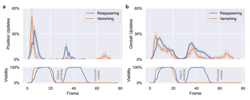
Figure 6: Gate openings on the Violation of Expectation experiment. Traversing objects either reappear from occlusion (blue) or vanish in occlusion (red). Finally, the occluder rotates to the ground providing full insight to the scene.

Appendix B Loci-Looped Algorithm

In the remainder, we denote scalar values by lower-case letters, tensors by upper-case letters, and vectors by bold letters. Moreover, we denote slot-specific activities with a subscript $k\in{1,..,K}$ and time by the superscript $t$. We drop $t$ for temporary values.

B.1 Slot-wise encoder

Inputs

The encoder inputs at each time step $t$ consist of:

• RGB input image $I^{t}\in\mathbb{R}^{H\times W\times 3}$,

• MSE map $E^{t}\in\mathbb{R}^{H\times W\times 1}$ (pixel-wise mean squared error between $I^{t}$ and $\hat{R}^{t}$),

• Slot-specific RGB image reconstructions $\hat{R}^{t}_{k}\in\mathbb{R}^{H\times W\times 3}$,

• Slot-specific visibility mask predictions $\hat{M}^{t,v}_{k}\in\mathbb{R}^{H\times W\times 1}$,

• Slot-specific visibility mask complements $\hat{M}^{t,s}_{k}=\sum_{k^{\prime}\in\{1,..,K\}\setminus k}\hat{M}^{t,v}_{k^{\prime}}$

• Slot-specific object mask predictions $\hat{M}^{t,o}_{k}\in\mathbb{R}^{H\times W\times 1}$,

• Slot-specific isotropic Gaussian position map predictions $\hat{Q}^{t}_{k}\in\mathbb{R}^{H\times W}$,

• Background mask $\hat{M}^{t}_{bg}\in\mathbb{R}^{H\times W}$, which is equivalent to $1-\sum_{k\in\{1,..,K\}}\hat{M}^{t}_{k}$

Outputs

Based on these inputs, the slot-wise encoder network generates latent codes:

• Slot-specific Gestalt codes $\tilde{G}^{t}_{k}\in\mathbb{R}^{D_{g}}$,

• Slot-specific position codes $\tilde{P}^{t}_{k}\in\mathbb{R}^{4}$ encode an isotropic Gaussian $(\boldsymbol{\mu}^{t}_{k},\sigma^{t}_{k})$ and a slot-priority code $z^{t}_{k}$,

where $D_{g}$ denotes the size of the Gestalt code and $\boldsymbol{\mu}^{t}_{k}\in\mathbb{R}^{2}$.

B.2 Slot-wise decoder - reconstruction

Inputs

The outputs of all slots from the encoding module $\tilde{P}^{t}$ and $\tilde{G}^{t}$ then act as the input to the decoder.

Outputs

The output of the decoder includes the slot-respective masks and RGB reconstructions:

• Slot-specific visibility mask outputs $\tilde{M}^{t,v}_{k}\in\mathbb{R}^{H\times W}$,

• Slot-specific object mask outputs $\tilde{M}^{t,o}_{k}\in\mathbb{R}^{H\times W}$,

• Slot-specific RGB image reconstructions $\tilde{R}^{t}_{k}\in\mathbb{R}^{H\times W\times 3}$,

Further, we compute the slot-specific occlusion state $\tilde{O}^{t}_{k}$ as a function of $\tilde{M}^{t,v}_{k}$ and $\tilde{M}^{t,o}_{k}$, as specified in Equation 2. We generate the combined reconstructed image $\hat{R}^{t}$ by summing all slot reconstructions $\tilde{R}^{t}_{k}$ and the background estimate $\tilde{R}_{bg}$ weighted with their corresponding masks $\tilde{M}^{t}_{k}$ and $\tilde{M}^{t}_{bg}$, as specified further in Algorithm 1. The reconstructed image $\hat{R}^{t}$ is subject to the reconstruction loss (see Equation LABEL:eq:reconstructionloss) and the occlusion state $\tilde{O}^{t}_{k}$ serves as input to the update gate controller.

B.3 Update module

The slot-wise update module consists of an update gate controller and an update gate. The update gate controller takes the inputs,

• Slot-specific encoder Gestalt codes $\tilde{G}^{t}_{k}\in\mathbb{R}^{D_{g}}$,

• Slot-specific encoder position codes $\tilde{P}^{t}_{k}\in\mathbb{R}^{4}$,

• Slot-specific encoder occlusion state $\tilde{O}^{t}_{k}\in\mathbb{R}^{D_{g}}$,

• Slot-specific predicted Gestalt codes $\hat{G}^{t}_{k}\in\mathbb{R}^{D_{g}}$,

• Slot-specific predicted position codes $\hat{P}^{t}_{k}\in\mathbb{R}^{4}$,

• Slot-specific predicted occlusion state $\hat{O}^{t}_{k}\in\mathbb{R}^{D_{g}}$,

• Slot-specific previous position codes $P^{t-1}_{k}\in\mathbb{R}^{4}$

and outputs gate activation:

• Slot-specific Gestalt gate activation $\alpha^{t,G}_{k}\in[0,1)$,

• Slot-specific position gate activation $\alpha^{t,P}_{k}\in[0,1)$.

The update gate then linearly interpolates between $\tilde{G}^{t}_{k}$ and $\hat{G}^{t}_{k}$, as well as $\tilde{P}^{t}_{k}$ and $\hat{P}^{t}_{k}$, where a higher activation opens the gate and gives more weighting to $\tilde{G}^{t}_{k}$ or $\tilde{P}^{t}_{k}$. Finally, the update module produces:

• Slot-specific Gestalt codes $G^{t}_{k}\in\mathbb{R}^{D_{g}}$,

• Slot-specific position codes $P^{t}_{k}\in\mathbb{R}^{4}$,

B.4 Transition module

A transition module is used to process interaction dynamics within and between these slot-respective codes and creates a prediction for the next state, which is fed into the decoder. The input to the transition module equals $G_{k}^{t}$, $P_{k}^{t}$, $\alpha^{t,G}_{k}$ and $\alpha^{t,P}_{k}$. It is processed across slots and per slot in the respective layers: Multi-Head Attention predicts slot interactions (across slots), while GateL0RD predicts slot-specific dynamics (per slot). We use two attention layers with ten heads each with GateL0RD layers in between.

Outputs

The outputs of the transition module $\hat{G}^{t+1}_{k}$ and $\hat{P}^{t+1}_{k}$ have the same size as $G^{t}_{k}$ and $P^{t}_{k}$. Additionally, recurrent, slot-respective hidden states $\hat{H}^{t}_{k}$ are maintained in the time-recurrent GateL0RD layers:

• Slot-specific position codes $\hat{P}^{t+1}_{k}\in\mathbb{R}^{4}$,

• Slot-specific Gestalt codes $\hat{G}^{t+1}_{k}\in\mathbb{R}^{D_{g}}$,

• Slot-specific GateL0RD-layer-respective hidden states $\hat{H}^{t}_{k}\in\mathbb{R}^{D_{h}}$,

where $D_{h}$ denotes the size of the recurrent latent states.

B.5 Slot-wise decoder - prediction

Inputs

The outputs of all slots from the transition module $\hat{P}^{t+1}$ and $\hat{G}^{t+1}$ then act as the input to the decoder.

Outputs

The output of the decoder includes the slot-respective masks and RGB reconstructions:

• Slot-specific visibility mask outputs $\hat{M}^{t+1,v}_{k}\in\mathbb{R}^{H\times W}$,

• Slot-specific object mask outputs $\hat{M}^{t+1,o}_{k}\in\mathbb{R}^{H\times W}$,

• Slot-specific RGB image reconstructions $\hat{R}^{t+1}_{k}\in\mathbb{R}^{H\times W\times 3}$,

which are then used as part of the input at the next iteration as specified above. Further, we compute the slot-specific occlusion state $\hat{O}^{t}_{k}$ as a function of $\hat{M}^{t+1,v}_{k}$ and $\hat{M}^{t+1,o}_{k}$, as specified in 2.

We generate the combined reconstructed image $\hat{R}^{t+1}$ by summing all slot estimates $\hat{R}^{t+1}_{k}$ and the background estimate $\hat{R}_{bg}$ weighted with their corresponding masks $\hat{M}^{t+1}_{k}$ and $\hat{M}^{t+1}_{bg}$, as specified further in Algorithm 1. The predicted image $\hat{R}^{t+1}$ is subject to the prediction loss (see LABEL:eq:reconstructionloss) and the occlusion state $\tilde{O}^{t+1}_{k}$ serves as input to the update gate controller in the next timestep.

Algorithm 1 Loci-v2-Algorithm (main processing loop)

1:  Inputs: Input video $I\in\mathbb{R}^{T\times H\times W\times 3}$, static background $\hat{R}_{bg}\in\mathbb{R}^{H\times W\times 3}$

2:  Network parameters: $\Theta_{encoder}$, $\Theta_{update}$, $\Theta_{transition}$, $\Theta_{decoder}$

3:  Additional parameters: initialization parameters $\Theta_{init}$; background threshold $\theta_{bg}$, which is encoded as a uniform offset mask $\tilde{M}_{bg}\leftarrow\theta_{bg}$; number of slots $K$; processing steps $T$

4:  Initialize $H_{k}^{1},\hat{R}^{1}_{k},\hat{R}^{1},\hat{M}^{1,o}_{k},\hat{M}^{1,v}_{k},\hat{Q}^{1}_{k}$

5:  for $t=1\dots T$ do

6:     COMMENT# Pre-processing:

7:     $E^{t}\leftarrow\sqrt{\texttt{Mean}\left(\left(I^{t}-R_{bg}\right)^{2},axis=\text{'rgb'}\right)}\circ\sqrt[4]{\texttt{Mean}\left(\left(I^{t}-\hat{R}^{t}\right)^{2},axis=\text{'rgb'}\right)}$

8:     compute complement $\hat{M}^{t,s}_{k}$

9:     COMMENT# Slot-wise encoder:

10:     $S^{t}_{k}\leftarrow Encoder_{Trunk}(I^{t},E^{t},\hat{R}^{t}_{k},\hat{M}^{t,v}_{k},\hat{M}^{t,o}_{k},\hat{M}^{t,s}_{k},\hat{Q}^{t}_{k},\hat{M}_{bg}^{t})$

11:     $\tilde{G}^{t}_{k}\leftarrow Encoder_{Gestalt}(S^{t}_{k})$

12:     $P^{\prime t}_{k}\leftarrow Encoder_{Position}(S^{t}_{k})$

13:     $\tilde{P}^{t}_{k}\leftarrow\texttt{concat}\left[\boldsymbol{\mu}^{t}_{k},\sigma^{t}_{k},z^{t}_{k}\right]\leftarrow\texttt{concat}\left[Encoder_{\boldsymbol{\mu}}(P^{\prime t}_{k}),Encoder_{\boldsymbol{\sigma}}(P^{\prime t}_{k}),Encoder_{z}(P^{\prime t}_{k})\right]$

14:     COMMENT# Slot-wise decoder - reconstruction (see decoder - prediction and post-processing):

15:     $\tilde{O}^{t}_{k}\leftarrow 1-\frac{\sum_{i,j}[\tilde{M}^{t,v}_{k}(i,j)>\theta_{bg}]}{\sum_{i,j}[\tilde{M}^{t,o}_{k}(i,j)>\theta_{bg}]+0.0001}$

16:     $\tilde{R}^{t}\leftarrow\texttt{sum}(\texttt{concat}\left[\tilde{R}^{t}_{1},..,\tilde{R}^{t}_{K},\tilde{R}_{bg}\right]\circ\tilde{M}^{t,v},axis=\text{'K'})$

17:     COMMENT# Update module:

18:     $[\alpha^{t,G}_{k},\alpha^{t,P}_{k}]\leftarrow UpdateController(\tilde{P}^{t}_{k},\tilde{G}^{t}_{k},\tilde{O}^{t}_{k},\hat{P}^{t}_{k},\hat{G}^{t}_{k},\hat{O}^{t}_{k},P^{t-1}_{k})$

19:     $G^{t}_{k}\leftarrow\alpha^{t,G}_{k}\tilde{G}^{t}_{k}+(1-\alpha^{t,G}_{k})\hat{G}^{t}_{k}$

20:     $P^{t}_{k}\leftarrow\alpha^{t,P}_{k}\tilde{P}^{t}_{k}+(1-\alpha^{t,P}_{k})\hat{P}^{t}_{k}$

21:     COMMENT# Transition module:

22:     $\hat{G}^{t+1},\hat{P}^{t+1},H^{t+1}=TransitionModule(G^{t},P^{t},\alpha^{t,G}_{k},\alpha^{t,P}_{k},H^{t})$

23:     COMMENT# Gestalt binarization:

24:     $\hat{G}^{t+1}\leftarrow\texttt{Sigmoid}(\hat{G}^{t+1})$

25:     $\hat{G}^{t+1}\leftarrow\hat{G}^{t+1}+\hat{G}^{t+1}(1-\hat{G}^{t+1})\mathcal{N}(0,1)$

26:     COMMENT# Slot-wise decoder - prediction:

27:     COMMENT# $p$ encodes all pixel positions normalized to $[-1,1]$, width the number of pixels in a row

28:     $\hat{Q}^{t+1}_{k}\leftarrow\exp\left(\frac{-(p-\hat{\boldsymbol{\mu}}^{t+1}_{k})^{2}}{2\max\left(\frac{1}{\texttt{width}},\hat{\sigma}^{t+1}_{k}\right)^{2}}\right)$

29:     $decode_{k}\leftarrow\texttt{Priority-Based-Attention}(\hat{G}^{t+1}_{k},\hat{Q}^{t+1}_{k},\hat{\mathbf{z}}^{t+1})$

30:     $\hat{R}^{t+1}_{k},\tilde{M}^{t+1}_{k}\leftarrow Decoder_{Trunk}(decode_{k})$

31:     COMMENT# Post-processing:

32:     $[\hat{M}^{t+1,v}_{1},\dots,\hat{M}^{t+1,v}_{K},\hat{M}^{t+1}_{bg}]\leftarrow\texttt{softmax}(\texttt{concat}[\tilde{M}^{t+1}_{1},\dots,\tilde{M}^{t+1}_{K},\tilde{M}_{bg}],axis=\text{'K'})$

33:     $\hat{M}^{t+1,o}_{k}\leftarrow\frac{\mathrm{exp}(\hat{M}^{t+1}_{k})}{\mathrm{exp}(\hat{M}^{t+1}_{k})+\mathrm{exp}(\hat{M}^{t+1}_{bg})},$

34:     $\hat{O}^{t+1}_{k}\leftarrow 1-\frac{\sum_{i,j}[\hat{M}^{t+1,v}_{k}(i,j)>\theta_{bg}]}{\sum_{i,j}[\hat{M}^{t+1,o}_{k}(i,j)>\theta_{bg}]+0.0001}$

35:     $\hat{R}^{t+1}\leftarrow\texttt{sum}(\texttt{concat}\left[\hat{R}^{t+1}_{1},..,\hat{R}^{t+1}_{K},\hat{R}_{bg}\right]\circ\hat{M}^{t+1,v},axis=\text{'K'})$

36:  end for

37:  return $[\hat{R}^{1}\dots\hat{R}^{T}]$

Algorithm 2 Priority-based-Attention

1:  Inputs: Gestalt: $G_{k}\in\mathbb{R}^{1,D_{g}}$, Gaussian 2d position: $Q_{k}\in\mathbb{R}^{H^{\prime}\times W^{\prime}\times 1}$, priority: $\boldsymbol{z}\in\mathbb{R}^{K}$

2:  Additional parameters: values of the learnable $\boldsymbol{\theta^{w}}\in\mathbb{R}^{K}$ are initially set to $25$, while $\boldsymbol{\theta^{b}}\in\mathbb{R}^{K}=\{0,1,\dots,(K-1)\}$ induces a default slot-order bias.

3:  $\boldsymbol{z^{\prime}}\leftarrow(\boldsymbol{z}\cdot K+\mathcal{N}(0,0.1)+\boldsymbol{\theta^{b}})\circ\boldsymbol{\theta^{w}}$ COMMENT# Scale priorities and add Noise

4:  COMMENT# Subtract Gaussian attention from other slots, scaled by priority ($\sigma$ denotes the sigmoid)

5:  $Q^{\prime}_{k}\leftarrow\max(0,Q_{k}-\sum_{k^{\prime}\in\{1,\dots,K\}\setminus k}\sigma(z^{\prime}_{k}-z^{\prime}_{k^{\prime}})\cdot Q_{i})$

6:  $combine_{k}\leftarrow Q^{\prime}_{k}\times G_{k}$ COMMENT# $combine_{k}\in\mathbb{R}^{H^{\prime}\times W^{\prime}\times D_{g}}$

7:  return $combine_{k}$

References

- Aguiar & Baillargeon (1996) Andrea Aguiar and Renee Baillargeon. 2.5-Month-old reasoning about occlusion events. Infant Behavior and Development, 19:293, 1996. ISSN 0163-6383.
- Baillargeon & DeVos (1991) R. Baillargeon and J. DeVos. Object permanence in young infants: further evidence. Child Development, 62(6):1227–1246, December 1991. ISSN 0009-3920. https://doi.org/10.1111/j.1467-8624.1991.tb01602.x.
- Baillargeon et al. (1985) Renée Baillargeon, Elizabeth S. Spelke, and Stanley Wasserman. Object permanence in five-month-old infants. Cognition, 20(3):191–208, January 1985. ISSN 0010-0277. 10.1016/0010-0277(85)90008-3.
- Bellec et al. (2019) Guillaume Bellec, Franz Scherr, Elias Hajek, Darjan Salaj, Robert Legenstein, and Wolfgang Maass. Biologically inspired alternatives to backpropagation through time for learning in recurrent neural nets. arXiv preprint arXiv:1901.09049, 2019.
- Bernardin & Stiefelhagen (2008) Keni Bernardin and Rainer Stiefelhagen. Evaluating Multiple Object Tracking Performance: The CLEAR MOT Metrics. EURASIP Journal on Image and Video Processing, 2008:1–10, 2008. ISSN 1687-5176, 1687-5281. 10.1155/2008/246309.
- Burgess et al. (2019) Christopher P. Burgess, Loic Matthey, Nicholas Watters, Rishabh Kabra, Irina Higgins, Matt Botvinick, and Alexander Lerchner. MONet: Unsupervised Scene Decomposition and Representation, January 2019. 10.48550/arXiv.1901.11390.
- Butz (2021) Martin V. Butz. Towards Strong AI. KI - Künstliche Intelligenz, 35(1):91–101, March 2021. ISSN 1610-1987. 10.1007/s13218-021-00705-x.
- Butz & Kutter (2017) Martin V. Butz and Esther F. Kutter. How the Mind Comes into Being: Introducing Cognitive Science from a Functional and Computational Perspective. Oxford University Press, Oxford, UK, 2017.
- Butz et al. (2021) Martin V. Butz, Asya Achimova, David Bilkey, and Alistair Knott. Event-Predictive Cognition: A Root for Conceptual Human Thought. Topics in Cognitive Science, 13(1):10–24, 2021. ISSN 1756-8765. 10.1111/tops.12522.
- Clark (2013) Andy Clark. Whatever next? Predictive brains, situated agents, and the future of cognitive science. Behavioral and Brain Sciences, 36(3):181–204, June 2013. ISSN 0140-525X, 1469-1825. 10.1017/S0140525X12000477.
- Creswell et al. (2021) Antonia Creswell, Rishabh Kabra, Chris Burgess, and Murray Shanahan. Unsupervised Object-Based Transition Models For 3D Partially Observable Environments. In Advances in Neural Information Processing Systems, volume 34, pp. 27344–27355, 2021.
- Den Ouden et al. (2012) Hanneke Den Ouden, Peter Kok, and Floris De Lange. How Prediction Errors Shape Perception, Attention, and Motivation. Frontiers in Psychology, 3, 2012. ISSN 1664-1078.
- Ding et al. (2021) David Ding, Felix Hill, Adam Santoro, Malcolm Reynolds, and Matt Botvinick. Attention over Learned Object Embeddings Enables Complex Visual Reasoning. In Advances in Neural Information Processing Systems, volume 34, pp. 9112–9124, 2021.
- Girdhar & Ramanan (2019) Rohit Girdhar and Deva Ramanan. CATER: A diagnostic dataset for compositional actions and temporal reasoning. CoRR, abs/1910.04744, 2019.
- Greff et al. (2020) Klaus Greff, Raphaël Lopez Kaufman, Rishabh Kabra, Nick Watters, Chris Burgess, Daniel Zoran, Loic Matthey, Matthew Botvinick, and Alexander Lerchner. Multi-Object Representation Learning with Iterative Variational Inference, July 2020. 10.48550/arXiv.1903.00450.
- Gumbsch et al. (2022) Christian Gumbsch, Martin V. Butz, and Georg Martius. Sparsely Changing Latent States for Prediction and Planning in Partially Observable Domains, January 2022. 10.48550/arXiv.2110.15949.
- Ha & Schmidhuber (2018) David Ha and Jürgen Schmidhuber. World Models. arXiv:1803.10122 [cs, stat], March 2018. 10.5281/zenodo.1207631.
- Hafner et al. (2019) Danijar Hafner, Timothy Lillicrap, Ian Fischer, Ruben Villegas, David Ha, Honglak Lee, and James Davidson. Learning Latent Dynamics for Planning from Pixels. In Proceedings of the 36th International Conference on Machine Learning, pp. 2555–2565. PMLR, May 2019. ISSN: 2640-3498.
- Hafner et al. (2020) Danijar Hafner, Timothy Lillicrap, Jimmy Ba, and Mohammad Norouzi. Dream to Control: Learning Behaviors by Latent Imagination, March 2020. 10.48550/arXiv.1912.01603.
- He et al. (2017) Kaiming He, Georgia Gkioxari, Piotr Dollár, and Ross Girshick. Mask R-CNN. In 2017 IEEE International Conference on Computer Vision (ICCV), pp. 2980–2988, October 2017. 10.1109/ICCV.2017.322.
- Kalman (1960) R. E. Kalman. A New Approach to Linear Filtering and Prediction Problems. Journal of Basic Engineering, 82(1):35–45, March 1960. ISSN 0021-9223. 10.1115/1.3662552.
- Kipf et al. (2022) Thomas Kipf, Gamaleldin F. Elsayed, Aravindh Mahendran, Austin Stone, Sara Sabour, Georg Heigold, Rico Jonschkowski, Alexey Dosovitskiy, and Klaus Greff. Conditional Object-Centric Learning from Video, March 2022. arXiv:2111.12594 [cs, stat].
- Lake et al. (2016) Brenden M. Lake, Tomer D. Ullman, Joshua B. Tenenbaum, and Samuel J. Gershman. Building Machines That Learn and Think Like People, November 2016. 10.48550/arXiv.1604.00289.
- Lin et al. (2022) Yi Lin, Maayan Stavans, and Renée Baillargeon. Infants’ physical reasoning and the cognitive architecture that supports it. Cambridge handbook of cognitive development, pp. 168–194, 2022.
- Lin et al. (2020) Zhixuan Lin, Yi-Fu Wu, Skand Peri, Bofeng Fu, Jindong Jiang, and Sungjin Ahn. Improving generative imagination in object-centric world models. In Hal Daumé III and Aarti Singh (eds.), Proceedings of the 37th International Conference on Machine Learning, volume 119 of Proceedings of Machine Learning Research, pp. 6140–6149. PMLR, 13–18 Jul 2020.
- Liu et al. (2021) Liyuan Liu, Haoming Jiang, Pengcheng He, Weizhu Chen, Xiaodong Liu, Jianfeng Gao, and Jiawei Han. On the Variance of the Adaptive Learning Rate and Beyond, October 2021. 10.48550/arXiv.1908.03265.
- Locatello et al. (2020) Francesco Locatello, Dirk Weissenborn, Thomas Unterthiner, Aravindh Mahendran, Georg Heigold, Jakob Uszkoreit, Alexey Dosovitskiy, and Thomas Kipf. Object-Centric Learning with Slot Attention. In Advances in Neural Information Processing Systems, volume 33, pp. 11525–11538, 2020.
- Munakata et al. (1997) Yuko Munakata, James Mcclelland, Mark Johnson, and Robert Siegler. Rethinking infant knowledge: Toward an adaptive process account of successes and failures in object permanence tasks. Psychological Review, 104(4):686–713, 1997. doi: 10.1037/0033-295x.104.4.686.
- Piloto et al. (2022) Luis S. Piloto, Ari Weinstein, Peter Battaglia, and Matthew Botvinick. Intuitive physics learning in a deep-learning model inspired by developmental psychology. Nature Human Behaviour, 6(9):1257–1267, September 2022. ISSN 2397-3374. 10.1038/s41562-022-01394-8.
- Riochet et al. (2022) Ronan Riochet, Mario Ynocente Castro, Mathieu Bernard, Adam Lerer, Rob Fergus, Véronique Izard, and Emmanuel Dupoux. IntPhys 2019: A Benchmark for Visual Intuitive Physics Understanding. IEEE Transactions on Pattern Analysis and Machine Intelligence, 44(9):5016–5025, September 2022. ISSN 1939-3539. 10.1109/TPAMI.2021.3083839.
- Smith et al. (2019) K. A. Smith, L. Mei, S. Yao, J. Wu, E. Spelke, J. B. Tenenbaum, and T. D. Ullman. Modeling expectation violation in intuitive physics with coarse probabilistic object representations. Neural Information Processing Systems (NIPS), January 2019.
- Spelke et al. (1992) E. S. Spelke, K. Breinlinger, J. Macomber, and K. Jacobson. Origins of knowledge. Psychological Review, 99(4):605–632, October 1992. ISSN 0033-295X. doi: 10.1037/0033-295x.99.4.605.
- Spelke & Kinzler (2007) Elizabeth S. Spelke and Katherine D. Kinzler. Core knowledge. Developmental Science, 10(1):89–96, 2007. ISSN 1467-7687. 10.1111/j.1467-7687.2007.00569.x.
- Summerfield & Egner (2009) Christopher Summerfield and Tobias Egner. Expectation (and attention) in visual cognition. Trends in Cognitive Sciences, 13(9):403–409, September 2009. ISSN 1364-6613.
- Traub et al. (2023) Manuel Traub, Sebastian Otte, Tobias Menge, Matthias Karlbauer, Jannik Thümmel, and Martin V. Butz. Learning What and Where: Disentangling Location and Identity Tracking Without Supervision, February 2023. 10.48550/arXiv.2205.13349.
- Wang et al. (2022) Chien-Yao Wang, Alexey Bochkovskiy, and Hong-Yuan Mark Liao. YOLOv7: Trainable bag-of-freebies sets new state-of-the-art for real-time object detectors, July 2022. 10.48550/arXiv.2207.02696.
- Wang et al. (2004) Zhou Wang, A.C. Bovik, H.R. Sheikh, and E.P. Simoncelli. Image quality assessment: from error visibility to structural similarity. IEEE Transactions on Image Processing, 13(4):600–612, 2004. doi: 10.1109/TIP.2003.819861.
- Weihs et al. (2022) Luca Weihs, Amanda Yuile, Renée Baillargeon, Cynthia Fisher, Gary Marcus, Roozbeh Mottaghi, and Aniruddha Kembhavi. Benchmarking progress to infant-level physical reasoning in AI. Transactions on Machine Learning Research, 2022. ISSN 2835-8856. URL https://openreview.net/forum?id=9NjqD9i48M.
- Wu et al. (2023a) Philipp Wu, Alejandro Escontrela, Danijar Hafner, Pieter Abbeel, and Ken Goldberg. Daydreamer: World models for physical robot learning. In Karen Liu, Dana Kulic, and Jeff Ichnowski (eds.), Proceedings of The 6th Conference on Robot Learning, volume 205 of Proceedings of Machine Learning Research, pp. 2226–2240. PMLR, 14–18 Dec 2023a.
- Wu et al. (2023b) Ziyi Wu, Nikita Dvornik, Klaus Greff, Thomas Kipf, and Animesh Garg. Slotformer: Unsupervised visual dynamics simulation with object-centric models. In The Eleventh International Conference on Learning Representations, 2023b.
- Yi et al. (2020) Kexin Yi, Chuang Gan, Yunzhu Li, Pushmeet Kohli, Jiajun Wu, Antonio Torralba, and Joshua B. Tenenbaum. CLEVRER: CoLlision Events for Video REpresentation and Reasoning, March 2020. 10.48550/arXiv.1910.01442.
- Yuan et al. (2023) Jinyang Yuan, Tonglin Chen, Bin Li, and Xiangyang Xue. Compositional Scene Representation Learning via Reconstruction: A Survey, February 2023. 10.48550/arXiv.2202.07135.
- Zacks et al. (2007) Jeffrey M. Zacks, Nicole K. Speer, Khena M. Swallow, Todd S. Braver, and Jeremy R. Reynolds. Event perception: A mind-brain perspective. Psychological Bulletin, 133(2):273–293, 2007. doi: 10.1037/0033-2909.133.2.273.
- Zhang et al. (2018) Richard Zhang, Phillip Isola, Alexei A. Efros, Eli Shechtman, and Oliver Wang. The unreasonable effectiveness of deep features as a perceptual metric. In 2018 IEEE/CVF Conference on Computer Vision and Pattern Recognition, pp. 586–595, 2018. doi: 10.1109/CVPR.2018.00068.