Modulus stabilisation in the multiple-modulus framework

Abstract

In a class of modular-invariant models with multiple moduli fields, the viable lepton flavour mixing pattern can be realised if the values of moduli are selected to be at the fixed points. In this paper, we investigate a modulus stabilisation mechanism in the multiple-modulus framework which is capable of providing de Sitter (dS) global minima precisely at the fixed points $\tau={\rm i}$ and $\omega$, by taking into consideration non-perturbative effects on the superpotential and the dilaton Kähler potential. Due to the existence of additional Kähler moduli, more possible vacua can occur, and the dS vacua could be in general the deepest. We classify different choices of vacua, and discuss their phenomenological implications for lepton masses and flavour mixing.

1 Introduction

The flavour problem, that of the origin of the three quark and lepton families and their pattern of masses and mixings, is an unresolved puzzle within the Standard Model (SM) of particle physics. The discovery of very small neutrino masses with large mixing, enriches the flavour problem still further, requiring a further seven parameters (more or less) for its phenomenological description and demanding new physics beyond the SM. The unexpected phenomenon of large lepton mixing has caused a schism in the community between those who think that this is a hint of a family symmetry at work, in particular non-Abelian and discrete, and those who think that it is just a random or anarchic choice of parameters. If one follows the symmetry approach, one is immediately confronted by the problem of how to break the symmetry, without which there would be massless fermions with no mixing, and this leads to the introduction of rather arbitrary flavon fields and driving fields which determine their vacuum alignments which play a crucial role in determining the masses and mixings (for a review see, e.g., Ref. King:2013eh ).

In an attempt to make the non-Abelian discrete family symmetries, and in particular the accompanying flavon fields, less arbitrary, it has been suggested that a more satisfactory framework for addressing the flavour problem, at least in the lepton sector, might be modular symmetry broken by a single complex modulus field $\tau$ Feruglio:2017spp . Using ideas borrowed from string theory Ferrara:1989bc ; Ferrara:1989qb , modular symmetry on the worldsheet represents a reparameterisation symmetry of the extra dimensional coordinates, whose toroidal compactification is controlled by one or more moduli fields, the simplest example being a single complex modulus field $\tau$ describing the two compact dimensional lattice of a six-dimensional theory, modulus field $\tau$, where its vacuum expectation value (VEV) fixes the geometry of the torus Ishiguro:2021ccl ; Cremades:2004wa ; Ishiguro:2020tmo .

The resulting infinite modular symmetry in the upper half of the complex plane, ${\rm PSL}(2,\mathbb{Z})$, has particularly nice features which rely on holomorphicity, the lack of complex conjugation symmetry, which seems to call for supersymmetry. The infinite modular group has a series of infinite normal subgroups called the principle congruence subgroups $\Gamma(N)$ of level $N$, whose elements are equal to the $2\times 2$ unit matrix mod $N$ (where typically $N$ is an integer called the level of the group). For a given choice of level $N>2$, the quotient group $\Gamma_{N}={\rm PSL}(2,\mathbb{Z})/\Gamma(N)$ is finite and may be identified with the groups $\Gamma_{N}=A_{4}$ Feruglio:2017spp ; Kobayashi:2018vbk ; Criado:2018thu ; Kobayashi:2018scp ; deAnda:2018ecu ; Okada:2018yrn ; Okada:2019uoy ; Nomura:2019yft ; Ding:2019gof ; Ding:2019zxk ; Zhang:2019ngf ; Kobayashi:2019gtp ; Wang:2019xbo ; Okada:2020rjb ; Yao:2020qyy ; Chen:2021zty ; Kobayashi:2021pav ; Kang:2022psa , $S_{4}$ Penedo:2018nmg ; Novichkov:2018ovf ; Kobayashi:2019mna ; Wang:2019ovr , $A_{5}$ Novichkov:2018nkm ; Ding:2019xna ; Criado:2019tzk for levels $N=3,4,5$, which may subsequently be used as a family symmetry Feruglio:2017spp .

The only flavon present in such theories is the single modulus field $\tau$, whose VEV fixes the value of Yukawa couplings which form representations of $\Gamma_{N}$ and are modular forms. Remarkably, the resulting Yukawa couplings involved in the terms in the superpotential containing superfields whose modular weights do not sum to zero, but take even values, can exist as modular forms with a precise functional dependence on $\tau$ Feruglio:2017spp , leading to very predictive theories independent of flavons Feruglio:2017spp . However, for general values of the modulus field $\tau$, the resulting Yukawa couplings are not very hierarchical, so fermion mass hierarchies do not emerge naturally. There are also more general formulations involving the double cover of the finite groups, where modular forms may have integer values, or more general still fractional values, called metaplectic groups Liu:2019khw ; Okada:2022kee ; Ding:2022aoe ; Mishra:2023cjc ; Ding:2023ynd ; Novichkov:2020eep ; Liu:2020akv ; Ding:2022nzn ; Wang:2020lxk ; Yao:2020zml ; Behera:2021eut ; Li:2021buv ; Abe:2023dvr ; Abe:2023qmr .

In all such theories, the modular symmetry acts on the modulus field $\tau$ in a non-linear way, and also the finite modular symmetry is necessarily broken. $\tau$ is restricted to a fundamental domain in the upper-half complex plane which does not include zero. However it is well known that there are three fixed points where a discrete subgroup of the modular symmetry is preserved Novichkov:2018ovf ; Novichkov:2018yse ; deMedeirosVarzielas:2020kji , namely $\tau={\rm i}$ which preserves $Z_{2}^{S}$, $\tau=\omega=e^{2\pi{\rm i}/3}$ which preserves $Z_{3}^{ST}$, and $\tau={\rm i}\infty$ which preserves $Z_{N}^{S}$, for level $N$, where $S,T$ are the generators of the modular symmetry Feruglio:2017spp . At these fixed points, the Yukawa couplings may have some zero components, which may correspond to massless charged leptons, with the charged-lepton mass hierarchy possibly resulting from small deviations from the fixed points Novichkov:2021evw ; Petcov:2022fjf ; Petcov:2023vws ; Okada:2020ukr ; Wang:2021mkw ; Feruglio:2021dte ; Kikuchi:2022svo ; Feruglio:2022koo ; Feruglio:2023mii ; deMedeirosVarzielas:2023crv ; Kikuchi:2023jap ; Abe:2023ilq . Alternatively, the charged-lepton mass hierarchy could result from the use of so-called weighton fields King:2020qaj which are singlet fields with non-zero modular weights which develop VEVs and provide a natural suppression mechanism for Yukawa couplings.

Since string theories are usually formulated in 10 dimensions, the simplest factorisable compactifications require three tori, which motivates bottom-up models based on three moduli fields $\tau_{i}$ deMedeirosVarzielas:2019cyj and several realistic models have been constructed along these lines King:2019vhv ; King:2021fhl ; deMedeirosVarzielas:2022fbw ; deAnda:2023udh ; deMedeirosVarzielas:2021pug ; deMedeirosVarzielas:2022ihu ; deMedeirosVarzielas:2023ujt . In particular the finite fixed points $\tau={\rm i}$ and $\tau=\omega$ seem to play a special role in modular symmetry, since they emerge from 10d supersymmetric orbifold examples Fischer:2012qj . Realistic orbifold models with three $S_{4}$ modular symmetries have been constructed based on these fixed points, with two of the moduli $\tau={\rm i}$ and $\tau={\rm i}+2$ controlling the neutrino sector, and the third modulus $\tau=\omega$ being responsible for (diagonal) charge lepton Yukawa matrices deAnda:2023udh . For the chosen orbifold $(T^{2})^{3}/(Z_{2}\times Z_{2})$, two of the moduli are constrained to lie at $\tau={\rm i}$, or equivalently $\tau={\rm i}$ and $\tau={\rm i}+2$, while the third modulus is not fixed by the orbifold, but was chosen to be at $\tau=\omega$ for phenomenological reasons, although it was observed that this choice enhanced the remnant symmetry of the orbifold deAnda:2023udh . It would be interesting to see if such choices of moduli fields are stabilised at these points.

Interestingly, the minima of the effective supergravity potentials which are used to stabilise the moduli, also seem to be situated close to the fixed points $\tau={\rm i}$ and $\tau=\omega$. Indeed, the most important physical implication of string theory might be the existence of extra dimensions, and the moduli are the most important particle species arising in the compactifications of extra dimensions Cicoli:2023opf . In this regard, modulus stabilisation is crucial for giving moduli nonzero masses and arriving at phenomenologically variable models. One important question is whether the minima of the potential are precisely at the fixed points $\tau={\rm i}$ and $\tau=\omega$, or are close to these fixed points but not precisely at them. In the former case, fermion mass hierarchies could arise from the weighton fields King:2020qaj , while in the latter case they could arise from the deviations from the fixed points Novichkov:2021evw as discussed above.

One approach to modulus stabilisation is the flux compactifications, which is widely discussed in Type IIB string theory Giddings:2001yu ; Gukov:1999ya ; Curio:2000sc ; Ashok:2003gk ; Denef:2004cf . In the context of modular flavour symmetry, the authors in Ref. Ishiguro:2020tmo consider the 3-form flux in Type IIB model. They systematically analyse the stabilisation of complex structure moduli in possible configurations of flux compactifications on a $(T^{2})^{3}/(Z_{2}\times Z_{2})$ orbifold. The number of stabilised moduli depends on an integer $N^{\rm max}_{\rm flux}$ associated with the fluxes. The values of moduli are found to be clustered at the fixed point $\tau=\omega$ in the fundamental domain.

Another origin of the non-trivial scalar potential is the non-perturbative effects. In Refs. Kobayashi:2019xvz ; Kobayashi:2019uyt , the authors realise the modulus stabilisation by constructing a simple non-perturbative superpotential induced by the hidden dynamics within the framework of supergravity. In heterotic strings, there is an important non-perturbative effect called gaugino condensation Dine:1985rz ; Nilles:1982ik ; Ferrara:1982qs . Although the potential is flat in terms of the dilaton, Kähler and complex structure moduli at tree level, it is indeed shown that threshold corrections Kaplunovsky:1987rp ; Dixon:1990pc ; Antoniadis:1991fh ; Antoniadis:1992rq or worldsheet instantons can uplift the potential and lead to non-trivial vacua Cicoli:2013rwa . In the presence of modular symmetries, the authors in Refs. Font:1990nt ; Gonzalo:2018guu consider the stabilisation of Kähler moduli. They enumerate all possible non-perturbative contributions and derive the scalar potential. Minimising the scalar potential, they find that the anti de Sitter (AdS) vacua can generally appear at the imaginary axis and the lower boundary of the fundamental domain. They comment that no de Sitter (dS) vacuum is found in their numerical calculations. They also discuss the case where the dilaton comes into the superpotential, and argue that their results will not change if the superpotential relies on the dilaton as a sum of exponentials. The authors of Ref. Novichkov:2022wvg adopt the same framework. However, they find that in a special case, the VEV of $\tau$ can actually be in the interior of the fundamental domain, which is very close to the fixed point $\tau=\omega$. Still, no dS vacuum is found.

Cosmological observations imply our Universe is in a dS phase with a positive cosmological constant. If we believe the string theory is the correct ultraviolet-complete theory of particle physics and gravity, the string compactifications should yield the 4d dS cosmology. It is then interesting to investigate how to uplift the AdS vacua obtained in the simple gaugino condensation to the dS vacua. In Ref. Knapp-Perez:2023nty , the authors show that the AdS vacua can be uplifted by the matter superpotential Lebedev:2006qq ; Lebedev:2006qc . To be specific, they introduce a heavy meson field, which couples with the moduli in the Kähler potential and superpotential. Due to the existence of the meson field, the vacua can be uplifted to dS vacua, and the VEVs of $\tau$ could slightly deviate from the fixed points.

There are, however, still some possibilities to realise the dS vacua without introducing the matter superpotential. In Ref. Leedom:2022zdm , the authors investigate the modulus stabilisation within the framework of one Kähler modulus plus one dilaton. They first prove three no-go theorems that forbid dS vacua, which verify previous conjectures in Refs. Font:1990nt ; Gonzalo:2018guu ; Novichkov:2022wvg . In order to evade the dS no-go theorems, they further include Shenker-like effects Shenker:1990 as non-perturbative corrections to the dilaton Kähler potential. As a result, they obtain metastable dS vacua at the fixed points $\tau={\rm i}$ and $\omega$.

In this paper, we shall consider a moduli stabilisation mechanism which is capable of providing dS global minima precisely at the fixed points $\tau={\rm i}$ and $\tau=\omega$, in the absence of matter fields, but taking into account the effect of the dilaton field, with non-perturbative corrections to the dilaton Kähler potential, along the lines of Ref. Leedom:2022zdm , but extended to the three-modulus case. The dS vacua essentially appear at the fixed points, and it is difficult to find the AdS vacua in regions which slightly deviate from the fixed points. Due to the existence of additional Kähler moduli, more possible vacua can occur, and we classify the different choices of vacua. Conditions for these vacua to be dS vacua are distinct from those in the single-modulus case. Moreover, we find the dS vacua obtained at the fixed points can be the deepest, which is also different from Ref. Leedom:2022zdm . In addition, we also discuss the relation between the modulus stabilisation mechanism studied in this paper and neutrino mass models with multiple modular symmetries.

The layout of the remainder of the paper is as follows. In Sec. 2 we review the basic knowledge about modular symmetries and non-perturbative effects in the string theory, and construct the scalar potential relevant for modulus stabilisation. We study the modulus stabilisation and investigate its phenomenological implications for lepton masses and flavour mixing in Sec. 3. We summarise our main conclusion in Sec. 4.

2 The modular-invariant scalar potential

2.1 Modular symmetry

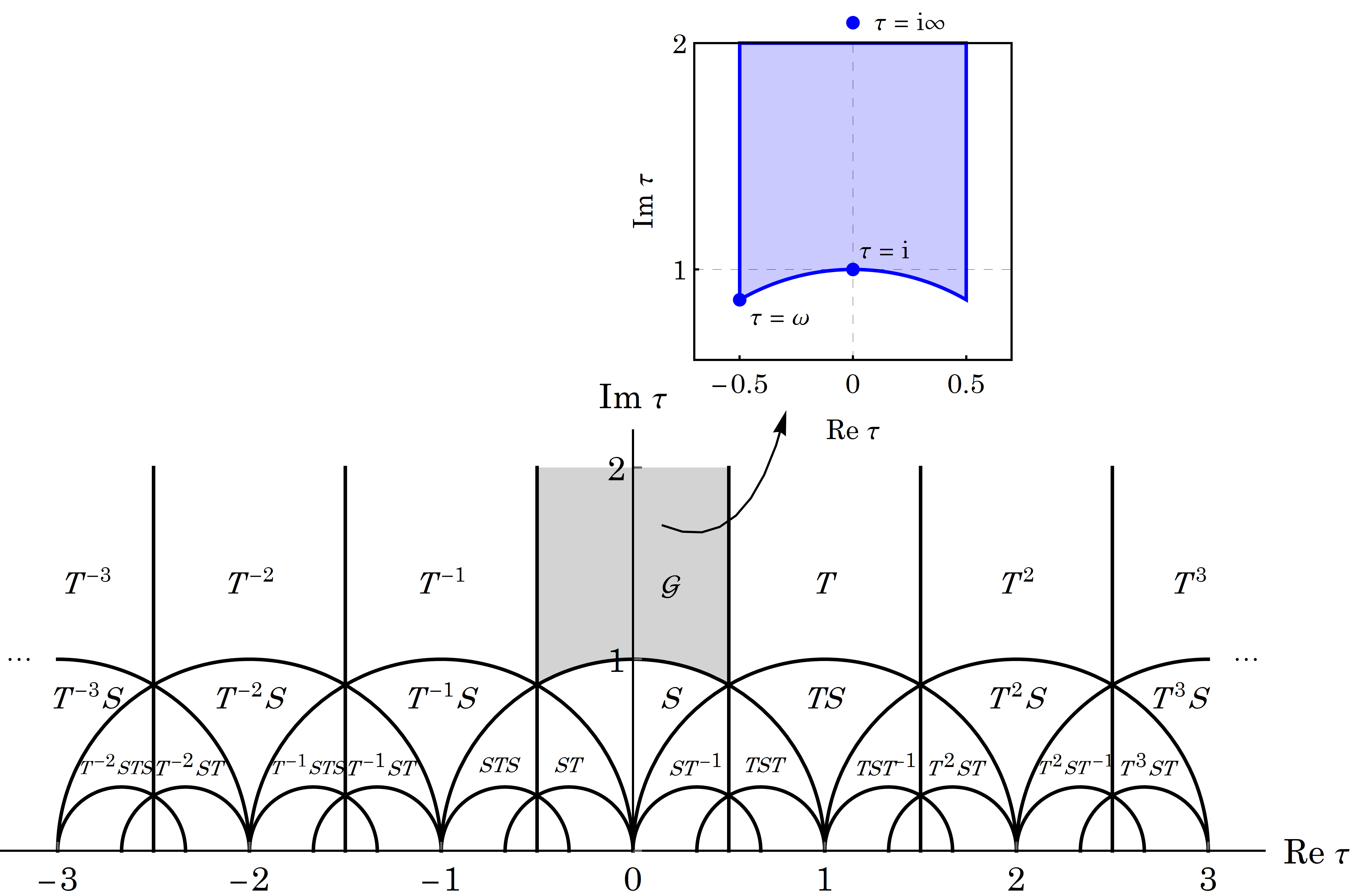
Figure 1: Fundamental domain ${\mathcal{G}}$ of $\overline{\Gamma}$. Acting $\overline{\Gamma}$ on $\mathcal{G}$ generates the entire upper-half complex plane with ${\rm Im}\,\tau>0$. Three fixed points $\tau={\rm i}$, $\omega$ and ${\rm i}\infty$ in $\mathcal{G}$ are labelled by blue dots.

To start with, we briefly review some basic knowledge about modular symmetries in the single- and multiple-modulus framework, as well as the fixed points of moduli. The modular group $\overline{\Gamma}$ is isomorphic to ${\rm PSL}(2,\mathbb{Z})$ defined as Feruglio:2017spp

$$\overline{\Gamma}\equiv\left\{\left(\begin{matrix}a&&b\\ c&&d\end{matrix}\right)/(\pm{\bf I})\;\bigg{|}\;a,b,c,d\in\mathbb{Z}\;,~{}ad-bc=1\right\}\;,$$ (1)

where ${\bf I}$ is a two-dimensional unitary matrix. Under the modular group, the modulus $\tau$ and chiral supermultiplets $\chi^{(I)}$ transform as

$$\gamma:\tau\rightarrow\dfrac{a\tau+b}{c\tau+d}\;,\quad\chi^{(I)}\rightarrow(c\tau+d)^{-k_{I}}\rho_{I}(\gamma)\chi^{(I)}\;,$$ (2)

with $\gamma$ being an element of $\overline{\Gamma}$, $k_{I}$ denoting the weight of the chiral supermultiplet and $\rho_{I}(\gamma)$ representing the unitary representation matrix of $\gamma$. There are two generators $S$ and $T$ in $\overline{\Gamma}$ satisfying $S^{2}=(ST)^{3}={\bf I}$, the matrix representations of which can be written as

$$S=\left(\begin{matrix}0&&1\\ -1&&0\end{matrix}\right)\;,\quad T=\left(\begin{matrix}1&&1\\ 0&&1\end{matrix}\right)\;.$$ (3)

If we act all the elements $\gamma\in\overline{\Gamma}$ on a given point $\tau$ in the upper-half complex plane $\mathbb{C}_{+}=\{\tau\in\mathbb{C}:{\rm Im}\,\tau>0\}$, we will obtain an orbit of $\tau$. Then one can always find a minimal connected set $\mathcal{G}$, where all the orbits intersect the interior of $\mathcal{G}$ in one and only one point. The set $\mathcal{G}$ is called the fundamental domain of $\overline{\Gamma}$ defined as

$${\cal G}=\left\{\tau\in\mathbb{C}_{+}:-\frac{1}{2}\leq{\rm Re}\,\tau<\frac{1}{2},\;|\tau|>1\right\}\;\cup\left\{\tau\in\mathbb{C}_{+}:-\frac{1}{2}\leq{\rm Re}\,\tau\leq 0,\;|\tau|=1\right\}.$$ (4)

Acting $\gamma\in\overline{\Gamma}$ on $\mathcal{G}$ will generate another fundamental domain, as shown in Fig. 1.

The modular form $f(\tau)$ is a holomorphic function of $\tau$ transforming under the modular group as

$$f\left(\gamma\tau\right)=(c\tau+d)^{k}f(\tau)\;,\quad\gamma\in\Gamma(N)\;,$$ (5)

where the level $N$ and weight $k$ are respectively positive and even integers, and $\Gamma(N)$ denote the principle congruence subgroups of $\overline{\Gamma}$. For a given $N$, the modular forms can always be decomposed into several multiplets $Y^{(k)}_{\bf r}=(f_{1}(\tau),f_{2}(\tau),\cdots)^{\rm T}$ that transform as irreducible unitary representations of the quotient subgroups $\Gamma_{N}=\overline{\Gamma}/\Gamma(N)$, namely,

$$Y^{(k)}_{\bf r}(\gamma\tau)=(c\tau+d)^{k}\rho_{\bf r}(\gamma)Y^{(k)}_{\bf r}(\tau)\;,\quad\gamma\in\Gamma_{N}\;,$$ (6)

where $\rho_{\bf r}(\gamma)$ denotes the representation matrice of $\Gamma_{N}$. $\Gamma_{N}$ are usually called the finite modular groups, which are isomorphic to non-Abelian discrete groups, e.g., $\Gamma_{3}\simeq A_{4}$, $\Gamma_{4}\simeq S_{4}$ and $\Gamma_{5}\simeq A_{5}$.

Now consider the modular-invariant supersymmetric theories. The invariance of the action ${\cal S}$ under the modular transformations requires that the Kähler potential $K(\tau,\overline{\tau},\chi,\overline{\chi})$ remains unchanged up to a Kähler transformation ${\cal K}(\tau,\overline{\tau},\chi,\overline{\chi})\rightarrow{\cal K}(\tau,\overline{\tau},\chi,\overline{\chi})+u(\tau,\chi)+u(\overline{\tau},\overline{\chi})$ [$u(\tau,\chi)$ itself is invariant under the modular transformation], and the superpotential ${\cal W}(\tau,\chi)$ should exactly keep invariant. For the Kähler potential, the minimal form subject to the Kähler transformation is

$${\cal K}(\tau,\bar{\tau},\chi,\bar{\chi})=-h\log(-{\rm i}\tau+{\rm i}\bar{\tau})+\sum_{I}\frac{\left|\chi^{(I)}\right|^{2}}{(-{\rm i}\tau+{\rm i}\bar{\tau})^{k_{I}}}\;,$$

where $h$ is a positive constant. The superpotential ${\cal W}(\tau,\chi)$ can be generally written as

$${\cal W}(\tau,\chi)=\sum_{p}\sum_{\{I_{1},\dots,I_{p}\}}\left(Y_{I_{1}\dots I_{p}}(\tau)\chi^{(I_{1})}\cdots\chi^{(I_{p})}\right)_{\bf 1}\;.$$ (7)

In order for ${\cal W}(\tau,\chi)$ to be invariant under the modular transformation, the Yukawa couplings $Y_{I_{1}\dots I_{p}}$ should take the modular forms

$$Y_{I_{1}\dots I_{p}}(\gamma\tau)=(c\tau+d)^{k_{Y}}\rho_{Y}(\gamma)Y_{I_{1}\dots I_{p}}(\tau)\;,\quad\gamma\in\Gamma_{N}\;,$$ (8)

where $\rho_{Y}$ denotes the representation matrix and $k_{Y}$ is the weight of $Y_{I_{1}\dots I_{p}}(\tau)$. Note that $k_{Y}=k_{I_{1}}+\cdots+k_{I_{p}}$ and $\rho_{Y}\otimes\rho_{I_{1}}\otimes\cdots\otimes\rho_{I_{p}}\ni{\bf 1}$ should be satisfied.

The modular symmetry can be extended to the framework of multiple moduli deMedeirosVarzielas:2019cyj . Supposing there are a series of modular groups $\overline{\Gamma}^{1},\overline{\Gamma}^{2},\dots,\overline{\Gamma}^{M}$ associated with different moduli $\tau_{1},\tau_{2},\dots,\tau_{M}$, the modular transformation of each modulus field would be

$$\gamma_{i}:\tau_{i}\to\gamma_{i}\tau_{i}=\frac{a_{i}\tau_{i}+b_{i}}{c_{i}\tau_{i}+d_{i}}\;.$$ (9)

Similar to the single-modulus case, we can obtain a set of finite modular groups $\Gamma^{i}_{N_{i}}=\overline{\Gamma}^{i}/\Gamma^{i}(N_{i})$. The chiral superfield $\chi^{(I)}$ then transforms under the modular group $\Gamma^{1}_{N_{1}}\times\Gamma^{2}_{N_{2}}\times\cdots\times\Gamma_{N_{M}}^{M}$ as

$$\chi^{(I)}(\tau_{1},\dots,\tau_{M}) \to \chi^{(I)}(\gamma_{1}\tau_{1},\dots,\gamma_{M}\tau_{M})$$ (10)

$$= \prod_{i=1,\dots,M}(c_{i}\tau_{i}+d_{i})^{-k_{I,i}}\bigotimes_{i=1,\dots,M}\rho_{I,i}(\gamma_{i})\chi^{(I)}(\tau_{1},\tau_{2},\dots,\tau_{M})\;,$$

where we label the elements in $\Gamma_{N_{i}}^{i}$ as $\gamma_{i}$. In addition, $k_{I,i}$ and $\rho_{I,i}$ are respectively the weights of $\chi^{(I)}$ and the corresponding representation matrices in $\Gamma_{N_{i}}^{i}$, and $\bigotimes$ represents the outer product of the representation matrices $\rho_{I,1}$, $\rho_{I,2}$, $\dots$, $\rho_{I,M}$.

Correspondingly, the Kähler potential can be rewritten as

$${\mathcal{K}}(\tau_{1},\dots,\tau_{M},\overline{\tau}_{1},\dots,\overline{\tau}_{M},\chi,\overline{\chi}) = -\sum_{i=1,...,M}h_{i}\log(-{\rm i}\tau_{i}+{\rm i}\overline{\tau}_{i})$$ (11)

$$+ \sum_{I}\,\frac{\left|\chi^{(I)}\right|^{2}}{\displaystyle\prod_{i=1,...,M}(-{\rm i}\tau_{i}+{\rm i}\overline{\tau}_{i})^{k_{I,i}}}\;.$$

The superpotential ${\cal W}(\tau_{1},\dots,\tau_{M},\chi)$ becomes a modular-invariant function of all the moduli fields as well as the superfields, which takes the form

$${\cal W}(\tau_{1},\dots,\tau_{M},\chi)=\sum_{p}\sum_{\{I_{1},\dots,I_{p}\}}\left(Y_{I_{1},\dots,I_{p}}\chi^{(I_{1})}\cdots\chi^{(I_{p})}\right)_{\mathbf{1}}\;,$$ (12)

Under the modular group, the modular forms $Y_{I_{1},...,I_{p}}$ transform as

$$Y_{I_{1},\dots,I_{p}}(\gamma_{1}\tau_{1},\dots,\gamma_{M}\tau_{M})$$

$$\hskip 34.14322pt=\prod_{i=1,\dots,M}(c_{i}\tau_{i}+d_{i})^{k_{Y,i}}\bigotimes_{i=1,\dots,M}\rho_{Y,i}(\gamma_{i})Y_{I_{1},\dots,I_{p}}(\tau_{1},\dots,\tau_{M})\;.$$ (13)

Since the modular symmetries associated with different moduli are independent of each other, one modulus field obtaining its VEV will not affect the others. Once all the moduli acquire their individual VEVs, the entire modular symmetry will be spontaneously broken down. However, there are some fixed points of $\tau$, where the modular symmetry is only partially broken and we are left with residual symmetries Novichkov:2018ovf . There are three different fixed points in the fundamental domain $\cal{G}$ (cf. Fig. 1), namely,

• $\tau_{\rm C}={\rm i}$, which is invariant under $S$ and preserve a $Z^{S}_{2}$ symmetry;

• $\tau_{\rm L}=-1/2+{\rm i}\sqrt{3}/2$, which is invariant under $ST$ and preserve a $Z^{ST}_{3}$ symmetry;

• $\tau_{\rm T}={\rm i}\infty$, which is invariant under $T$ and preserve a $Z^{T}_{2}$ symmetry.

It is very interesting to investigate whether these special points which are fixed by residual symmetries also have dynamical origins. This is exactly the main motivation for our work.

2.2 $\mathcal{N}=1$ supergravity theory

We consider the ${\cal N}=1$ supergravity theory in the Abelian heterotic orbifolds, which should generally include the dilaton, the Kähler moduli, the complex structure moduli, gauge fields and twisted and untwisted matter fields. Here we focus on a simple scenario where only the Kähler moduli $\tau_{i}$ and the dilaton field $S$ are relevant for the scalar potential.

Let us first consider the case of one Kähler modulus $\tau$ plus one dilaton field $S$. In the framework of supergravity theory, supersymmetry should be regarded as a local symmetry. In this case, the Kähler potential and the superpotential are dependent on each other via the following modular-invariant Kähler function

$$G(\tau,\overline{\tau},S,\overline{S})={\cal K}(\tau,\overline{\tau},S,\overline{S})+\log\left|{\cal W}(\tau,S)\right|^{2}\;.$$ (14)

Assuming the Kähler potential of $\tau$ to be the minimal form, ${\cal K}(\tau,\overline{\tau},S,\overline{S})$ can be essentially expressed as

$${\cal K}(\tau,\overline{\tau},S,\overline{S})=K(S,\overline{S})-3\log(2\,{\rm Im}\,\tau)\;,$$ (15)

with $K(S,\overline{S})$ representing the Kähler potential for the dilaton. At tree level, we have a simple relation $K(S,\overline{S})\propto-{\rm ln}\,(S+\overline{S})$, which is related to the 4d universal gauge coupling via $g^{2}_{4}/2=1/\langle S+\overline{S}\rangle$ once the dilaton gets its VEV. However, if non-perturbative effects such as the Shenker-like effects are included Shenker:1990 , additional corrections $\delta K(S,\overline{S})$ could be added into $K(S,\overline{S})$. We will see later that such effects play a crucial role in generating dS vacua. On the other hand, it is straightforward to check that ${\rm Im}\,\tau\to|c\tau+d|^{-2}{\rm Im}\,\tau$ under the modular transformation, hence $e^{\cal K}$ should possess a weight of six. The modular invariance of $G(\tau,\overline{\tau})$ implies that the transformation of ${\cal K}(\tau,\overline{\tau},S,\overline{S})$ under the modular group is compensated by that of ${\cal W}(\tau)$. As a result, under the modular group ${\cal W}(\tau)$ should transform as

$${\cal W}(\tau)\to(c\tau+d)^{-3}{\cal W}(\tau)\;,$$ (16)

indicating the superpotential possesses a weight of $-3$ under the modular transformation. In the next subsection, we will show that the superpotential satisfying Eq. (16) can be induced by a non-perturbative effect—gaugino condensation.

Once the Kähler potential and superpotential are known, we can construct the scalar potential $V$ as Cremmer:1982en

$$V=e^{\cal K}\left({\cal K}^{i\bar{j}}D_{i}{\cal W}D_{\bar{j}}{\cal W}^{*}-3|{\cal W}|^{2}\right)\;,$$ (17)

where $D_{i}=\partial_{i}+(\partial_{i}{\cal K})$ with $\partial_{i}$ being the first derivatives with respect to the Kähler moduli (which is simply $\partial/\partial\tau$ in the single-modulus case) together with the dilaton, and ${\cal K}^{i\overline{j}}$ is the inverse of the Kähler metric ${\cal K}_{i\overline{j}}=\partial_{i}\partial_{\overline{j}}{\cal K}$. The scalar potential given in Eq. (17) is modular-invariant, which is proved in appendix A.

2.3 Gaugino condensation

In the heterotic string constructions, gaugino condensation is a simple example that can lead to the spontaneous breakdown of supersymmetry. A gauge group $G_{a}$ undergoing gaugino condensation will give rise to a non-perturbative superpotential of the form Dine:1985rz ; Nilles:1982ik ; Ferrara:1982qs

$${\cal W}\sim e^{-f_{a}/b_{a}}\;,$$ (18)

where $f_{a}$ is the gauge kinetic function and $b_{a}$ is the beta function of the group $G_{a}$. At the tree level, the gauge kinetic function simply takes the form $f_{a}=k_{a}S$ with $k_{a}$ being the level of the Kac-Moody algebra of $G_{a}$, which is apparently moduli-independent. However, if the orbifolds of our interest arise in ${\cal N}=2$ subsectors, threshold corrections to the gauge kinetic functions induced by integrating out heavy string states should be taken into consideration Giddings:2001yu ; Gukov:1999ya ; Curio:2000sc ; Ashok:2003gk ; Denef:2004cf . In the single-modulus case, the modified $f_{a}$ can be written as

$$f_{a}=k_{a}S+b_{a}{\rm ln}\,\eta^{6}(\tau)+\cdots\;,$$ (19)

where $\eta(\tau)$ is the Dedekind $\eta$ function (See appendix B for the definition). The modulus-dependent term $b_{a}{\rm ln}\,\eta^{6}(\tau)$ indicates that ${\cal W}$ indeed transforms under the modular group with a weight of $-3$, and the dots denote additional contributions to threshold corrections which are also modulus-dependent but keep invariant under the modular transformation. Apart from the threshold corrections, one-loop anomaly cancellation could also lead to significant modifications to $f_{a}$ Derendinger:1991hq ; Lust:1991yi ; LopesCardoso:1991ifk ; LopesCardoso:1992yd , which however can be absorbed into $S$ by redefining the dilaton field Kaplunovsky:1995jw . Substituting Eq. (19) into Eq. (18), we arrive at the following parameterised form of ${\cal W}$

$${\cal W}(\tau,S)=\frac{\Omega(S)H(\tau)}{\eta^{6}(\tau)}\;,$$ (20)

where $\Omega(S)$ denotes a function of the dilaton field $S$, and $H(\tau)$ is a dimensionless modular-invariant function. We can further require $H(\tau)$ to be a rational function to avoid any singularity in the fundamental domain, thus the most general form of $H(\tau)$ should be Cvetic:1991qm

$$H(\tau)=(j(\tau)-1728)^{m/2}j(\tau)^{n/3}{\cal P}(j(\tau))\;,$$ (21)

with $j(\tau)$ being the Klein $j$ function which is invariant under the modular transformation defined in appendix B, $m$ and $n$ being non-negative integers and ${\cal P}$ denoting a polynomial with respect to $j(\tau)$. In the following, we take ${\cal P}=1$ for simplicity. It is interesting to mention that $j(\omega)=0$ and $j({\rm i})=12^{3}=1728$ are satisfied at the two fixed points $\tau=\omega$ and ${\rm i}$, respectively.

Once we substitute the Kähler potential in Eq. (15) and the superpotential in Eq. (20) into Eq. (17), the single-modulus scalar potential can be immediately expressed as

$$V(\tau,\overline{\tau},S,\overline{S})=\mathcal{C}(\tau,\overline{\tau},S,\overline{S})\left[\mathcal{M}(\tau,\overline{\tau})+\left(\mathcal{A}(S,\overline{S})-3\right)|H(\tau)|^{2}\right]\;,$$ (22)

with

$$\begin{split}\mathcal{C}(\tau,\overline{\tau},S,\overline{S})&=\dfrac{e^{K(S,\overline{S})}|\Omega(S)|^{2}}{(2\,{\rm Im}\,\tau)^{3}|\eta(\tau)|^{12}}\;,\\ \mathcal{M}(\tau,\overline{\tau})&=\frac{(2\,{\rm Im}\,\tau)^{2}}{3}\left|{\rm i}H^{\prime}(\tau)+\frac{H(\tau)}{2\pi}\widehat{G}_{2}(\tau,\overline{\tau})\right|^{2}\;,\\ \mathcal{A}(S,\overline{S})&=\frac{|\Omega_{S}+K_{S}\Omega|^{2}}{K_{S\overline{S}}|\Omega|^{2}}\;,\end{split}$$ (23)

where the subscripts $S$ and $\overline{S}$ represent the first derivatives with respect to $S$ and $\overline{S}$, respectively, and $K^{S\overline{S}}=(K_{S\overline{S}})^{-1}$. Moreover, $\widehat{G}_{2}$ is the non-holomorphic Eisenstein function of weight two defined as

$$\widehat{G}_{2}(\tau,\overline{\tau})=G_{2}(\tau)-\frac{\pi}{{\rm Im}\,\tau}\;,$$ (24)

where the Eisenstein series $G_{2}$ is a holomorphic counterpart of $\widehat{G}_{2}(\tau,\overline{\tau})$, and can be related to the Dedekind $\eta$ function via

$$\frac{\eta^{\prime}(\tau)}{\eta(\tau)}=\frac{\rm i}{4\pi}G_{2}(\tau)\;.$$ (25)

3 Modulus stabilisation

3.1 Minimising the single-modulus scalar potential

Before going into the details of minimising the scalar potential, we can first gain some general insights without specifying the form of the scalar potential. One salient feature of the scalar potential is that it diverges in the limit ${\rm Im}\,\tau\to\infty$. Hence the fixed point $\tau\to{\rm i}\infty$ seems not to be the vacuum. The finite fixed points, however, are able to be the minima of the scalar potential. In fact, since $V$ is a zero-weight modular form, $\partial V/\partial\tau$ must be a modular form with weight two (See appendix A for proof). Then if we consider the modular transformation of $\partial V/\partial\tau$ under the generator $S$ at $\tau={\rm i}$, we will arrive at

$$\left.(\partial V/\partial\tau)\right|_{\tau={\rm i}}=(-{\rm i})^{2}\left.(\partial V/\partial\tau)\right|_{\tau={\rm i}}=-\left.(\partial V/\partial\tau)\right|_{\tau={\rm i}}\;.$$ (26)

Similarly, if we consider the modular transformation of $\partial V/\partial\tau$ under the generator $ST$ at $\tau=\omega$, we will obtain

$$\left.(\partial V/\partial\tau)\right|_{\tau=\omega}=(-\omega-1)^{2}\left.(\partial V/\partial\tau)\right|_{\tau=\omega}=\omega\left.(\partial V/\partial\tau)\right|_{\tau=\omega}\;.$$ (27)

Eqs. (26) and (27) tell us $\partial V/\partial\tau$ has to be zero at $\tau={\rm i}$ and $\omega$. Therefore the finite fixed points should be the extrema of the scalar potential in the Kähler moduli space. However, identifying whether they are exactly the minima requires an in-depth analysis of certain scalar potentials.

Another important point is that the dilaton sector also affects modulus stabilisation, namely, the scalar potential should satisfy $\partial V/\partial S=0$ at the minima. Hence we arrive at

$$\frac{\partial V}{\partial S}=\dfrac{e^{K}}{(2\,{\rm Im}\,\tau)^{3}|\eta(\tau)|^{12}}(\Omega_{S}+K_{S}\Omega){\mathcal{Q}}=0\;,$$ (28)

where

$${\mathcal{Q}}= e^{-2{\rm i}\sigma}|H|^{2}\left[(\Omega_{S}+K_{S}\Omega)\left(\frac{K_{S}}{K_{S\overline{S}}}-\frac{K_{SS\overline{S}}}{K^{2}_{S\overline{S}}}\right)+\frac{\Omega_{S\overline{S}}}{K_{S\overline{S}}}+\frac{\Omega K_{SS}}{K_{S\overline{S}}}+\frac{\Omega_{S}K_{S}}{K_{S\overline{S}}}\right]$$ (29)

$$+\overline{\Omega}\left(\mathcal{M}-2|H|^{2}\right)\;,$$ (30)

with $\sigma$ being the phase angle of $\Omega_{S}+K_{S}\Omega$. Then we can immediately gain the following two possibilities of the necessary conditions for $S$ to be stabilised

$$\begin{split}{\it Condition~{}A:}\quad&\Omega_{S}+K_{S}\Omega=0\;;\\ {\it Condition~{}B:}\quad&\Omega_{S}+K_{S}\Omega\neq 0\;,\quad{\cal Q}=0\;.\end{split}$$ (31)

Indeed, Condition A corresponds to the case where ${\mathcal{A}}(S,\overline{S})$ is vanishing, i.e., the scalar potential can be written as a factorised form of the dilaton and Kähler moduli sector. This scenario has been widely studied in the previous literature Font:1990nt ; Cvetic:1991qm ; Gonzalo:2018guu ; Novichkov:2022wvg . In Refs. Cvetic:1991qm ; Gonzalo:2018guu , assuming ${\mathcal{A}}(S,\overline{S})=0$, the authors analyse different scalar potentials by varying the indices $m$ and $n$ in Eq. (21). They have numerically searched the minima of the scalar potentials and concluded that the vacua should appear either on the lower boundary of the fundamental domain or on the imaginary axis of $\tau$. The authors in Ref. Novichkov:2022wvg find a special case where $m\neq 0$ and $n=0$ can lead to global minima very close to but not precisely at the fixed point $\tau=\omega$. In summary, there are four different types of vacua depending on the choices of $m$ and $n$ if Condition A is satisfied:

• $m=0$ and $n=0$: The vacuum $\langle\tau\rangle=1.235{\rm i}$;

• $m\neq 0$ and $n=0$: The vacuum $\langle\tau\rangle={\rm i}$;

• $m=0$ and $n\neq 0$: The vacua are close to but not precisely at $\tau=\omega$;

• $m\neq 0$ and $n\neq 0$: The vacua are located at the lower boundary of the fundamental domain.

It is worth mentioning that all the above vacua will give rise to negative values of the scalar potential, i.e., they are actually AdS vacua. In Ref. Leedom:2022zdm , the authors have proved three no-go theorems regarding the dS vacua, indicating Condition A can never lead to dS vacua. On the other hand, even if it is possible for the extrema that satisfy Condition B to be the dS vacua, such vacua may still be unstable in the dilaton sector. In particular, one can prove that if only the tree-level Kähler potential for the dilaton $K(S,\overline{S})\propto-{\rm ln}\,(S+\overline{S})$ is included, $\tau={\rm i}$ and $\omega$ could never be the dS vacua no matter which form $\Omega(S)$ takes Leedom:2022zdm . In order to evade the dS no-go theorems, one should go beyond the minimal Kähler potential of $S$. It is found in Ref. Leedom:2022zdm that non-perturbative Shenker-like effects can result in non-trivial corrections to $K(S,\overline{S})$, rendering the dilaton sector stable at the fixed points $\tau={\rm i}$ and $\omega$. Different from the gaugino condensation which has a generic strength $\delta{\cal L}=e^{-1/g^{2}_{s}}$ with $g_{s}$ being the string coupling constant, Shenker-like effects are inherently stringy effects which lead to modifications of ${\mathcal{O}}(e^{-1/g_{s}})$. In the rest of this paper, we will not concentrate on how to realise specific Shenker-like terms and how they can stabilise the dilaton sector. Instead, we assume the dilaton is stabilised a priori, and explore how the value of ${\cal A}(S,\overline{S})$ in Eq. (22) can influence the modulus stabilisation.

Nonzero ${\cal A}(S,\overline{S})$ can dramatically reshape the scalar potential, and thus shift the vacua. To be specific, the dS vacua may appear precisely at the finite fixed points. In order to make this point clearer, we can calculate the Hessian matrices at the fixed points. Since we have assumed the scalar potential is stabilised in terms of the dilaton $S$ via Shenker-like terms a priori, we only need to calculate the second derivatives of $V$ with respect to $\tau$ and $\overline{\tau}$, and convert the complex variables into real variables $\{s,t\}$ (where $s$ and $t$ are the real and imaginary parts of $\tau$, respectively) using the following relations

$$\begin{split}\frac{\partial^{2}V}{\partial s^{2}}&=2\frac{\partial^{2}V}{\partial\tau\partial\overline{\tau}}+2\,{\rm Re}\left[\frac{\partial^{2}V}{\partial\tau^{2}}\right]\;,\\ \frac{\partial^{2}V}{\partial t^{2}}&=2\frac{\partial^{2}V}{\partial\tau\partial\overline{\tau}}-2\,{\rm Re}\left[\frac{\partial^{2}V}{\partial\tau^{2}}\right]\;,\\ \frac{\partial^{2}V}{\partial s\partial t}&=-2\,{\rm Im}\left[\frac{\partial^{2}V}{\partial\tau^{2}}\right]\;.\end{split}$$ (32)

In general, the second derivatives of the scalar potential would be very complicated given that $V$ relies on the moduli $\tau$ in a highly non-linear way. However, one can easily check that the first derivatives of ${\cal C}$ and ${\cal M}$ defined in Eq. (23) with respect to $\tau$ vanish at the fixed points $\tau={\rm i}$ and $\omega$, rendering the calculations of the second derivatives at the fixed points much simpler. As a result, we arrive at

$$\begin{split}\frac{\partial^{2}V}{\partial\tau^{2}}&=\frac{\partial^{2}{\mathcal{C}}}{\partial\tau^{2}}\left[{\mathcal{M}}+(\mathcal{A}-3)|H|^{2}\right]+{\mathcal{C}}\left[\frac{\partial^{2}{\mathcal{M}}}{\partial\tau^{2}}+(\mathcal{A}-3)H^{*}\frac{\partial^{2}H}{\partial\tau^{2}}\right]\;,\\ \frac{\partial^{2}V}{\partial\tau\partial\overline{\tau}}&=\frac{\partial^{2}{\mathcal{C}}}{\partial\tau\partial\overline{\tau}}[{\mathcal{M}}+(\mathcal{A}-3)|H|^{2}]+{\mathcal{C}}\left[\frac{\partial^{2}{\mathcal{M}}}{\partial\tau\partial\overline{\tau}}+(\mathcal{A}-3)\left|\frac{\partial H}{\partial\tau}\right|^{2}\right]\;,\end{split}$$ (33)

with

$$\begin{split}\frac{\partial^{2}{\mathcal{C}}}{\partial\tau^{2}}&=-{\rm i}{\mathcal{C}}\frac{\partial}{\partial\tau}\frac{\widehat{G}_{2}(\tau,\overline{\tau})}{6\pi}\;,\\ \frac{\partial^{2}{\mathcal{C}}}{\partial\tau\partial\overline{\tau}}&={\rm i}{\mathcal{C}}\frac{\partial}{\partial\tau}\frac{[\widehat{G}_{2}(\tau,\overline{\tau})]^{*}}{6\pi}\;,\\ \frac{\partial^{2}{\mathcal{M}}}{\partial\tau^{2}}&=\frac{(2\,{\rm Im}\,\tau)^{2}}{3}\left[{\rm i}\frac{\partial^{2}H(\tau)}{\partial\tau^{2}}+\frac{H(\tau)}{2\pi}\frac{\partial\widehat{G}_{2}(\tau,\overline{\tau})}{\partial\tau}\right]\frac{H^{*}(\tau)}{\pi}\frac{\partial\widehat{G}^{*}_{2}(\tau,\overline{\tau})}{\partial\tau}\;,\\ \frac{\partial^{2}{\mathcal{M}}}{\partial\tau\partial\overline{\tau}}&=\frac{(2\,{\rm Im}\,\tau)^{2}}{3}\left[\left|{\rm i}\frac{\partial^{2}H(\tau)}{\partial\tau^{2}}+\frac{H(\tau)}{2\pi}\frac{\partial\widehat{G}_{2}(\tau,\overline{\tau})}{\partial\tau}\right|^{2}+\left|\frac{H(\tau)}{2\pi}\frac{\partial{\widehat{G}_{2}(\tau,\overline{\tau})}}{\partial\overline{\tau}}\right|^{2}\right]\;,\end{split}$$ (34)

where all the derivatives above are calculated at the $\tau={\rm i}$ or $\omega$. One can check that the imaginary parts of $\partial^{2}V/\partial\tau^{2}$ are zero at the finite fixed points. Hence we arrive at the $2\times 2$ diagonal Hessian matrices

$${\mathbf{H}}=\left(\begin{matrix}\dfrac{\partial^{2}V}{\partial s^{2}}&0\\ 0&\dfrac{\partial^{2}V}{\partial t^{2}}\\ \end{matrix}\right)\;.$$ (35)

In order for finite fixed points to be the minima of the scalar potential, we should require both $\partial^{2}V/\partial s^{2}$ and $\partial^{2}V/\partial t^{2}$ in Eq. (35) to be positive at the fixed points. For example, if we set $(m,n)=(0,0)$, the conditions for $\tau={\rm i}$ and $\omega$ to be the minima are respectively given by

$$\begin{split}\tau={\rm i}:&\quad 3.596-\mathcal{A}>0\;,\quad\mathcal{A}-0.4036>0\;;\\ \tau=\omega:&\quad\mathcal{A}-2>0\;.\end{split}$$ (36)

Notice that $\mathcal{A}>3$ should also be satisfied if we require dS vacua, which can be directly obtained from Eq. (22) given that ${\mathcal{M}}=0$ and $|H|\geq 0$ at the fixed points. Hence $\tau={\rm i}$ could be the dS vacuum if $3<{\cal A}(S,\overline{S})<3.5964$ is satisfied, while $\tau=\omega$ can always be the dS vacuum as long as ${\cal A}(S,\overline{S})>3$. A detailed analysis of minimising the one-modulus scalar potential can be found in Ref. Leedom:2022zdm . The main conclusions are collected as follows:

• $m=0$ and $n=0$: $\tau=\omega$ is always the dS vacuum, while $\tau={\rm i}$ can be the dS vacuum if $3<{\cal A}(S,\overline{S})<3.5964$ is satisfied;

• $m>1$, $n=0$: $\tau=\omega$ is always a dS vacuum if ${\cal A}(S,\overline{S})>3$, and $\tau={\rm i}$ is a Minkowski vacuum;

• $m=0$, $n>1$: $\tau={\rm i}$ is a dS vacuum within a window of ${\cal A}(S,\overline{S})$ which increases with $n$, and $\tau=\omega$ is a Minkowski vacuum.

• $m=1$ or $n=1$: $\tau={\rm i}$ or $\tau=\omega$ could be the minimum in terms of the Kähler modulus, but it is actually unstable in the dilaton sector;

• $m>1$, $n>1$: Both $\tau={\rm i}$ and $\tau=\omega$ are Minkowski vacua when ${\cal A}(S,\overline{S})>3$.

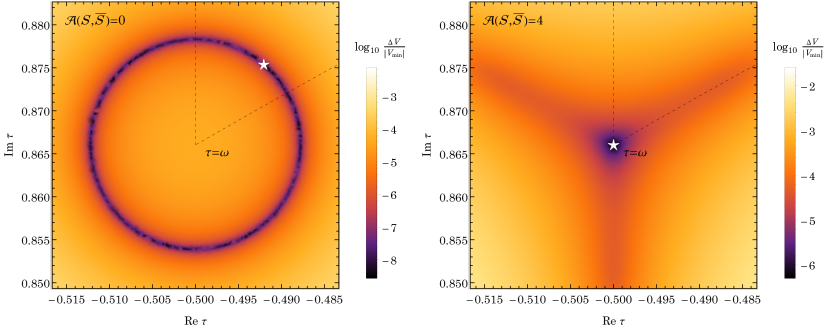
Figure 2: Density plots of the distribution of ${\rm log}_{10}(\Delta V/|V_{\rm min}|)$ with $\Delta V=V-V_{\rm min}$ in the vicinity of $\tau=\omega$. We take $m=2$ and $n=0$ for instance. In the left panel, we choose ${\cal A}(S,\overline{S})=0$, while ${\cal A}(S,\overline{S})$ is fixed to be four in the right panel. We use white stars to label the vacua. The dashed lines correspond to the boundaries of the fundamental domain.

As can be seen above, the inclusion of dilaton effects will not only uplift the vacua to dS vacua, but also shift the VEVs of $\tau$ towards the fixed points. For illustration, we consider a specific case with $m=2$ and $n=0$. In Fig. 2, we exhibit the distribution of ${\rm log}_{10}(\Delta V/|V_{\rm min}|)$ with $\Delta V$ defined as the difference between $V$ and its minimal value $V_{\rm min}$ in the vicinity of $\tau=\omega$ under the assumptions ${\cal A}(S,\overline{S})=0$ and ${\cal A}(S,\overline{S})=4$, respectively. In the case where ${\cal A}(S,\overline{S})=0$, the fixed point $\tau=\omega$ turns out to be a local maximum, and the global AdS vacuum appears at $\tau=-0.492+0.875{\rm i}$ with $V_{\rm min}=-2.48\times 10^{7}$, which is consistent with the result in Ref. Novichkov:2022wvg . However, if ${\cal A}(S,\overline{S})>3$, e.g., ${\cal A}(S,\overline{S})=4$, we obtain a vacuum precisely at $\tau=\omega$, where the value of $V$ are found to be $V_{\rm min}=8.29\times 10^{6}$, indicating $\tau=\omega$ is indeed a dS vacuum.

One may wonder whether it is possible to obtain dS vacua at the points which are close to but not precisely at the fixed points. $\tau=\omega$ is always the dS/Minkowski minimum of the scalar potential as long as ${\cal A}(S,\overline{S})>3$, so it is natural to expect that there would be no chance to find another dS vacuum close to $\tau=\omega$. As for the other fixed point $\tau={\rm i}$, there are indeed some ranges of ${\cal A}(S,\overline{S})$, where $\tau={\rm i}$ is not the vacuum but the scalar potential takes a positive value, e.g., ${\cal A}(S,\overline{S})>3.5964$ when $(m,n)=(0,0)$. In Fig. 3, we exhibit the distribution of $\log_{10}(\Delta V/|V_{\rm min}|)$ in the fundamental domain choosing $(m,n)=(0,0)$ and ${\cal A}(S,\overline{S})=4$. One can observe that $\tau={\rm i}$ becomes a saddle point and no vacuum appears around $\tau={\rm i}$, which can also be identified given that $(\partial^{2}V/\partial s^{2}{})|_{\tau={\rm i}}<0$ and $(\partial^{2}V/\partial t^{2})|_{\tau={\rm i}}>0$. Therefore, it is difficult to realise a dS vacuum close to the fixed points even if non-perturbative effects in the dilaton sector are taken into consideration.

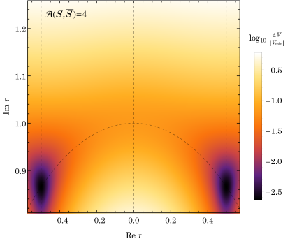
Figure 3: Density plots of the distribution of ${\rm log}_{10}(\Delta V/|V_{\rm min}|)$ in the fundamental domain with $m=0$ and $n=0$, where we choose ${\cal A}(S,\overline{S})=4$.

3.2 Modulus stabilisation in the three-modulus framework

Since the compactification of 10d heterotic string theory will generally lead to three moduli, associated with three 2d tori, we should extend the single modulus stabilisation into this more complete scenario, and explore how the non-perturbative effects can give a dynamical explanation of the VEVs of moduli with multiple modular symmetries.

In the three-modulus case, the modular-invariant function $H(\tau)$ in the superpotential should be replaced by a more general form ${\cal H}(\tau_{1},\tau_{2},\tau_{3})$ with

$$\mathcal{H}(\tau_{1},\tau_{2},\tau_{3})=\sum_{\begin{subarray}{c}m_{1},m_{2},m_{3}\\ n_{1},n_{2},n_{3}\end{subarray}}H^{(m_{1},n_{1})}(\tau_{1})H^{(m_{2},n_{2})}(\tau_{2})H^{(m_{3},n_{3})}(\tau_{3})\;,$$ (37)

where $H^{(m_{i},n_{i})}=(j(\tau)-1728)^{m_{i}/2}j(\tau)^{n_{i}/3}$ for $i=1,2,3$. One may notice that the simplest ${\cal H}(\tau_{1},\tau_{2},\tau_{3})$ should be a factorised form $H^{(m_{1},n_{1})}(\tau_{1})H^{(m_{2},n_{2})}(\tau_{2})H^{(m_{3},n_{3})}(\tau_{3})$, which, however would become zero as long as one $H^{(m_{i},n_{i})}(\tau_{i})$ is vanishing. Consequently, this scenario will essentially lead to Minkowski vacua at the fixed points. Instead, we consider ${\cal H}(\tau_{1},\tau_{2},\tau_{3})$ as the summation of three different $H^{(m_{i},n_{i})}(\tau_{i})$, namely,

$${\cal H}(\tau_{1},\tau_{2},\tau_{3})=H^{(m_{1},n_{1})}(\tau_{1})+H^{(m_{2},n_{2})}(\tau_{2})+H^{(m_{3},n_{3})}(\tau_{3})\;.$$ (38)

Then ${\cal H}(\tau_{1},\tau_{2},\tau_{3})$ would be nonzero as long as at least one of $H^{(m_{i},n_{i})}(\tau_{i})$ is non-vanishing, which makes it more likely to realise the dS vacua. As a result, the Kähler potential and superpotential can be respectively rewritten as

$${\cal K}(\tau_{i},\overline{\tau}_{i},S,\overline{S}) = K(S,\overline{S})-\log[(2\,{\rm Im}\,\tau_{1})(2\,{\rm Im}\,\tau_{2})(2\,{\rm Im}\,\tau_{3})]\;,$$ (39)

$${\cal W}(\tau_{i},S) = \frac{\Omega(S)[H^{(m_{1},n_{1})}(\tau_{1})+H^{(m_{2},n_{2})}(\tau_{2})+H^{(m_{3},n_{3})}(\tau_{3})]}{\eta^{2}(\tau_{1})\eta^{2}(\tau_{2})\eta^{2}(\tau_{3})}\;,$$ (40)

where the variables $\tau_{i}$ go through $\{\tau_{1},\tau_{2},\tau_{3}\}$. The scalar potential in this scenario turns out to be

$$V(\tau_{i},\overline{\tau_{i}},S,\overline{S})=\widetilde{\mathcal{C}}(\tau_{i},\overline{\tau_{i}},S,\overline{S})\left\{\widetilde{\mathcal{M}}(\tau_{i},\overline{\tau}_{i})+\left[\mathcal{A}(S,\overline{S})-3\right]|\mathcal{H}(\tau_{i})|^{2}\right\}\;,$$ (41)

with

$$\begin{split}\widetilde{\mathcal{C}}(\tau_{i},\overline{\tau_{i}},S,\overline{S})&=\prod_{i=1}^{3}\dfrac{e^{K(S,\overline{S})}|\Omega(S)|^{2}}{(2\,{\rm Im}\,\tau_{i})|\eta(\tau_{i})|^{4}}\;,\\ \widetilde{\mathcal{M}}(\tau_{i},\overline{\tau}_{i})&=\sum^{3}_{i=1}(2\,{\rm Im}\,\tau_{i})^{2}\left|{\rm i}\frac{\partial H^{(m_{i},n_{i})}(\tau_{i})}{\partial\tau_{i}}+\sum_{j=1}^{3}\frac{H^{(m_{j},n_{j})}(\tau_{j})}{2\pi}\widehat{G}_{2}(\tau_{i},\overline{\tau}_{i})\right|^{2}\;,\end{split}$$ (42)

One can observe that apart from $\tau_{1,2,3}$ and $\mathcal{A}(S,\overline{S})$, there are additional six parameters that can affect the minima of the scalar potential, namely, $m_{1,2,3}$ and $n_{1,2,3}$. In the following, we discuss the minimisation of the scalar potential given in Eq. (41), mainly focusing attention on the finite fixed points ${\rm i}$ and $\omega$. In order to identify whether they are indeed the minima of the potential, we again calculate the Hessian matrices at the fixed points and make them positive-definite. We also thoroughly search the minima of $V$ in the entire fundamental domain for different $m_{1,2,3}$, $n_{1,2,3}$ and $\mathcal{A}(S,\overline{S})$ in a numerical way, which could help us identify when the fixed points can be the deepest vacua, i.e., the global minima of the scalar potential.

The second derivatives of $V$ in terms of Kähler moduli are expressed as

$$\begin{split}\frac{\partial^{2}V}{\partial\tau^{2}_{i}}&=\frac{\partial^{2}\widetilde{\mathcal{C}}}{\partial\tau^{2}_{i}}\left[\widetilde{\mathcal{M}}+(\mathcal{A}-3)|\mathcal{H}|^{2}\right]+\widetilde{\mathcal{C}}\left[\frac{\partial^{2}\widetilde{\mathcal{M}}}{\partial\tau^{2}_{i}}+(\mathcal{A}-3)\mathcal{H}^{*}\frac{\partial^{2}H^{(m_{i},n_{i})}}{\partial\tau^{2}_{i}}\right]\;,\\ \frac{\partial^{2}V}{\partial\tau_{i}\partial\overline{\tau}_{j}}&=\frac{\partial^{2}\widetilde{\mathcal{C}}}{\partial\tau_{i}\partial\overline{\tau}_{j}}[\widetilde{\mathcal{M}}+(\mathcal{A}-3)|\mathcal{H}|^{2}]+\widetilde{\mathcal{C}}\left[\frac{\partial^{2}\widetilde{\mathcal{M}}}{\partial\tau_{i}\partial\overline{\tau}_{j}}+(\mathcal{A}-3)\left|\frac{\partial H^{(m_{i},n_{i})}}{\partial\tau_{i}}\right|^{2}\right]\;,\end{split}$$ (43)

with

$$\frac{\partial^{2}\widetilde{\mathcal{C}}}{\partial\tau_{i}\partial\tau_{j}} =-{\rm i}\delta_{ij}\widetilde{\mathcal{C}}\frac{\partial}{\partial\tau_{i}}\frac{\widehat{G}_{2}(\tau_{i},\overline{\tau}_{i})}{2\pi}\;,$$

$$\frac{\partial^{2}\widetilde{\mathcal{C}}}{\partial\tau_{i}\partial\overline{\tau}_{j}} ={\rm i}\delta_{ij}\widetilde{\mathcal{C}}\frac{\partial}{\partial\tau_{i}}\frac{[\widehat{G}_{2}(\tau_{j},\overline{\tau}_{j})]^{*}}{2\pi}\;,$$

$$\frac{\partial^{2}\widetilde{\mathcal{M}}}{\partial\tau_{i}\partial\tau_{j}} =\delta_{ij}(2\,{\rm Im}\,\tau_{i})^{2}\left[{\rm i}\frac{\partial^{2}H^{(m_{i},n_{i})}(\tau_{i})}{\partial\tau^{2}_{i}}+\frac{\mathcal{H}(\tau_{i})}{2\pi}\frac{\partial\widehat{G}_{2}(\tau_{i},\overline{\tau}_{i})}{\partial\tau_{i}}\right]\frac{\mathcal{H}^{*}(\tau_{i})}{\pi}\frac{\partial\widehat{G}^{*}_{2}(\tau_{i},\overline{\tau}_{i})}{\partial\tau_{i}}\;,$$

$$\frac{\partial^{2}\widetilde{\mathcal{M}}}{\partial\tau_{i}\partial\overline{\tau}_{j}} =\delta_{ij}(2\,{\rm Im}\,\tau_{i})^{2}\left[\left|{\rm i}\frac{\partial^{2}H^{(m_{i},n_{i})}(\tau_{i})}{\partial\tau^{2}_{i}}+\frac{\mathcal{H}(\tau_{i})}{2\pi}\frac{\partial\widehat{G}_{2}(\tau_{i},\overline{\tau}_{i})}{\partial\tau_{i}}\right|^{2}+\left|\frac{\mathcal{H}(\tau_{i})}{2\pi}\frac{\partial{\widehat{G}_{2}(\tau_{i},\overline{\tau}_{i})}}{\partial\overline{\tau}_{i}}\right|^{2}\right]\;,$$ (44)

where all the derivatives above are calculated at the $\tau={\rm i}$ or $\omega$.

According to the choices of $(m_{i},n_{i})$, we have the following three distinct classes:

• Class A—$\bm{(m_{1},n_{1})=(m_{2},n_{2})=(m_{3},n_{3})}.$ This is an exactly symmetric class, where three moduli parameters can be exchanged. It is natural to expect the global minima should appear at $\tau_{1}=\tau_{2}=\tau_{3}$. Then one can find that $\widetilde{\mathcal{C}}(\tau_{i},\overline{\tau}_{i},S,\overline{S})$ and $\widetilde{\mathcal{M}}(\tau_{i},{\overline{\tau}_{i}})$ in Eq. (42) reduce to the single-modulus case, and thus the results for the minima are the same as those obtained in the single-modulus case.

• Class B—$\bm{(m_{1},n_{1})=(m_{2},n_{2})\neq(m_{3},n_{3})}.$ In this case, we can freely exchange $\tau_{1}$ and $\tau_{2}$ without affecting the value of the scalar potential, hence it is effectively a two-modular case, where only two Kähler moduli $\tau_{1}$ (or $\tau_{2}$) and $\tau_{3}$ are independent.

• Class C—$\bm{(m_{1},n_{1})\neq(m_{2},n_{2})\neq(m_{3},n_{3})}.$ This class becomes more complicated since there is no symmetry among the three moduli parameters. In this class we should consider all three moduli as free parameters.

We mainly focus on Class B. In this class, the number of independent real variables is reduced to four, indicating that the Hessian matrices should be four-dimensional. On the other hand, Eq. (44) tells us all the mixed second derivatives in terms of different moduli are vanishing. Moreover, the imaginary parts of $\partial^{2}V/(\partial\tau_{i}\partial\tau_{j})$ are also zero at the finite fixed points. Hence we arrive at the following diagonal Hessian matrices

$${\mathbf{H}}=\left(\begin{matrix}\dfrac{\partial^{2}V}{\partial s^{2}_{1}}&0&0&0\\ 0&\dfrac{\partial^{2}V}{\partial t^{2}_{1}}&0&0\\ 0&0&\dfrac{\partial^{2}V}{\partial s^{2}_{3}}&0\\ 0&0&0&\dfrac{\partial^{2}V}{\partial t^{2}_{3}}\end{matrix}\right)\;.$$ (45)

Therefore, in order for finite fixed points to be the minima of the scalar potential, we should require each element in Eq. (45) to be positive.

Since effectively we have two independent modulus parameters $\tau_{1}$ and $\tau_{3}$, there are twelve kinds of arrangements of the indices $(m_{i},n_{i})$ depending on whether they are zero or not, including

• $(m_{1},n_{1})=(0,0)$, $(m_{3},n_{3})=(0,\underline{n}_{3})$;

• $(m_{1},n_{1})=(0,0)$, $(m_{3},n_{3})=(\underline{m}_{3},0)$;

• $(m_{1},n_{1})=(0,0)$, $(m_{3},n_{3})=(\underline{m}_{3},\underline{n}_{3})$;

• $(m_{1},n_{1})=(0,\underline{n}_{1})$, $(m_{3},n_{3})=(\underline{m}_{3},0)$;

• $(m_{1},n_{1})=(0,\underline{n}_{1})$, $(m_{3},n_{3})=(\underline{m}_{3},\underline{n}_{3})$;

• $(m_{1},n_{1})=(\underline{m}_{1},0)$, $(m_{3},n_{3})=(\underline{m}_{3},\underline{n}_{3})$,

together with their counterparts by exchanging the subscripts 1 and 3. Note that we use $\underline{m}_{i}$ and $\underline{n}_{i}$ to underline non-vanishing $m_{i}$ and $n_{i}$. In the following, we choose $\underline{m}_{i}=2$ and $\underline{n}_{i}=3$ for illustration. Then the powers of $j(\tau)-1728$ and $j(\tau)$ in $\mathcal{H}(\tau_{1},\tau_{2},\tau_{3})$ become integers, which simplifies the calculation. Such a parameter choice also allows us to avoid the problem that the scalar potential may not be stabilised in the dilaton sector Leedom:2022zdm .

We can take $(m_{1},n_{1})=(0,0)$ and $(m_{3},n_{3})=(0,3)$ as an example. In order for the Hessian matrix in Eq. (45) to be positive-definite, one should require

$$\left.\left(\dfrac{\partial^{2}V}{\partial s^{2}_{1}},\;\dfrac{\partial^{2}V}{\partial t^{2}_{1}}\right)\right|_{\tau_{1}={\rm i}\;{\rm or}\;\omega}>0\;,\quad\left.\left(\dfrac{\partial^{2}V}{\partial s^{2}_{3}},\;\dfrac{\partial^{2}V}{\partial t^{2}_{3}}\right)\right|_{\tau_{3}={\rm i}\;{\rm or}\;\omega}>0\;,$$ (46)

Substituting the values of $m_{i}$ and $n_{i}$ into the above inequalities, we arrive at the following conditions

$$\begin{split}\tau_{1}={\rm i}:&\quad 3.596-\mathcal{A}>0\;,\quad\mathcal{A}-0.4036>0\;;\\ \tau_{1}=\omega:&\quad\mathcal{A}-2>0\;;\\ \tau_{3}={\rm i}:&\quad 117.2-\mathcal{A}>0\;,\quad\mathcal{A}+113.2>0\;,\\ \tau_{3}=\omega:&\quad\mathcal{A}-2>0\>.\end{split}$$ (47)

Then we can immediately find that $\tau_{1}={\rm i}$ and $\omega$ can be the vacua of the scalar potential only if $0.4036<\mathcal{A}<3.596$ and $\mathcal{A}>2$, respectively. These conditions are exactly consistent with those in the one-modulus case with $(m,n)=(0,0)$, which can be understood as follows. From Eqs. (34) and (44), one could realise that the main difference between the second derivatives in the three-modulus case and those in the single-modulus case is that we replace $H(\tau)$ with $\mathcal{H}(\tau_{i})=H^{(m_{1},n_{1})}(\tau_{1})+H^{(m_{2},n_{2})}(\tau_{2})+H^{(m_{3},n_{3})}(\tau_{3})$. Given that $\partial H^{(0,0)}/\partial\tau_{i}=0$ and $\partial^{2}H^{(0,0)}/\partial\tau^{2}_{i}=0$, $|\mathcal{H}|^{2}$ can actually be extracted out as an overall factor in Eq. (43). As a consequence, we obtain the same conditions for $\tau={\rm i},\omega$ to be the vacua as those in the single-modulus case. Meanwhile, the conditions for $\tau_{3}={\rm i}$ and $\omega$ to be the vacua turn out to be respectively $-113.2<\mathcal{A}<117.2$ and $\mathcal{A}>2$, the former one of which is different from that in the single-modulus case with $(m,n)=(0,3)$ obtained in Ref. Leedom:2022zdm . This is because $\partial^{2}H^{(0,3)}/\partial\tau^{2}_{i}\neq 0$ at the fixed points, then one can not extract an overall $|\mathcal{H}|^{2}$ in Eq. (43). As a summary, we arrive at the following conditions for different fixed points to be the dS vacua in the case where $(m_{1},n_{1})=(m_{2},n_{2})=(0,0)$ and $(m_{3},n_{3})=(0,3)$.

• $\tau_{1}=\tau_{2}=\tau_{3}={\rm i}$: $3<\mathcal{A}<3.596$;

• $\tau_{1}=\tau_{2}={\rm i}$, $\tau_{3}=\omega$: $3<\mathcal{A}<3.596$;

• $\tau_{1}=\tau_{2}=\omega$, $\tau_{3}={\rm i}$: $3<\mathcal{A}<117.2$;

• $\tau_{1}=\tau_{2}=\tau_{3}=\omega$: $\mathcal{A}>3$.

We have also numerically searched the minima of $V$ by scanning the parameter space of $\tau_{1}$, $\tau_{2}$, $\tau_{3}$ and $\mathcal{A}$. The results support the above conclusions. The numerical calculation also reveals where the deepest vacuum is. Assuming $\mathcal{A}=3.3$, we arrive at $V|_{(\omega,\omega,\omega)}=3.331$, $V|_{({\rm i},{\rm i},\omega)}=3.475$, $V|_{({\rm i},{\rm i},{\rm i})}=2.656\times 10^{6}$ and $V|_{(\omega,\omega,{\rm i})}=2.546\times 10^{6}$. It is then apparent that $\tau_{1}=\tau_{2}=\tau_{3}=\omega$ corresponds to the global minimum.

Table 1: Possible vacua of the scalar potential for different choices of $m_{i}$ and $n_{i}$ in Class B where we set $(m_{1},n_{1})=(m_{2},n_{2})\neq(m_{3},n_{3})$, together with the corresponding constraints on $\mathcal{A}(S,\overline{S})$ for the vacua not to be AdS vacua. The global minimum in each case is labelled by green (dS vacuum) or red (Minkowski vacuum) colour.

$(m_{1},n_{1})$	$(m_{3},n_{3})$	$\tau_{1}$	$\tau_{3}$	$\mathcal{A}(S,\overline{S})$	$(m_{1},n_{1})$	$(m_{3},n_{3})$	$\tau_{1}$	$\tau_{3}$	$\mathcal{A}(S,\overline{S})$
$(0,0)$	$(0,3)$	${\rm i}$	${\rm i}$	$(3,3.596)$	$(0,3)$	$(0,0)$	${\rm i}$	${\rm i}$	$(3,3.596)$
		${\rm i}$	$\omega$	$(3,3.596)$			${\rm i}$	$\omega$	$(3,60.43)$
		$\omega$	${\rm i}$	$(3,117.2)$			$\omega$	${\rm i}$	$(3,3.596)$
		$\omega$	$\omega$	$(3,+\infty)$			$\omega$	$\omega$	$(3,+\infty)$
$(0,0)$	$(2,0)$	${\rm i}$	${\rm i}$	$(3,3.596)$	$(2,0)$	$(0,0)$	${\rm i}$	${\rm i}$	$(3,3.596)$
		${\rm i}$	$\omega$	$(3,3.596)$			${\rm i}$	$\omega$	$(3,198624)$
		$\omega$	${\rm i}$	$(3,99314)$			$\omega$	${\rm i}$	$(3,3.596)$
		$\omega$	$\omega$	$(3,+\infty)$			$\omega$	$\omega$	$(3,+\infty)$
$(0,0)$	$(2,3)$	${\rm i}$	${\rm i}$	$(3,3.596)$	$(2,3)$	$(0,0)$	${\rm i}$	${\rm i}$	$(3,3.596)$
		${\rm i}$	$\omega$	$(3,3.596)$			${\rm i}$	$\omega$	$(3,3.43\times 10^{8})$
		$\omega$	${\rm i}$	$(3,1.72\times 10^{8})$			$\omega$	${\rm i}$	$(3,3.596)$
		$\omega$	$\omega$	$(3,+\infty)$			$\omega$	$\omega$	$(3,+\infty)$
$(2,0)$	$(0,3)$	${\rm i}$	${\rm i}$	$(3,117.3)$	$(0,3)$	$(2,0)$	${\rm i}$	${\rm i}$	$(3,60.45)$
		${\rm i}$	$\omega$	$[3,+\infty)$			${\rm i}$	$\omega$	$[3,117.3)$
		$\omega$	${\rm i}$	$(3,114.1)$			$\omega$	${\rm i}$	$[3,+\infty)$
		$\omega$	$\omega$	$(3,+\infty)$			$\omega$	$\omega$	$(3,+\infty)$
$(2,0)$	$(2,3)$	${\rm i}$	${\rm i}$	$[3,+\infty)$	$(2,3)$	$(2,0)$	${\rm i}$	${\rm i}$	$[3,+\infty)$
		${\rm i}$	$\omega$	$[3,+\infty)$			${\rm i}$	$\omega$	$(3,+\infty)$
		$\omega$	${\rm i}$	$(3,+\infty)$			$\omega$	${\rm i}$	$[3,+\infty)$
		$\omega$	$\omega$	$(3,+\infty)$			$\omega$	$\omega$	$(3,+\infty)$
$(0,3)$	$(2,3)$	${\rm i}$	${\rm i}$	$(3,60.45)$	$(2,3)$	$(0,3)$	${\rm i}$	${\rm i}$	$(3,117.3)$
		${\rm i}$	$\omega$	$(3,60.45)$			${\rm i}$	$\omega$	$\pagecolor{red!25}[3,+\infty)$
		$\omega$	${\rm i}$	$[3,+\infty)$			$\omega$	${\rm i}$	$(3,117.3)$
		$\omega$	$\omega$	$[3,+\infty)$			$\omega$	$\omega$	$[3,+\infty)$

Following the same procedure, we can also calculate the vacua for other arrangements of $(m_{i},n_{i})$. The results are summarised in Table 1, where we show possible vacua situated at the fixed points, together with the corresponding constraints on $\mathcal{A}(S,\overline{S})$. Some remarks are as follows.

• As mentioned before, since $(m_{1},n_{1})=(m_{2},n_{2})$ is assumed, we only consider the vacua with $\tau_{1}=\tau_{2}$ that preserve the symmetry between $\tau_{1}$ and $\tau_{2}$. Although the vacuum may also exist when $\tau_{1}$ and $\tau_{2}$ take different values, the symmetric vacua should be in general deeper.

• $(\tau_{1},\tau_{2})=(\omega,\omega)$ is always the vacuum, while other fixed points could be the vacua for certain ranges of $\mathcal{A}(S,\overline{S})$. If there is at least one pair of $(m_{i},n_{i})$ equal to $(0,0)$, the global minimum of the scalar potential would be the dS vacuum. If none of $(m_{i},n_{i})$ equals zero, the Minkowski vacuum could exist. Similar to the single-modulus case, numerically we could not find the dS vacuum which is close to but not precisely at the fixed points in the multiple-modulus case.

  

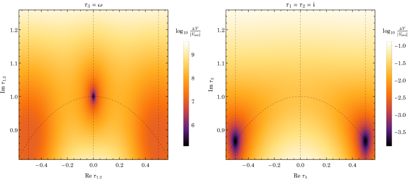
  Figure 4: Illustration for the vacua of the scalar potential in the case where $(m_{1},n_{1})=(m_{2},n_{2})=(2,0)$ and $(m_{3},n_{3})=(0,0)$. We focus on the global vacuum $(\tau_{1},\tau_{2},\tau_{3})=({\rm i},{\rm i},\omega)$. For each plot, we fix $\tau_{1}$ ($\tau_{2}$) or $\tau_{3}$ and exhibit the projection of ${\rm log}_{10}(\Delta V/|V_{\rm min}|)$ in terms of the other modulus parameter. Left Panel: $\tau_{3}=\omega$ is fixed. Right Panel: $\tau_{1}=\tau_{2}={\rm i}$ is fixed.

• If we exchange the values of $(m_{1},n_{1})$ and $(m_{3},n_{3})$, we will arrive at a mirrored case, in which similar vacua could also be easily obtained by reversing the values of $\tau_{1}$ and $\tau_{3}$. The allowed ranges of $\mathcal{A}(S,\overline{S})$ for dS vacua may change by roughly a factor of two since there are actually two moduli $\tau_{1}$ and $\tau_{2}$ associated with $(m_{1},n_{1})$.

• In the single-modulus case, it is shown $\tau={\rm i}$ will always be the minimum as long as $m>1$ Lebedev:2006qc , since the Hessian matrix is positive-definite and does not depend on $\mathcal{A}(S,\overline{S})$. However, this is not the case in the three-modulus extension. Taking $(m_{1},n_{1})=(0,0)$ and $(m_{3},n_{3})=(2,0)$ for instance, non-vanishing $H^{(0,0)}(\omega)$ recruits the dependence on $\mathcal{A}(S,\overline{S})$ in the Hessian matrix, setting an upper bound on $\mathcal{A}(S,\overline{S})$ for $\tau={\rm i}$ to be the minimum, which is of the order of $[\partial^{2}H^{(2,0)}(\tau_{i})/\partial\tau^{2}_{i}]|_{\tau_{i}={\rm i}}$.

• Among all the dS vacua, two of them are phenomenologically interesting. These two vacua appear at $\tau_{1}=\tau_{2}={\rm i}$ and $\tau_{3}=\omega$ when $(m_{1},n_{1})=(2,0)$ and $(m_{3},n_{3})=(0,0)$, and $\tau_{1}=\tau_{2}=\omega$ and $\tau_{3}={\rm i}$ when $(m_{1},n_{1})=(0,0)$ and $(m_{3},n_{3})=(2,0)$. In Fig. 4, we show the projections of ${\rm log}_{10}(\Delta V/|V_{\rm min}|)$ with the choice $(m_{1},n_{1})=(2,0)$ and $(m_{3},n_{3})=(0,0)$, by fixing respectively $\tau_{3}=\omega$ and $\tau_{1}=\tau_{2}={\rm i}$, where one can indeed find the global minimum appears when $\tau_{1}=\tau_{2}={\rm i}$ and $\tau_{3}=\omega$ in this case. In the next subsection, we will demonstrate that they can lead to viable models which can account for neutrino masses and flavour mixing.

At the end of this subsection, let us briefly discuss Class C. Although this entire non-symmetric class would be much more complicated since all the moduli should be regarded as free variables, one can still follow the similar method adopted in Class B to determine the vacua. It is shown that the vacua are still essentially located at the fixed points. Different from Class B, there may exist degenerate global minima in the fundamental domain. For example, if $(m_{1},n_{1})=(0,0)$, $(m_{2},n_{2})=(0,3)$, $(m_{3},n_{3})=(2,0)$, the global minima would appear at $\tau_{1}=\tau_{2}=\omega$ and $\tau_{3}={\rm i}$, or $\tau_{1}=\tau_{3}=\omega$ and $\tau_{2}={\rm i}$. In addition, if no pair of $(m_{i},n_{i})$ is selected to be $(0,0)$, the global minima would become Minkowski vacua.

3.3 Phenomenological implications for lepton masses and flavour mixing

The simplest factorisable compactifications with more than one torus motivate several bottom-up models based on multiple moduli fields, which can account for lepton masses, flavour mixing and CP violation deMedeirosVarzielas:2019cyj ; King:2019vhv ; King:2021fhl ; deMedeirosVarzielas:2022fbw ; deAnda:2023udh . The main idea is to introduce multiple modular symmetries, each of which is related to one modulus field. The transformation of one modulus under the corresponding modular group is independent of each other, as shown in Eq. (9). Similar to the single-modulus case, the chiral supermultiplets and Yukawa couplings are arranged as irreducible representations under different finite modular groups $\Gamma^{i}_{N_{i}}$. Here we take a minimal seesaw model based on three modular symmetries $S^{A}_{4}$, $S^{B}_{4}$ and $S^{C}_{4}$ as an example deMedeirosVarzielas:2019cyj . The moduli fields associated with three modular $S_{4}$ groups are respectively labelled by $\tau_{A}$, $\tau_{B}$ and $\tau_{C}$. The representations and modular weights of the left-handed lepton doublet $L$, three right-handed charged-lepton singlets $\{e^{c},\mu^{c},\tau^{c}\}$ (with “$c$” being the charge conjugate), two right-handed neutrino singlets $\{N^{c}_{A},N^{c}_{B}\}$, together with the Yukawa couplings and right-handed neutrino masses under the $S^{A}_{4}\times S^{B}_{4}\times S^{C}_{4}$ group are listed in Table 2. Then it is straightforward to write the superpotential relevant for the lepton masses as

$$W_{\ell} = \frac{1}{\Lambda}\left[L\Phi_{AC}Y_{A}(\tau_{A})N_{A}^{c}+L\Phi_{BC}Y_{B}(\tau_{B})N_{B}^{c}\right]H_{u}$$ (48)

$$+\left[LY_{e}(\tau_{C})e^{c}+LY_{\mu}(\tau_{C})\mu^{c}+LY_{\tau}(\tau_{C})\tau^{c}\right]H_{d}$$

$$+\frac{1}{2}M_{A}(\tau_{A})N_{A}^{c}N_{A}^{c}+\frac{1}{2}M_{B}(\tau_{B})N_{B}^{c}N_{B}^{c}+M_{AB}(\tau_{A},\tau_{B})N_{A}^{c}N_{B}^{c}\,,$$

where $H_{u,d}$ denote the Higgs doublets. It should be mentioned that two additional flavon fields $\Phi_{AC}$ and $\Phi_{BC}$ are also introduced. They behave as bi-triplets under the $S^{A}_{4}\times S^{B}_{4}\times S^{C}_{4}$ group. Once $\Phi_{AC}$ and $\Phi_{BC}$ obtain their individual VEVs, the modular $S^{A}_{4}\times S^{B}_{4}\times S^{C}_{4}$ symmetry is spontaneously broken to a unified modular $S^{D}_{4}$ symmetry, which is depicted by Fig. 5. All three moduli transform in the same way under the $S^{D}_{4}$ group. Therefore, the bi-triplet scalars play a crucial role in connecting various modular groups and accommodating all three moduli in the mass terms of charged leptons and neutrinos. The VEVs of $\Phi_{AC}$ and $\Phi_{BC}$ can be determined by introducing driving fields deMedeirosVarzielas:2019cyj , which is assumed to be independent of the modulus stabilisation.

Table 2: Representations and modular weights of leptons, Yukawa couplings $Y$ and right-handed neutrino masses $M$ in the $S_{4}^{A}\times S_{4}^{B}\times S_{4}^{C}$ group discussed in Ref. deMedeirosVarzielas:2019cyj .

Field	$S_{4}^{A}$	$S_{4}^{B}$	$S_{4}^{C}$	​$2k_{A}$​	​$2k_{B}$​	​$2k_{C}$​
$L$	$\mathbf{1}$	$\mathbf{1}$	$\mathbf{3}$	0	0	0
$e^{c}$	$\mathbf{1}$	$\mathbf{1}$	$\mathbf{1}$	0	0	​$-6$​
$\mu^{c}$	$\mathbf{1}$	$\mathbf{1}$	$\mathbf{1}$	0	0	​$-4$​
$\tau^{c}$	$\mathbf{1}$	$\mathbf{1}$	$\mathbf{1}$	0	0	​$-2$​
$N_{A}^{c}$	$\mathbf{1}$	$\mathbf{1}$	$\mathbf{1}$	​$-6$​	0	0
$N_{B}^{c}$	$\mathbf{1}$	$\mathbf{1}$	$\mathbf{1}$	0	​$-4$​	0
$\Phi_{AC}$	$\mathbf{3}$	$\mathbf{1}$	$\mathbf{3}$	0	0	0
$\Phi_{BC}$	$\mathbf{1}$	$\mathbf{3}$	$\mathbf{3}$	0	0	0

Yuk/Mass	$S_{4}^{A}$	$S_{4}^{B}$	$S_{4}^{C}$	​$2k_{A}$​	​$2k_{B}$​	​$2k_{C}$​
$Y_{e}(\tau_{C})$	$\mathbf{1}$	$\mathbf{1}$	$\mathbf{3}$	0	0	$6$
$Y_{\mu}(\tau_{C})$	$\mathbf{1}$	$\mathbf{1}$	$\mathbf{3}$	0	0	$4$
$Y_{\tau}(\tau_{C})$	$\mathbf{1}$	$\mathbf{1}$	$\mathbf{3}$	0	0	$2$
$Y_{A}(\tau_{A})$	$\mathbf{3}$	$\mathbf{1}$	$\mathbf{1}$	$6$	0	0
$Y_{B}(\tau_{B})$	$\mathbf{1}$	$\mathbf{3}$	$\mathbf{1}$	0	$4$	0
$M_{A}(\tau_{A})$	$\mathbf{1}$	$\mathbf{1}$	$\mathbf{1}$	$12$	0	0
$M_{B}(\tau_{B})$	$\mathbf{1}$	$\mathbf{1}$	$\mathbf{1}$	0	$8$	0
$M_{AB}(\tau_{A},\tau_{B})$	$\mathbf{1}$	$\mathbf{1}$	$\mathbf{1}$	$6$	$4$	0

The modulus stabilisation we have discussed in the previous sections is based on the infinite modular group $\overline{\Gamma}$. As has been shown in Fig. 6, the modulus parameter inside the fundamental domain $\mathcal{G}$ can be mapped into other domains via modular transformations, hence we should have an infinite number of degenerate vacua of $\tau$ in the upper-half complex plane. If we consider a specific finite modular group $\Gamma_{N}$, acting $\Gamma_{N}$ on $\mathcal{G}$ will give rise to the fundamental domain of $\Gamma(N)$, namely, $\mathcal{G}(N)=\Gamma_{N}\mathcal{G}$. Any transformation $\gamma\in\Gamma_{N}$ acting on $\mathcal{G}(N)$ will leave $\mathcal{G}(N)$ invariant, indicating that $\mathcal{G}(N)$ is actually a target space of $\Gamma_{N}$ deMedeirosVarzielas:2020kji . In Fig. 6, we exhibit the fundamental domain $\mathcal{G}(4)$ of $\Gamma(4)$. In order to illustrate the degeneracy of vacua inside $\mathcal{G}(4)$, we take the fixed point $\tau={\rm i}$ for instance. The red dots in Fig. 6 denotes the values of $\tau$ which can be converted to $\tau={\rm i}$ via the modular transformation $\gamma\in\Gamma_{4}$. Given that $S^{2}=(ST)^{3}=T^{4}={\bf I}$ should be satisfied, we have the following equalities

$$\begin{array}[]{rlrcccc}2+{\rm i}=&-2+{\rm i}\;,&\quad\dfrac{2}{5}+\dfrac{\rm i}{5}=&-\dfrac{2}{5}+\dfrac{\rm i}{5}\;,&\quad\dfrac{7}{5}+\dfrac{\rm i}{5}=&\dfrac{3}{5}+\dfrac{\rm i}{5}\;,\\ -\dfrac{7}{5}+\dfrac{\rm i}{5}=&-\dfrac{3}{5}+\dfrac{\rm i}{5}\;,&\quad\dfrac{8}{5}+\dfrac{\rm i}{5}=&-\dfrac{8}{5}+\dfrac{\rm i}{5}\;,\end{array}$$ (49)

indicating that there are redundant points on the boundary of $\mathcal{G}(4)$, which are represented by the hollow dots in Fig. 5. Then one can easily observe that if $\tau={\rm i}$ turns out to be the vacuum, there will be eleven additional degenerate vacua in the target space of the $S_{4}$ group. In the single-modulus case, if two moduli can be related to each other via a modular transformation, the resulting physical observables would be the same, since the modular transformation in the neutrino sector compensates for that in the charged-lepton sector and the final physical quantities will be modular-invariant. Nevertheless, if multiple moduli parameters come into the superpotential, we are unable to arbitrarily vary the values of moduli via modular transformations without changing the results of physical observables, due to the relative phases among the moduli. For example, $({\rm i},{\rm i},{\rm i})$ and $({\rm i},{\rm i},{\rm i}+2)$ would in principle result in different physical consequences.

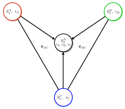
Figure 5: Illustration of the breaking of $S_{4}^{A}\times S_{4}^{B}\times S_{4}^{C}\to S_{4}^{D}$, identified as the diagonal subgroup, via the VEVs of $\Phi_{AC}$ and $\Phi_{BC}$. Figure adapted from Ref. deMedeirosVarzielas:2019cyj .

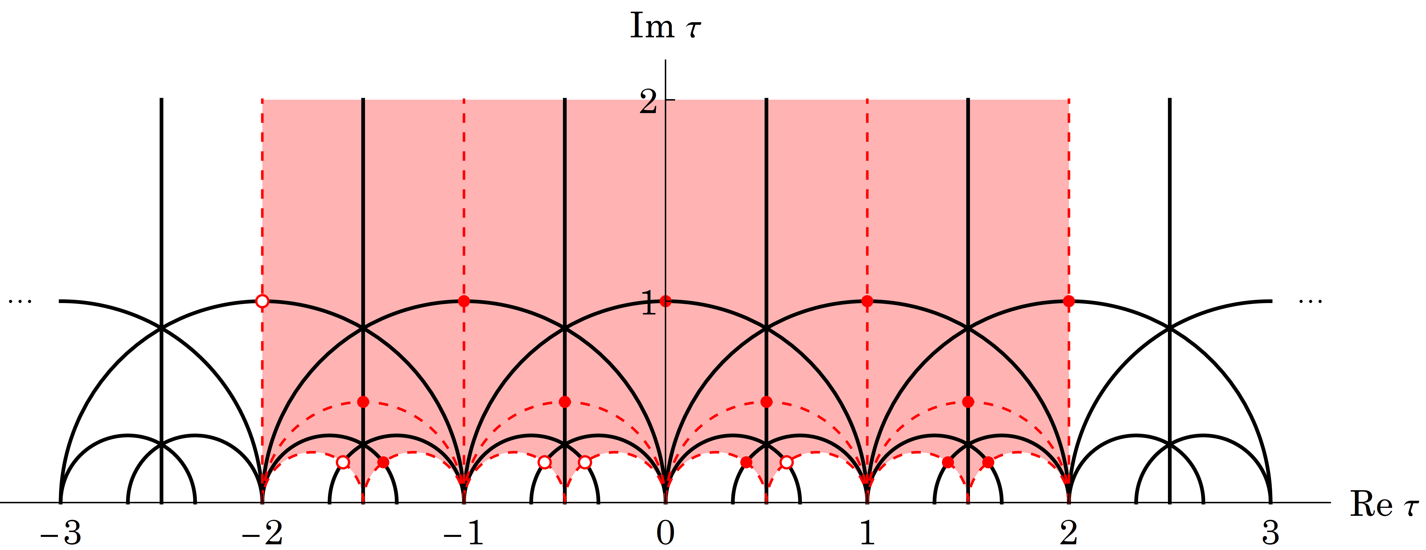
Figure 6: The fundamental domain $\mathcal{G}(4)$ of $\Gamma(4)$ is shaded by red colour. Red dots label the values of $\tau$ which can be converted to $\tau={\rm i}$ via the modular transformation $\gamma\in\Gamma_{4}$, where the hollow dots are removed due to redundancies.

In Table 3, we summarise various lepton flavour models with multiple modular symmetries, where the values of $\tau$ are taken to be precisely at the fixed points. Except for the modular $A_{5}^{l}\times A_{5}^{\nu}$ model deMedeirosVarzielas:2022ihu where the value of $\tau_{l}$ is fixed to be ${\rm i}\infty$, the VEVs of moduli required in all the other models can indeed be realised in our formalism. In particular, in the modular $S_{4}^{A}\times S_{4}^{B}\times S_{4}^{C}$ model discussed in Ref. King:2019vhv , the ${\rm TM}_{1}$ mixing pattern requires $\tau_{A}=-\omega^{2}$, $\tau_{B}=1/2+{\rm i}/2$ and $\tau_{C}=\omega$, which can be fulfilled by choosing $(m_{1},n_{1})=(m_{2},n_{2})=(0,0)$ and $(m_{3},n_{3})=(2,0)$. The littlest seesaw models can also be realised in the framework of the $S_{4}^{A}\times S_{4}^{B}\times S_{4}^{C}$ symmetry deMedeirosVarzielas:2022fbw ; deAnda:2023udh ; deMedeirosVarzielas:2023ujt , where the required VEVs of moduli can be generated by choosing $(m_{1},n_{1})=(m_{2},n_{2})=(2,0)$ and $(m_{3},n_{3})=(0,0)$. Therefore we indeed find a dynamical origin of the VEVs of moduli fields in the modular-invariant models with multiple moduli.

Table 3: Models with multiple modular symmetries investigated in the previous literature. The values of moduli parameters in the charged-lepton and neutrino sectors that can generate viable lepton masses and flavour mixing, together with the corresponding flavour mixing patterns are summarised.

Modular group	Charged-lepton sector	Neutrino sector	Flavour pattern	References
$S_{4}^{A}\times S_{4}^{B}\times S_{4}^{C}$	$\tau_{C}=\omega$	$\tau_{A}=-\omega^{2}$, $\tau_{B}=\dfrac{1}{2}+\dfrac{\rm i}{2}$	${\rm TM}_{1}$	Ref. deMedeirosVarzielas:2019cyj
$S_{4}^{l}\times S_{4}^{\nu}$	$\tau_{l}=\omega$	$\tau_{\nu}=-\dfrac{1}{2}+\dfrac{\rm i}{2}$	${\rm TM}_{1}$	Ref. King:2019vhv
$S^{F}_{4}\times S^{N}_{4}$	$\tau_{F}=\omega$	$\tau_{N}=-\dfrac{1}{2}+\dfrac{\rm i}{2}$	CM + ${\rm TM}_{1}$	Ref. King:2021fhl
$S_{4}^{A}\times S_{4}^{B}\times S_{4}^{C}$	$\tau_{C}=\omega$	$\tau_{A}=\dfrac{1}{2}+\dfrac{\rm i}{2}$, $\tau_{B}=\dfrac{3}{2}+\dfrac{\rm i}{2}$	Littlest modular seesaw	Refs. deMedeirosVarzielas:2022fbw ; deMedeirosVarzielas:2023ujt
$S_{4}^{A}\times S_{4}^{B}\times S_{4}^{C}$	$\tau_{C}=\omega$	$\tau_{A}={\rm i}+2$, $\tau_{B}={\rm i}$	Littlest modular seesaw	Ref. deAnda:2023udh
$A_{4}^{l}\times A_{4}^{\nu}$	$\tau_{l}=\dfrac{3}{2}+\dfrac{\rm i}{2\sqrt{3}}$	$\tau_{\nu}={\rm i}$	${\rm TM}_{2}$	Ref. deMedeirosVarzielas:2021pug
$A_{5}^{l}\times A_{5}^{\nu}$	$\tau_{l}={\rm i}\infty$	$\tau_{\nu}={\rm i}$	${\rm GR}_{2}$	Ref. deMedeirosVarzielas:2022ihu

4 Summary

The modular symmetry provides us with a satisfactory and appealing framework for addressing the flavour problem. The only flavons present in such a framework are one or more moduli fields $\tau$. It seems that the fixed points $\tau={\rm i}$ and $\tau=\omega$ play a special role in both the phenomenological model building and the 10d supersymmetric orbifold examples. However, revealing the origin of the VEVs of moduli is still an intricate challenge.

In this paper, we study the modulus stabilisation within the multiple-modulus framework. In line with Ref. Leedom:2022zdm , we consider the Kähler moduli and dilaton but neglect their coupling with matter fields. The influence of the dilaton sector is two-fold. On the one hand, the tree-level dilaton Kähler potential will be modified by additional non-perturbative stringy effects, e.g., Shenker-like effects, which are vital for us to evade several dS no-go theorems. On the other hand, the dilaton will enter the superpotential as a functional form $\Omega(S)$. The parameterised form of the superpotential turns out to be Eq. (40), where the modular-invariant function $H(\tau)$ in the single-modulus case is replaced by ${\mathcal{H}}(\tau_{1},\tau_{2},\tau_{3})=H^{(m_{1},n_{1})}(\tau_{1})+H^{(m_{2},n_{2})}(\tau_{2})+H^{(m_{3},n_{3})}(\tau_{3})$ in the three-modulus case. The scalar potential in the three-modulus scenario is then given by Eq. (41), where the contribution from the dilaton sector is parameterised by $\mathcal{A}(S,\overline{S})$.

We numerically search the minima of the scalar potential in the entire parameter space of $\tau_{i}$ and $\mathcal{A}(S,\overline{S})$, and calculate the Hessian matrices at the fixed points $\tau={\rm i}$ and $\omega$. Due to the existence of additional Kähler moduli, the vacua look rather different from those in the single-modulus case. In fact, both the finite fixed points $\tau={\rm i}$ and $\tau=\omega$ could be the dS vacua of the scalar potential if specific conditions on $\mathcal{A}(S,\overline{S})$ are satisfied. We classify different choices of vacua by varying the indices $(m_{i},n_{i})$, and summarise conditions for the vacua to be dS minima in Table 1, which are also distinct from the single modulus case. In addition, we are unable to obtain the dS vacua which are close to but not precisely at the fixed points within this framework.

Modulus stabilisation discussed in this paper has significant phenomenological implications for fermion masses and flavour mixing, once the finite modular groups are specified. In particular, we find that the vacua $(\tau_{1},\tau_{2},\tau_{3})=(\omega,\omega,{\rm i})$ [obtained by setting $(m_{1},n_{1})=(m_{2},n_{2})=(0,0)$ and $(m_{3},n_{3})=(2,0)$] and $(\tau_{1},\tau_{2},\tau_{3})=({\rm i},{\rm i},\omega)$ [obtained by setting $(m_{1},n_{1})=(m_{2},n_{2})=(2,0)$ and $(m_{3},n_{3})=(0,0)$] can lead to the ${\rm TM}_{1}$ mixing and littlest modular seesaw model, respectively. It should be mentioned that there are several degenerate vacua inside the fundamental domain $\mathcal{G}(N)$ of $\Gamma(N)$. Therefore it would be interesting to explore whether the domain wall problem could exist and how to break this degeneracy, which we leave for future work.

Appendix A Why is the scalar potential modular-invariant?

Before going further, it is useful to find out how the derivative of modular forms changes under the modular transformation. Suppose $f(\tau)$ is a modular form, we have

$$\begin{split}f^{\prime}(\tau)\equiv\frac{\rm d}{{\rm d}\tau}f(\tau)\stackrel{{\scriptstyle\gamma}}{{\rightarrow}}\frac{\rm d}{{\rm d}(\gamma\tau)}f(\gamma\tau)&=\frac{\rm d}{{\rm d}\tau}\left[(c\tau+d)^{k}f(\tau)\right]\cdot\frac{{\rm d}\tau}{{\rm d}(\gamma\tau)}\\ &=ck(c\tau+d)^{k+1}f(\tau)+(c\tau+d)^{k+2}f^{\prime}(\tau)\;,\end{split}$$ (50)

where we have used the relations

$$\gamma\tau=\frac{a\tau+b}{c\tau+d}\;,\quad{\rm d}(\gamma\tau)=\frac{{\rm d}\tau}{(c\tau+d)^{2}}\;.$$ (51)

From Eq. (50) we can easily find that $f^{\prime}(\tau)$ becomes a modular form with weight two only if $f(\tau)$ is a zero-weight modular form. In this regard, we introduce the derivative $D_{i}$ which is covariant under the modular transformation. Keeping Eq. (14) in mind, we find that

$$D_{i}{\cal W}=\partial_{i}{\cal W}+(\partial_{i}{\cal K}){\cal W}=\partial_{i}{\cal W}+(\partial_{i}G-\partial_{i}\log|{\cal W}|^{2}){\cal W}=(\partial_{i}G){\cal W}\;.$$ (52)

Since $G$ is a modular-invariant function, i.e., a modular form with weight zero, $D_{i}{\cal W}$ then turns out to be a modular form with $k=-1$.

Now we can write down the transformation properties of all the components in the scalar potential

$$\begin{split}e^{{\cal K}}&\to(c\tau+d)^{6}e^{{\cal K}}\;,\\ {\cal K}^{i\overline{j}}&\to|c\tau+d|^{-4}{\cal K}^{i\overline{j}}\;,\\ D_{i}{\cal W}&\to(c\tau+d)^{-1}D_{i}{\cal W}\;.\end{split}$$ (53)

Taking the above transformation rules into consideration, we can conclude that the scalar potential $V$ is indeed invariant under the modular transformation.

Appendix B The Dedekind $\eta$ function and Klein $j$ function

In this appendix, we present the definitions of several important modular forms. The Dedekind $\eta$ function is a modular form with a weight of $-1/2$ defined as

$$\eta(\tau)\equiv q^{1/24}\prod_{n=1}^{\infty}\left(1-q^{n}\right)\;,$$ (54)

where $q=e^{2\pi{\rm i}\tau}$. One can express $\eta(\tau)$ as the following $q$-expansions

$$\eta=q^{1/24}\left(1-q-q^{2}+q^{5}+q^{7}-q^{12}-q^{15}+\mathcal{O}\left(q^{22}\right)\right)\;.$$ (55)

The Eisenstein series $G_{2k}(\tau)$ is another kind of modular form with a weight of $2k$, the definition of which is

$$G_{2k}(\tau)=\sum_{\begin{subarray}{c}n_{1},n_{2}\in\mathbb{Z}\\ \left(n_{1},n_{2}\right)\neq(0,0)\end{subarray}}\left(n_{1}+n_{2}\tau\right)^{-2k}\;,$$ (56)

which converges to the holomorphic function in the upper-half complex plane for the integer $k\geq 2$. The series does not converge when $k=1$, but one can still define $G_{2}(\tau)$ via a specific prescription on the order of summation. With the help of $\eta(\tau)$ and $G_{4}(\tau)$, one can define a modular-invariant function which is called the Klein $j$ function as

$$j(\tau)=\frac{3^{6}5^{3}}{\pi^{12}}\frac{G_{4}(\tau)^{3}}{\eta(\tau)^{24}}\;,$$ (57)

which is also a modular form with weight zero.

References

- (1) S.F. King and C. Luhn, Neutrino Mass and Mixing with Discrete Symmetry, Rept. Prog. Phys. 76 (2013) 056201 [1301.1340].
- (2) F. Feruglio, Are neutrino masses modular forms?, in From My Vast Repertoire …: Guido Altarelli’s Legacy, A. Levy, S. Forte and G. Ridolfi, eds., pp. 227–266 (2019), DOI [1706.08749].
- (3) S. Ferrara, D. Lust, A.D. Shapere and S. Theisen, Modular Invariance in Supersymmetric Field Theories, Phys. Lett. B 225 (1989) 363.
- (4) S. Ferrara, .D. Lust and S. Theisen, Target Space Modular Invariance and Low-Energy Couplings in Orbifold Compactifications, Phys. Lett. B 233 (1989) 147.
- (5) K. Ishiguro, T. Kobayashi and H. Otsuka, Symplectic modular symmetry in heterotic string vacua: flavor, CP, and R-symmetries, JHEP 01 (2022) 020 [2107.00487].
- (6) D. Cremades, L.E. Ibanez and F. Marchesano, Computing Yukawa couplings from magnetized extra dimensions, JHEP 05 (2004) 079 [hep-th/0404229].
- (7) K. Ishiguro, T. Kobayashi and H. Otsuka, Landscape of Modular Symmetric Flavor Models, JHEP 03 (2021) 161 [2011.09154].
- (8) T. Kobayashi, K. Tanaka and T.H. Tatsuishi, Neutrino mixing from finite modular groups, Phys. Rev. D 98 (2018) 016004 [1803.10391].
- (9) J.C. Criado and F. Feruglio, Modular Invariance Faces Precision Neutrino Data, SciPost Phys. 5 (2018) 042 [1807.01125].
- (10) T. Kobayashi, N. Omoto, Y. Shimizu, K. Takagi, M. Tanimoto and T.H. Tatsuishi, Modular A4 invariance and neutrino mixing, JHEP 11 (2018) 196 [1808.03012].
- (11) F.J. de Anda, S.F. King and E. Perdomo, grand unified theory with modular symmetry, Phys. Rev. D 101 (2020) 015028 [1812.05620].
- (12) H. Okada and M. Tanimoto, CP violation of quarks in modular invariance, Phys. Lett. B 791 (2019) 54 [1812.09677].
- (13) H. Okada and M. Tanimoto, Towards unification of quark and lepton flavors in modular invariance, Eur. Phys. J. C 81 (2021) 52 [1905.13421].
- (14) T. Nomura and H. Okada, A two loop induced neutrino mass model with modular symmetry, Nucl. Phys. B 966 (2021) 115372 [1906.03927].
- (15) G.-J. Ding, S.F. King, X.-G. Liu and J.-N. Lu, Modular S4 and A4 symmetries and their fixed points: new predictive examples of lepton mixing, JHEP 12 (2019) 030 [1910.03460].
- (16) G.-J. Ding, S.F. King and X.-G. Liu, Modular A4 symmetry models of neutrinos and charged leptons, JHEP 09 (2019) 074 [1907.11714].
- (17) D. Zhang, A modular symmetry realization of two-zero textures of the Majorana neutrino mass matrix, Nucl. Phys. B 952 (2020) 114935 [1910.07869].
- (18) T. Kobayashi, T. Nomura and T. Shimomura, Type II seesaw models with modular symmetry, Phys. Rev. D 102 (2020) 035019 [1912.00637].
- (19) X. Wang, Lepton flavor mixing and CP violation in the minimal type-(I+II) seesaw model with a modular symmetry, Nucl. Phys. B 957 (2020) 115105 [1912.13284].
- (20) H. Okada and M. Tanimoto, Quark and lepton flavors with common modulus in A4 modular symmetry, Phys. Dark Univ. 40 (2023) 101204 [2005.00775].
- (21) C.-Y. Yao, J.-N. Lu and G.-J. Ding, Modular Invariant Models for Quarks and Leptons with Generalized CP Symmetry, JHEP 05 (2021) 102 [2012.13390].
- (22) P. Chen, G.-J. Ding and S.F. King, SU(5) GUTs with A4 modular symmetry, JHEP 04 (2021) 239 [2101.12724].
- (23) T. Kobayashi, H. Otsuka, M. Tanimoto and K. Yamamoto, Modular symmetry in the SMEFT, Phys. Rev. D 105 (2022) 055022 [2112.00493].
- (24) D.W. Kang, J. Kim, T. Nomura and H. Okada, Natural mass hierarchy among three heavy Majorana neutrinos for resonant leptogenesis under modular A4 symmetry, JHEP 07 (2022) 050 [2205.08269].
- (25) J.T. Penedo and S.T. Petcov, Lepton Masses and Mixing from Modular Symmetry, Nucl. Phys. B 939 (2019) 292 [1806.11040].
- (26) P.P. Novichkov, J.T. Penedo, S.T. Petcov and A.V. Titov, Modular S4 models of lepton masses and mixing, JHEP 04 (2019) 005 [1811.04933].
- (27) T. Kobayashi, Y. Shimizu, K. Takagi, M. Tanimoto and T.H. Tatsuishi, New lepton flavor model from modular symmetry, JHEP 02 (2020) 097 [1907.09141].
- (28) X. Wang and S. Zhou, The minimal seesaw model with a modular S4 symmetry, JHEP 05 (2020) 017 [1910.09473].
- (29) P.P. Novichkov, J.T. Penedo, S.T. Petcov and A.V. Titov, Modular A5 symmetry for flavour model building, JHEP 04 (2019) 174 [1812.02158].
- (30) G.-J. Ding, S.F. King and X.-G. Liu, Neutrino mass and mixing with modular symmetry, Phys. Rev. D 100 (2019) 115005 [1903.12588].
- (31) J.C. Criado, F. Feruglio and S.J.D. King, Modular Invariant Models of Lepton Masses at Levels 4 and 5, JHEP 02 (2020) 001 [1908.11867].
- (32) X.-G. Liu and G.-J. Ding, Neutrino Masses and Mixing from Double Covering of Finite Modular Groups, JHEP 08 (2019) 134 [1907.01488].
- (33) H. Okada and Y. Orikasa, Lepton mass matrix from double covering of A 4 modular flavor symmetry*, Chin. Phys. C 46 (2022) 123108 [2206.12629].
- (34) G.-J. Ding, F.R. Joaquim and J.-N. Lu, Texture-zero patterns of lepton mass matrices from modular symmetry, JHEP 03 (2023) 141 [2211.08136].
- (35) P. Mishra, M.K. Behera and R. Mohanta, Neutrino phenomenology, W-mass anomaly, and muon (g-2) in a minimal type-III seesaw model using a T’ modular symmetry, Phys. Rev. D 107 (2023) 115004 [2302.00494].
- (36) G.-J. Ding, S.F. King, C.-C. Li, X.-G. Liu and J.-N. Lu, Neutrino mass and mixing models with eclectic flavor symmetry (27) T’, JHEP 05 (2023) 144 [2303.02071].
- (37) P.P. Novichkov, J.T. Penedo and S.T. Petcov, Double cover of modular for flavour model building, Nucl. Phys. B 963 (2021) 115301 [2006.03058].
- (38) X.-G. Liu, C.-Y. Yao and G.-J. Ding, Modular invariant quark and lepton models in double covering of modular group, Phys. Rev. D 103 (2021) 056013 [2006.10722].
- (39) G.-J. Ding, X.-G. Liu and C.-Y. Yao, A minimal modular invariant neutrino model, JHEP 01 (2023) 125 [2211.04546].
- (40) X. Wang, B. Yu and S. Zhou, Double covering of the modular group and lepton flavor mixing in the minimal seesaw model, Phys. Rev. D 103 (2021) 076005 [2010.10159].
- (41) C.-Y. Yao, X.-G. Liu and G.-J. Ding, Fermion masses and mixing from the double cover and metaplectic cover of the modular group, Phys. Rev. D 103 (2021) 095013 [2011.03501].
- (42) M.K. Behera and R. Mohanta, Inverse seesaw in modular symmetry, J. Phys. G 49 (2022) 045001 [2108.01059].
- (43) C.-C. Li, X.-G. Liu and G.-J. Ding, Modular symmetry at level 6 and a new route towards finite modular groups, JHEP 10 (2021) 238 [2108.02181].
- (44) Y. Abe, T. Higaki, J. Kawamura and T. Kobayashi, Fermion hierarchies in SU(5) grand unification from modular flavor symmetry, JHEP 08 (2023) 097 [2307.01419].
- (45) Y. Abe, T. Higaki, J. Kawamura and T. Kobayashi, Quark and lepton hierarchies from S4’ modular flavor symmetry, Phys. Lett. B 842 (2023) 137977 [2302.11183].
- (46) P.P. Novichkov, S.T. Petcov and M. Tanimoto, Trimaximal Neutrino Mixing from Modular A4 Invariance with Residual Symmetries, Phys. Lett. B 793 (2019) 247 [1812.11289].
- (47) I. de Medeiros Varzielas, M. Levy and Y.-L. Zhou, Symmetries and stabilisers in modular invariant flavour models, JHEP 11 (2020) 085 [2008.05329].
- (48) P.P. Novichkov, J.T. Penedo and S.T. Petcov, Fermion mass hierarchies, large lepton mixing and residual modular symmetries, JHEP 04 (2021) 206 [2102.07488].
- (49) S.T. Petcov and M. Tanimoto, modular flavour model of quark mass hierarchies close to the fixed point , Eur. Phys. J. C 83 (2023) 579 [2212.13336].
- (50) S.T. Petcov and M. Tanimoto, A4 modular flavour model of quark mass hierarchies close to the fixed point = i, JHEP 08 (2023) 086 [2306.05730].
- (51) H. Okada and M. Tanimoto, Modular invariant flavor model of and hierarchical structures at nearby fixed points, Phys. Rev. D 103 (2021) 015005 [2009.14242].
- (52) X. Wang and S. Zhou, Explicit perturbations to the stabilizer = i of modular symmetry and leptonic CP violation, JHEP 07 (2021) 093 [2102.04358].
- (53) F. Feruglio, V. Gherardi, A. Romanino and A. Titov, Modular invariant dynamics and fermion mass hierarchies around , JHEP 05 (2021) 242 [2101.08718].
- (54) S. Kikuchi, T. Kobayashi, M. Tanimoto and H. Uchida, Texture zeros of quark mass matrices at fixed point in modular flavor symmetry, Eur. Phys. J. C 83 (2023) 591 [2207.04609].
- (55) F. Feruglio, Universal Predictions of Modular Invariant Flavor Models near the Self-Dual Point, Phys. Rev. Lett. 130 (2023) 101801 [2211.00659].
- (56) F. Feruglio, Fermion masses, critical behavior and universality, JHEP 03 (2023) 236 [2302.11580].
- (57) I. de Medeiros Varzielas, M. Levy, J.T. Penedo and S.T. Petcov, Quarks at the modular S4 cusp, JHEP 09 (2023) 196 [2307.14410].
- (58) S. Kikuchi, T. Kobayashi, K. Nasu, S. Takada and H. Uchida, Quark mass hierarchies and CP violation in A4 × A4 × A4 modular symmetric flavor models, JHEP 07 (2023) 134 [2302.03326].
- (59) Y. Abe, T. Higaki, J. Kawamura and T. Kobayashi, Quark masses and CKM hierarchies from modular flavor symmetry, 2301.07439.
- (60) S.J.D. King and S.F. King, Fermion mass hierarchies from modular symmetry, JHEP 09 (2020) 043 [2002.00969].
- (61) I. de Medeiros Varzielas, S.F. King and Y.-L. Zhou, Multiple modular symmetries as the origin of flavor, Phys. Rev. D 101 (2020) 055033 [1906.02208].
- (62) S.F. King and Y.-L. Zhou, Trimaximal TM1 mixing with two modular groups, Phys. Rev. D 101 (2020) 015001 [1908.02770].
- (63) S.F. King and Y.-L. Zhou, Twin modular S4 with SU(5) GUT, JHEP 04 (2021) 291 [2103.02633].
- (64) I. de Medeiros Varzielas, S.F. King and M. Levy, Littlest modular seesaw, JHEP 02 (2023) 143 [2211.00654].
- (65) F.J. de Anda and S.F. King, Modular flavour symmetry and orbifolds, JHEP 06 (2023) 122 [2304.05958].
- (66) I. de Medeiros Varzielas and J.a. Lourenço, Two A4 modular symmetries for Tri-Maximal 2 mixing, Nucl. Phys. B 979 (2022) 115793 [2107.04042].
- (67) I. de Medeiros Varzielas and J.a. Lourenço, Two A5 modular symmetries for Golden Ratio 2 mixing, Nucl. Phys. B 984 (2022) 115974 [2206.14869].
- (68) I. de Medeiros Varzielas, S.F. King and M. Levy, A Modular Littlest Seesaw, 2309.15901.
- (69) M. Fischer, M. Ratz, J. Torrado and P.K.S. Vaudrevange, Classification of symmetric toroidal orbifolds, JHEP 01 (2013) 084 [1209.3906].
- (70) M. Cicoli, J.P. Conlon, A. Maharana, S. Parameswaran, F. Quevedo and I. Zavala, String Cosmology: from the Early Universe to Today, 2303.04819.
- (71) S.B. Giddings, S. Kachru and J. Polchinski, Hierarchies from fluxes in string compactifications, Phys. Rev. D 66 (2002) 106006 [hep-th/0105097].
- (72) S. Gukov, C. Vafa and E. Witten, CFT’s from Calabi-Yau four folds, Nucl. Phys. B 584 (2000) 69 [hep-th/9906070].
- (73) G. Curio, A. Klemm, D. Lust and S. Theisen, On the vacuum structure of type II string compactifications on Calabi-Yau spaces with H fluxes, Nucl. Phys. B 609 (2001) 3 [hep-th/0012213].
- (74) S. Ashok and M.R. Douglas, Counting flux vacua, JHEP 01 (2004) 060 [hep-th/0307049].
- (75) F. Denef and M.R. Douglas, Distributions of nonsupersymmetric flux vacua, JHEP 03 (2005) 061 [hep-th/0411183].
- (76) T. Kobayashi, Y. Shimizu, K. Takagi, M. Tanimoto and T.H. Tatsuishi, lepton flavor model and modulus stabilization from modular symmetry, Phys. Rev. D 100 (2019) 115045 [1909.05139].
- (77) T. Kobayashi, Y. Shimizu, K. Takagi, M. Tanimoto, T.H. Tatsuishi and H. Uchida, violation in modular invariant flavor models, Phys. Rev. D 101 (2020) 055046 [1910.11553].
- (78) M. Dine, R. Rohm, N. Seiberg and E. Witten, Gluino Condensation in Superstring Models, Phys. Lett. B 156 (1985) 55.
- (79) H.P. Nilles, Dynamically Broken Supergravity and the Hierarchy Problem, Phys. Lett. B 115 (1982) 193.
- (80) S. Ferrara, L. Girardello and H.P. Nilles, Breakdown of Local Supersymmetry Through Gauge Fermion Condensates, Phys. Lett. B 125 (1983) 457.
- (81) V.S. Kaplunovsky, One Loop Threshold Effects in String Unification, Nucl. Phys. B 307 (1988) 145 [hep-th/9205068].
- (82) L.J. Dixon, V. Kaplunovsky and J. Louis, Moduli dependence of string loop corrections to gauge coupling constants, Nucl. Phys. B 355 (1991) 649.
- (83) I. Antoniadis, K.S. Narain and T.R. Taylor, Higher genus string corrections to gauge couplings, Phys. Lett. B 267 (1991) 37.
- (84) I. Antoniadis, E. Gava and K.S. Narain, Moduli corrections to gauge and gravitational couplings in four-dimensional superstrings, Nucl. Phys. B 383 (1992) 93 [hep-th/9204030].
- (85) M. Cicoli, S. de Alwis and A. Westphal, Heterotic Moduli Stabilisation, JHEP 10 (2013) 199 [1304.1809].
- (86) A. Font, L.E. Ibanez, D. Lust and F. Quevedo, Supersymmetry Breaking From Duality Invariant Gaugino Condensation, Phys. Lett. B 245 (1990) 401.
- (87) E. Gonzalo, L.E. Ibáñez and A.M. Uranga, Modular symmetries and the swampland conjectures, JHEP 05 (2019) 105 [1812.06520].
- (88) P.P. Novichkov, J.T. Penedo and S.T. Petcov, Modular flavour symmetries and modulus stabilisation, JHEP 03 (2022) 149 [2201.02020].
- (89) V. Knapp-Perez, X.-G. Liu, H.P. Nilles, S. Ramos-Sanchez and M. Ratz, Matter matters in moduli fixing and modular flavor symmetries, 2304.14437.
- (90) O. Lebedev, H.P. Nilles and M. Ratz, De Sitter vacua from matter superpotentials, Phys. Lett. B 636 (2006) 126 [hep-th/0603047].
- (91) O. Lebedev, V. Lowen, Y. Mambrini, H.P. Nilles and M. Ratz, Metastable Vacua in Flux Compactifications and Their Phenomenology, JHEP 02 (2007) 063 [hep-ph/0612035].
- (92) J.M. Leedom, N. Righi and A. Westphal, Heterotic de Sitter beyond modular symmetry, JHEP 02 (2023) 209 [2212.03876].
- (93) S. ShenkerThe Strength of Nonperturbative Effects in String Theory, Random Surfaces and Quantum Gravity (1990) 191.
- (94) E. Cremmer, S. Ferrara, L. Girardello and A. Van Proeyen, Yang-Mills Theories with Local Supersymmetry: Lagrangian, Transformation Laws and SuperHiggs Effect, Nucl. Phys. B 212 (1983) 413.
- (95) J.P. Derendinger, S. Ferrara, C. Kounnas and F. Zwirner, On loop corrections to string effective field theories: Field dependent gauge couplings and sigma model anomalies, Nucl. Phys. B 372 (1992) 145.
- (96) D. Lust and C. Munoz, Duality invariant gaugino condensation and one loop corrected Kahler potentials in string theory, Phys. Lett. B 279 (1992) 272 [hep-th/9201047].
- (97) G. Lopes Cardoso and B.A. Ovrut, A Green-Schwarz mechanism for D = 4, N=1 supergravity anomalies, Nucl. Phys. B 369 (1992) 351.
- (98) G. Lopes Cardoso and B.A. Ovrut, Coordinate and Kahler sigma model anomalies and their cancellation in string effective field theories, Nucl. Phys. B 392 (1993) 315 [hep-th/9205009].
- (99) V. Kaplunovsky and J. Louis, On Gauge couplings in string theory, Nucl. Phys. B 444 (1995) 191 [hep-th/9502077].
- (100) M. Cvetic, A. Font, L.E. Ibanez, D. Lust and F. Quevedo, Target space duality, supersymmetry breaking and the stability of classical string vacua, Nucl. Phys. B 361 (1991) 194.