A CJ-FEAST GSVDsolver for computing a partial GSVD of a large matrix pair with the generalized singular values in a given interval

Abstract

We propose a CJ-FEAST GSVDsolver to compute a partial generalized singular value decomposition (GSVD) of a large matrix pair $(A,B)$ with the generalized singular values in a given interval. The solver is a highly nontrivial extension of the FEAST eigensolver for the (generalized) eigenvalue problem and CJ-FEAST SVDsolver for the SVD problem. For a partial GSVD problem, given three left and right searching subspaces, we propose a general projection method that works on $(A,B)$ directly, and computes approximations to the desired GSVD components. For the concerning GSVD problem, we exploit the Chebyshev–Jackson (CJ) series to construct an approximate spectral projector of the generalized eigenvalue problem of the matrix pair $(A^{T}A,B^{T}B)$ associated with the generalized singular values of interest, and use subspace iteration on it to generate a right subspace. Premultiplying it with $A$ and $B$ constructs two left subspaces. Applying the general projection method to the subspaces constructed leads to the CJ-FEAST GSVDsolver. We derive accuracy estimates for the approximate spectral projector and its eigenvalues, and establish a number of convergence results on the underlying subspaces and the approximate GSVD components obtained by the CJ-FEAST GSVDsolver. We propose general-purpose choice strategies for the series degree and subspace dimension. Numerical experiments illustrate the efficiency of the CJ-FEAST GSVDsolver.

15A18, 65F15, 65F50

1 Introduction

The generalized singular value decomposition (GSVD) of a matrix pair $(A,B)$ was introduced by Van Loan [43] and developed by Paige and Saunders [28]. It is a generalization of the singular value decomposition (SVD) of a single matrix to a matrix pair, and has been a standard matrix decomposition [3, 7, 38, 39]. The GSVD not only provides us with an important mathematical tool but also plays a key role in a number of disciplines and scientific computing, e.g., linear discrete ill-posed problems with general-form regularization [10], weighted least squares and total least squares problems [3], information retrieval, linear discriminant analysis, and many others [42].

Let $A\in\mathbb{R}^{m_{1}\times n}$ and $B\in\mathbb{R}^{m_{2}\times n}$ with $m_{1}+m_{2}\geq n$, and assume that the stacked matrix $[A^{T},B^{T}]^{T}$ has full column rank with the superscript $T$ the transpose of a matrix, i.e., the null space intersection $\mathcal{N}(A)\cap\mathcal{N}(B)=\{\textbf{0}\}$. Then the pair $(A,B)$ is called regular, the same terminology as for the generalized eigenvalue problem [40]. Denote $q_{1}=\dim(\mathcal{N}(A))$ and $q_{2}=\dim(\mathcal{N}(B))$, $q=n-q_{1}-q_{2}$, and $l_{1}=\dim(\mathcal{N}(A^{T}))$ and $l_{2}=\dim(\mathcal{N}(B^{T}))$. Then the GSVD of $(A,B)$ is

(1) $$\begin{cases}U^{T}AX=\Sigma_{A}=\operatorname{diag}\{C_{A},\mathbf{0}_{l_{1},q_{1}},I_{q_{2}}\},\\ V^{T}BX=\Sigma_{B}=\operatorname{diag}\{S_{B},I_{q_{1}},\mathbf{0}_{l_{2},q_{2}}\},\end{cases}$$

where $X=[X_{q},X_{q_{1}},X_{q_{2}}]$ is nonsingular, $U=[U_{q},U_{l_{1}},U_{q_{2}}]$ and $V=[V_{q},V_{q_{1}},V_{l_{2}}]$ are orthogonal, and the diagonal $C_{A}=\operatorname{diag}\{c_{1},\dots,c_{q}\}$ and $S_{B}=\operatorname{diag}\{s_{1},\dots,s_{q}\}$ satisfy

$$0<c_{i},s_{i}<1\quad\mbox{and}\quad c_{i}^{2}+s_{i}^{2}=1,\quad i=1,\dots,q;$$

see [7, p. 309]. In order to distinguish the block submatrices of $X,U,V$, we have denoted by the subscripts their column numbers, by $I_{k}$ and $\mathbf{0}_{k,l}$ the identity matrix of order $k$ and zero matrix of order $k\times l$, respectively, with the subscript $k$ dropped whenever it is clear from the context, and by $e_{i}$ the $i$th column of $I$.

We call the pairs $\{c_{i},s_{i}\}$ or $\sigma_{i}=c_{i}/s_{i},\ i=1,2,\ldots,q$ the nontrivial generalized singular values of $(A,B)$ and the corresponding columns $u_{i},v_{i},x_{i}$ of $U_{q},V_{q}$ and $X_{q}$ the left and right generalized singular vectors. The partitioned matrix $[X_{q_{1}},X_{q_{2}}]$ corresponds to the trivial $q_{1}$ multiple zero and $q_{2}$ multiple infinite generalized singular values, written as $\{c,s\}=\{0,1\}$ and $\{c,s\}=\{1,0\}$, respectively. We will order the $q$ generalized singular values $\{c_{i},s_{i}\}$ later. It follows from (1) that $X^{T}(A^{T}A+B^{T}B)X=I_{n}$; that is, $X$ is $(A^{T}A+B^{T}B)$-orthogonal, and its columns are $(A^{T}A+B^{T}B)$-orthonormal. If both $A$ and $B$ are of full column rank, then $q=n$.

In this paper, we are concerned with the computation of a partial GSVD of a large regular $(A,B)$ with all the generalized singular values $\sigma_{i}$ in a given interval. In terms of the one-to-one correspondence of $c$ and $\sigma$ with subscripts $i$ dropped, this amounts to the problem: Given an interval $[c_{\min},c_{\max}]\subset(0,1)$, we want to compute all the $n_{gv}$ generalized singular quintuples $(c,s,u,v,x)$, called the GSVD components, with $c\in[c_{\min},c_{\max}]$. Keep in mind that, in terms of GSVD (1), the GSVD components can be written in the matrix-vector form:

(2) $$\begin{cases}Ax=cu,\\ Bx=sv,\\ sA^{T}u=cB^{T}v.\end{cases}$$

Unlike a partial SVD of a single large matrix, not much work has been done for the partial GSVD computation of the large matrix pair $(A,B)$. Zha [44] proposes a joint bidiagonalization (JBD) method to compute a few extreme GSVD components of $(A,B)$. The method is based on a JBD process that successively reduces $(A,B)$ to a sequence of upper bidiagonal pairs, from which approximate GSVD components are computed. Kilmer, Hansen and Español [26] adapt the JBD process to the linear discrete ill-posed problem with general-form regularization, and develop a variant of the JBD process that reduces $(A,B)$ to lower-upper bidiagonal forms. Based on it, they propose a hybrid projection method. Jia and Yang [22] present a new JBD process based iterative algorithm for the ill-posed problem, which is simpler and cheaper than and computes a regularized solution at least as accurately as the hybrid method in [26]. They have considered the convergence of extreme generalized singular values. Jia and Li [21] have made a detailed numerical analysis on the JBD method for the GSVD computation and shown that it suffices to maintain the semi-orthogonality of the four sets of computed Lanczos-type vectors in finite precision arithmetic when computing generalized singular values accurately, where the semi-orthogonality means that two vectors are numerically orthogonal to the level of $\epsilon_{\mathrm{mach}}^{1/2}$ with $\epsilon_{\mathrm{mach}}$ being the machine precision. Jia and Li [20] propose an effective and efficient partial reorthogonalization strategy to maintain the desired semi-orthogonality so as to avoid convergence delay and the appearance of duplicate approximate generalized singular values. To be practical, Alvarruiz, Campos and Roman [1] have recently developed an explicit thick-restart JBD algorithm for the GSVD computation.

Hochstenbach [11] presents a Jacobi–Davidson (JD) GSVD (JDGSVD) method to compute a number of GSVD components of $(A,B)$ with the desired generalized singular values closest to a given target. The method formulates the GSVD of $(A,B)$ as the generalized eigendecomposition of the augmented and cross-product matrix pair $\big{(}\begin{bmatrix}\begin{smallmatrix}&A\\ A^{T}&\end{smallmatrix}\end{bmatrix},\begin{bmatrix}\begin{smallmatrix}I&\\ &B^{T}B\end{smallmatrix}\end{bmatrix}\big{)}$ or $\big{(}\begin{bmatrix}\begin{smallmatrix}&B\\ B^{T}&\end{smallmatrix}\end{bmatrix},\begin{bmatrix}\begin{smallmatrix}I&\\ &A^{T}A\end{smallmatrix}\end{bmatrix}\big{)}$, which requires that $B$ or $A$ be of full column rank, computes the relevant eigenpairs, and recovers the desired GSVD components from the converged eigenpairs. At each subspace expansion step, for $\big{(}\begin{bmatrix}\begin{smallmatrix}&A\\ A^{T}&\end{smallmatrix}\end{bmatrix},\begin{bmatrix}\begin{smallmatrix}I&\\ &B^{T}B\end{smallmatrix}\end{bmatrix}\big{)}$, the method solves an $(m_{1}+n)$-dimensional correction equation approximately, and the lower $n$-dimensional and upper $m_{1}$-dimensional parts of the approximate solution are used to expand the right searching subspace and one left searching subspace; similarly, for $\big{(}\begin{bmatrix}\begin{smallmatrix}&B\\ B^{T}&\end{smallmatrix}\end{bmatrix},\begin{bmatrix}\begin{smallmatrix}I&\\ &A^{T}A\end{smallmatrix}\end{bmatrix}\big{)}$, $(m_{2}+n)$-dimensional correction equation is approximately solved. Huang and Jia [12] have proved that there is a constant multiple $\kappa(B^{T}B)=\kappa^{2}(B)$ or $\kappa(A^{T}A)=\kappa^{2}(A)$ in the error bounds for the computed eigenvectors, where $\kappa(\cdot)$ denotes the $2$-norm condition number of a matrix. Consequently, with $B$ or $A$ ill conditioned, the computed GSVD components may have poor accuracy, which has been numerically confirmed [12]. Therefore, the two formulations of generalized eigenvalue problems are not numerically equivalent in finite precision arithmetic. One prefers the first formulation if $\kappa(B)<\kappa(A)$, otherwise takes the second. In general, the transforming a GSVD problem to the generalized eigenvalue problem of some augmented and/or cross-product matrix form is not of generality due to possible accuracy loss, poor numerical stability and worse conditioning, etc.

Huang and Jia [14] have recently proposed a cross-product free JDGSVD (CPF-JDGSVD) method to compute several GSVD components of $(A,B)$ with the generalized singular values closest to a given target. The CPF-JDGSVD method is $A^{T}A$ and $B^{T}B$ free at the extraction stage, and it premultiplies the right searching subspace by $A$ and $B$ to construct two left ones separately. The method implicitly realizes the Rayleigh–Ritz projection of the generalized eigenvalue problem of $(A^{T}A,B^{T}B)$ onto a given right searching subspace. At the subspace expansion stage, it suffices to iteratively solve an $n$-by-$n$ correction equation with low or modest accuracy, and its approximate solution is used to expand the searching subspaces. The method is numerically backward stable and can compute GSVD components much more accurately than JDGSVD in [11]. Furthermore, to overcome the possible irregular and slow convergence of CPF-JDGSVD when the desired generalized singular values are interior, Huang and Jia [13] have proposed two harmonic extraction based JDGSVD-type methods, which have better convergence behavior and are more efficient than CPF-JDGSVD.

Over the past two decades, the Sakurai–Sugiura (SS) method [36] and the FEAST eigensolver [30] have been proposed for computing the eigenpairs of a large matrix or matrix pair with the eigenvalues in a given region. The SS method and its variants SS–RR and SS-Arnoldi methods have been intensively studied in, e.g., [15, 16, 37], and the z-Pares package has been developed [6]. The SS–RR and SS-Arnoldi methods and the FEAST eigensolver both construct a good approximate spectral projector associated with all the eigenvalues in the region of interest. These methods are based on the contour integral formula of the exact spectral projector, and exploit some numerical quadrature to implicitly construct an approximate spectral projector and explicitly compute its product with vectors [30, 36], which involves solutions of large shifted linear systems. Other rational filtering approaches can be found in [8, 27, 33]. These two methods are Krylov or block Krylov subspace based methods when the contour is a circle and the trapezoidal rule is used, and they realize the Rayleigh–Ritz projection and compute Ritz approximations [17]. The FEAST eigensolver is a subspace iteration based method, and it generates a sequence of subspaces of fixed dimension, onto which the Rayleigh–Ritz projection of the original matrix or matrix pair is realized and the Ritz approximations are computed. The solver has been intensively investigated in, e.g., [8, 25, 41], and the FEAST numerical library has been available [31].

In the contour integral-based FEAST eigensolver, one needs to solve several large shifted linear systems at each iteration. These linear systems are typically indefinite and some of them could be ill conditioned, which is definitely the case if a quadrature node is close to some eigenvalue, so that Krylov subspace iterative methods, e.g., the MINRES or GMRES method [34], may be excessively slow. On the other hand, in finite precision arithmetic, as is shown theoretically and confirmed numerically in [24, 23], the contour integral-based FEAST eigensolver and SVDsolver have intrinsic deficiencies: (i) the ultimately attainable accuracy of approximate solutions of some of these linear systems may not fulfill the convergence requirement of the solver, and (ii) even if it converges mathematically, the achievable residual norms of approximate eigenpairs or singular triplets cannot drop below a reasonable stopping tolerance in finite precision arithmetic.

Recently, Imakura and Sakurai [18] have adapted the SS method to the SVD problem and proposed an algorithm that can compute the singular values in a given interval. The authors of the current paper have extended the FEAST eigensolver to the SVD problem and proposed two CJ-FEAST SVDsolvers that can compute the singular values in a given interval [24, 23]. Each of these two SVDsolvers has its own merit and disadvantage, and one can easily make a proper choice between them, depending on sizes of the desire singular values, as has been shown in [23]. A distinctive feature of CJ-FEAST SVDsolvers is that rather than exploiting the contour integral formula and any numerical quadrature or rational filtering, we construct an approximate spectral projector with arbitrary accuracy by the Chebyshev–Jackson (CJ) series expansion [19, 32] without solving any shifted linear system. We have quantitatively established sharp pointwise error bounds for the approximation of the CJ series to a specific step function whose values 1, $0.5$ and $0$ correspond to the eigenvalues of the underlying exact spectral projector. Based on them, we have derived the accuracy estimate of the constructed approximate spectral projector, analyzed its eigenvalue distribution, established a number of convergence results on the CJ-FEAST SVDsolvers, and proposed reliable and practical strategies for the series degree and subspace dimension. The solvers are numerically illustrated to be much more efficient and also more robust than the corresponding contour integral-based solvers. Remarkably, as has been addressed in [24, 23], the CJ-FEAST SVDsolver is directly applicable to the real symmetric or Hermitian eigenvalue problem.

The GSVD has several fundamental distinctions with the SVD and generalized eigendecomposition of a matrix pair. For instance, (i) the GSVD itself is considerably more complicated than the SVD, where each GSVD component is a quintuple other than a triple, and there is one non-orthogonal right generalized singular vector matrix $X$ and two orthogonal left generalized singular vector matrices $U$ and $V$; (ii) there may be trivial zero and infinite generalized singular values; (iii) the underlying spectral projector and its approximations are no longer symmetric; (iv) the GSVD is also different from the generalized eigendecomposition, which provides information on generalized eigenpairs or the generalized eigenvalues and pairs of left and right generalized eigenvectors. As a result, the partial GSVD computation under consideration is substantially more difficult and complicated than solving standard or generalized eigenvalue problems and SVD problems. Among others, there are two difficult ingredients that must be provided: (i) construct three reasonable left and right searching subspaces; (ii) propose a reasonable projection method that works on $(A,B)$ directly without involving any cross-product or augmented matrix, so that the extracted approximate GSVD approximations converge if the searching subspaces contain sufficiently accurate approximations to the desired generalized singular vectors.

It is known from (2) that the generalized singular values $(c,s)$ and right generalized singular vectors $x$ of the pair $(A,B)$ are the generalized eigenpairs of the cross-product pair $(A^{T}A,B^{T}B)$: $s^{2}A^{T}Ax=c^{2}B^{T}Bx$. Therefore, with the nonzero $c,s$ and $x$ available, the left generalized singular vectors $u=Ax/s$ and $v=Bx/c$. In principle, the SS-type methods and the FEAST eigensolver can be straightforwardly adapted to the mathematically equivalent generalized eigenvalue problem $(A^{T}A,B^{T}B)$ with the singular values with $c\in[c_{\min},c_{\max}]$ and $x$. However, this involves the cross-product matrices $A^{T}A$ and $B^{T}B$, and is thus unattractive and out of favor due to numerous reasons, e.g., the worse conditioning of the generalized eigenvalue problem, the possible accuracy loss of the computed approximations, the loss of numerical orthogonality of approximate left generalized singular vectors recovered from the converged approximate right generalized singular vectors when $c$ or $s$ is small.

In this paper, for a partial GSVD problem, we propose a general projection method that works on $A$ and $B$ directly for given left and right searching subspaces, and the method becomes the standard extraction approach proposed in [14] for two specially chosen left subspaces obtained by premultiplying the right one with $A$ and $B$, respectively. For the aforementioned GSVD problem, by exploiting the fact that the GSVD $(A,B)$ is mathematically equivalent to the generalized eigendecomposition of the symmetric positive definite (SPD) matrix pair $(A^{T}A-B^{T}B,A^{T}A+B^{T}B)$, whose generalized eigenpairs are $(c^{2}-s^{2},x)$, we construct an approximation to the spectral projector of this generalized eigenvalue problem with $c\in[c_{\min},c_{\max}]$ by using the CJ series expansion. We then apply subspace iteration to the approximate spectral projector, and generate a sequence of approximate right generalized singular subspaces associated with $c\in[c_{\min},c_{\max}]$. At extraction phase, we apply the general projection method to the approximate left and right subspaces with the two left ones formed by premultiplying the right one with $A$ and $B$, respectively, leading to a specific CJ-FEAST GSVDsolver. Mathematically, as far as the generalized singular values and right generalized singular vectors are concerned, we show that the method is mathematically equivalent to the Rayleigh–Ritz projection of the generalized eigenvalue problem of $(A^{T}A,B^{T}B)$ with respect to the right subspace.

As is expected, the convergence analysis of the CJ-FEAST GSVDsolver is much more involved and complicated than that of the CJ-FEAST SVDsolver, and a reliable determination of the number $n_{gv}$ of desired GSVD components with $c\in[c_{\min},c_{\max}]$ and that of the subspace dimension are more subtle. Based on the theoretical results to be established, we will propose practical selection strategies for the CJ series degree $d$ and the subspace dimension $p$. The solver critically requires $p\geq n_{gv}$; otherwise it fails. We will establish a number of convergence results on the underlying approximate subspaces and the Ritz values and vectors, showing how fast they converge in terms of the accuracy of the approximate spectral projector and its eigenvalues.

In Section 2, we introduce preliminaries, and propose a class of general projection methods for the partial GSVD problem. Then we present an algorithmic sketch of the specific CJ-FEAST GSVDsolver. In Section 3, we develop a detailed CJ-FEAST GSVDsolver, establish estimates for the accuracy and eigenvalues of the approximate spectral projector, and consider reliable estimation of $n_{gv}$ and some implementation details. In Section 4, we present the convergence results on the CJ-FEAST GSVDsolver. Section 5 reports numerical experiments to justify theoretical results and illustrate the performance of the CJ-FEAST GSVDsolver. In Section 6, we conclude the paper.

2 Preliminaries and a class of general projection methods

2.1 Preliminaries

From (1), the generalized eigendecomposition of the SPD matrix pair $(A^{T}A-B^{T}B,A^{T}A+B^{T}B)$ is

(3) $$X^{T}(A^{T}A-B^{T}B)X=\Sigma_{A}^{T}\Sigma_{A}-\Sigma_{B}^{T}\Sigma_{B},\ X^{T}(A^{T}A+B^{T}B)X=I_{n}.$$

This means that the $q$ nontrivial generalized singular values $\sigma=c/s$ and associated right generalized singular vectors $x$ of $(A,B)$ correspond to the eigenvalues $c^{2}-s^{2}=2c^{2}-1$ of $(A^{T}A-B^{T}B,A^{T}A+B^{T}B)$ and the associated eigenvectors. Meanwhile, $(A^{T}A-B^{T}B,A^{T}A+B^{T}B)$ has $q_{1}$ multiple eigenvalues $-1$ and $q_{2}$ multiple eigenvalues $1$, which correspond to the trivial $q_{1}$ multiple zero and $q_{2}$ multiple infinite generalized singular values of $(A,B)$, respectively. Therefore, the generalized singular values of $(A,B)$ are mapped to the spectral interval $[-1,1]$ of $(A^{T}A-B^{T}B,A^{T}A+B^{T}B)$.

More generally, the GSVD of $(A,B)$ corresponds to the generalized eigendecomposition of the parameterized matrix pair $(\eta A^{T}A-\xi B^{T}B,\gamma A^{T}A+\zeta B^{T}B)$ for any nonnegative $\eta,\xi,\gamma,\zeta$ with the pairs $\{\eta,\xi\}\neq\{0,0\},\{\gamma,\zeta\}\neq\{0,0\},\{\eta,\gamma\}\neq\{0,0\}$ and $\{\xi,\zeta\}\neq\{0,0\}$. The generalized eigenvalues are the pairs $\{\eta c^{2}-\xi s^{2},\gamma c^{2}+\zeta s^{2}\}=\{(\eta+\xi)c^{2}-\xi,(\gamma-\zeta)c^{2}+\zeta\}$, and the corresponding generalized eigenvectors are $x$. The $q_{1}$ multiple zero and $q_{2}$ multiple infinite generalized singular values correspond to the $q_{1}$ multiple generalized eigenvalues $\{-\xi,\zeta\}$ and the $q_{2}$ multiple generalized eigenvalues $\{\eta,\gamma\}$ of the parameterized matrix pair. Particularly, the generalized singular values of $(A,B)$ with $c\in[c_{\min},c_{\max}]\in(0,1)$ are mapped to the generalized eigenvalues in $[\frac{(\eta+\xi)c_{\min}^{2}-\xi}{(\gamma-\zeta)c_{\min}^{2}+\zeta},\frac{(\eta+\xi)c_{\max}^{2}-\xi}{(\gamma-\zeta)c_{\max}^{2}+\zeta}]$. Notice that $\gamma A^{T}A+\zeta B^{T}B$ is unconditionally positive semi-definite for any nonnegative pair $\{\gamma,\eta\}\neq\{0,0\}$ but the positive definiteness requires that $A$ or $B$ be of full column rank when $\gamma=1,\zeta=0$ or $\gamma=0,\zeta=1$.

From now on, write

(4) $$H=A^{T}A+B^{T}B,\ \ S=H^{-1}(A^{T}A-B^{T}B).$$

From (3), we have $X^{-1}=X^{T}H$, and the eigendecomposition of $S$ is

(5) $$S=X(\Sigma_{A}^{T}\Sigma_{A}-\Sigma_{B}^{T}\Sigma_{B})X^{-1}=X(\Sigma_{A}^{T}\Sigma_{A}-\Sigma_{B}^{T}\Sigma_{B})X^{T}H.$$

Therefore, the generalized singular values $\{c,s\}$ of $(A,B)$ correspond to the eigenvalues $c^{2}-s^{2}$ of $S$. Although we will use the SPD matrix pair $(A^{T}A-B^{T}B,H)$, all the results and analysis can be straightforwardly adapted to the parameterized pair $(\eta A^{T}A-\xi B^{T}B,\gamma A^{T}A+\zeta B^{T}B)$. The two mathematical changes are (i) to replace $S$ by $\bar{S}=(\gamma A^{T}A+\zeta B^{T}B)^{-1}(\eta A^{T}A-\xi B^{T}B)$ in the context and (ii) to modify the function $l(z)$ in the beginning of Section 3 correspondingly.

Given an interval $[c_{\min},c_{\max}]\subset[0,1]$, suppose we are interested in all the generalized singular values $\sigma=c/s$ with $c\in[c_{\min},c_{\max}]$ and/or the left and right generalized singular vectors $u,v$ and $x$. Then the desired generalized singular values of $(A,B)$ correspond to the eigenvalues $2c^{2}-1\in[2c_{\min}^{2}-1,2c_{\max}^{2}-1]$ of $S$. Define

(6) $$P_{S}=X_{in}X_{in}^{T}H+\frac{1}{2}X_{e}X_{e}^{T}H,$$

where $X_{in}$ consists of the columns of $X$ corresponding to the eigenvalues of $S$ in the open interval $(2c_{\min}^{2}-1,2c_{\max}^{2}-1)$ and $X_{e}$ consists of the columns of $X$ corresponding to the eigenvalues of $S$ that equal $2c_{\min}^{2}-1$ or $2c_{\max}^{2}-1$. The eigenvalues of $P_{S}$ are $1,\frac{1}{2}$ and 0. We will call $P_{S}$ the spectral projector of $S$ associated with $c\in[c_{\min},c_{\max}]$.

From (2), the GSVD residual of an approximate generalized singular quintuple $(\hat{c},\hat{s},\hat{u},\hat{v},\hat{x})$ with $\hat{c}^{2}+\hat{s}^{2}=1$ is

(7) $$r=r(\hat{c},\hat{s},\hat{u},\hat{v},\hat{x})=\begin{bmatrix}A\hat{x}-\hat{c}\hat{u}\\ B\hat{x}-\hat{s}\hat{v}\\ \hat{s}A^{T}\hat{u}-\hat{c}B^{T}\hat{v}\end{bmatrix},$$

and the size of $\|r\|$ will be used to judge the convergence of $(\hat{c},\hat{s},\hat{u},\hat{v},\hat{x})$.

We introduce the $H$-inner product of two real vectors $y$ and $z$ by

(8) $$\langle y,z\rangle_{H}=y^{T}Hz,$$

which induces the $H$-norm

(9) $$\|y\|_{H}=\langle y,y\rangle_{H}^{\frac{1}{2}}=(y^{T}Hy)^{\frac{1}{2}}=\|H^{\frac{1}{2}}y\|$$

with $H^{\frac{1}{2}}$ being the square root of $H$, where $\|\cdot\|$ denotes the vector 2-norm and the induced matrix norm. We define the $H$-angle $\angle(y,z)_{H}$ of $y$ and $z$ via

(10) $$\cos\angle(y,z)_{H}=\frac{\langle y,z\rangle_{H}}{\|y\|_{H}\|z\|_{H}},\quad\sin\angle(y,z)_{H}=\sqrt{1-\cos^{2}\angle(y,z)_{H}}.$$

We comment that the $H$-inner product, the induced norm and angle are naturally valid for complex vectors, provided the transpose is replaced by the conjugate transpose and $H$-orthogonal by $H$-unitary. But the current context involves only real vectors.

Suppose that $[Z_{1},Z_{2}]$ and $[W_{1},W_{2}]$ are two $n\times n$ $H$-orthogonal matrices in conforming partitions. Since $H^{\frac{1}{2}}W_{1}$ and $H^{\frac{1}{2}}Z_{2}$ are column orthonormal, the 2-norm distance between the subspaces span$\{Z_{1}\}$ and span $\{W_{1}\}$ (cf. [7, section 2.5.3]) is

(11) $${\mathrm{dist}}({\mathrm{span}}\{Z_{1}\},{\mathrm{span}}\{W_{1}\})=\|Z_{2}^{T}HW_{1}\|.$$

For any scalars $\lambda$ and $\mu$, the chordal metric $\chi(\lambda,\mu)$ between them is defined by

$$\chi(\lambda,\mu)=|\lambda-\mu|/\sqrt{1+|\lambda|^{2}}\sqrt{1+|\mu|^{2}},$$

which is used to measure the error of approximate and exact eigenvalues of a regular matrix pair [29, Chapter 15].

2.2 A class of general projection methods

For any given left and right searching subspaces $\mathcal{U}$, $\mathcal{V}$ and $\mathcal{X}$ with

(12) $$\min\{\dim(\mathcal{U}),\dim(\mathcal{V})\}\geq\dim(\mathcal{X}),$$

we now propose a class of general projection methods for the computation of a desired partial GSVD. The method finds scalars $\hat{c}\geq 0$ and $\hat{s}\geq 0$ with $\hat{c}^{2}+\hat{s}^{2}=1$ and vectors $\tilde{u}\in\mathcal{U}$, $\tilde{v}\in\mathcal{V}$, $\hat{x}\in\mathcal{X}$ with $\|\tilde{u}\|=\|\tilde{v}\|=\|\hat{x}^{T}\|_{H}=1$ that satisfy the requirements

(13) $$\left\{\begin{aligned} A\hat{x}-\hat{c}\hat{u}&\perp\mathcal{U},\\ B\hat{x}-\hat{s}\hat{v}&\perp\mathcal{V},\\ \hat{s}A^{T}\hat{u}-\hat{c}B^{T}\hat{v}&\perp\mathcal{X},\end{aligned}\right.$$

and uses the $(\hat{c},\hat{s},\hat{u},\hat{v},\hat{x})$ as approximations to some of the GSVD components $(c,s,u,v,x)$ of $(A,B)$.

Particularly, for a given right searching subspace $\mathcal{X}$, one natural choice for two left searching subspaces is

(14) $$\mathcal{U}=A\mathcal{X},\ \mathcal{V}=B\mathcal{X},$$

which was proposed in [13, 14] and will be adopted in this paper. The rationale of (14) is that $\mathcal{U}$ and $\mathcal{V}$ are equal to the corresponding left generalized singular subspaces with $A$ and $B$ when $\mathcal{X}$ is an exact right generalized singular subspace of $(A,B)$, as commented in [14]. In this case, an informal justification for the method (13) is that all the $(\hat{c},\hat{s},\hat{u},\hat{v},\hat{x})$ are exact GSVD components of $(A,B)$. A continuity argument suggests that if $\mathcal{X}$ is nearly a right generalized singular subspace of $(A,B)$ then $\mathcal{U}$ and $\mathcal{V}$ are nearly left generalized singular subspaces with $A$ and $B$ and all the $(\hat{c},\hat{s},\hat{u},\hat{v},\hat{x})$ should be nearly GSVD components of $(A,B)$.

With $\mathcal{U}$ and $\mathcal{V}$ defined as (14), we have

$$A\hat{x}-\hat{c}\hat{u}\in\mathcal{U},\ B\hat{x}-\hat{s}\hat{v}\in\mathcal{V},$$

and the first two orthogonality conditions in (13) become

(15) $$A\hat{x}-\hat{c}\hat{u}=\mathbf{0},\ B\hat{x}-\hat{s}\hat{v}=\mathbf{0},$$

which are the projection requirements in [13, 14].

It is straightforward from (15) that the $(\hat{c}^{2},\hat{x})$ are the Ritz approximations of the standard Rayleigh–Ritz projection of the generalized eigenvalue problem of the SPD matrix pair $(A^{T}A,H)$ onto the subspace $\mathcal{X}$ and satisfy

(16) $$(A^{T}A-\hat{c}^{2}H)\hat{x}\perp\mathcal{X}.$$

Similarly, let $\hat{\sigma}=\hat{c}/\hat{s}$. Then the $(\hat{\sigma}^{2},\hat{x})$ are the Ritz approximations of $(A^{T}A,B^{T}B)$ with respect to $\mathcal{X}$:

(17) $$(A^{T}A-\hat{\sigma}^{2}B^{T}B)\hat{x}\perp\mathcal{X}.$$

Therefore, we call $(\hat{c},\hat{s},\hat{u},\hat{v},\hat{x})$ the Ritz approximations of $(A,B)$ with respect to the given left and right subspaces, $(\hat{c},\hat{s})$ or $\hat{\sigma}$ the Ritz value, and $\hat{u}$, $\hat{v}$ and $\hat{x}$ the left and right Ritz vectors of $(A,B)$. Such Rayleigh–Ritz projection is also called the standard extraction approach, as named in [13, 14] because of (17).

Let the columns of $\widetilde{X},\ \widetilde{U}$ and $\widetilde{V}$ form orthonormal base of $\mathcal{X},\ \mathcal{U}$ and $\mathcal{V}$, and denote $\hat{x}=\widetilde{X}d$, $\hat{u}=\widetilde{U}e$ and $\hat{v}=\widetilde{V}f$ with $\|d\|_{H}=\|e\|=\|f\|=1$. Then (13) amounts to

(18) $$\left\{\begin{aligned} (\widetilde{U}^{T}A\widetilde{X})d&=\hat{c}e,\\ (\widetilde{V}^{T}B\widetilde{X})d&=\hat{s}f,\\ \hat{s}(\widetilde{U}^{T}A\widetilde{X})^{T}e&=\hat{c}(\widetilde{V}^{T}B\widetilde{X})^{T}f.\end{aligned}\right.$$

Requirement (12) guarantees that the projection method computes $\dim(\mathcal{X})$ approximate GSVD components. (18) shows that $(\hat{c},\hat{s},d,e,f)$ are the GSVD components of the projection matrix pair $(\widetilde{U}^{T}A\widetilde{X},\widetilde{V}^{T}B\widetilde{X})$, and we thus need to compute the GSVD of this small matrix pair to obtain the Ritz approximations.

The JBD method [21, 44] falls into the framework of (13). One benefit is that, unlike any available projection method working on the generalized eigenvalue problem of $(A^{T}A,B^{T}B)$ or an augmented and cross-product matrix pair in [11], since the approximations $\hat{u},\hat{v}$ and $\hat{x}$ are computed independently, they naturally maintain the desired numerical features, such as numerical orthogonality and $H$-numerical orthogonality in finite precision arithmetic, respectively, provided that the GSVD of the small projection matrix pair is computed accurately and the orthonormal base of the left and right searching subspaces are constructed to working precision.

For our GSVD problem, based on the projection method (13), Algorithm 1 describes a framework of the CJ-FEAST GSVDsolver to be studied and developed later, where $P$ is an approximation to $P_{S}$. Starting with an initial right subspace $\mathcal{X}^{(0)}$ with dimension $p\geq n_{gv}$, subspace iteration on $P$ generates a sequence of approximate right generalized singular subspaces $\mathcal{X}^{(k)}$, and the left subspaces are constructed by $\mathcal{U}^{(k)}=A\mathcal{X}^{(k)},\mathcal{V}^{(k)}=B\mathcal{X}^{(k)}$, $k=0,1,\ldots$. At each iteration $k$, we realize projection (13) with respect to the left and right subspaces $\mathcal{U}^{(k)},\mathcal{V}^{(k)}$ and $\mathcal{X}^{(k)}$, compute the Ritz approximations $(\hat{c}^{(k)},\hat{s}^{(k)},\hat{u}^{(k)},\hat{v}^{(k)},\hat{x}^{(k)})$, and take those for all the $\hat{c}^{(k)}\in[c_{\min},c_{\max}]$ as approximations of the desired GSVD components $(c,s,u,v,x)$. If $P=P_{S}$ defined by (6) and the subspace dimension $p=n_{gv}$, then under the condition that no vector in the initial subspace $\mathcal{X}^{(0)}$ is $H$-orthogonal to the desired ${\mathrm{span}}\{X_{in},X_{e}\}$, Algorithm 1 finds the $n_{gv}$ desired GSVD components in one iteration since $\mathcal{X}^{(1)}={\mathrm{span}}\{X_{in},X_{e}\}$ and $\mathcal{U}^{(1)},\ \mathcal{V}^{(1)}$ are the exact left generalized singular subspaces of $(A,B)$ associated with all the $c\in[c_{\min},c_{\max}]$.

Algorithm 1 The basic FEAST GSVDsolver: Subspace iteration on the approximate spectral projector $P$ for computing the partial GSVD of $(A,B)$.

0:  The interval $[c_{\min},c_{\max}]$, the approximate spectral projector $P$, a $p$-dimensional right subspace $\mathcal{X}^{(0)}$ with $p\geq n_{gv}$ and the left subspaces $\mathcal{U}^{(0)}=A\mathcal{X}^{(0)}$ and $\mathcal{V}^{(0)}=B\mathcal{X}^{(0)}$.

0:  $n_{gv}$ converged Ritz quintuples $(\hat{c}^{(k)},\hat{s}^{(k)},\hat{u}^{(k)},\hat{v}^{(k)},\hat{x}^{(k)})$.

1:  for $k=0,1,\dots,$ do

2:     Projection: realize the method (13) with respect to $\mathcal{U}^{(k)},\mathcal{V}^{(k)}$ and $\mathcal{X}^{(k)}$, and compute the Ritz approximations $(\hat{c}^{(k)},\hat{s}^{(k)},\hat{u}^{(k)},\hat{v}^{(k)},\hat{x}^{(k)})$.

3:     Compute the norms of residuals (7) of $(\hat{c}^{(k)},\hat{s}^{(k)},\hat{u}^{(k)},\hat{v}^{(k)},\hat{x}^{(k)})$ for all $\hat{c}^{(k)}\in[c_{\min},c_{\max}]$.

4:     if converged then

5:        break

6:     end if

7:     Update the right searching subspace $\mathcal{X}^{(k+1)}=P\mathcal{X}^{(k)}$ and the left searching subspaces $\mathcal{U}^{(k+1)}=A\mathcal{X}^{(k+1)},\mathcal{V}^{(k+1)}=B\mathcal{X}^{(k+1)}$.

8:  end for

3 A detailed CJ-FEAST GSVDsolver and its ingredients

3.1 Approximate spectral projector

Define the function $l(z)=2z^{2}-1$, which maps $[0,1]$ to $[-1,1]$ and a given interval $[c_{\min},c_{\max}]\subset[0,1]$ to $[2c_{\min}^{2}-1,2c_{\max}^{2}-1]\subset[-1,1]$, the spectral interval of $S$. Define the step function

(19) $$h(l(z))=\begin{cases}1,\qquad z\in(c_{\min},c_{\max}),\\ \frac{1}{2},\qquad z\in\{c_{\min},c_{\max}\},\\ 0,\qquad z\in[0,1]\setminus[c_{\min},c_{\max}],\end{cases}$$

which corresponds to the eigenvalues of the spectral projector $P_{S}$ defined by (6). Furthermore, it follows from (5) and (6) that the matrix

(20) $$h(S)=Xh(2\Sigma_{A}^{T}\Sigma_{A}-I)X^{T}H=P_{S}.$$

Thus by the CJ series expansion $\psi_{d}(l(z))$ of $h(l(z))$ [19, 24, 32], we can construct an approximate spectral projector

(21) $$P=\psi_{d}(S)=\sum_{j=0}^{d}\rho_{j,d}\eta_{j}T_{j}(S)=X\psi_{d}(2\Sigma_{A}^{T}\Sigma_{A}-I)X^{-1}.$$

Notice that $P$ and $S$ share the same eigenvector matrix $X$, and the eigenvalues of $P$ are $\gamma_{i}:=\psi_{d}(l(c_{i})),\ i=1,2,\ldots,q$, $q_{1}$ multiple $\gamma:=\psi_{d}(l(0))$ and $q_{2}$ multiple $\gamma:=\psi_{d}(l(1))$.

Now we analyze the error $\|P_{S}-P\|$ and estimate the eigenvalues of $P$.

Theorem 3.1.

Given the interval $[c_{\min},c_{\max}]\subset[0,1]$, let

$$\alpha=\arccos(l(c_{\min})),\quad\beta=\arccos(l(c_{\max})),$$

$$\Delta_{il}=|\arccos(l(c_{il}))-\alpha|,\quad\Delta_{ir}=|\arccos(l(c_{ir}))-\beta|,$$

$$\Delta_{ol}=|\arccos(l(c_{ol}))-\alpha|,\quad\Delta_{or}=|\arccos(l(c_{or}))-\beta|,$$

where $c_{il},\ c_{ir}$ and $c_{ol},\ c_{or}$ are the diagonal elements of $\Sigma_{A}$ that are the closest to $c_{\min}$ and $c_{\max}$ inside and outside $[c_{\min},c_{\max}]$, respectively, and define

(22) $$\Delta_{\min}={\min}\{\Delta_{il},\Delta_{ir},\Delta_{ol},\Delta_{or}\}.$$

Then

(23) $$\|P_{S}-P\|\leq\frac{\pi^{6}\kappa}{2(d+2)^{3}\Delta_{\min}^{4}},$$

where $\kappa=\kappa([A^{T},B^{T}])$ is the 2-norm condition number of $[A^{T},B^{T}]^{T}$. Suppose the diagonals of $\Sigma_{A}$ in $[c_{\min},c_{\max}]$ are $c_{1},\ldots,c_{n_{gv}}$ with $c_{1},\ldots,c_{r}$ in open interval $(c_{\min},c_{\max})$ and $c_{r+1},\ldots,c_{n_{gv}}$ equal to $c_{\min}$ or $c_{\max}$ and those in $[0,1]\setminus[c_{\min},c_{\max}]$ are $c_{n_{gv}+1},\ldots,c_{n}$, and label $\gamma_{i}=\psi_{d}(l(c_{i})),\ i=1,2,\ldots,r$, $i=r+1,\ldots,n_{gv}$ and $i=n_{gv}+1,\dots,n$ in decreasing order, respectively. Then if

(24) $$d>\frac{\sqrt[3]{2}\pi^{2}}{\Delta_{\min}^{4/3}}-2,$$

it holds that

(25) $$1\geq\gamma_{1}\geq\cdots\geq\gamma_{r}>\frac{3}{4}>\gamma_{r+1}\geq\cdots\geq\gamma_{n_{gv}}>\frac{1}{4}>\gamma_{n_{gv}+1}\geq\cdots\geq\gamma_{n}\geq 0.$$

Proof 3.2.

Note that the eigenvalues of $P_{S}$ are

$$h(l(c_{i}))=\begin{cases}1,\quad 1\leq i\leq r,\\ \frac{1}{2},\quad r+1\leq i\leq n_{gv},\\ 0,\quad n_{gv}+1\leq i\leq n.\end{cases}$$

Then we obtain

$$\|X^{-1}(P_{S}-P)X\| =\|X^{-1}(h(S)-\psi_{d}(S))X\|$$

$$=\|h(2\Sigma_{A}^{T}\Sigma_{A}-I)-\psi_{d}(2\Sigma_{A}^{T}\Sigma_{A}-I)\|$$

$$=\max_{i=1,2,\ldots,n}|h(l(c_{i}))-\psi_{d}(l(c_{i}))|$$

(26) $$=\max_{i=1,2,\ldots,n}|h(\cos(\theta_{i}))-\psi_{d}(\cos(\theta_{i}))|,$$

where $\theta_{i}=\arccos(l(c_{i}))$. Note that

$$\Delta_{\min}\leq{\min}\{2\pi-2\alpha,\alpha-\beta,2\beta\}.$$

It then follows from (26) and the pointwise convergence results on $\psi_{d}(l(z))$ [24, Theorem 3.2, Theorem 3.3] that

(27) $$\|X^{-1}(P_{S}-P)X\|=\|h(2\Sigma_{A}^{T}\Sigma_{A}-I)-\psi_{d}(2\Sigma_{A}^{T}\Sigma_{A}-I)\|\leq\frac{\pi^{6}}{2(d+2)^{3}\Delta_{\min}^{4}}.$$

From [9, Theorem 2.3] we have

(28) $$\kappa(X)=\kappa.$$

Therefore,

$$\|P_{S}-P\|\leq\kappa(X)\|X^{-1}(P_{S}-P)X\|\leq\frac{\pi^{4}\kappa}{(2d+4)^{2}\Delta_{\min}^{2}},$$

which proves (23) and indicates that $P=\psi_{d}(S)$ converges to $P_{S}$ as $d$ increases.

Since [24, Theorem 3.1] proves that $\gamma_{i},\,i=1,2,\ldots,n$ are in $[0,1]$, we have

(29) $$\|h(2\Sigma_{A}^{T}\Sigma_{A}-I)-\psi_{d}(2\Sigma_{A}^{T}\Sigma_{A}-I)\|=\max\biggl{\{}1-\gamma_{r},\max_{r+1\leq i\leq n_{gv}}\biggl{|}\frac{1}{2}-\gamma_{i}\biggr{|},\gamma_{n_{gv}+1}\biggr{\}}.$$

Under condition (24), it is easily justified from (27) that

(30) $$\|h(2\Sigma_{A}^{T}\Sigma_{A}-I)-\psi_{d}(2\Sigma_{A}^{T}\Sigma_{A}-I)\|<\frac{1}{4}.$$

Then by (29) and the labeling order of $\gamma_{i},i=1,2,\ldots,n$ we have (25).

Remark 3.3.

As $d$ increases, $\gamma_{i}\approx 1,\ i=1,2,\ldots,r$, $\gamma_{i}\approx\frac{1}{2},\ i=r+1,\ldots,n_{gv}$, and $\gamma_{i}\approx 0,\ i=n_{gv}+1,\ldots,n$. In fact, by (27), we can make $\|h(2\Sigma_{A}^{T}\Sigma_{A}-I)-\psi_{d}(2\Sigma_{A}^{T}\Sigma_{A}-I)\|<\epsilon$ with $\epsilon$ arbitrarily small by increasing $d$. In this case, we have

$$1-\epsilon< \gamma_{i}\leq 1,i=1,2,\dots,r,$$

$$\frac{1}{2}-\epsilon< \gamma_{i}<\frac{1}{2}+\epsilon,i=r+1,\dots,n_{gv},$$

$$0\leq \gamma_{i}<\epsilon,\ i=n_{gv}+1,\ldots,n.$$

Remark 3.4.

$\gamma_{i},i=1,2,\ldots,n_{gv}$ are the first $n_{gv}$ dominant eigenvalues of $P$, and ${\mathrm{span}}\{X_{in},X_{e}\}$ is the corresponding dominant eigenspace, provided that the series degree $d$ is sufficiently big such that (30) holds. Particularly, if none of $2c_{\min}^{2}-1$ and $2c_{\max}^{2}-1$ is an eigenvalue of $S$, then the first dominant eigenvalues $\gamma_{1},\ldots,\gamma_{n_{gv}}$ of $P$ correspond to the desired generalized singular values of $(A,B)$, provided that

$$\|h(2\Sigma_{A}^{T}\Sigma_{A}-I)-\psi_{d}(2\Sigma_{A}^{T}\Sigma_{A}-I)\|<\frac{1}{2}.$$

In either case, given an initial subspace of dimension $n_{gv}$ that no vector in it is $H$-orthogonal to ${\mathrm{span}}\{X_{in},X_{e}\}$,, the sequence of subspaces generated by applying subspace iteration to $P$ converges to ${\mathrm{span}}\{X_{in},X_{e}\}$. Therefore, the CJ-FEAST GSVDsolver should compute the desired $n_{gv}$ GSVD components of $(A,B)$ successfully.

Remark 3.5.

The convergence rate $1/(d+2)^{3}$ in bounds (23) and (27) is the sharpest possible and cannot be improved, as has been numerically illustrated in [24].

3.2 Determination of the subspace dimension

Note that the trace ${\mathrm{tr}}(P_{S})=r+\frac{n_{gv}-r}{2}=\frac{r+n_{gv}}{2}$, which equals $n_{gv}$ when none of $2c_{\min}^{2}-1$ and $2c_{\max}^{2}-1$ is an eigenvalue of $S$. A good estimate for ${\mathrm{tr}}(P)$ enables us to reliably choose the subspace dimension $p$ to ensure $p\geq n_{gv}$, which is necessary for Algorithm 1.

The following lemma [2, 4] is on estimates for the trace of a symmetric matrix based on the Monte–Carlo simulation.

Lemma 3.6.

Let $G$ be an $n\times n$ real symmetric matrix, and $H_{M}=\frac{1}{M}\sum_{i=1}^{M}z_{i}^{T}Gz_{i}$, where the components $z_{ij}$ of the random vectors $z_{i}$ are independent and identically distributed Rademacher random variables, i.e., ${\mathrm{Pr}}(z_{ij}=1)={\mathrm{Pr}}(z_{ij}=-1)=\frac{1}{2}$. Then the expectation ${\mathrm{E}}(H_{M})={\mathrm{tr}}(G)$, variance ${\mathrm{Var}}(H_{M})=\frac{2}{M}\bigl{(}\|G\|_{F}^{2}-\sum_{i=1}^{n}G_{ii}^{2}\bigr{)}$, and probability ${\mathrm{Pr}}(|H_{M}-{\mathrm{tr}}(G)|\geq\epsilon)\leq\delta$ for $M\geq 8\epsilon^{-2}(\|G\|_{F}^{2}+2\epsilon\|G\|)\ln(\frac{2}{\delta})$ with $\delta<1$, where $\|\cdot\|_{F}$ denotes the Frobenius norm of a matrix.

In our context, unlike that for the SVD or standard symmetric (Hermitian) eigenvalue problem, $P_{S}$ defined by (6) and its approximation $P$ constructed by the CJ series expansion are no longer symmetric. To estimate the trace of a real unsymmetric matrix $P$, we can estimate ${\mathrm{tr}}(P+P^{T})/2={\mathrm{tr}}(P)$, as suggested in [4]. As is shown in [24, Theorem 3.1], the eigenvalues $\gamma_{i},\,i=1,2,\ldots,n$ of our $P$ are unconditionally nonnegative and lie in $[0,1]$, meaning that ${\mathrm{tr}}(P)>0$. We can prove the following theorem, which establishes a relative error estimate for ${\mathrm{tr}}(P)$.

Theorem 3.7.

For ${\mathrm{tr}}(P)>0$, ${\mathrm{Pr}}(|H_{M}-{\mathrm{tr}}(P)|\geq\epsilon\ {\mathrm{tr}}(P))\leq\delta$ when $M\geq 8\epsilon^{-2}(\|P\|_{F}^{2}+2\|P\|\epsilon\ {\mathrm{tr}}(P))\ln(\frac{2}{\delta})/{\mathrm{tr}}(P)^{2}$.

Proof 3.8.

Since ${\mathrm{tr}}(P)>0$ and ${\mathrm{tr}}(P+P^{T})/2={\mathrm{tr}}(P)$, for a given $\epsilon$, we replace $G$ by $(P+P^{T})/2$ and $\epsilon$ by $\epsilon\ {\mathrm{tr}}(P)$ in Lemma 3.6, so that

$${\mathrm{Pr}}(|H_{M}-{\mathrm{tr}}(P)|\geq\epsilon\ {\mathrm{tr}}(P))\leq\delta$$

holds when

$$M\geq 8\biggl{(}\bigl{\|}(P+P^{T})/2\bigr{\|}_{F}^{2}(\epsilon\ {\mathrm{tr}}(P))^{-2}+\bigl{\|}P+P^{T}\bigr{\|}(\epsilon\ {\mathrm{tr}}(P))^{-1}\biggr{)}\ln(\frac{2}{\delta}).$$

It then follows from

$$\frac{1}{2}\|P+P^{T}\|_{F}\leq\frac{1}{2}(\|P\|_{F}+\|P^{T}\|_{F})=\|P\|_{F}$$

and

$$\frac{1}{2}\|P+P^{T}\|\leq\|P\|$$

that the assertion holds.

Theorem 3.9.

Let $\Delta_{\min}$ be defined as (22). Then the trace ${\mathrm{tr}}(P)$ satisfies

(31) $$|{\mathrm{tr}}(P_{S})-{\mathrm{tr}}(P)|\leq\frac{n\pi^{6}}{2(d+2)^{3}\Delta_{\min}^{4}}.$$

Proof 3.10.

By (19)–(21), we have

$$|{\mathrm{tr}}(P_{S})-{\mathrm{tr}}(P)| =\left|\sum_{i=1}^{n}(h(l(c_{i}))-\gamma_{i})\right|$$

$$\leq\sum_{i=1}^{n}|h(l(c_{i}))-\gamma_{i}|$$

$$\leq n\max_{i=1,2,\ldots,n}|h(l(c_{i}))-\gamma_{i}|$$

$$=n\|h(2\Sigma_{A}^{T}\Sigma_{A}-I)-\psi_{d}(2\Sigma_{A}^{T}\Sigma_{A}-I)\|,$$

which, from (27), proves (31).

The error estimate (31) is similar to that for the CJ-FEAST SVDsolver in [24], and the same analysis is directly applicable to (31), which states that the large factor $n$ essentially behaves like a constant $\mathcal{O}(1)$.

Now we analyze the sample number $M$ needed for reliably estimating ${\mathrm{tr}}(P)$. It is straightforward from (21), (25) and (28) that

$$\|P\|\leq\kappa(X)=\kappa.$$

Since the Frobenius norm and the 2-norm are consistent [39, p.29], by (25) we have

$$\|P\|_{F}\leq\|X\|\|X^{-1}\|\|\psi_{d}(2\Sigma_{A}^{T}\Sigma_{A}-I)\|_{F}\approx\sqrt{n_{gv}}\kappa.$$

We remark that if $P$ is replaced by $P_{S}$ then $\|P_{S}\|_{F}\leq\sqrt{n_{gv}}\kappa$ rigorously. Substitute the above relation into the condition on $M$ in Theorem 3.7. Then the condition on $M$ approximately becomes

(32) $$M\geq 8\epsilon^{-2}\frac{\kappa(\kappa+2\epsilon)}{n_{gv}}\ln\bigl{(}\frac{2}{\delta}\bigr{)}.$$

Notice that a reasonably small $\epsilon\in[0.01,0.1]$ enables $H_{M}$ to be a reliable estimate of ${\mathrm{tr}}(P)$ with the probability $1-\delta\approx 1$ for $\delta\sim 10^{-2}$. Suppose the size of $\kappa(X)$ is modest. Then (32) shows that a modestly sized $M$, say $20\sim 30$, can give a reliable estimate; the bigger $n_{gv}$ is, the smaller $M$ is required. As a result, once $P$ is a reasonably good approximation to $P_{S}$, a modest $M$ suffices to estimate ${\mathrm{tr}}(P_{S})$.

In applications, in order to guarantee the subspace dimension $p\geq n_{gv}$, we adopt the strategy proposed in [24], and choose

(33) $$p=\lceil\mu H_{M}\rceil,\ \mu\geq 1.1,\ M\in[20,30],$$

where $\lceil\cdot\rceil$ is the ceil function. We describe the procedure as Algorithm 2, and refer to [24] for details on Step 1 in it.

Algorithm 2 Determination of the subspace dimension $p$

0:  The matrix pair $(A,B)$, the interval $[c_{\min},c_{\max}]$, the series degree $d$, and $M$ Rademacher random $n$-vectors $z_{1},z_{2},\dots,z_{M}$.

0:  $p$.

1:  Compute the CJ coefficients $\eta_{j}$ and $\rho_{j,d}$, $j=0,1,\ldots,d$.

2:  Compute $H_{M}=\frac{1}{M}\sum_{i=1}^{M}z_{i}^{T}Pz_{i}=\frac{1}{M}\sum_{i=1}^{M}\sum_{j=0}^{d}\rho_{j,d}\eta_{j}z_{i}^{T}T_{j}(S)z_{i}$.

3:  Choose $p$ in terms of (33).

3.3 The CJ-FEAST GSVDsolver

Having determined the approximate spectral projector $P$ by (21) and the subspace dimension $p$ by Algorithm 2, for a given right subspace $\mathcal{X}^{(0)}$ of dimension $p$, the application Algorithm 1 to $P$ generates a sequence of approximate eigenspaces $\mathcal{X}^{(k)}$ of $P$ associated with its $p$ dominant eigenvalues $\gamma_{i},\ i=1,2,\ldots,p$, and form the left subspaces $\mathcal{U}^{(k)}=A\mathcal{X}^{(k)},\mathcal{V}^{(k)}=B\mathcal{X}^{(k)}$. At iteration $k$, we project $(A,B)$ onto the three subspaces to compute the Ritz approximations $(\hat{c}^{(k)},\hat{s}^{(k)},\hat{u}^{(k)},\hat{v}^{(k)},\hat{x}^{(k)})$.

We now describe some implementation details. For $\mathcal{X}^{(0)}$ spanned by the columns of $X^{(0)}\in\mathbb{R}^{n\times p}$ with full column rank, which is generated randomly in a normal distribution. Then at iteration $k=0,1,\dots$, compute the thin QR factorizations

(34) $$X^{(k)}=Q^{(k)}R^{(k)},\quad AQ^{(k)}=Q_{1}^{(k)}\bar{A}^{(k)},\quad BQ^{(k)}=Q_{2}^{(k)}\bar{B}^{(k)},$$

where $R^{(k)},\bar{A}^{(k)},\bar{B}^{(k)}\in\mathbb{R}^{p\times p}$ are upper triangular. Then the columns of $Q^{(k)}$ form an orthonormal basis of $\mathcal{X}^{(k)}$. Suppose that $AQ^{(k)}$ and $BQ^{(k)}$ are of full column rank. Then the columns of $Q_{1}^{(k)}$ and $Q_{2}^{(k)}$ form orthonormal bases of $\mathcal{U}^{(k)}$ and $\mathcal{V}^{(k)}$, and

(35) $$(Q_{1}^{(k)})^{T}AQ^{(k)}=\bar{A}^{(k)},\quad(Q_{2}^{(k)})^{T}BQ^{(k)}=\bar{B}^{(k)}$$

form the projection matrix pair $(\bar{A}^{(k)},\bar{B}^{(k)})$. We compute the approximate GSVD component matrices $(\hat{\Sigma}_{A}^{(k)},\hat{\Sigma}_{B}^{(k)},\hat{U}^{(k)},\hat{V}^{(k)},\hat{X}^{(k)})$. If not converged, generate the right subspace $\mathcal{X}^{(k+1)}={\mathrm{span}}\{X^{(k+1)}=P\hat{X}^{(k)}\}$. We describe the procedure as Algorithm 3, which is called the cross-product based CJ-FEAST GSVDsolver as we make use of the approximation $P$ of the spectral projector $P_{S}$ of the cross-product matrix pair $(A^{T}A-B^{T}B,A^{T}A+B^{T}B)$.

Algorithm 3 The cross-product based CJ-FEAST GSVDsolver

0:  The matrix pair $(A,B)$, the interval $[c_{\min},c_{\max}]$, the series degree $d$, a full column rank matrix $X^{(0)}\in\mathbb{R}^{n\times p}$ with $p\geq n_{gv}$.

0:  The $n_{gv}$ converged Ritz approximations $(\hat{c}_{i}^{(k)},\hat{s}_{i}^{(k)},\hat{u}_{i}^{(k)},\hat{v}_{i}^{(k)},\hat{x}_{i}^{(k)})$ with $\hat{c}_{i}^{(k)}\in[c_{\min},c_{\max}]$.

1:  Compute the CJ coefficients $\eta_{j}$ and $\rho_{j,d}$, $j=0,1,\ldots,d$.

2:  for $k=0,1,\dots,$ do

3:     Compute the QR factorizations (34).

4:     Compute the GSVD of the projection matrix pairs $(\bar{A}^{(k)},\bar{B}^{(k)})$:

$$\bar{A}^{(k)}=\bar{U}^{(k)}\hat{\Sigma}_{A}^{(k)}(\bar{X}^{(k)})^{-1},\ \bar{B}^{(k)}=\bar{V}^{(k)}\hat{\Sigma}_{B}^{(k)}(\bar{X}^{(k)})^{-1}$$

with $\hat{\Sigma}_{A}^{(k)}=\operatorname{diag}(\hat{c}_{1}^{(k)},\ldots,\hat{c}_{p}^{(k)})$ and $\hat{\Sigma}_{B}^{(k)}=\operatorname{diag}(\hat{s}_{1}^{(k)},\ldots,\hat{s}_{p}^{(k)})$.

5:     Form the right and left Ritz approximation matrices:

$$\hat{X}^{(k)}=Q^{(k)}\bar{X}^{(k)},\ \hat{U}^{(k)}=Q_{1}^{(k)}\bar{U}^{(k)},\ \hat{V}^{(k)}=Q_{2}^{(k)}\bar{V}^{(k)},$$

where $\hat{X}^{(k)}$ is $H$-orthonormal and $\hat{U}^{(k)}$ and $\hat{V}^{(k)}$ are orthonormal.

6:     Select those $\hat{c}_{i}^{(k)}\in[c_{\min},c_{\max}]$, and compute the norms of residuals (7) of Ritz approximations $(\hat{c}_{i}^{(k)},\hat{s}_{i}^{(k)},\hat{u}_{i}^{(k)},\hat{v}_{i}^{(k)},\hat{x}_{i}^{(k)})$ with $\hat{u}_{i}^{(k)}=\hat{U}^{(k)}e_{i},\hat{v}_{i}^{(k)}=\hat{V}^{(k)}e_{i},\hat{x}_{i}^{(k)}=\hat{X}^{(k)}e_{i}$, where $e_{i}$ is the $i$-th column of identity matrix $I_{p}$.

7:     if converged then

8:        break

9:     end if

10:     Compute $X^{(k+1)}=P\hat{X}^{(k)}=\sum_{j=0}^{d}\rho_{j,d}\eta_{j}T_{j}(S)\hat{X}^{(k)}$.

11:  end for

3.4 More implementation details

We do not need to explicitly form the dense approximate spectral projector $P$, which is exploited only implicitly in Algorithm 2 and Algorithm 3. The most consuming part of Algorithm 3 is to form matrix-vector (matrix) products with $P$. Next we analyze the costs of $P$ in Algorithm 2 and Algorithm 3.

Recall the expression (21) of $P$. For a given vector $z$, exploiting the three-term recurrence of Chebyshev polynomials, we have

$$T_{0}(S)z=z,\quad T_{1}(S)z=Sz,\quad T_{j+1}(S)z=2ST_{j}(S)z-T_{j-1}(S)z.$$

We compute $T_{j}(S)z,j=1,2,\dots,d$ recursively, and form $Pz$.

For the CJ series of degree $d$, it is seen from $S=(A^{T}A+B^{T}B)^{-1}(A^{T}A-B^{T}B)$ that forming $Pz$ needs to compute the $d$ matrix-vector products $Sq_{i},\ i=1,2,\ldots,d$ for certain $q_{i}$, which amounts to the solutions of the $d$ linear systems

(36) $$(A^{T}A+B^{T}B)y_{i}=(A^{T}A-B^{T}B)q_{i}.$$

They can be solved by either a direct solver [7], e.g., by computing the sparse Cholesky factorization of $A^{T}A+B^{T}B$, or an iterative solver, e.g., the (preconditioned) CG method [34]. Alternatively, these linear systems amount to the least squares problems

(37) $$\min_{y\in\mathbb{R}^{n}}\biggl{\|}\begin{bmatrix}A\\ B\end{bmatrix}y-\begin{bmatrix}A\\ -B\end{bmatrix}q_{i}\biggr{\|},$$

which are generally better conditioned than the linear systems in (36), so that we can make use of a direct solver, e.g., the sparse QR factorization, or an iterative solver, e.g., the LSQR algorithm [3], to solve them more accurately. We remark that the CG method for (36) is the CGLS or CGNR method by noticing that (36) is the normal equation of (37). Therefore, the CG method for (36) is mathematically equivalent to the LSQR algorithm for (37) when the initial guess for $y_{i}$ in CG is zero vector and the starting vector in LSQR is $[A^{T},-B^{T}]^{T}q_{i}$. The convergence rates of the CG and LSQR algorithms critically rely on the size of $\kappa^{2}([A^{T},B^{T}])$, and they converge fast when $[A^{T},B^{T}]^{T}$ is well conditioned [3].

Recall Section 2. More generally, in order to compute $Pz$ for a given vector $z$, we can solve the SPD linear systems with $d$ right hand sides:

(38) $$(\gamma A^{T}A+\zeta B^{T}B)y_{i}=(\eta A^{T}A-\xi B^{T}B)q_{i},\ i=1,2,\ldots,d$$

for some suitably chosen quadruple $\{\gamma,\zeta,\eta,\xi\}$ by either the sparse Cholesky factorization or the (preconditioned) CG method.

If $\gamma\neq 0$, (38) is mathematically equivalent to $y_{i}=\bar{y}_{i}+\frac{\eta}{\gamma}q_{i}$, where

(39) $$(\gamma A^{T}A+\zeta B^{T}B)\bar{y}_{i}=(-\xi-\frac{\eta\zeta}{\gamma})B^{T}Bq_{i},\ i=1,2,\ldots,d.$$

Therefore, instead of (38), we prefer to solve the linear systems in (39) since we only need to form $B^{T}Bq_{i}$ and save the cost of computing $A^{T}Aq_{i}$. For these vectors $q_{i}$, solving (38) or (39) has no effect on the accuracy and numerical stability of a direct solver and, generally, has little effect on the convergence of the CG algorithm.

If $\gamma\neq 0$ and $\zeta\neq 0$, the linear systems in (38) are the normal equations of the generally better conditioned least squares problems

(40) $$\min\biggl{\|}\begin{bmatrix}\sqrt{\gamma}A\\ \sqrt{\zeta}B\end{bmatrix}y-\begin{bmatrix}\frac{\eta}{\sqrt{\gamma}}A\\ -\frac{\xi}{\sqrt{\zeta}}B\end{bmatrix}q_{i}\biggr{\|},$$

and we can solve them by the sparse QR factorization or the LSQR algorithm.

Notice that by Lemma 3.6, given the sample number $M$, Algorithm 2, i.e., the computation of $H_{M}$, needs the solutions of $dM$ linear systems or least squares problems; given the subspace dimension $p$, Step 3 of Algorithm 3 needs the solutions of $dp$ linear systems or least squares problems at each iteration, whose total number is $k_{c}dp$ with $k_{c}$ the iterations needed for convergence.

Since a large number of linear systems or least squares problems are to be solved, for the overall efficiency, we definitely prefer a direct solver whenever the sparse Cholesky or QR factorization is computationally viable since we only need to compute it once and use it repeatedly for solving more than one problems. It is particularly preferable that $A$ or $B$ is banded and rectangular, for which we take $\{\gamma,\zeta\}=\{1,0\}$ or $\{\gamma,\zeta\}=\{0,1\}$, so that the resulting coefficient matrix involves only $A$ or $B$; if both $A$ and $B$ are banded, we take $\{\gamma,\zeta\}=\{1,1\}$, and the SPD coefficient matrix is then $A^{T}A+B^{T}B$. For general sparse $A$ and $B$, the sparse Cholesky or QR factorization may or may not be affordable. If its computation and storage is prohibitive, we have to resort to the CG or LSQR algorithm. In this case, we are free to choose $\gamma$ and $\zeta$ to obtain better conditioned SPD linear systems or least squares problems so that the CG or LSQR converges faster. A natural choice is $\gamma=\zeta=1$, and the resulting $A^{T}A+B^{T}B$ is well conditioned, provided one of $A$ and $B$ is well conditioned, which is true in many applications, e.g., linear discrete ill-posed problems.

4 A convergence analysis

Suppose $p\geq n_{gv}$. We partition $X=[X_{p},X_{p,\perp}]$, and set up the following notation:

(41) $$X_{p} =[x_{1},\dots,x_{p}],\ \ X_{p,\perp}=[x_{p+1},\dots,x_{n}],$$

(42) $$\Gamma_{p} =\operatorname{diag}(\gamma_{1},\dots,\gamma_{p}),\ \ \Gamma_{p}^{\prime}=\operatorname{diag}(\gamma_{p+1},\dots,\gamma_{n}),$$

(43) $$\Sigma_{p} =\operatorname{diag}(c_{1},\dots,c_{p}),\ \ \Sigma_{p}^{\prime}=\operatorname{diag}(c_{p+1},\dots,c_{n}).$$

Step 3, Step 5 and Step 10 of Algorithm 3 clearly show

$$\mathcal{X}^{(k+1)}={\mathrm{span}}\{\hat{X}^{(k+1)}\}={\mathrm{span}}\{X^{(k+1)}\}=P{\mathrm{span}}\{\hat{X}^{(k)}\}.$$

Inductively, we thus obtain

(44) $$\mathcal{X}^{(k)}={\mathrm{span}}\{\hat{X}^{(k)}\}=P^{k}{\mathrm{span}}\{\hat{X}^{(0)}\}=P^{k}{\mathrm{span}}\{X^{(0)}\}.$$

We next establish convergence results on $\mathcal{X}^{(k)}$ and the Ritz values $(\hat{c}_{i}^{(k)},\hat{s}_{i}^{(k)})$.

Theorem 4.1.

Suppose $\gamma_{p}>\gamma_{p+1}$ and $X_{p}^{T}HX^{(0)}$ is nonsingular. Then

(45) $$\hat{X}^{(k)}=(X_{p}+X_{p,\perp}E^{(k)})(M^{(k)})^{-\frac{1}{2}}W^{(k)}$$

with

(46) $$E^{(k)}=\Gamma_{p}^{\prime k}X_{p,\perp}^{T}HX^{(0)}(X_{p}^{T}HX^{(0)})^{-1}\Gamma_{p}^{-k},$$

(47) $$M^{(k)}=I+(E^{(k)})^{T}E^{(k)}$$

and $W^{(k)}$ being an orthogonal matrix,

(48) $$\|E^{(k)}\|\leq\biggl{(}\frac{\gamma_{p+1}}{\gamma_{p}}\biggr{)}^{k}\|E^{(0)}\|,$$

and the distance $\epsilon^{(k)}$ between $\mathcal{X}^{(k)}$ and ${\mathrm{span}}\{X_{p}\}$ (cf. (11)) satisfies

(49) $$\epsilon^{(k)}={\mathrm{dist}}(\mathcal{X}^{(k)},{\mathrm{span}}\{X_{p}\})=\frac{\|E^{(k)}\|}{\sqrt{1+\|E^{(k)}\|^{2}}}\leq\biggl{(}\frac{\gamma_{p+1}}{\gamma_{p}}\biggr{)}^{k}\|E^{(0)}\|.$$

Label $(\hat{c}_{i}^{(k)},\hat{s}_{i}^{(k)},\hat{u}_{i}^{(k)},\hat{v}_{i}^{(k)},\hat{x}_{i}^{(k)}),i=1,2,\dots,n_{gv}$ such that $\hat{c}_{1}^{(k)},\dots,\hat{c}_{n_{gv}}^{(k)}$ are in the same order as $c_{1},\dots,c_{n_{gv}}$ in Theorem 3.1, and write the Ritz values $\hat{\sigma}_{i}^{(k)}=\hat{c}_{i}^{(k)}/\hat{s}_{i}^{(k)}$. Then

(50) $$\chi\bigl{(}(\hat{\sigma}_{i}^{(k)})^{2},\sigma_{i}^{2}\bigr{)}\leq 6(\epsilon^{(k)})^{2}+2(\epsilon^{(k)})^{4},\ i=1,2,\ldots,n_{gv}.$$

Proof 4.2.

Expand $X^{(0)}$ as the $H$-orthogonal direct sum of $X_{p}$ and $X_{p,\perp}$:

(51) $$X^{(0)}=X_{p}X_{p}^{T}HX^{(0)}+X_{p,\perp}X_{p,\perp}^{T}HX^{(0)},$$

and define

$$E^{(0)}=X_{p,\perp}^{T}HX^{(0)}(X_{p}^{T}HX^{(0)})^{-1}.$$

Then

$$X^{(0)}(X_{p}^{T}HX^{(0)})^{-1}=X_{p}+X_{p,\perp}E^{(0)}.$$

Exploting (51), $PX_{p}=X_{p}\Gamma_{p}$ and $PX_{p,\perp}=X_{p,\perp}\Gamma_{p}^{\prime}$, we obtain

(52) $$P^{k}X^{(0)}(X_{p}^{T}HX^{(0)})^{-1}\Gamma_{p}^{-k}=X_{p}+X_{p,\perp}\Gamma_{p}^{\prime k}E^{(0)}\Gamma_{p}^{-k}=X_{p}+X_{p,\perp}E^{(k)}.$$

with $E^{(k)}$ defined as in (46). Obviously,

$$\|E^{(k)}\|\leq\biggl{(}\frac{\gamma_{p+1}}{\gamma_{p}}\biggr{)}^{k}\|E^{(0)}\|\rightarrow 0,$$

which is (48). By (44) and (52), we have

$${\mathrm{span}}\{\hat{X}^{(k)}\}=P^{k}{\mathrm{span}}\{X^{(0)}\}={\mathrm{span}}\{X_{p}+X_{p,\perp}E^{(k)}\}.$$

As a result, we can express the $H$-orthonormal $\hat{X}^{(k)}$ as

$$\hat{X}^{(k)}=(X_{p}+X_{p,\perp}E^{(k)})(M^{(k)})^{-\frac{1}{2}}W^{(k)},$$

where

$$M^{(k)}=(X_{p}+X_{p,\perp}E^{(k)})^{T}H(X_{p}+X_{p,\perp}E^{(k)})=I+(E^{(k)})^{T}E^{(k)}$$

is the matrix in (47) and $W^{(k)}$ is an orthogonal matrix. This establishes (45).

By the distance definition (11), from (45) we have

$$\epsilon^{(k)}=\|X_{p,\perp}^{T}H\hat{X}^{(k)}\|=\|E^{(k)}(M^{(k)})^{-\frac{1}{2}}W^{(k)}\|=\frac{\|E^{(k)}\|}{\sqrt{1+\|E^{(k)}\|^{2}}},$$

which, together with (48), proves (49).

Exploiting (3) and (45), we obtain

$$\|W^{(k)}(\hat{X}^{(k)})^{T}A^{T}A\hat{X}^{(k)}(W^{(k)})^{T}-\Sigma_{p}^{2}\|$$

$$=\|(M^{(k)})^{-1/2}(\Sigma_{p}^{2}+(E^{(k)})^{T}(\Sigma_{p}^{\prime})^{2}E^{(k)})(M^{(k)})^{-1/2}-\Sigma_{p}^{2}\|$$

$$=\|(M^{(k)})^{-1/2}(\Sigma_{p}^{2}+(E^{(k)})^{T}(\Sigma_{p}^{\prime})^{2}E^{(k)})(M^{(k)})^{-1/2}-\Sigma_{p}^{2}\|$$

$$\leq\|(M^{(k)})^{-1/2}\Sigma_{p}^{2}(M^{(k)})^{-1/2}-\Sigma_{p}^{2}\|+\|(M^{(k)})^{-1/2}(E^{(k)})^{T}(\Sigma_{p}^{\prime})^{2}E^{(k)}(M^{(k)})^{-1/2}\|.$$

Let $F^{(k)}=I-(M^{(k)})^{-\frac{1}{2}}.$ Then

$$\|F^{(k)}\|=\|I-(M^{(k)})^{-\frac{1}{2}}\|=1-\frac{1}{\sqrt{1+\|E^{(k)}\|^{2}}}\leq\frac{\|E^{(k)}\|^{2}}{1+\|E^{(k)}\|^{2}}=(\epsilon^{(k)})^{2}.$$

Therefore,

$$\|(M^{(k)})^{-1/2}\Sigma_{p}^{2}(M^{(k)})^{-1/2}-\Sigma_{p}^{2}\|=\|(I-F^{(k)})\Sigma_{p}^{2}(1-F^{(k)})-\Sigma_{p}^{2}\|$$

$$=\|-\Sigma_{p}^{2}F^{(k)}-F^{(k)}\Sigma_{p}^{2}+F^{(k)}\Sigma_{p}^{2}F^{(k)}\|\leq 2(\epsilon^{(k)})^{2}+(\epsilon^{(k)})^{4},$$

which, together with

$$\|(M^{(k)})^{-1/2}(E^{(k)})^{T}(\Sigma_{p}^{\prime})^{2}E^{(k)}(M^{(k)})^{-1/2}\|\leq(\epsilon^{(k)})^{2},$$

establishes

$$\|W^{(k)}(\hat{X}^{(k)})^{T}A^{T}A\hat{X}^{(k)}(W^{(k)})^{T}-\Sigma_{p}^{2}\|\leq 3(\epsilon^{(k)})^{2}+(\epsilon^{(k)})^{4}.$$

Since $(\hat{c}_{i}^{(k)})^{2},\ i=1,2,\ldots,p$ are the eigenvalues of $W^{(k)}(\hat{X}^{(k)})^{T}A^{T}A\hat{X}^{(k)}(W^{(k)})^{T}$, by a perturbation result [7, Corollary 8.1.6], from the above relation we obtain

(53) $$|(\hat{c}_{i}^{(k)})^{2}-c_{i}^{2}|\leq 3(\epsilon^{(k)})^{2}+(\epsilon^{(k)})^{4}.$$

On the other hand,

$$\chi\bigl{(}(\hat{\sigma}_{i}^{(k)})^{2},\sigma_{i}^{2}\bigr{)} =\chi\biggl{(}\biggl{(}\frac{\hat{c}_{i}^{(k)}}{\hat{s}_{i}^{(k)}}\biggr{)}^{2},\biggl{(}\frac{c_{i}}{s_{i}}\biggr{)}^{2}\biggr{)}$$

$$=\frac{|(c_{i}^{(k)})^{2}s_{i}^{2}-(s_{i}^{(k)})^{2}c_{i}^{2}|}{\sqrt{c_{i}^{4}+s_{i}^{4}}\sqrt{(c_{i}^{(k)})^{4}+(s_{i}^{(k)})^{4}}}$$

$$=\frac{|(c_{i}^{(k)})^{2}(1-c_{i}^{2})-(1-(c_{i}^{(k)})^{2})c_{i}^{2}|}{\sqrt{c_{i}^{4}+s_{i}^{4}}\sqrt{(c_{i}^{(k)})^{4}+(s_{i}^{(k)})^{4}}}$$

(54) $$=\frac{|(c_{i}^{(k)})^{2}-c_{i}^{2}|}{\sqrt{c_{i}^{4}+s_{i}^{4}}\sqrt{(c_{i}^{(k)})^{4}+(s_{i}^{(k)})^{4}}}.$$

Since

$$2(c_{i}^{4}+s_{i}^{4})\geq(c_{i}^{2}+s_{i}^{2})^{2}=1,$$

$$2((c_{i}^{(k)})^{4}+(s_{i}^{(k)})^{4})\geq((c_{i}^{(k)})^{2}+(s_{i}^{(k)})^{2})^{2}=1,$$

it is from (54) that

(55) $$\chi\bigl{(}(\hat{\sigma}_{i}^{(k)})^{2},\sigma_{i}^{2}\bigr{)}\leq 2|(c_{i}^{(k)})^{2}-c_{i}^{2}|,$$

which, together with (53), proves (50).

The following theorem establishes convergence results on the left and right Ritz vectors $\hat{u}_{i}^{(k)},\hat{v}_{i}^{(k)},\hat{x}_{i}^{(k)}$ and a new and possibly sharper error bound on $\hat{\sigma}_{i}^{(k)}$.

Theorem 4.3.

Let $\beta^{(k)}=\|P^{(k)}H^{-\frac{1}{2}}A^{T}AH^{-\frac{1}{2}}(I-P^{(k)})\|$, where $P^{(k)}$ is the orthogonal projector onto ${\mathrm{span}}\{H^{\frac{1}{2}}\hat{X}^{(k)}\}$. Assume that each generalized singular value $\sigma=c/s$ of $(A,B)$ with $c\in[c_{\min},c_{\max}]$ is simple, and define

$$\delta_{i}^{(k)}=\underset{j\neq i}{\min}|c_{i}^{2}-(\hat{c}_{j}^{(k)})^{2}|,\ i=1,2,\ldots,n_{gv}.$$

Then for $i=1,2,\ldots,n_{gv}$ we have

(56) $$\sin\angle(\hat{x}_{i}^{(k)},x_{i})_{H} \leq\sqrt{1+\frac{(\beta^{(k)})^{2}}{(\delta_{i}^{(k)})^{2}}}\biggl{(}\frac{\gamma_{p+1}}{\gamma_{i}}\biggr{)}^{k}\|E^{(0)}\|,$$

(57) $$\sin\angle(\hat{u}_{i}^{(k)},u_{i}) \leq\frac{\|\Sigma_{A}\|}{\hat{c}_{i}^{(k)}}\sin\angle(\hat{x}_{i}^{(k)},x_{i})_{H},$$

(58) $$\sin\angle(\hat{v}_{i}^{(k)},v_{i}) \leq\frac{\|\Sigma_{B}\|}{\hat{s}_{i}^{(k)}}\sin\angle(\hat{x}_{i}^{(k)},x_{i})_{H},$$

(59) $$\chi\bigl{(}(\hat{\sigma}_{i}^{(k)})^{2},\sigma_{i}^{2}\bigr{)} \leq 2\sin^{2}\angle(\hat{x}_{i}^{(k)},x_{i})_{H}.$$

Proof 4.4.

It is deduced from (16) that $((\hat{c}_{i}^{(k)})^{2},H^{\frac{1}{2}}\hat{x}_{i}^{(k)})$, $i=1,2,\ldots,n_{gv}$ are the Ritz pairs of $H^{-\frac{1}{2}}A^{T}AH^{-\frac{1}{2}}$ with respect to ${\mathrm{span}}\{H^{\frac{1}{2}}\hat{X}^{(k)}\}$. Notice from (1) and (3) that the eigendecomposition of $H^{-\frac{1}{2}}A^{T}AH^{-\frac{1}{2}}$ is

$$H^{-\frac{1}{2}}A^{T}AH^{-\frac{1}{2}}=H^{\frac{1}{2}}X\Sigma_{A}^{T}\Sigma_{A}X^{T}H^{\frac{1}{2}},$$

whose eigenvector matrix is the orthogonal $H^{\frac{1}{2}}X$ and eigenvalues are $c_{i}^{2},\ i=1,2,\dots,n$. A direct application of [35, Theorem 4.6, Proposition 4.5] to our case yields

(60) $$\sin\angle(H^{\frac{1}{2}}\hat{x}_{i}^{(k)},H^{\frac{1}{2}}x_{i}) \leq\sqrt{1+\frac{(\beta^{(k)})^{2}}{(\delta_{i}^{(k)})^{2}}}\sin\angle(H^{\frac{1}{2}}x_{i},{\mathrm{span}}\{H^{\frac{1}{2}}\hat{X}^{(k)}\}),$$

$$|(\hat{c}_{i}^{(k)})^{2}-c_{i}^{2}| \leq\|H^{-\frac{1}{2}}A^{T}AH^{-\frac{1}{2}}-c_{i}^{2}I\|\sin^{2}\angle(H^{\frac{1}{2}}\hat{x}_{i}^{(k)},H^{\frac{1}{2}}x_{i})$$

(61) $$\leq\sin^{2}\angle(H^{\frac{1}{2}}\hat{x}_{i}^{(k)},H^{\frac{1}{2}}x_{i}).$$

Making use of (45), (46) and (42), we obtain

$$\sin\angle(H^{\frac{1}{2}}x_{i},{\mathrm{span}}\{H^{\frac{1}{2}}\hat{X}^{(k)}\}) =\sin\angle(H^{\frac{1}{2}}x_{i},{\mathrm{span}}\{H^{\frac{1}{2}}\hat{X}^{(k)}(W^{(k)})^{T}(M^{(k)})^{1/2}\})$$

$$=\sin\angle(H^{\frac{1}{2}}x_{i},{\mathrm{span}}\{H^{\frac{1}{2}}(X_{p}+X_{p,\perp}E^{(k)})\})$$

$$\leq\sin\angle(H^{\frac{1}{2}}x_{i},H^{\frac{1}{2}}(x_{i}+X_{p,\perp}E^{(k)}e_{i}))$$

$$\leq\|E^{(k)}e_{i}\|=\|\Gamma_{p}^{\prime k}E^{(0)}\Gamma_{p}^{-k}e_{i}\|\leq\|\Gamma_{p}^{\prime k}E^{(0)}\|\gamma_{i}^{-k}$$

$$\leq\biggl{(}\frac{\gamma_{p+1}}{\gamma_{i}}\biggr{)}^{k}\|E^{(0)}\|.$$

Substituting the last inequality into (60) gives

$$\sin\angle(H^{\frac{1}{2}}\hat{x}_{i}^{(k)},H^{\frac{1}{2}}x_{i})\leq\sqrt{1+\frac{(\beta^{(k)})^{2}}{(\delta_{i}^{(k)})^{2}}}\biggl{(}\frac{\gamma_{p+1}}{\gamma_{i}}\biggr{)}^{k}\|E^{(0)}\|,$$

which, combining (55), (61) and

$$\sin\angle(\hat{x}_{i}^{(k)},x_{i})_{H}=\sin\angle(H^{\frac{1}{2}}\hat{x}_{i}^{(k)},H^{\frac{1}{2}}x_{i}),$$

proves (56) and (59).

In term of the notations of Algorithm 3, (15) reads as

$$A\hat{x}_{i}^{(k)}=\hat{c}_{i}^{(k)}\hat{u}_{i}^{(k)},\quad B\hat{x}_{i}^{(k)}=\hat{s}_{i}^{(k)}\hat{v}_{i}^{(k)}.$$

Decompose $\hat{x}_{i}^{(k)}$ into the $H$-orthogonal direct sum:

$$\hat{x}_{i}^{(k)}=x_{i}\cos\angle(\hat{x}_{i}^{(k)},x_{i})_{H}+z\sin\angle(\hat{x}_{i}^{(k)},x_{i})_{H},$$

where $\langle z,x_{i}\rangle_{H}=0$ and $\|z\|_{H}=1$. Write $\phi_{i}=\angle(\hat{x}_{i}^{(k)},x_{i})_{H}$. Then from (2) we obtain

(62) $$\hat{c}_{i}^{(k)}\hat{u}_{i}^{(k)}=A\hat{x}_{i}^{(k)}=A(x_{i}\cos\phi_{i}+z\sin\phi_{i})=c_{i}u_{i}\cos\phi_{i}+Az\sin\phi_{i},$$

(63) $$\hat{s}_{i}^{(k)}\hat{v}_{i}^{(k)}=B\hat{x}_{i}^{(k)}=B(x_{i}\cos\phi_{i}+z\sin\phi_{i})=s_{i}v_{i}\cos\phi_{i}+Bz\sin\phi_{i}.$$

From (2), since $Az$ and $Bz$ are linear combinations of the columns of $U$ and $V$ other than $u_{i}$ and $v_{i}$, we have

$$u_{i}^{T}Az=0,\ v_{i}^{T}Bz=0.$$

It follows from (62) and (63) that

(64) $$\sin\angle(\hat{u}_{i}^{(k)},u_{i})=\frac{\|Az\|}{\hat{c}_{i}^{(k)}}\sin\angle(\hat{x}_{i}^{(k)},x_{i})_{H}\leq\frac{\|\Sigma_{A}\|}{\hat{c}_{i}^{(k)}}\sin\angle(\hat{x}_{i}^{(k)},x_{i})_{H},$$

(65) $$\sin\angle(\hat{v}_{i}^{(k)},v_{i})=\frac{\|Bz\|}{\hat{s}_{i}^{(k)}}\sin\angle(\hat{x}_{i}^{(k)},x_{i})_{H}\leq\frac{\|\Sigma_{B}\|}{\hat{s}_{i}^{(k)}}\sin\angle(\hat{x}_{i}^{(k)},x_{i})_{H},$$

which prove (57) and (58).

Note that $\beta^{(k)}\leq\|H^{-\frac{1}{2}}A^{T}AH^{-\frac{1}{2}}\|\leq 1$ and

$$\delta_{i}^{(k)}=\underset{j\neq i}{\min}|c_{i}^{2}-(\hat{c}_{j}^{(k)})^{2}|\rightarrow\underset{j\neq i,j=1,2,\ldots,p}{\min}|c_{i}^{2}-c_{j}^{2}|$$

for $k\rightarrow\infty$, and keep in mind that $\|\Sigma_{A}\|\leq 1$ and $\|\Sigma_{B}\|\leq 1$. Theorem 4.3 indicates that the CJ-FEAST GSVDsolver converges, and the chordal metric errors of Ritz values are approximately the squares of those of left and right Ritz vectors, whose convergence rates are $\gamma_{p+1}/\gamma_{i},\,i=1,2,\ldots,n_{gv}$.

The requirement $p\geq n_{gv}$ is critical since otherwise it is known from Theorem 3.1 that $\gamma_{i}\approx 1,\ i=1,2,\ldots,p+1$ as $d$ increases if none of $c_{\min}$ and $c_{\max}$ corresponds to a generalized singular value of $(A,B)$. In this case, Theorem 4.3 indicates that Algorithm 3 does not converge or stagnates because of $\gamma_{p+1}/\gamma_{i}\approx 1,i=1,2,\ldots,p$.

5 Numerical experiments

We report numerical experiments to confirm our theory, and illustrate the performance of Algorithm 1. All the numerical experiments were performed on an Intel Core i7-9700, CPU 3.0GHz, 8GB RAM using Matlab R2022b with $\epsilon_{\mathrm{mach}}=2.22e-16$ under the Microsoft Windows 10 64-bit system.

Table 1 lists the test matrix pairs with some of their properties and the interval $[c_{\min},c_{\max}]$ of interest, where we use sparse matrices from the SuiteSparse Matrix Collection [5] or their transposes as our test matrices $A$. The matrices $B$ are the $n\times n$ tridiagonal Toeplitz matrix $B_{0}$ with $3$ and $1$ being the main and off diagonal elements, and the $(n-1)\times n$ scaled discrete approximation matrix $B_{1}$ of the first order derivative operator of dimension one, i.e.,

(66) $$B_{0}=\begin{bmatrix}3&1&&\\ 1&\ddots&\ddots&\\ &\ddots&\ddots&1\\ &&1&3\end{bmatrix}\mbox{\ and \ }B_{1}=\begin{bmatrix}1&-1&&\\ &\ddots&\ddots&\\ &&1&-1\end{bmatrix}.$$

$A$	$B$	$m_{1}$	$m_{2}$	$n$	$nnz$	$[c_{\min},c_{\max}]$
r05T	$B_{0}$	9690	5190	5190	119713	$[0.99,0.995]$
deter4T	$B_{0}$	9133	3235	3235	28934	$[0.9,0.94]$
lp_bnl2T	$B_{0}$	4486	2324	2324	21996	$[0.9996,0.9998]$
G65	$B_{0}$	8000	8000	8000	55998	$[0.7,0.75]$
nopoly	$B_{0}$	10774	10774	10774	103162	$[0.9978,0.9979]$
tomographic1	$B_{0}$	73159	59498	59498	825987	$[0.7,0.75]$
denormal	$B_{0}$	89400	89400	89400	1424442	$[0.095,0.1]$
flower_5_4T	$B_{1}$	14721	5225	5226	54392	$[0.6,0.61]$
dw1024T	$B_{1}$	2048	2047	2048	14208	$[0.7,0.8]$
p05T	$B_{1}$	9590	5089	5090	69223	$[0.88,0.89]$
grid2	$B_{1}$	3296	3295	3296	19454	$[0.4,0.45]$

Table 1: Properties of the test matrix pairs $(A,B)$ and the interval $[c_{\min},c_{\max}]$ of interest, where $nnz$ is the total number of nonzero entries in $A$ and $B$.

Since $B_{0}$ is banded and nonsingular, for $(A,B_{0})$ we choose $\{\gamma,\zeta\}=\{0,1\}$ and solve the linear systems (38) by the Cholesky factorization. For $(A,B_{1})$, we choose $\eta=\xi=\gamma=\zeta=1$, and use the LSQR algorithm to solve all the least squares problems in (37) accurately with the relative stopping tolerance $1e-14$.

We claim an approximate GSVD component $(\hat{c},\hat{s},\hat{u},\hat{v},\hat{x})$ to have converged if the residual norm satisfies

(67) $$\|r\|\leq(\hat{s}\|A\|_{1}+\hat{c}\|B\|_{1})\cdot tol=(\hat{s}\|A\|_{1}+\hat{c}\|B\|_{1})\cdot 1e-8.$$

For a practical choice of the series degree $d$, the analysis and results in [24] is straightforwardly adapted to the CJ-FEAST GSVDsolver, and we choose

(68) $$d=\biggl{\lceil}\frac{D\pi^{2}}{(\alpha-\beta)^{4/3}}\biggr{\rceil}-2$$

with $\alpha$ and $\beta$ defined in Theorem 3.1 and $D\in[2,10]$ for Algorithm 2 and $D\in[1,5]$ for Algorithm 3.

5.1 Estimating the exact number of desired GSVD components

For each test matrix pair $(A,B)$, we first compute the ‘exact’ GSVD by the Matlab built-in function gsvd to obtain the exact $n_{gv}$’s. As we have elaborated in [24], taking $M=20$ or $30$ suffices to obtain a reliable estimate $H_{M}$ of $n_{gv}$ for $d$ suitably large, no matter how large $n_{gv}$’s are. We only report the results on $H_{20}$ by taking $D=2$ in (68). Table 2 lists the results. Clearly, $H_{20}$ is an excellent estimate of $n_{gv}$ and $\lceil 1.1H_{M}\rceil\geq n_{gv}$ always holds, showing that the selection strategy (33) works perfectly.

$A$	$B$	$n_{gv}$	$H_{20}$
r05T	$B_{0}$	16	19.3
deter4T	$B_{0}$	74	77.1
lp_bnl2T	$B_{0}$	8	8.9
G65	$B_{0}$	389	380.9
nopoly	$B_{0}$	64	64.0
tomographic1	$B_{0}$	1572	1570.4
denormal	$B_{0}$	716	714.5
flower_5_4T	$B_{1}$	18	17.7
dw1024T	$B_{1}$	105	102.1
p05T	$B_{1}$	10	13.3
grid2	$B_{1}$	99	98.0

Table 2: The exact $n_{gv}$ and its estimate $H_{20}$.

5.2 Convergence behavior of the CJ-FEAST GSVDsolver

Now we illustrate the convergence behavior of Algorithm 3.

For (r05^T, $B_{0}$), we take $D=4$ to obtain $d=138$, and the subspace dimension $p=\lceil 1.2\times H_{20}\rceil=24$. We find that all the desired approximate GSVD components converged at $k=10$ and the most slowly converged generalized singular value is $0.990310243962983/\sqrt{1-0.990310243962983^{2}}=7.131066081847035$. We plot the residuals norms of its Ritz approximations and the errors of Ritz values in Figure 1(a).

For (deter4^T, $B_{0}$), we take $D=2$ to obtain $d=211$, and the subspace dimension $p=\lceil 1.1\times H_{20}\rceil=85$. All the desired GSVD components were found at $k=7$, and the most slowly converged $\sigma$ is $0.903826989207309/\sqrt{1-0.903826989207309^{2}}=2.112248254628957$. We plot the convergence curves in Figure 1(b).

For (dw1024^T, $B_{1}$), we take $D=2$ to obtain $d=95$, and the subspace dimension $p=\lceil 1.3\times H_{20}\rceil=133$. Algorithm 1 converged at $k=9$ and the most slowly converged $\sigma$ is $0.799007108644669/\sqrt{1-0.799007108644669^{2}}=1.328751765599029$. Figure 1(c) draws convergence processes.

For (grid2, $B_{1}$), we take $D=1$ to obtain $d=185$, and the subspace dimension $p=\lceil 1.4\times H_{20}\rceil=138$. All the desired approximate GSVD components converged at $k=10$ and the most slowly converged $\sigma$ is $0.400694564042536/\sqrt{1-0.400694564042536^{2}}=0.437338408922530$. The convergence curves see Figure 1(d).

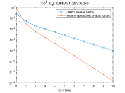
(a) (r05^T, $B_{0}$), the CJ-FEAST GSVDsolver

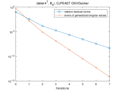
(b) (deter4^T, $B_{0}$), the CJ-FEAST GSVDsolver

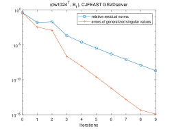
(c) (dw1024^T, $B_{1}$), the CJ-FEAST GSVDsolver

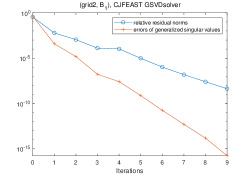
(d) (grid2, $B_{1}$), the CJ-FEAST GSVDsolver

Figure 1: Convergence processes of Ritz approximations.

The figures clearly demonstrate that the selection strategy (33) for the subspace dimension $p$ works well, and the CJ-FEAST GSVDsolver always converges linearly but quite fast. In the meantime, the choral metric errors of Ritz values are approximately the squares of the residual norms, which confirms the a priori bounds in Theorem 4.3.

5.3 General performance of the CJ-FEAST GSVDsolver

We now report numerical results on the test problems in Table 1. It is seen from Table 2 that the numbers $n_{gv}$ of desired GSVD components vary greatly, ranging from no more than ten to nearly four hundreds. Also, the desired generalized singular values are either extreme or interior. Therefore, the degree of difficulty to compute the desired GSVD components varies widely.

For each test matrix, we take the series degree $d$ as (68) using $D=1,2,3$, and select the subspace dimensions $p=\lceil 1.1H_{20}\rceil$ and $\lceil 1.5H_{20}\rceil$, where $H_{20}$ is from Table 2. We then use Algorithm 3 to solve the concerning GSVD problems, record the total NLS($k$) with $k$ iteration numbers required for convergence, and list them in Table 3, where NLS denotes the total number of linear systems (38) that are solved and can be regarded as a measure of overall efficiency. For each problem and the same $p$, we used the same initial $Q^{(0)}$, which was the $Q$-factor of the QR factorization of a matrix generated randomly in a normal distribution. Table 3 lists the results obtained.

$(A,B)$	$p$	NLS($k$)
		$D=1$	$D=2$	$D=3$
(r05T, $B_{0}$)	22	30492(42)	31416(21)	31724(14)
	29	40194(42)	41412(21)	38831(13)
(deter4T, $B_{0}$)	85	142800(16)	125545(7)	108120(4)
	116	133980(11)	122380(5)	110664(3)
(lp_bnl2T, $B_{0}$)	10	2000(4)	3060(3)	3080(2)
	14	2100(3)	4284(3)	4312(2)
(G65, $B_{0}$)	419	5703428(83)	5530800(40)	4977720(24)
	572	938080(10)	755040(4)	1132560(4)
(nopoly, $B_{0}$)	71	796620(33)	726330(15)	654336(9)
	96	163200(5)	196416(3)	294912(3)
(tomographic1, $B_{0}$)	1728	15583104(55)	15629760(28)	13934592(17)
	2356	3541068(10)	3946300(6)	4749696(5)
(denormal, $B_{0}$)	786	6277782(50)	5413968(22)	4649976(13)
	1072	1397888(9)	1406464(5)	1585488(4)
(flower_5_4T, $B_{1}$)	20	375200(14)	429120(8)	402300(5)
	27	108540(3)	217242(3)	217242(2)
(dw1024T, $B_{1}$)	113	467368(88)	461605(43)	452452(28)
	154	101332(14)	87780(6)	88088(4)
(p05T, $B_{1}$)	15	98100(10)	117900(6)	117960(4)
	20	104640(8)	104800(4)	117960(3)
(grid2, $B_{1}$)	108	779220(39)	681156(17)	601560(10)
	147	190365(7)	218148(4)	245637(3)

Table 3: The results of different $d$ and $p$: NLS and the number $k$ of iterations used for convergence

We make some comments on Table 3. (i) For each problem and the same subspace dimension $p$, the bigger is the series degree $d$, the fewer iterations are used. (ii) For each problem and the same series $d$, the bigger is $p$, the fewer iterations are used; for at least half of the test problems, the bigger $p$ can speed up the solver very substantially, as is indicated by NLS’s and $k$’s. (iii) For most of the problems, the NLS($k$) do not change much for the same $p$ and different $d$’s, indicating that, for the same $p>n_{gv}$, the overall efficiency is not sensitive to $d$ and a suitably large $d$ works well. (iv) The bigger $n_{gv}$, the harder it is to solve the problem because of relatively big $p$’s.

6 Conclusions

We have proposed a general projection method for computing a partial GSVD of a large regular matrix pair $(A,B)$, and particularly presented a CJ-FEAST GSVDsolver for the computation of the GSVD components of with the generalized singular values in a given interval. The projection method works on the GSVD problem of $(A,B)$ directly and is mathematically equivalent to the Rayleigh–Ritz projection of the SPD pair $(A^{T}A,H)$ with a given right subspace. The CJ-FEAST GSVDsolver constructs an approximate spectral projector $P$ of $(A^{T}A,H)$ corresponding to the generalized singular values of interest by the CJ series expansion rather than a contour integral-based numerical quadrature or rational filtering that needs to solve several, i.e., $\frac{nnodes}{2}p$, shifted and indefinite large linear systems at each iteration, where the even $nnodes$ is the number of nodes of an underlying numerical quadrature. The CJ-FEAST GSVDsolver exploits subspace iteration on $P$ to generate a sequence of left and right subspaces, projects the concerning GSVD problem of $(A,B)$ directly onto the left and right subspaces, and computes the Ritz approximations to the desired GSVD components.

In terms of the CJ series degree $d$, we have established a reliable estimate for the number $n_{gv}$ of desired GSVD components and the accuracy estimates for the approximate spectral projector $P$ and its eigenvalues. For the CJ-FEAST GSVDsolver, we have established a number of convergence results on the right searching subspace $\mathcal{X}^{(k)}$ and the Ritz approximations. Based on some of the results obtained, we have proposed practical selection strategies for the series degree $d$ and subspace dimension $p$, and developed the CJ-FEAST GSVDsolver.

Illuminating numerical experiments have confirmed our theoretical results and analysis, and demonstrated that the CJ-FEAST GSVDsolver is practical.

References

• [1] F. Alvarruiz, C. Campos, and J. E. Roman, Thick-restarted joint Lanczos bidiagonalization for the GSVD, J. Comput. Appl. Math., (2023), https://doi.org/10.1016/j.cam.2023.115506.
• [2] H. Avron and S. Toledo, Randomized algorithms for estimating the trace of an implicit symmetric positive semi-definite matrix, J. ACM, 58 (2011), pp. Art. 8, 17, https://doi.org/10.1145/1944345.1944349.
• [3] A. k. Björck, Numerical methods for least squares problems, SIAM, Philadelphia, PA, 1996, https://doi.org/10.1137/1.9781611971484.
• [4] A. Cortinovis and D. Kressner, On randomized trace estimates for indefinite matrices with an application to determinants, Found. Comput. Math., 22 (2022), pp. 875–903, https://doi.org/10.1007/s10208-021-09525-9.
• [5] T. A. Davis and Y. Hu, The University of Florida sparse matrix collection, ACM Trans. Math. Software, 38 (2011), pp. Art. 1, 25, https://doi.org/10.1145/2049662.2049663.
• [6] Y. Futamura and T. Sakurai, z-Pares: Parallel Eigenvalue Solver, July 2014, https://zpares.cs.tsukuba.ac.jp/ (accessed 2021-10-19).
• [7] G. H. Golub and C. F. Van Loan, Matrix Computations, Johns Hopkins Studies in the Mathematical Sciences, Johns Hopkins University Press, Baltimore, MD, fourth ed., 2013.
• [8] S. Güttel, E. Polizzi, P. T. P. Tang, and G. Viaud, Zolotarev quadrature rules and load balancing for the FEAST eigensolver, SIAM J. Sci. Comput., 37 (2015), pp. A2100–A2122, https://doi.org/10.1137/140980090.
• [9] P. C. Hansen, Regularization, GSVD and truncated GSVD, BIT, 29 (1989), pp. 491–504, https://doi.org/10.1007/BF02219234.
• [10] P. C. Hansen, Rank-Deficient and Discrete Ill-Posed Problems: Numerical Aspects of Linear Inversion, SIAM, Philadelphia, 1998, https://doi.org/10.1137/1.9780898719697.
• [11] M. E. Hochstenbach, A Jacobi-David type method for the generalized singular value problem, Linear Algebra Appl., 431 (2009), pp. 471–487, https://doi.org/10.1016/j.laa.2009.03.003.
• [12] J. Huang and Z. Jia, On choices of formulations of computing the generalized singular value decomposition of a large matrix pair, Numer. Algorithms, 87 (2021), pp. 689–718, https://doi.org/10.1007/s11075-020-00984-9.
• [13] J. Huang and Z. Jia, Two harmonic Jacobi-Davidson methods for computing a partial generalized singular value decomposition of a large matrix pair, J. Sci. Comput., 93 (2022), https://doi.org/10.1007/s10915-022-01993-7. article no.41.
• [14] J. Huang and Z. Jia, A cross-product free Jacobi-Davidson type method for computing a partial generalized singular value decomposition of a large matrix pair, J. Sci. Comput., 94 (2023), https://doi.org/doi.org/10.1007/s10915-022-02053-w10.1007. article no.3.
• [15] T. Ikegami, T. Sakurai, and U. Nagashima, A filter diagonalization for generalized eigenvalue problems based on the Sakurai-Sugiura projection method, J. Comput. Appl. Math., 233 (2010), pp. 1927–1936, https://doi.org/10.1016/j.cam.2009.09.029.
• [16] A. Imakura, L. Du, and T. Sakurai, A block Arnoldi-type contour integral spectral projection method for solving generalized eigenvalue problems, Appl. Math. Lett., 32 (2014), pp. 22–27, https://doi.org/10.1016/j.aml.2014.02.007.
• [17] A. Imakura, L. Du, and T. Sakurai, Relationships among contour integral-based methods for solving generalized eigenvalue problems, Jpn. J. Ind. Appl. Math., 33 (2016), pp. 721–750, https://doi.org/10.1007/s13160-016-0224-x.
• [18] A. Imakura and T. Sakurai, Complex moment-based method with nonlinear transformation for computing large and sparse interior singular triplets, Sept. 2021, https://doi.org/10.48550/arXiv.2109.13655.
• [19] L. O. Jay, H. Kim, Y. Saad, and J. R. Chelikowsky, Electronic structure calculations for plane-wave codes without diagonalization, Comput. Phys. Commun., 118 (1999), pp. 21–30, https://doi.org/10.1016/S0010-4655(98)00192-1.
• [20] Z. Jia and H. Li, The joint bidiagonalization process with partial reorthogonalization, Numer. Algorithms, 88 (2021), pp. 965–992, https://doi.org/10.1007/s11075-020-01064-8.
• [21] Z. Jia and H. Li, The joint bidiagonalization method for large GSVD computations in finite precision, SIAM J. Matrix Anal. Appl., 44 (2023), pp. 382–407, https://doi.org/10.1137/22M1483608.
• [22] Z. Jia and Y. Yang, A joint bidiagonalization based iterative algorithm for large scale general-form Tikhonov regularization, Appl. Numer. Math., 157 (2020), pp. 159–177, https://doi.org/10.1016/j.apnum.2020.06.001.
• [23] Z. Jia and K. Zhang, An augmented matrix-based CJ-FEAST SVDsolver for computing a partial singular value decomposition with the singular values in a given interval, SIAM J. Matrix Anal. Appl., (2023). accepted.
• [24] Z. Jia and K. Zhang, A FEAST SVDsolver based on Chebyshev–Jackson series for computing partial singular triplets of large matrices, J. Sci. Comput., 97 (2023), https://doi.org/10.1007/s10915-023-02342-y. article no.21.
• [25] J. Kestyn, E. Polizzi, and P. T. P. Tang, FEAST eigensolver for non-Hermitian problems, SIAM J. Sci. Comput., 38 (2016), pp. S772–S799, https://doi.org/10.1137/15M1026572.
• [26] M. E. Kilmer, P. C. Hansen, and M. I. Espanol, A projection-based approach to general-form Tikhonov regularization, SIAM Journal on Scientific Computing, 29 (2007), pp. 315–330.
• [27] K. Kollnig, P. Bientinesi, and E. A. Di Napoli, Rational spectral filters with optimal convergence rate, SIAM J. Sci. Comput., 43 (2021), pp. A2660–A2684, https://doi.org/10.1137/20M1313933.
• [28] C. C. Paige and M. A. Saunders, Towards a generalized singular value decomposition, SIAM J. Numer. Anal., 18 (1981), pp. 398–405, https://doi.org/10.1137/0718026.
• [29] B. N. Parlett, The Symmetric Eigenvalue Problem, vol. 20 of Classics in Applied Mathematics, SIAM, Philadelphia, PA, 1998, https://doi.org/10.1137/1.9781611971163.
• [30] E. Polizzi, Density-matrix-based algorithm for solving eigenvalue problems, Phys. Rev. B, 79 (2009), pp. e115112, 6, https://doi.org/10.1103/PhysRevB.79.115112.
• [31] E. Polizzi, FEAST eigenvalue solver v4.0 user guide, 2020, https://doi.org/10.48550/arXiv.2002.04807.
• [32] T. J. Rivlin, An Introduction to the Approximation of Functions, Dover Books on Advanced Mathematics, Dover Publications, Inc., New York, 1981.
• [33] A. Ruhe, Rational Krylov: a practical algorithm for large sparse nonsymmetric matrix pencils, SIAM J. Sci. Comput., 19 (1998), pp. 1535–1551, https://doi.org/10.1137/S1064827595285597.
• [34] Y. Saad, Iterative Methods for Sparse Linear Systems, SIAM, Philadelphia, PA, second ed., 2003, https://doi.org/10.1137/1.9780898718003.
• [35] Y. Saad, Numerical Methods for Large Eigenvalue Problems, vol. 66 of Classics in Applied Mathematics, SIAM, Philadelphia, PA, 2011, https://doi.org/10.1137/1.9781611970739.
• [36] T. Sakurai and H. Sugiura, A projection method for generalized eigenvalue problems using numerical integration, J. Comput. Appl. Math., 159 (2003), pp. 119–128, https://doi.org/10.1016/S0377-0427(03)00565-X.
• [37] T. Sakurai and H. Tadano, CIRR: a Rayleigh-Ritz type method with contour integral for generalized eigenvalue problems, Hokkaido Math. J., 36 (2007), pp. 745–757, https://doi.org/10.14492/hokmj/1272848031.
• [38] G. W. Stewart, Matrix Algorithms, Vol. I: Basic Decompositions, SIAM, Philadelphia, PA, 1998, https://doi.org/10.1137/1.9781611971408.
• [39] G. W. Stewart, Matrix Algorithms, Vol. II: Eigensystems, SIAM, Philadelphia, PA, 2001, https://doi.org/10.1137/1.9780898718058.
• [40] G. W. Stewart and S. Ji-gunag, Matrix Perturbation Theory, Academic Press, London, 1990.
• [41] P. T. P. Tang and E. Polizzi, FEAST as a subspace iteration eigensolver accelerated by approximate spectral projection, SIAM J. Matrix Anal. Appl., 35 (2014), pp. 354–390, https://doi.org/10.1137/13090866X.
• [42] S. Van Huffel and P. Lemmerling, eds., Total Least Squares and Errors-in-Variables Modeling: Analysis, Algorithms and Applications, Kluwer Academic Publishers, Dordrecht, 2002, https://doi.org/10.1007/978-94-017-3552-0.
• [43] C. F. Van Loan, Generalizing the singular value decomposition, SIAM J. Numer. Anal., 13 (1976), pp. 76–83, https://doi.org/10.1137/0713009.
• [44] H. Zha, Computing the generalized singular values/vectors of large sparse or structured matrix pairs, Numer. Math., 72 (1996), pp. 391–417, https://doi.org/10.1007/s002110050175.