A Stiffness-Oriented Model Order Reduction Method for Low-Inertia Power Systems

Abstract

This paper presents a novel model order reduction technique tailored for power systems with a large share of inverter-based energy resources. Such systems exhibit an increased level of dynamic stiffness compared to traditional power systems, posing challenges for time-domain simulations and control design. Our approach involves rotation of the coordinate system of a linearized system using a transformation matrix derived from the real Jordan canonical form, leading to mode decoupling. The fast modes are then truncated in the rotated coordinate system to obtain a lower-order model with reduced stiffness. Applying the same transformation to the original nonlinear system results in an approximate separation of slow and fast states, which can be truncated to reduce the stiffness. The resulting reduced-order model demonstrates an accurate time-domain performance, the slow eigenvalues of the linearized system are correctly preserved, and a reduction in the model stiffness is achieved, allowing for accurate integration with increased step size. Our methodology is assessed in detail for a 3-bus system with generation units involving grid-forming/following converters and synchronous machines, where it allows for a computational speed-up of up to $\mathbf{100x}$ compared to the original system. Several standard larger test systems are also considered.

Submitted to the 23rd Power Systems Computation Conference (PSCC 2024).
$\star$ Simon Muntwiler and Ognjen Stanojev contributed equally to this paper.
This research was supported by NCCR Automation, a National Centre of Competence in Research, funded by the Swiss National Science Foundation (grant number 51NF40_180545). The work of Simon Muntwiler was supported by the Bosch Research Foundation im Stifterverband.

I Introduction

The increased penetration of inverter-based energy resources in power systems has significantly changed the dynamic characteristics of the system, as the converter dynamics and their controls operate on a timescale that closely aligns with the network dynamics [1]. Consequently, conventional modeling and simulation approaches relying on the assumption of a timescale separation between line and generation dynamics have become inadequate, necessitating the development of novel power system simulation models. One of the challenges in developing new simulation tools lies in determining the appropriate level of the model complexity [2]. Recent studies propose detailed modeling of network dynamics, inverter-based resources, and loads to represent all the relevant dynamic phenomena [3]. Nevertheless, these dynamic models exhibit a significant degree of stiffness and a large number of variables, thus becoming intractable even when being solved with state-of-the-art variable time step integration methods.

Recent literature proposes using model order reduction (MOR) techniques to ensure computational tractability while preserving sufficient modeling detail required to analyze low-inertia systems. A widely used concept in MOR is to formulate a system in singularly perturbed form, where the slow and fast dynamics are separated. The model order and stiffness can then be reduced by treating the fast states as algebraic variables [4, 5, 6, 7, 8, 2, 9]. This concept has been employed for instance for reducing the order of synchronous machine models [4], eliminating fast-varying dynamics of networks of grid-forming inverters [8], constructing a tractable model of low-inertia systems for control design [6]. The main challenge, however, is to transform a system into a singularly perturbed form, especially in the case of nonlinear systems.

Various transformation methods to obtain a system in singularly perturbed form exist such as participation factor analysis [10, 11, 12], modal reduction [13, 14], and balanced truncation [15, 16]. In [10, 11, 12], a separation between fast and slow modes is leveraged based on modal analysis and participation factors [17]. Reduced converter models of single converter units were initially formulated in [10], and subsequently extended in [11] to converter interconnections, through sequential elimination of the fastest modes based on participation factors. Using a similar methodology, [12] proposed an approach to identify the transmission lines most critical for system stability and the necessary level of their model complexity. Although participation factors provide supplementary insights, their interpretability is frequently obscured by the co-participation of multiple states in a single mode. Moreover, the aforementioned methods may not consistently preserve the stability characteristics of the original system, as shown in [2].

The approaches based on modal analysis and PFA reviewed above reduce the order of the system by manipulating the original system states and equations, thereby preserving the physical interpretation of variables. However, methods that perform order reduction in a transformed space, such as balanced truncation and modal reduction, generally achieve models of higher quality [18]. The balanced truncation method possesses theoretical advantages over alternative approaches as a global error bound can be established and stability properties are maintained [19]. However, it requires the calculation of controllability and observability Gramians by solving two dual Lyapunov equations [15], which leads to computational difficulties. While the modal reduction methods [13, 14] are also promising, previous research only focused on conventional and linear power system models.

This paper proposes a novel MOR technique, building upon the traditional modal reduction approaches, directly targeting the reduction of the model stiffness while at the same time preserving the critical eigenvalues of the linearized system. Therefore, small-signal stability properties of the (linearized) original system are preserved, and larger integration step sizes are viable without a significant loss in model accuracy. In the proposed approach, the coordinate system of a linearized system is first rotated using an orthonormal matrix obtained via the real Jordan canonical form, yielding decoupling of the system modes. The fast modes are then truncated in the rotated coordinate system to obtain a lower-order model with lower stiffness, while the slow modes are entirely preserved. Applying the same transformation to the original nonlinear system results in an approximate separation of slow and fast states, which are transformed into algebraic variables to reduce the model order. In contrast to [10, 2] where only single inverter infinite bus system configurations are considered or [11, 6, 8] where interconnections of only grid-forming converters are considered, we investigate realistic generation portfolios in low-inertia systems, including synchronous machines and grid-forming and grid-following converters. We perform a detailed analysis of the effectiveness of the proposed method and compare it to the state-of-the-art methods from the literature using several standard test transmission networks.

II Preliminaries

II-A Considered DAE Systems

We consider stiff dynamical systems which are described by a nonlinear differential-algebraic equation (DAE) of the form

$$\tfrac{\operatorname{d}}{\operatorname{d}\!t}{x} =f(x,u,z),$$ (1a)

$$0 =g(x,u,z),$$ (1b)

where $x\in\mathbb{R}^{n_{\mathrm{x}}}$ are the differential system states, $u\in\mathbb{R}^{n_{\mathrm{u}}}$ the control inputs, and $z\in\mathbb{R}^{n_{\mathrm{z}}}$ algebraic variables. We rely on the following assumption to ensure the system (1) is numerically solvable [21, Sec. VI.1].

Assumption 1.

The DAE (1) is index-1, i.e.,

$$\frac{\partial g(x,u,z)}{\partial z}\Big{|}_{(x,u,z)=(\bar{x},\bar{u},\bar{z})}$$ (2)

is full-rank for any $(\bar{x},\bar{u},\bar{z})$.

Linearizing (1) around a desired operation point ($x_{o}$, $u_{o}$, $z_{o}$) results (locally) in the linear DAE

$$\tfrac{\operatorname{d}}{\operatorname{d}\!t}\delta x =A_{\mathrm{xx}}\delta x+B_{\mathrm{xu}}\delta u+A_{\mathrm{xz}}\delta z+b_{\mathrm{x}},$$ (3a)

$$0 =A_{\mathrm{zx}}\delta x+B_{\mathrm{zu}}\delta u+A_{\mathrm{zz}}\delta z+b_{\mathrm{z}},$$ (3b)

where $\delta x=x-x_{o}$, $\delta u=u-u_{o}$, $\delta z=z-z_{o}$, $A_{\mathrm{xx}}$, $B_{\mathrm{xu}}$, and $A_{\mathrm{xz}}$ are the Jacobians of $f$ w.r.t. $x$, $u$, $z$, respectively, $A_{\mathrm{zx}}$, $B_{\mathrm{zx}}$, and $A_{\mathrm{zz}}$ are the Jacobians of $g$ w.r.t. to $x$, $u$, $z$, respectively, and $b_{\mathrm{x}}$ and $b_{\mathrm{z}}$ are the bias terms. Under Assumption 1, $A_{\mathrm{zz}}$ is regular and (3b) can be rearranged to

$$\delta z=A_{\mathrm{zz}}^{-1}(A_{\mathrm{zx}}\delta x+B_{\mathrm{zu}}\delta u+b_{\mathrm{z}}).$$ (4)

It follows that (3) can be equivalently represented by the linear ODE

$$\tfrac{\operatorname{d}}{\operatorname{d}\!t}\delta x= \underbrace{(A_{\mathrm{xx}}+A_{\mathrm{xz}}A_{\mathrm{zz}}^{-1}A_{\mathrm{zx}})}_{=\vcentcolon\tilde{A}}\delta x+\underbrace{b_{\mathrm{x}}+A_{\mathrm{zz}}^{-1}b_{\mathrm{z}}}_{=\vcentcolon\tilde{b}}$$

$$+\underbrace{(B_{\mathrm{xx}}+A_{\mathrm{xz}}A_{\mathrm{zz}}^{-1}B_{\mathrm{zu}})}_{=\vcentcolon\tilde{B}}\delta u.$$ (5)

The eigenvalues of $\tilde{A}$ are denoted as $\lambda_{i}$ with $i\in\{1,\ldots,n_{\mathrm{x}}\}$ and ordered according to their real part, i.e., $\Re(\lambda_{1})\leq\Re(\lambda_{2})\leq\ldots\leq\Re(\lambda_{n_{\mathrm{x}}})$. The corresponding right and left eigenvectors of $\tilde{A}$ are denoted as $y_{i}$ and $v_{i}$, respectively, for $i\in\{1,\ldots,n_{\mathrm{x}}\}$, and defined by

$$\tilde{A}y_{i} =y_{i}\lambda_{i}, y_{i}\neq 0,$$ (6)

$$v_{i}^{\top}\tilde{A} =\lambda_{i}v_{i}^{\top}, v_{i}\neq 0.$$ (7)

In Section IV, we show how to obtain a DAE (1) for a generic low-inertia power system. Assumption 1 has been proven to hold for a linear power system DAE (3) in [22], whereas a proof for nonlinear DAEs (1) is still an open problem [23].

II-B Definition of Stiffness

Stiffness in linear ODE systems of the form (II-A) is often assessed through the so-called stiffness ratio[24], i.e., the ratio

$$\rho=\frac{|\Re(\lambda_{1})|}{|\Re(\lambda_{n_{\mathrm{x}}})|}.$$ (8)

In particular, a system (II-A) is denoted as stiff if all eigenvalues of $\tilde{A}$ have negative real parts and the stiffness ratio is large [24, Sec. 6.2]. Stiffness of the original system (1) is then assessed through the stiffness ratio of the linearized system (II-A).

In more general terms, a system is considered as stiff if implicit integration methods work significantly better compared to explicit ones [21, Chap. IV]. Consequently, accurate integration of a stiff system (1) using an explicit method requires extremely small step sizes [24, Sec. 6]. Thus, simulations of (1) are computationally expensive and it is in general intractable to use the model for control or estimation purposes. The objective of this paper is to obtain a stiffness-oriented MOR that allows for accurate integration of (1) using comparably large step sizes.

III Model Order Reduction

A common approach to reduce the order and associated stiffness of a model is the concept of singular perturbation [2, 9, 4, 5, 6, 7, 8]. Assume (1) can be transformed to the singularly perturbed DAE

$$\tfrac{\operatorname{d}}{\operatorname{d}\!t}\delta x_{\mathrm{s}} =f_{\mathrm{s}}(x_{\mathrm{s}},x_{\mathrm{f}},u,z),$$ (9a)

$$\epsilon\cdot\tfrac{\operatorname{d}}{\operatorname{d}\!t}\delta x_{\mathrm{f}} =f_{\mathrm{f}}(x_{\mathrm{s}},x_{\mathrm{f}},u,z)$$ (9b)

$$0 =g(x_{\mathrm{s}},x_{\mathrm{f}},u,z),$$ (9c)

where $x_{\mathrm{s}}$ and $x_{\mathrm{f}}$ represent slow and fast states, respectively, and $\epsilon\in\mathbb{R}_{\geq 0}$ is a small positive scalar. Additionally, assuming that $\frac{\partial f_{\mathrm{f}}}{\partial x_{\mathrm{f}}}$ is Hurwitz stable, model order reduction can be performed by setting $\epsilon=0$ leading to the reduced-order DAE

$$\tfrac{\operatorname{d}}{\operatorname{d}\!t}\delta x_{\mathrm{s}} =f_{\mathrm{s}}(x_{\mathrm{s}},x_{\mathrm{f}},u,z),$$ (10a)

$$0 =f_{\mathrm{f}}(x_{\mathrm{s}},x_{\mathrm{f}},u,z)$$ (10b)

$$0 =g(x_{\mathrm{s}},x_{\mathrm{f}},u,z),$$ (10c)

with reduced stiffness. As shown in [25, Thm. 6.2], the solution to the DAE (10a)-(10b) recovers the solution to the original ODE (9a)-(9b) for $\epsilon\rightarrow 0$. However, transforming the original system (1) to singularly perturbed form (9) is in general challenging. In the following, we describe two methods to achieve this transformation: A classical one based on PFA (Section III-A) and our proposed stiffness-oriented MOR (Section III-B).

III-A Participation factor analysis

Participation factor analysis (PFA) [17] is a tool to analyze the contribution of the states of a linear system (II-A) to its modes. The corresponding participation matrix $P\in\mathbb{R}^{n\times n}$ associated to $\tilde{A}$ in (II-A) can be obtained as

$$P_{ki}=[v_{i}]_{k}[y_{i}]_{k},$$ (11)

where $[v]_{k}$ denotes the $k^{\mathrm{th}}$ entry of vector $v$. The solution of the autonomous and unbiased system (II-A) (i.e., (II-A) with $\delta u=0$ and $\tilde{b}=0$) can be obtained as

$$x(t)=\sum_{i=1}^{n}v_{i}^{\top}x(0)e^{\lambda_{i}t}y_{i}$$ (12)

and, if $x(0)=y_{i}$,

$$x(t)=v_{i}^{\top}y_{i}y_{i}e^{\lambda_{i}t}=\sum_{k=1}^{n}(P_{ki})y_{i}e^{\lambda_{i}t}.$$ (13)

Consequently, the participation factor $P_{ki}$ measures the relative contribution of the $k^{\mathrm{th}}$ state in the time response associated with the $i^{\mathrm{th}}$ mode. Thus, the participation matrix $P$ can be used to identify the states that contribute to the fast modes. Thus, (II-A) is transformed to singularly perturbed form by introducing slow and fast states as $x_{\mathrm{s}}=T_{\mathrm{s}}^{\mathrm{pfa}}x$ and $x_{\mathrm{f}}=T_{\mathrm{f}}^{\mathrm{pfa}}x$, respectively, where $T_{\mathrm{s}}^{\mathrm{pfa}}$ is an identity matrix with zeros on its diagonal at entries corresponding to states with large contribution to fast modes and $T_{\mathrm{f}}^{\mathrm{pfa}}=I-T_{\mathrm{s}}^{\mathrm{pfa}}$. The original system (1) can be transformed into singularly perturbed form (approximately) with $f_{\mathrm{s}}(x_{\mathrm{s}},x_{\mathrm{f}},u,z)=T_{\mathrm{s}}^{\mathrm{pfa}}f(x,u,z)$ and $f_{\mathrm{f}}(x_{\mathrm{s}},x_{\mathrm{f}},u,z)=T_{\mathrm{f}}^{\mathrm{pfa}}f(x,u,z)$. While this allows us to reduce the model order, the approach might fail at significantly reducing the stiffness and preserving the original dynamics due to the non-negligible coupling between slow and fast modes. We will demonstrate this in the numerical example in Section V below.

III-B Proposed stiffness-oriented model order reduction

To overcome the limitations of classical MOR using PFA, we propose a stiffness-oriented MOR technique. The underlying idea is to perform PFA on system (II-A) in a rotated coordinate system where slow and fast modes are completely decoupled. Since $\tilde{A}$ is a real square matrix, we can obtain the real Jordan canonical form $\tilde{A}=TJT^{-1}$ with real transformation matrix $T$ obtained as

$$T= \begin{bmatrix}T_{1},T_{2},\ldots,T_{n_{\mathrm{x}}}\end{bmatrix},$$

$$T_{i}= \frac{\tilde{T}_{i}}{\|\tilde{T}_{i}\|_{2}}\text{ with }\tilde{T}_{i}=\begin{cases}y_{i}&\text{if }\lambda_{i}\text{ is real},\\ \Re(y_{i})&\text{if }\lambda_{i}\text{ is complex},\\ \Im(y_{i})&\text{if }T_{i-1}=\Re(y_{i-1}),\end{cases}$$

and real block-diagonal Jordan matrix $J=T^{-1}\tilde{A}T$ [26, Sec. 3.4]. This allows us to transform (II-A) to

$$\tfrac{\operatorname{d}}{\operatorname{d}\!t}\delta\tilde{x}=J\delta\tilde{x}+T^{-1}\tilde{B}\delta u+T^{-1}\tilde{b},$$ (14)

with state $\delta\tilde{x}=\tilde{x}-\tilde{x}_{o}=T^{-1}x$ and $\tilde{x}_{o}=T^{-1}x_{o}$. The resulting system is block-diagonal with each block being associated with a pair of conjugate eigenvalues. Consequently, the modes in (14) are completely decoupled and the PFA matrix $P$ is block-diagonal. We can extract the states associated with the $n_{\mathrm{s}}\in[0,n_{\mathrm{x}}]$ slowest and $n_{\mathrm{f}}=n_{\mathrm{x}}-n_{\mathrm{s}}$ fastest modes as $\tilde{x}_{\mathrm{s}}=T_{\mathrm{s}}\tilde{x}$ and $\tilde{x}_{\mathrm{f}}=T_{\mathrm{f}}\tilde{x}$, respectively, with $T_{\mathrm{s}}=\begin{bmatrix}0&I_{n_{\mathrm{s}}}\end{bmatrix}$ and $T_{\mathrm{f}}=\begin{bmatrix}I_{n_{\mathrm{f}}}&0\end{bmatrix}$. Herein, deciding on the number of slow states $n_{\mathrm{s}}$ is a choice of the user and subject to the trade-off between reduced stiffness and lower accuracy of the resulting reduced model w.r.t. to the original model, compare our numerical examples in Section V below. Thus, the system (14) can easily be brought into singularly perturbed form (9).

An (approximate) separation of slow and fast modes in the original (nonlinear) DAE (1) can be obtained as

$$\tfrac{\operatorname{d}}{\operatorname{d}\!t}\tilde{x}_{\mathrm{s}} =T_{\mathrm{s}}T^{-1}f(T\tilde{x},u,z),$$ (15a)

$$\tfrac{\operatorname{d}}{\operatorname{d}\!t}\tilde{x}_{\mathrm{f}} =T_{\mathrm{f}}T^{-1}f(T\tilde{x},u,z),$$ (15b)

$$0 =g(T\tilde{x},u,z).$$ (15c)

Finally, MOR can be performed by applying the concept of singular perturbation to (15) by treating the fast modes as algebraic variables, i.e., setting $\tfrac{\operatorname{d}}{\operatorname{d}\!t}\tilde{x}_{\mathrm{f}}=0$ in (15c). This results in a model with reduced stiffness which accurately captures the slow dynamics of the original system as can be seen in the numerical examples provided in Section V. In contrast to the proposed method, applying PFA to the original system (1) may fail at reducing the stiffness of the system. However, note that the states in the reduced-order system (15) loose their physical meaning. A similar MOR approach was used in [27], where a linear system (II-A) was transformed to a balanced system with states ordered according to their controllability. The nonlinear ODE is then transformed to a similar form as (15), where the reduced states are either completely neglected [28] or approximated using linear dynamics [16]. In contrast, relying on the real Jordan canonical form allows us to decouple slow and fast states in the linear system (14) and therefore effectively reduce the stiffness in (15).

IV Modeling and Control of Low-Inertia Systems

While the MOR technique introduced in Section III-B is applicable to any stiff DAE system of the form (1), the focus of this work is on low-inertia power systems. This section overviews the typical components of these systems, including synchronous machines and grid-forming/following converters. Additionally, dynamics of transmission lines are also included due to their effect on the stability of the system [3]. The modeling and control are implemented in a Synchronously-rotating Reference Frame (SRF) and a per-unit system.

IV-A Graph-theoretic Network Modeling & Line Dynamics

We consider a transmission power network represented by a connected graph $\mathcal{G}(\mathcal{N},\mathcal{E})$, with $\mathcal{N}\coloneqq\{1,\dots,n\}$ denoting the set of network nodes, and $\mathcal{E}\subseteq\mathcal{N}\times\mathcal{N}$ representing the set of network branches. The node set is partitioned as $\mathcal{N}=\mathcal{N}_{\mathrm{sg}}\cup\mathcal{N}_{\mathrm{gfm}}\cup\mathcal{N}_{\mathrm{gfl}}\cup\mathcal{N}_{\mathrm{load}}$ to define sets of nodes hosting synchronous generators, grid-forming, grid-following converters, and loads. For every bus $i\in\mathcal{N}$, let $v_{i}\in\mathbb{R}^{2}$ denote the associated voltage vector (comprised of a $d$ and a $q$ component). For each line $(i,j)\in\mathcal{E}$, let $r_{ij}\in\mathbb{R}_{\geq 0}$ and $l_{ij}\in\mathbb{R}_{\geq 0}$ denote its respective resistance and inductance values, and $i_{ij}\in\mathbb{R}^{2}$ represent the corresponding branch current. The transmission grid is modeled by the following differential equation, written in a dq-frame rotating at frequency $\omega_{g}$ as:

$$\tfrac{\operatorname{d}}{\operatorname{d}\!t}{i}_{ij}=\frac{\omega_{b}}{\ell_{ij}}(v_{i}-v_{j})-\left(\frac{r_{ij}}{\ell_{ij}}\omega_{b}+\mathcal{J}\omega_{b}\omega_{g}\right)i_{ij},\forall(i,j)\in\mathcal{E}$$ (16)

with $w_{b}$ representing the base frequency, and $\mathcal{J}$ denoting the $2\times 2$, 90-degree rotation matrix.

IV-B Power Converter Models

The considered converter model (presented in Fig. 1) consists of a two-level control structure, a switching unit with a constant DC-input voltage, and an AC subsystem, including an RLC filter $(r_{f},c_{f},\ell_{f})$ and a transformer equivalent $(r_{t},\ell_{t})$. In the considered control structure, an outer system-level control layer provides a reference for the converter’s output voltage $v_{f}^{\star}$ that is subsequently tracked by a device-level controller through direct adjustment of the switching voltage $v_{\mathrm{sw}}\coloneqq v_{\mathrm{sw}}^{\star}$.

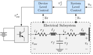
Figure 1: General converter configuration scheme.

IV-B1 System-level Control

The input measurements of the system-level controller are the filter voltage $v_{f}\in\mathbb{R}^{2}$ and the converter current injection into the system $i_{g}\in\mathbb{R}^{2}$, collected in $y_{s}=(v_{f},i_{g})\in\mathbb{R}^{4}$. Using these measurements, we calculate the instantaneous active $p_{c}\coloneqq v^{\mathsf{T}}_{f}i_{g}$ and reactive $q_{c}\coloneqq v^{\mathsf{T}}_{f}\mathcal{J}^{\mathsf{T}}i_{g}$ power. The voltage phasor reference is generated by adjusting the predefined active and reactive setpoints $(p^{\star}_{c},q^{\star}_{c})\in\mathbb{R}^{2}$ according to a measured power imbalance:

$$\omega_{c} =\omega_{s}+\tilde{\omega}_{c},\quad\tfrac{\operatorname{d}}{\operatorname{d}\!t}{\tilde{\omega}}_{c}=-\omega_{z}\tilde{\omega}_{c}+R_{c}^{p}\omega_{z}(p_{c}^{\star}-p_{c}),$$ (17a)

$$v_{c}^{d} =V_{c}^{\star}+\tilde{v}_{c},\quad\tfrac{\operatorname{d}}{\operatorname{d}\!t}{\tilde{v}}_{c}=-\omega_{z}\tilde{v}_{c}+R_{c}^{q}\omega_{z}(q_{c}^{\star}-q_{c}),$$ (17b)

with $R_{c}^{p}\in\mathbb{R}_{>0}$ and $R_{c}^{q}\in\mathbb{R}_{\geq 0}$ are the droop gains, $\omega_{s}$ the synchronization frequency, $\omega_{z}\in\mathbb{R}_{>0}$ denoting the low-pass filter cut-off frequency, $\tfrac{\operatorname{d}}{\operatorname{d}\!t}{\theta}_{c}=\omega_{b}\omega_{c}$ and $v_{c}^{q}=0$. As an additional degree of freedom for stabilization and disturbance rejection, virtual impedance $(r_{v},\ell_{v})\in\mathbb{R}^{2}_{\geq 0}$ of the following form $v_{f}^{\star}=v_{c}-r_{v}i_{g}-\mathcal{J}\omega_{c}\ell_{v}i_{g}$ is commonly implemented.

Grid-Following Mode: A key component of grid-following converters is a synchronization device, commonly a Phase Locked Loop (PLL), which estimates the phase angle $\theta_{s}\in[-\pi,\pi)$ of the voltage $v_{f}$ and the grid frequency $\omega_{s}\in\mathbb{R}_{>0}$:

$$\omega_{s}=\omega_{g}+K_{P}^{s}v_{f}^{q}+K_{I}^{s}\varepsilon,\quad\tfrac{\operatorname{d}}{\operatorname{d}\!t}{\varepsilon}=v_{f}^{q},\quad\tfrac{\operatorname{d}}{\operatorname{d}\!t}{\theta}_{s}=\omega_{b}\omega_{s},$$ (18)

where $(K_{P}^{s},K_{I}^{s})$ are the proportional and integral control gains of the synchronization unit, and $\varepsilon\in\mathbb{R}$ is the integrator state. Therefore, the synchronization frequency $\omega_{s}$ in (17) is for grid-following converters defined by the PLL dynamics (18).

Grid-Forming Mode: In contrast to the grid-following mode of operation, the synchronization unit is not needed for grid-forming control as $\omega_{s}=\omega_{c}^{\star}$ is set to a constant reference. In this way, these units self-synchronize to the power grid by determining the converter frequency and voltage depending on the output power deviations and without the need for PLL.

IV-B2 Device-Level Control

Given a voltage reference $v^{\star}_{f}\in\mathbb{R}^{2}$ in $dq$-coordinates defined by $(\theta_{c},\omega_{c})$, the device-level control is described by a cascade of voltage and current controllers computing a switching voltage reference $v_{\mathrm{sw}}^{\star}\in\mathbb{R}^{2}$:

$$\tfrac{\operatorname{d}}{\operatorname{d}\!t}{\xi} =v^{\star}_{f}-v_{f},$$ (19a)

$$i_{f}^{\star} =K_{P}^{v}(v^{\star}_{f}-v_{f})+K_{I}^{v}\xi+K_{F}^{v}i_{g}+\mathcal{J}\omega_{c}c_{f}v_{f},$$ (19b)

providing an internal current reference $$i_{f}^{\star}$$ followed by

$$\tfrac{\operatorname{d}}{\operatorname{d}\!t}{\gamma} =i_{f}^{\star}-i_{f},$$ (19c)

$$v_{\mathrm{sw}}^{\star} =K_{P}^{i}(i_{f}^{\star}-i_{f})+K_{I}^{i}\gamma+K_{F}^{i}v_{f}+\mathcal{J}\omega_{c}\ell_{f}i_{f},$$ (19d)

where $(K_{P}^{v},K_{P}^{i})\in\mathbb{R}^{2}_{>0}$, $(K_{I}^{v},K_{I}^{i})\in\mathbb{R}^{2}_{\geq 0}$ and $(K_{F}^{v},K_{F}^{i})\in\mathbb{Z}_{\{0,1\}}^{2}$ are the respective proportional, integral, and feed-forward gains, $\xi\in\mathbb{R}^{2}$ and $\gamma\in\mathbb{R}^{2}$ represent the integrator states, and $v$ and $i$ indicate the voltage and current controllers.

IV-C Synchronous Generator Model

We consider a detailed 14th-order model for synchronous generators, including transients in the rotor circuit, swing equation dynamics, a round rotor model equipped with a prime mover and a TGOV1 governor, an AVR based on a simplified excitation system SEXS together with a PSS1A power system stabilizer. Similarly to the converters, the synchronous generator is interfaced to the grid through a transformer and modeled in an SRF. ENTSO-E reference [29] provides more information on the control configuration and tuning parameters, and [30] is suggested for a deeper understanding of the related theory.

IV-D Complete Model

Collecting the algebraic and differential states of the considered units (17)-(19) and network equations (16) in vectors $x$ and $z$, as well as their respective inputs in $u$, we obtain a system of the form given in (1). In the considered system, the fastest dynamics correspond to network dynamics and device-level controllers, with time constants ranging from 1 to 30 ms. On the other hand, the slowest dynamics are related to the mechanical subsystem of synchronous machines with time constants of approx. 10s. Therefore, a stiff DAE can be expected, as confirmed by the case studies presented in the following.

V Numerical Results

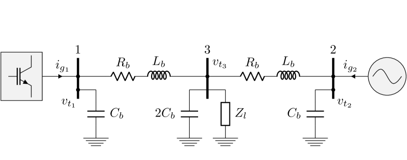
Figure 2: Single line diagram of the considered 3-bus system.

V-A Reducing the Model Order of a 3-bus Low-Inertia System

To numerically evaluate the proposed MOR approach, we first consider the simple 3-bus network ($\mathcal{N}=\{1,2,3\},\mathcal{E}=\{(1,3),(2,3)\}$) depicted in Fig. 2, where two generators are supplying a constant impedance load via long-distance transmission lines. To test the approach on different combinations of generators with diverse characteristics in low-inertia systems, we investigate interactions of all three unit types introduced in Sec. IV:

• Scenario 1: A grid-forming converter and a synchronous generator ($\mathcal{N}_{\mathrm{gfm}}=\{1\},\mathcal{N}_{\mathrm{gfl}}=\emptyset,\mathcal{N}_{\mathrm{sg}}=\{2\}$).

• Scenario 2: A grid-forming and a grid-following converter ($\mathcal{N}_{\mathrm{gfm}}=\{1\},\mathcal{N}_{\mathrm{gfl}}=\{2\},\mathcal{N}_{\mathrm{sg}}=\emptyset$).

• Scenario 3: A synchronous generator and a grid-following converter ($\mathcal{N}_{\mathrm{gfm}}=\emptyset,\mathcal{N}_{\mathrm{gfl}}=\{1\},\mathcal{N}_{\mathrm{sg}}=\{2\}$).

In all three scenarios, the load is set to consume 1 p.u. of active power at nominal voltage, the line parameters are $r_{ij}=0.0146\,\mathrm{p.u.},\ell_{ij}=0.146\,\mathrm{p.u.},\forall(i,j)\in\mathcal{E}$, and the generators are set to share the load equally. Converter parameters are adopted from [3, Table 1] and synchronous machine parameters from [3, Table 2]. The considered test system configurations are implemented in MATLAB using CasADi [31] for symbolic modeling. We mainly employ Acados [32] for numerical integration and occasionally resort to MATLAB’s ode15s variable time-step solver for benchmarking purposes.

TABLE I: Participation Factor Analysis of the 3-bus System.

Configuration	$\boldsymbol{\rho}$	Fastest Modes	States	PF
Scenario 1	5.4E4	$-4565\pm\mathrm{j}478$	$i_{g},i_{13}$	$0.75$
		$-2252\pm\mathrm{j}689$	$v_{f},i_{23}$	$0.88$
		$-1271\pm\mathrm{j}3785$	$v_{f}$	$0.67$
		$-1181\pm\mathrm{j}3787$	$v_{f},i_{g}$	$0.86$
Scenario 2	3.0E4	$-4678\pm\mathrm{j}356$	$i_{g},i_{13},i_{23}$	$0.99$
		$-3641\pm\mathrm{j}231$	$i_{g}$	$0.6$
		$-1953\pm\mathrm{j}3995$	$v_{f}$	$0.66$
		$-1887\pm\mathrm{j}3720$	$v_{f}$	$0.64$
		$-841\pm\mathrm{j}0$	$v_{f},i_{23}$	$0.78$
		$-799\pm\mathrm{j}0$	$v_{f}$	$0.64$
		$-698\pm\mathrm{j}4131$	$v_{f},\tilde{\omega}_{c}$	$0.66$
		$-667\pm\mathrm{j}3954$	$v_{f},\tilde{\omega}_{c}$	$0.64$
Scenario 3	4.4E4	$-4554\pm\mathrm{j}451$	$i_{g},i_{13},i_{23}$	$0.98$
		$-2286\pm\mathrm{j}456$	$v_{f},i_{13}$	$0.85$
		$-1293\pm\mathrm{j}3946$	$v_{f},i_{g}$	$0.85$
		$-1160\pm\mathrm{j}3698$	$v_{f},i_{g},i_{23}$	$0.95$

The proposed approach is evaluated against a standard method in the literature [2, 10, 11, 12], where the states to be removed are selected based on their participation in the fastest modes, as discussed in Sec. III-A. Table I showcases the stiffness ratio and the fastest modes for each considered scenario, and details the states with the highest participation factors in these modes. As can be seen from Table I, all three scenarios are characterized by a high stiffness ratio. To perform PFA-based model reduction, we residualize the states indicated in the table for each respective scenario. As expected, the states to be removed are related to the electrical variables of the converter and the network. On the other hand, the fast modes indicated in Table I are removed in the proposed stiffness-oriented MOR after rotating the original state space, as discussed in (14). Therefore, in Scenario 1 and 3, the number of eliminated modes is 8, while in Scenario 2 it is 14.

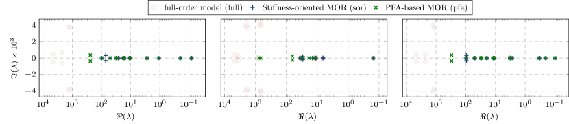
Figure 3: Eigenvalue spectrum of full and reduced models for Scenario 1 (left), Scenario 2 (mid), and Scenario 3 (right).

V-B Modal Analysis

In Fig. 3, we present eigenvalue spectrum plots for the original system model ($\mathrm{full}$), the model reduced through PFA ($\mathrm{pfa}$), and the model reduced using the proposed stiffness-oriented MOR ($\mathrm{sor}$) across the three considered scenarios. Our findings indicate that the proposed method effectively preserves the slowest modes while significantly reducing stiffness. More precisely, the new stiffness ratios of the three scenarios are respectively $\rho_{1}^{\mathrm{sor}}=1.1\mathrm{E}3,\rho_{2}^{\mathrm{sor}}=2.4\mathrm{E}2,\rho_{3}^{\mathrm{sor}}=9.3\mathrm{E}2$. On the other hand, the PFA-based approach clearly modifies certain modes. The stiffness ratios of the PFA reduced models are $\rho_{1}^{\mathrm{pfa}}=5.2\mathrm{E}3,\rho_{2}^{\mathrm{pfa}}=5\mathrm{E}3,\rho_{3}^{\mathrm{pfa}}=4.5\mathrm{E}3$. Finally, it is worth noting that for lower-order models PFA-based reduction results in significant modifications of the critical eigenvalues, as also found in [2].

V-C Accuracy of the Reduced Order Models

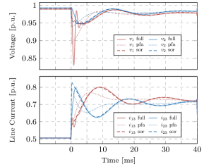
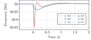
Figure 4: Time domain solution of distinct slow and fast states for Scenario 1.

In Fig. 4, we show the time domain evolution of selected fast modes (voltages and line currents) and slow modes (frequencies) of the considered 3-bus system in Scenario 1 after a 30% load drop at time $t=0$. The integration is performed using acados with implicit Runge-Kutta (Gauss-Legendre of order $4$) and a (small) step size of $h=2.5E-4$ for all three models, i.e., $\mathrm{full}$, $\mathrm{sor}$, and $\mathrm{pfa}$. It can be seen that all models capture the slow dynamics very accurately. However, the PFA-based approach leads to large integration errors for the fast states, while the model based on the proposed reduction technique is significantly more accurate. Interestingly, the very fast voltage dynamics appear to be averaged immediately following the load loss.

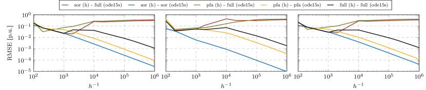
Figure 5: RMSE vs. inverse of step size ($h^{-1}$) for different combinations of models (the reduced model obtained using the proposed stiffness-oriented MOR ($\mathrm{sor}$), the reduced model using PFA ($\mathrm{pfa}$) and the original full model ($\mathrm{full}$) for Scenario 1 (left), Scenario 2 (mid), and Scenario 3 (right).

To assess the model accuracy in more detail across all considered scenarios and to quantify the computational benefit resulting from the presented reduced order models, we evaluate the discrepancy between two models ($\mathrm{mod1}$ and $\mathrm{mod2}$) within the time span $t\in[0,T_{\mathrm{end}}]$ with end time $T_{\mathrm{end}}=0.1s$ through the normalized root mean square error (RMSE), calculated as

$$\mathrm{RMSE}(h)=\sqrt{\frac{h}{T_{\mathrm{end}}}\sum_{i=1}^{T_{\mathrm{end}}\cdot h^{-1}}\frac{\|x_{\mathrm{mod}1}^{h}(i\cdot h)-x_{\mathrm{mod}2}^{\mathrm{ode15s}}(i\cdot h)\|_{2}^{2}}{\|x_{\mathrm{mod}2}^{\mathrm{ode15s}}(i\cdot h)\|_{2}^{2}}},$$

where $x_{\mathrm{mod}1}^{h}(t)$ is obtained by integration of $\mathrm{mod1}$ with fixed time step $h$ and $x_{\mathrm{mod}2}^{\mathrm{ode15s}}(t)$ by integration of $\mathrm{mod}2$ using the computationally expensive but very accurate solver ode15s.

In Fig. 5, we show the RMSE w.r.t. to the inverse step size $h^{-1}$ of the integrator for all three scenarios and different model combinations. Examining the blue, yellow, and black curves which show the RMSE error of all models ($\mathrm{sor/pfa/full}$) when integrated with the fixed step size $h$ and ode15s, it becomes clear that $\mathrm{sor}$ results in the same RMSE with up to $10\mathrm{x}/100\mathrm{x}$ larger step size compared to $\mathrm{pfa/full}$. This result highlights the computational benefit of the proposed approach which is especially promising for step size control [21, Chap. IV]. Step size control is applied in variable time step solvers that reduce the step size in an adaptive manner during integration whenever the error relative to the exact solution is above a certain threshold.

Additionally, by examining the red and green curves which show the RMSE of $\mathrm{sor/pfa}$ integrated with step size $h$ and the full-order model integrated with ode15s, we can see that the proposed approach more accurately captures the model dynamics. The exceptions, mainly in Scenario 2, where $\mathrm{pfa}$ is more accurate for specific step sizes, arise as $\mathrm{pfa}$ captures more accurately very fast changes in states (e.g., voltage dips), as can also be observed in Fig. 4 around $t=0$. Thereby, Scenario 2 highlights the trade-off between a reduction in computational cost and resulting accuracy compared to the full model.

TABLE II: Performance of MOR on larger test cases.

Test Case	# Fast Modes	$\boldsymbol{\rho}$			RMSE
		orig	sor	pfa	sor	pfa
9-bus IEEE	18	4E5	9E2	1E4	0.1097	0.1439
3AreaKundur	40	2E11	8E2	5E3	0.5292	0.6303
39-bus IEEE	104	6E11	2E2	6E2	0.2524	0.3172

V-D Reducing the Model of Larger-scale Low-Inertia Systems

After acquiring a fundamental understanding of the considered MOR techniques in a simplified low-inertia test environment, we expand our analysis to larger test cases. Specifically, we examine a 9-bus system, which includes one generator of each type, totaling three generators, a 3-area test system with two units of the same type in each area, and a modified IEEE 39-bus system with three grid-forming units and seven synchronous machines. The results in Table II demonstrate that the benefits of the proposed MOR scheme extend to larger test cases. In particular, the proposed approach consistently outperforms the PFA approach in both the model accuracy and the reduction of the model stiffness, indicating the possibility of using larger integration steps. The RMSE is computed following the same procedure as in the previous subsection, with the integration step of $h=1\mathrm{E}-5$.

VI Conclusions

In this paper, we proposed a stiffness-oriented model order reduction (MOR) approach which was shown to effectively reduce the stiffness of low inertia power system models. Consequently, an up to 100 times speed-up of the integration compared to the original (stiff) model allows us to drastically reduce the computational cost while maintaining accurate integration. The resulting reduced order modelling is especially promising for optimization-based estimation and control, which we intend to investigate in future work.

References

- [1] F. Dörfler and D. Groß, “Control of low-inertia power systems,” Annual Review of Control, Robotics, and Autonomous Systems, vol. 6, no. 1, pp. 415–445, 2023.
- [2] I. Caduff, U. Markovic, C. Roberts, G. Hug, and E. Vrettos, “Reduced-order modeling of inverter-based generation using hybrid singular perturbation,” Electric Power Systems Research, vol. 190, p. 106773, 2021.
- [3] U. Markovic, O. Stanojev, P. Aristidou, E. Vrettos, D. Callaway, and G. Hug, “Understanding small-signal stability of low-inertia systems,” IEEE Trans. Power Syst., vol. 36, no. 5, pp. 3997–4017, 2021.
- [4] S. Ahmed-Zaid, P. Sauer, M. Pai, and M. Sarioglu, “Reduced order modeling of synchronous machines using singular perturbation,” IEEE Trans. on Circuits and Systems, vol. 29, no. 11, pp. 782–786, 1982.
- [5] L. Luo and S. V. Dhople, “Spatiotemporal model reduction of inverter-based islanded microgrids,” IEEE Trans. on Energy Conversion, vol. 29, no. 4, pp. 823–832, 2014.
- [6] S. Curi, D. Groß, and F. Dörfler, “Control of low-inertia power grids: A model reduction approach,” in Proc. CDC, 2017, pp. 5708–5713.
- [7] P. Vorobev, P.-H. Huang, M. Al Hosani, J. L. Kirtley, and K. Turitsyn, “High-fidelity model order reduction for microgrids stability assessment,” IEEE Trans. Power Syst., vol. 33, no. 1, pp. 874–887, 2018.
- [8] O. Ajala, N. Baeckeland, B. Johnson, S. Dhople, and A. Domínguez-García, “Model reduction and dynamic aggregation of grid-forming inverter networks,” IEEE Trans. Power Syst.s, pp. 1–16, 2022.
- [9] P. Kokotović, H. K. Khalil, and J. O’reilly, Singular perturbation methods in control: analysis and design. SIAM, 1999.
- [10] Q. Cossart, F. Colas, and X. Kestelyn, “Model reduction of converters for the analysis of 100% power electronics transmission systems,” in Proc. ICIT, 2018, pp. 1254–1259.
- [11] ——, “A novel event- and non-projection-based approximation technique by state residualization for the model order reduction of power systems with a high renewable energies penetration,” IEEE Trans. Power Syst., vol. 37, no. 4, pp. 3221–3229, 2022.
- [12] G. Grdenić, M. Delimar, and J. Beerten, “AC grid model order reduction based on interaction modes identification in converter-based power systems,” IEEE Trans. Power Syst., vol. 38, no. 3, pp. 2388–2397, 2023.
- [13] W. W. Price et al., “Testing of the modal dynamic equivalents technique,” IEEE Trans. on Power Apparatus and Systems, vol. PAS-97, no. 4, pp. 1366–1372, 1978.
- [14] S. de Oliveira and J. de Queiroz, “Modal dynamic equivalent for electric power systems. i. theory,” IEEE Trans. Power Syst., vol. 3, no. 4, pp. 1723–1730, 1988.
- [15] F. D. Freitas, J. Rommes, and N. Martins, “Gramian-based reduction method applied to large sparse power system descriptor models,” IEEE Trans. Power Syst., vol. 23, no. 3, pp. 1258–1270, 2008.
- [16] D. Osipov and K. Sun, “Adaptive nonlinear model reduction for fast power system simulation,” IEEE Trans. Power Syst., vol. 33, no. 6, pp. 6746–6754, 11 2018.
- [17] I. J. Perez-Arriaga, G. C. Verghese, and F. C. Schweppe, “Selective modal analysis with applications to electric power systems, Part I: Heuristic introduction,” IEEE Trans. on Power Apparatus and Systems, vol. PAS-101, no. 9, pp. 3117–3125, 1982.
- [18] Z. Zhu, G. Geng, and Q. Jiang, “Power system dynamic model reduction based on extended Krylov subspace method,” IEEE Trans. Power Syst., vol. 31, no. 6, pp. 4483–4494, 2016.
- [19] A. Antoulas, “Approximation of large-scale dynamical systems: An overview,” IFAC Proceedings Volumes, vol. 37, no. 11, pp. 19–28, 2004.
- [20] S. Reich, “On an existence and uniqueness theory for nonlinear differential-algebraic equations,” Circuits, Systems and Signal Processing, vol. 10, pp. 343–359, 1991.
- [21] E. Hairer and G. Wanner, Solving ordinary differential equations II. Springer Berlin Heidelberg New York, 1996, vol. 375.
- [22] S. A. Nugroho, A. F. Taha, N. Gatsis, and J. Zhao, “Observers for differential algebraic equation models of power networks: Jointly estimating dynamic and algebraic states,” IEEE Trans. on Control of Network Systems, vol. 9, no. 3, pp. 1531–1543, 2022.
- [23] T. Groß, S. Trenn, and A. Wirsen, “Solvability and stability of a power system dae model,” Systems & Control Letters, vol. 97, pp. 12–17, 2016.
- [24] J. D. Lambert, Numerical methods for ordinary differential systems. Wiley New York, 1991, vol. 146.
- [25] R. E. O’Malley Jr, “Topics in singular perturbations,” Advances in Mathematics, vol. 2, no. 4, pp. 365–470, 1968.
- [26] R. A. Horn and C. R. Johnson, Matrix analysis. Cambridge University Press, 2012.
- [27] X. Ma and J. A. De Abreu-Garcia, “On the computation of reduced order models of nonlinear systems using balancing technique,” Proc. CDC, pp. 1165–1166, 1988.
- [28] A. Verhoeven, J. Ter Maten, M. Striebel, and R. Mattheij, “Model order reduction for nonlinear IC models,” IFIP Advances in Information and Communication Technology, vol. 312, pp. 476–491, 2009.
- [29] ENTSO-E, “Documentation on controller tests in test grid configurations,” Tech. Rep., November 2013.
- [30] P. Kundur, Power System Stability and Control. McGraw-Hill, 1994.
- [31] J. A. E. Andersson, J. Gillis, G. Horn, J. B. Rawlings, and M. Diehl, “CasADi: a software framework for nonlinear optimization and optimal control,” Math. Program. Comput., vol. 11, no. 1, pp. 1–36, 2019.
- [32] R. Verschueren, G. Frison, D. Kouzoupis, J. Frey, N. v. Duijkeren, A. Zanelli, B. Novoselnik, T. Albin, R. Quirynen, and M. Diehl, “acados—a modular open-source framework for fast embedded optimal control,” Math. Program. Comput., vol. 14, no. 1, pp. 147–183, 2022.