A Non-monotonic Smooth Activation Function

Abstract

Activation functions are crucial in deep learning models since they introduce non-linearity into the networks, allowing them to learn from errors and make adjustments, which is essential for learning complex patterns. The essential purpose of activation functions is to transform unprocessed input signals into significant output activations, promoting information transmission throughout the neural network. In this study, we propose a new activation function called Sqish, which is a non-monotonic and smooth function and an alternative to existing ones. We showed its superiority in classification, object detection, segmentation tasks, and adversarial robustness experiments. We got an 8.21% improvement over ReLU on the CIFAR100 dataset with the ShuffleNet V2 model in the FGSM adversarial attack. We also got a 5.87% improvement over ReLU on image classification on the CIFAR100 dataset with the ShuffleNet V2 model.

1 Introduction

In recent years, artificial neural networks (ANN) have emerged as the dominant paradigm in a variety of machine learning domains, and ANN can solve challenging problems, including audio and image recognition and natural language processing. The ability of ANNs to learn complex patterns and representations from unstructured input using a network of linked nodes called neurons lies at the heart of their capabilities. However, the choice and efficacy of the activation functions utilized within these networks substantially impact how effectively they learn.

Activation functions play a critical role in neural networks for introducing non-linearity into the network. Their primary role is to modulate the output of a neuron, which affects the network’s capacity to replicate extremely complicated and non-linear interactions present in real-world data. Despite their apparent simplicity, activation function selection and design are critical in establishing a neural network’s overall performance, convergence, and generalizability.

The notion of binary activation was initially established in McCulloch and Pitts’ seminal work on neural networks in 1943, ushering in the history of activation functions. Since then, a variety of activation functions have been proposed, each with unique characteristics and benefits. Traditional activation functions such as the step, sigmoid, and hyperbolic tangent (tanh) paved the way for more recent activation functions such as the rectified linear unit (ReLU) Nair and Hinton (2010) and its variants, which have gained popularity due to their ability to handle the vanishing gradient problem effectively and efficiently compare to tanh and sigmoid.

Despite the fact that there are several activation functions accessible, selecting the optimal one remains a challenge. Specific activation functions may be more suited for particular activities and network topologies. As neural networks grow in size and complexity, understanding the underlying properties and performance impact of diverse activation functions becomes increasingly crucial.

The purpose of this work is to offer a novel activation function. We will also look at how the proposed activation functions influence neural network performance in image classification, object detection, 3D medical imaging, and adversarial attack problems.

2 Related Work

Activation functions play a very crucial role in ANN. It introduces the non-linear transformations that help the networks to capture intricate patterns in data. Numerous activation functions have been put forth over time, each with its own set of benefits and restrictions.

The sigmoid activation function, introduced early in the field, was one of the first non-linearities used in neural networks. Despite its historical significance, the sigmoid function suffers from the vanishing gradient problem, which hampers training deep networks. As a response to this issue, the hyperbolic tangent (tanh) activation function was introduced, aiming to alleviate the vanishing gradient problem to some extent. However, both sigmoid and tanh functions tend to saturate for large input values, leading to slower convergence during training.

The Rectified Linear Unit (ReLU) Nair and Hinton (2010) activation function was proposed to overcome these restrictions. ReLU is computationally efficient and speeds up convergence by only activating for positive input values. However, ReLU has a major drawback, called the dying ReLU problem, where neurons can become inactive during training.

To overcome the drawbacks of ReLU, several variants of ReLU have been proposed Maas et al. (2013); He et al. (2015a); Krizhevsky (2010); Xu et al. (2015). The Leaky ReLU activation function Maas et al. (2013) adds a small value for negative input values, preventing neurons from becoming entirely inactive. The Parametric ReLU (PReLU) He et al. (2015a) extends this idea by making the negative slope a parameter learnable. The Exponential Linear Unit (ELU) Clevert et al. (2016) mitigates the dying ReLU problem by introducing a smooth output for negative input values and exhibiting faster convergence.

Recent breakthroughs in neural network architectures have also facilitated the development of novel smooth activation functions. In contrast to conventional ReLU-based functions, the Swish Ramachandran et al. (2017) activation function, found by neural architecture search & developed by the Google Brain team, is a smooth activation function and has the potential to offer improved training dynamics. Swish blends smooth, non-linear, non-monotonic activation functions, and it can be shown that it is a smooth approximation of the ReLU function. The smoothness enhances gradients and lowers the chance of dead neurons, which helps to promote quicker and more stable convergence. GELU Hendrycks and Gimpel (2020) is another popular activation function which is recently been used in BERTDevlin et al. (2019), and GPT Radford et al. (2019); Brown et al. (2020) based architectures. The vanishing gradient issue is also addressed by the GELU activation function, which encourages the training of deeper networks and makes it possible to simulate more complex data patterns. Its ability to do computations efficiently is another factor that makes it appealing for use in practical applications. The Pade Activation Unit (PAU) Molina et al. (2020) considers approximation of known activation function by rational polynomial functions. It improves network performance in image classification problems over ReLU and Swish.

3 Motivation

The choice of an appropriate activation function is an important problem in neural network design since it directly influences the network’s expressive capability, training dynamics, and convergence features. The inspiration for this study originates from the necessity to investigate and assess the several widely used activation functions accessible in order to choose the best one for some specific deep learning tasks.

While ReLU and its variants have gained significant popularity, they have some drawbacks. The properties of an activation function can have a considerable impact on the network’s capacity to simulate complicated connections in data, particularly in cases involving highly non-linear distributions. This work intends to add to the existing body of knowledge by extensively researching a novel activation function that solves the limits of current alternatives while improving deep neural network performance. We summarise the paper as follows:

1. We have proposed a novel activation function that is non-monotonic and smooth. The proposed function can approximate the ReLU, Leaky ReLU function.

2. We run extensive experiments to show the efficacy of the proposed activation function.

4 Proposed Method

We propose a novel activation function using a smooth approximation of the maximum function. The proposed function can approximate Maxout Goodfellow et al. (2013), ReLU Nair and Hinton (2010), Leaky ReLU Maas et al. (2013), or its variants.

4.1 Smooth Approximation

The maximum function is defined as follows:

$$max(x_{1},x_{2}) =\begin{cases}x_{1}&\text{ if }x_{1}\geq x_{2}\\ x_{2}&\text{otherwise}\end{cases}$$ (1)

We can rewrite the equation (1) as follows:

$$max(x_{1},x_{2}) =x_{1}+max(0,x_{2}-x_{1})$$ (2)

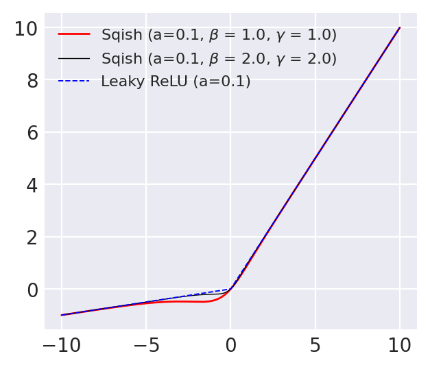
Figure 1: Approximation of Leaky ReLU ($a=0.1$) using Sqish ($a=0.1$) for different values of $\beta$ and $\gamma$. As $\gamma\rightarrow\infty$, Sqish smoothly approximate Leaky ReLU.

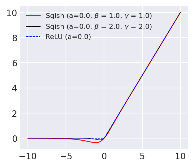
Figure 2: Approximation of ReLU using Sqish for different values of $\beta$ and $\gamma$. As $\gamma\rightarrow\infty$, Sqish smoothly approximates ReLU.

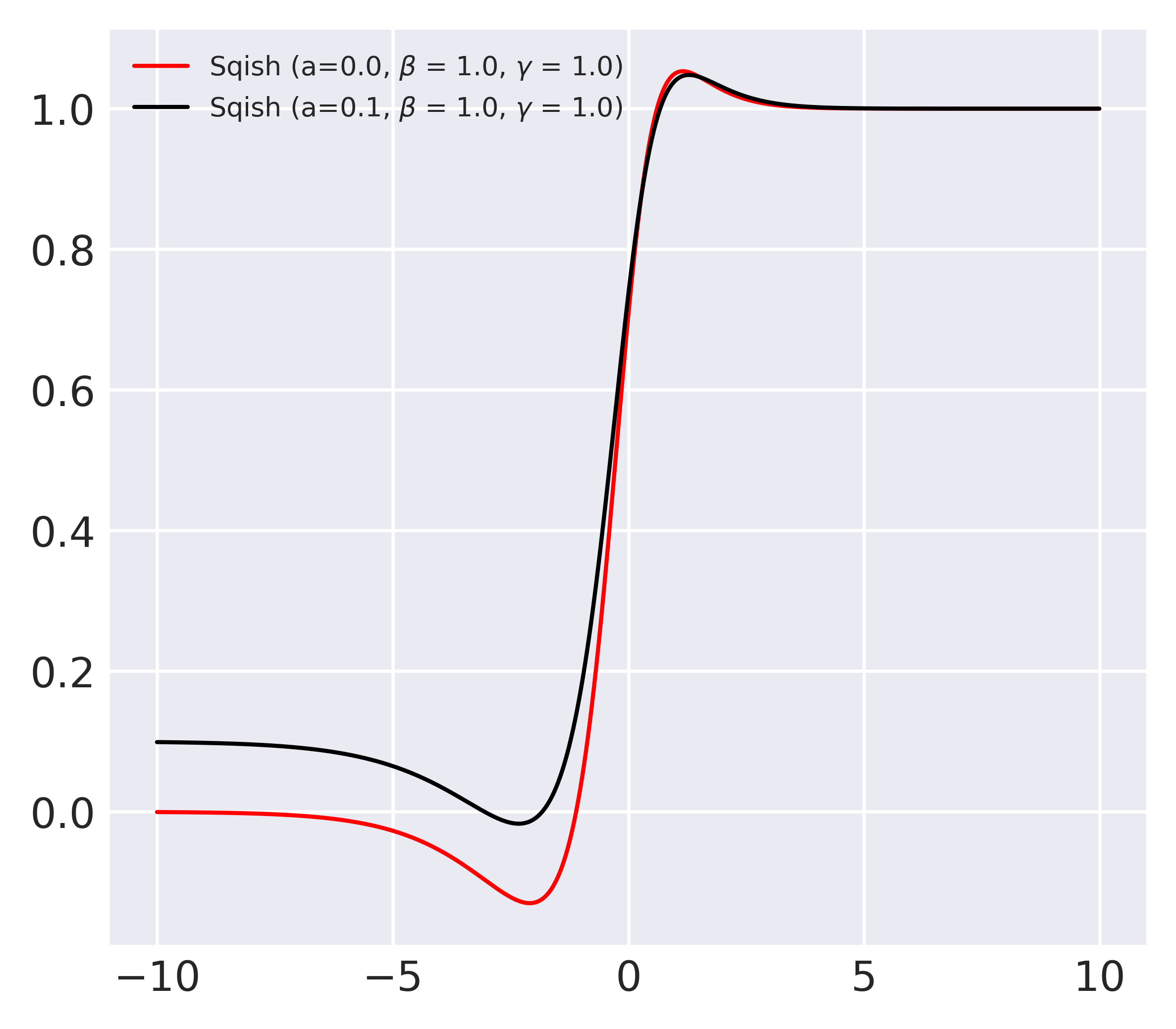
Figure 3: First order derivatives of Sqish with respect to ’x’ for different values of $a$, $\beta$ and $\gamma$.

An idea behind equation (2) is given in the supplementary document. It is a known fact that the maximum function is not differentiable in the real line. Now, note that the second term in equation (2) is not differentiable. We can get a smooth function from equation (2) by using an approximation of the maximum function by a smooth function. We have proposed a new approximation of the $max(0,x)$ function, which is defined as follows:

$$F(x;\gamma)=\dfrac{x}{\sqrt{1+e^{-2\gamma x}}},\ \ \ \gamma>0$$ (3)

Note that, if we consider $\gamma\rightarrow\infty$, We have $f(x;\gamma)$ $\rightarrow$ $max(0,x)$. The function in equation (3) is a smooth function in the real line. Replacing the second term in equation (2) by the approximation proposed in equation (3), we have a pointwise approximation formula by a smooth function for the maximum function as follows:

$$f(x_{1},x_{2};\gamma) =x_{1}+\dfrac{(x_{2}-x_{1})}{\sqrt{1+e^{-2\gamma(x_{2}-x_{1})}}},\ \ \ \gamma>0$$ (4)

Note that if we consider $\gamma\rightarrow\infty$, we have $f(x_{1},x_{2};\gamma)\rightarrow max(x_{1},x_{2})$. We can get known activation functions for specific values of $x_{1}$ and $x_{2}$. Equation (4) can approximate the Maxout family. In particular, consider $x_{1}=ax$ and $x_{2}=bx$, we have,

$$f(ax,bx;\gamma) =x_{1}+\dfrac{(bx-ax)}{\sqrt{1+e^{-2\gamma(bx-ax)}}},\ \ \ \gamma>0$$ (5)

This is a very simple case from the Maxout family, but we can derive a more complex formula by considering different values of $x_{1}$ and $x_{2}$. Now, considering $x_{1}=0$ and $x_{2}=x$, we have an approximation of the ReLU activation function by a smooth function.

$$f(0,x;\gamma) =\dfrac{x}{\sqrt{1+e^{-2\gamma x}}},\ \ \ \gamma>0$$ (6)

Similarly, we can derive an approximation of the Leaky ReLU activation (or parametric ReLU, depending on if ‘a’ is a hyperparameter or a trainable parameter) function by considering $x_{1}=ax$ and $x_{2}=x$.

$$f(ax,x;\gamma)=ax+\dfrac{(1-a)x}{\sqrt{1+e^{-2\gamma(1-a)x}}},\ \ \ \gamma>0$$ (7)

We have introduced another parameter $\beta$ in equation (7) as follows:

$$f(ax,x;\beta,\gamma)=ax+\dfrac{(1-a)x}{\sqrt{1+\beta e^{-2\gamma(1-a)x}}},\ \beta>0,\gamma>0$$ (8)

$\beta$ will control the function smoothness in both negative and positive axes in the real line. For the rest of the paper, we will use equation (8) as our proposed activation function, which we call Sqish. Figure 3,  3, and  3 represent the plots for Sqish and its derivative for different values of $a,\beta,$ and $\gamma$.

The derivative of the proposed function in equation (8) with respect to the variable $x$ is

$$\frac{\partial f(x;a,\beta,\gamma)}{\partial x}=a+\dfrac{1-a}{\sqrt{{\beta}\mathrm{e}^{-2\left(1-a\right){\gamma}x}+1}}$$ (9)

$$+\dfrac{\left(1-a\right)^{2}{\beta}{\gamma}x\mathrm{e}^{-2\left(1-a\right){\gamma}x}}{\left({\beta}\mathrm{e}^{-2\left(1-a\right){\gamma}x}+1\right)^{\frac{3}{2}}}$$

4.2 Learning Activation parameter

The proposed activation function in equation (8) has parameters that can be used as hyperparameters (as a fixed activation function) or trainable parameters (as a trainable activation function). Trainable parameters in a trainable activation function are updated using the backpropagation algorithm LeCun et al. (1989). Gradients with respect to the parameters $a,\beta,\text{and}\ \gamma$ can be computed as follows:

$$\frac{\partial f(x;a,\beta,\gamma)}{\partial a}=x-\dfrac{x}{\sqrt{{\beta}\mathrm{e}^{-2x{\gamma}\cdot\left(1-a\right)}+1}}$$ (10)

$$-\dfrac{{\beta}x^{2}{\gamma}\cdot\left(1-a\right)\mathrm{e}^{-2x{\gamma}\cdot\left(1-a\right)}}{\left({\beta}\mathrm{e}^{-2x{\gamma}\cdot\left(1-a\right)}+1\right)^{\frac{3}{2}}}$$

$$\frac{\partial f(x;a,\beta,\gamma)}{\partial\beta}=\dfrac{\left(a-1\right)x\mathrm{e}^{-2\left(1-a\right)x{\gamma}}}{2\left(\mathrm{e}^{-2\left(1-a\right)x{\gamma}}{\beta}+1\right)^{\frac{3}{2}}}$$ (11)

$$\frac{\partial f(x;a,\beta,\gamma)}{\partial\gamma}=\dfrac{\left(a-1\right)^{2}{\beta}x^{2}\mathrm{e}^{-2\left(1-a\right)x{\gamma}}}{\left({\beta}\mathrm{e}^{-2\left(1-a\right)x{\gamma}}+1\right)^{\frac{3}{2}}}$$ (12)

Note that $a$, $\beta$, and $\gamma$ can be used as hyperparameters or trainable parameters.

Now, note that the class of neural networks with Sqish activation function is dense in $C(K)$, where $K$ is a compact subset of $\mathbb{R}^{n}$ and $C(K)$ is the space of all continuous functions over $K$.
The proof follows from the following theorem.

Theorem 1.1 from Kidger and Lyons, 2020 Kidger and Lyons (2020):- Let $\rho:\mathbb{R}\rightarrow\mathbb{R}$ be any continuous function. Let $N_{n}^{\rho}$ represent the class of neural networks with activation function $\rho$, with $n$ neurons in the input layer, one neuron in the output layer, and one hidden layer with an arbitrary number of neurons. Let $K\subseteq\mathbb{R}^{n}$ be compact. Then $N_{n}^{\rho}$ is dense in $C(K)$ if and only if $\rho$ is non-polynomial.

5 Experiments:

The following subsections present a detailed experimental evaluation of different deep-learning problems with standard datasets. To compare performance with Sqish, we consider eight widely used activation functions- ReLU, Leaky ReLU, PReLU, ELU, Swish, GELU, Mish, and PAU as baseline activation functions. All the experiments are conducted on NVIDIA RTX 3090 and NVIDIA Tesla A100 GPUs. Swish, PReLU, PAU, and Sqish (the proposed function) are considered trainable activation functions, and the trainable parameters are updated via the backpropagation algorithm LeCun et al. (1989).

5.1 Image Classification

We report detailed experimental results on the image classification problem with MNIST LeCun et al. (2010), Fashion MNISTXiao et al. (2017), SVHN Netzer et al. (2011), CIFAR10 Krizhevsky (2009), CIFAR100 Krizhevsky (2009), and Tiny Imagenet Le and Yang (2015) datasets. Details are given in the following subsections.

5.1.1 MNIST, Fashion MNIST, and SVHN

In this section, we have reported results with MNIST LeCun et al. (2010), Fashion MNISTXiao et al. (2017), and SVHN Netzer et al. (2011) datasets. There are a total of 60k training images and 10k test images in the $28\times 28$ greyscale format in the MNIST and Fashion MNIST databases in 10 distinct classes. SVHN database includes 73257 training images and 26032 test images. All the images are in $32\times 32$ RGB format with ten distinct classes. Basic data augmentation methods like zoom and rotation are applied to the SVHN dataset. We take into account a batch size of 128, 0.01 initial learning rate, and cosine annealing learning rate scheduler Loshchilov and Hutter (2017) to decay the learning rate. We train all networks up to 100 epochs using stochastic gradient descent Robbins and Monro (1951); Kiefer and Wolfowitz (1952) optimizer with 0.9 momentum & $5e^{-4}$ weight decay. For the mean of 5 distinct runs, we report our results using the AlexNet architecture Krizhevsky et al. (2012) in Table 1.

Activation Function	MNIST	Fashion MNIST	SVHN
ReLU	$99.44\pm 0.08$	$92.68\pm 0.21$	$95.07\pm 0.14$
Leaky ReLU	$99.44\pm 0.09$	$92.72\pm 0.17$	$95.12\pm 0.16$
PReLU	99.47 $\pm$ 0.08	92.71 $\pm$ 0.18	95.04 $\pm$ 0.14
ELU	$99.49\pm 0.06$	$92.88\pm 0.13$	$95.11\pm 0.15$
GELU	99.56$\pm$ 0.06	93.01 $\pm$ 0.14	95.12 $\pm$ 0.12
Swish	$99.55\pm 0.05$	$92.88\pm 0.16$	$95.28\pm 0.15$
PAU	$99.53\pm 0.11$	93.10 $\pm$ 0.16	95.26 $\pm$ 0.17
Mish	$99.62\pm 0.06$	93.16 $\pm$ 0.14	95.37 $\pm$ 0.11
Sqish	99.67 $\pm$ 0.06	93.35 $\pm$ 0.12	95.60 $\pm$ 0.11

Table 1: Comparison between Sqish and other baseline activations on MNIST, Fashion MNIST, and SVHN datasets for image classification problem on AlexNet architecture. We report Top-1 test accuracy (in %) for the mean of 5 different runs. mean$\pm$std is reported in the Table.

5.1.2 CIFAR

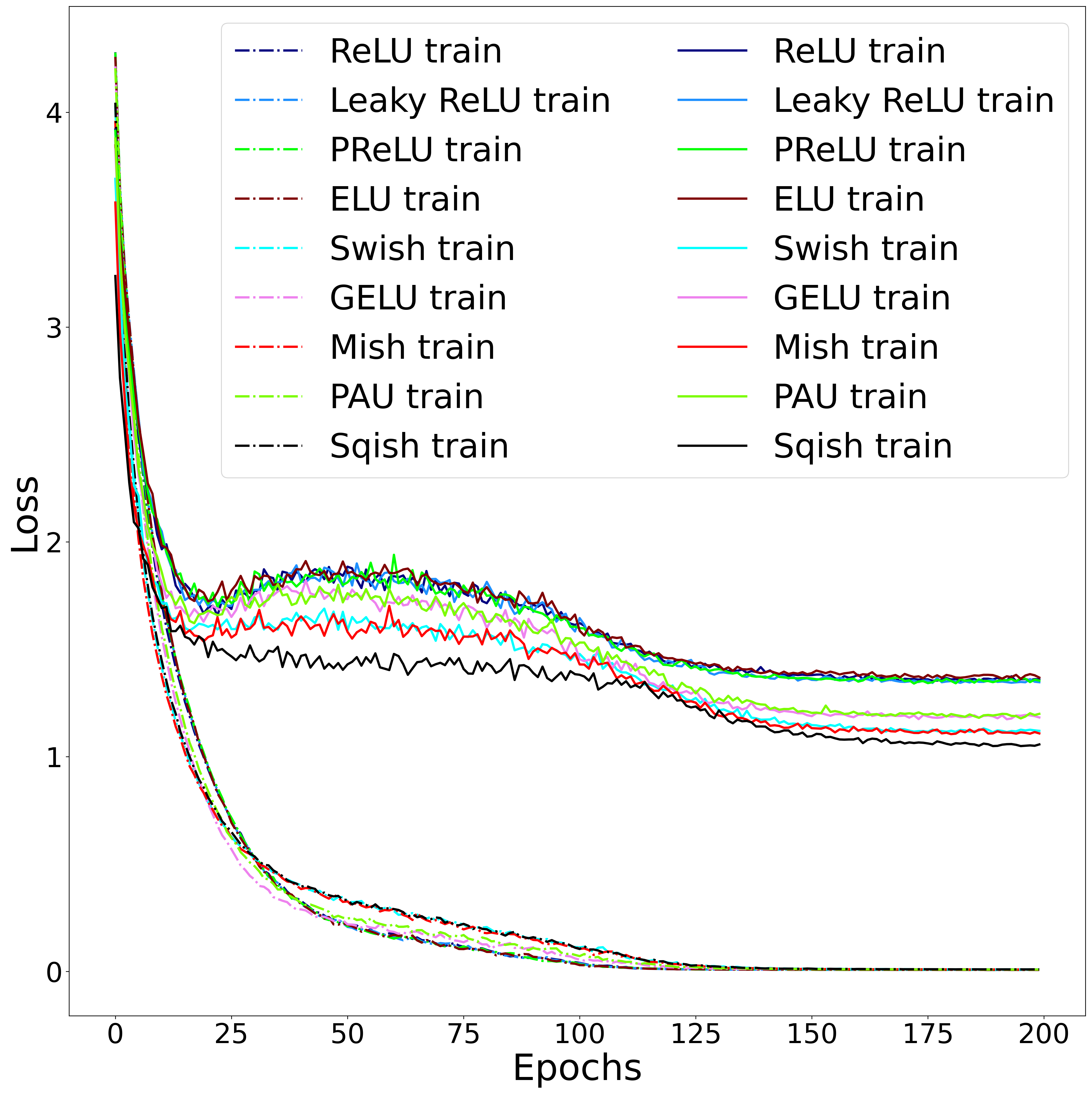
Figure 5: Top-1 train and test loss curves for Sqish and other baseline activation functions on CIFAR100 dataset with ShuffleNet V2.

In this section, we present results from the standard image classification datasets CIFAR10 Krizhevsky (2009) and CIFAR100 Krizhevsky (2009). Both datasets contain 50k training and 10k testing photos. CIFAR10 has ten classes, while CIFAR100 offers 100 classes. In these two datasets, we consider a batch size of 128, 0.01 initial learning rate, and decay the learning rate with cosine annealing learning rate scheduler Loshchilov and Hutter (2017). We use stochastic gradient descent Robbins and Monro (1951); Kiefer and Wolfowitz (1952) optimizer with 0.9 momentum & $5e^{-4}$ weight decay and trained all networks up to 200 epochs. We use data augmentation methods, including horizontal flipping and rotation. Top-1 accuracy is presented in Table 3 and Table 2 for the CIFAR10 and CIFAR100 datasets, respectively, for a mean of 10 different runs. We report results with AlexNet (An) Krizhevsky et al. (2012), LeNet (LN) Lecun et al. (1998), VGG-16 Simonyan and Zisserman (2015), WideResNet 28-10 (WRN 28-10) Zagoruyko and Komodakis (2016), ResNet (RN) He et al. (2015b), PreActResNet (PARN) He et al. (2016), DenseNet-121 (DN 121) Huang et al. (2016), Inception V3 (IN V3) Szegedy et al. (2015), MobileNet V2 (MN V2) Sandler et al. (2019), ResNext (RNxt) Xie et al. (2017), Xception (XT) Chollet (2017), and EfficientNet B0 (EN B0) Tan and Le (2020). The learning curves on the CIFAR100 dataset with the ShuffleNet V2 (2.0x) model for the baseline and Sqish are given in Figures 5 and  5.

Activation Function

AN

LN

VGG 16

WRN 28-10

RN 50

PARN 34

DN 121

IN V3

MN V2

SF-V2 2.0x

RNxt

XT

EN B0

RN 18

ReLU

54.98 $\pm$0.26

45.35 $\pm$0.27

71.62 $\pm$0.25

76.39 $\pm$0.23

74.28 $\pm$0.22

73.23 $\pm$0.20

75.60 $\pm$0.25

74.33 $\pm$0.24

74.00 $\pm$0.22

67.49 $\pm$0.26

74.40 $\pm$0.22

71.18 $\pm$0.24

76.63 $\pm$0.23

73.12 $\pm$0.22

Leaky ReLU

55.20 $\pm$0.26

45.60 $\pm$0.25

71.76 $\pm$0.26

76.56 $\pm$0.24

74.20 $\pm$0.25

73.35 $\pm$0.24

75.79 $\pm$0.25

74.32 $\pm$0.25

74.20 $\pm$0.22

67.61 $\pm$0.25

74.50 $\pm$0.25

71.10 $\pm$0.25

76.89 $\pm$0.26

73.05 $\pm$0.24

PReLU

55.62 $\pm$0.26

45.50 $\pm$0.26

71.85 $\pm$0.31

76.77 $\pm$0.25

74.40 $\pm$0.27

73.20 $\pm$0.28

76.10 $\pm$0.28

74.40 $\pm$0.28

74.42 $\pm$0.33

68.45 $\pm$0.27

74.55 $\pm$0.25

71.25 $\pm$0.26

76.70 $\pm$0.28

73.19 $\pm$0.24

ELU

55.81 $\pm$0.27

46.10 $\pm$0.28

71.83 $\pm$0.26

76.50 $\pm$0.29

74.40 $\pm$0.23

73.69 $\pm$0.26

75.99 $\pm$0.28

74.62 $\pm$0.27

74.43 $\pm$0.24

67.89 $\pm$0.28

74.70 $\pm$0.23

71.59 $\pm$0.26

76.73 $\pm$0.28

73.33 $\pm$0.26

Swish

57.72 $\pm$0.24

47.42 $\pm$0.25

72.15 $\pm$0.24

77.11 $\pm$0.25

75.19 $\pm$0.23

73.90 $\pm$0.25

76.40 $\pm$0.28

75.45 $\pm$0.28

75.15 $\pm$0.27

71.45 $\pm$0.28

75.20 $\pm$0.25

72.30 $\pm$0.22

77.22 $\pm$0.22

73.68 $\pm$0.24

Mish

58.37 $\pm$0.22

47.52 $\pm$0.26

72.50 $\pm$0.24

77.50 $\pm$0.27

76.43 $\pm$0.24

75.11 $\pm$0.24

77.01 $\pm$0.26

76.23 $\pm$0.23

75.21 $\pm$0.22

71.93 $\pm$0.24

76.29 $\pm$0.25

73.50 $\pm$0.23

78.23 $\pm$0.23

74.60 $\pm$0.21

GELU

57.38 $\pm$0.25

47.26 $\pm$0.29

71.90 $\pm$0.24

77.47 $\pm$0.27

75.60 $\pm$0.23

74.18 $\pm$0.25

76.88 $\pm$0.24

75.63 $\pm$0.25

75.30 $\pm$0.20

70.56 $\pm$0.26

75.27 $\pm$0.23

72.15 $\pm$0.23

77.21 $\pm$0.21

73.99 $\pm$0.24

PAU

57.69 $\pm$0.24

47.40 $\pm$0.27

71.56 $\pm$0.26

77.32 $\pm$0.27

75.92 $\pm$0.22

74.36 $\pm$0.24

76.69 $\pm$0.26

75.86 $\pm$0.25

75.10 $\pm$0.20

71.10 $\pm$0.24

75.79 $\pm$0.25

72.70 $\pm$0.26

77.50 $\pm$0.25

74.10 $\pm$0.20

Sqish

61.09 $\pm$0.24

47.00 $\pm$0.24

73.10 $\pm$0.20

78.66 $\pm$0.22

77.29 $\pm$0.18

76.44 $\pm$0.20

78.12 $\pm$0.21

77.02 $\pm$0.21

76.36 $\pm$0.20

73.36 $\pm$0.18

77.10 $\pm$0.22

74.30 $\pm$0.21

78.50 $\pm$0.22

75.02 $\pm$0.21

Table 2: Comparison between different baseline activations and Sqish on CIFAR100 dataset. Top-1 accuracy(in $\%$) for a mean of 10 different runs has been reported. mean$\pm$std is reported in the Table.

Activation Function

AN

LN

VGG 16

WRN 28-10

RN 50

PARN 34

DN 121

IN V3

MN V2

SF-V2 2.0x

RNxt

XT

EN B0

RN 18

ReLU

84.15 $\pm$0.18

75.87 $\pm$0.18

93.50 $\pm$0.20

95.25 $\pm$0.18

94.42 $\pm$0.19

94.10 $\pm$0.18

94.68 $\pm$0.17

94.22 $\pm$0.22

94.22 $\pm$0.19

91.65 $\pm$0.24

93.35 $\pm$0.19

90.56 $\pm$0.24

95.12 $\pm$0.17

94.17 $\pm$0.22

Leaky ReLU

84.20 $\pm$0.20

75.99 $\pm$0.18

93.60 $\pm$0.18

95.10 $\pm$0.21

94.40 $\pm$0.18

94.25 $\pm$0.20

94.80 $\pm$0.20

94.11 $\pm$0.19

94.25 $\pm$0.16

91.70 $\pm$0.20

93.30 $\pm$0.19

90.80 $\pm$0.24

95.30 $\pm$0.17

94.10 $\pm$0.24

PReLU

84.36 $\pm$0.21

75.89 $\pm$0.22

93.18 $\pm$0.20

94.94 $\pm$0.22

94.21 $\pm$0.24

94.28 $\pm$0.26

94.45 $\pm$0.22

94.41 $\pm$0.24

94.38 $\pm$0.20

91.75 $\pm$0.22

93.39 $\pm$0.20

91.15 $\pm$0.23

95.32 $\pm$0.18

94.20 $\pm$0.25

ELU

84.75 $\pm$0.21

75.82 $\pm$0.20

93.68 $\pm$0.120

95.21 $\pm$0.18

94.24 $\pm$0.25

94.21 $\pm$0.25

94.51 $\pm$0.19

94.50 $\pm$0.20

94.21 $\pm$0.19

91.88 $\pm$0.22

93.50 $\pm$0.16

91.39 $\pm$0.20

95.43 $\pm$0.15

94.20 $\pm$0.22

Swish

85.34 $\pm$0.18

77.93 $\pm$0.18

93.69 $\pm$0.19

95.34 $\pm$0.18

94.59 $\pm$0.22

94.57 $\pm$0.24

94.69 $\pm$0.20

94.43 $\pm$0.18

94.48 $\pm$0.17

92.24 $\pm$0.22

93.69 $\pm$0.18

91.78 $\pm$0.20

95.63 $\pm$0.16

94.035 $\pm$0.22

Mish

85.85 $\pm$0.18

77.85 $\pm$0.17

93.90 $\pm$0.16

95.25 $\pm$0.16

94.70 $\pm$0.20

94.60 $\pm$0.20

95.14 $\pm$0.17

94.70 $\pm$0.17

94.70 $\pm$0.20

92.50 $\pm$0.18

93.90 $\pm$0.17

92.11 $\pm$0.22

95.61 $\pm$0.15

94.60 $\pm$0.23

GELU

85.12 $\pm$0.20

77.39 $\pm$0.18

93.70 $\pm$0.22

95.33 $\pm$0.24

94.88 $\pm$0.20

94.67 $\pm$0.18

94.47 $\pm$0.19

94.35 $\pm$0.18

94.30 $\pm$0.17

92.39 $\pm$0.18

93.55 $\pm$0.19

91.92 $\pm$0.21

95.42 $\pm$0.16

94.39 $\pm$0.21

PAU

85.25 $\pm$0.21

77.69 $\pm$0.21

93.50 $\pm$0.21

95.19 $\pm$0.18

94.60 $\pm$0.20

94.39 $\pm$0.22

94.77 $\pm$0.18

94.50 $\pm$0.17

94.41 $\pm$0.16

92.22 $\pm$0.18

93.59 $\pm$0.17

92.09 $\pm$0.21

95.41 $\pm$0.17

94.31 $\pm$0.21

Sqish

86.79 $\pm$0.18

77.36 $\pm$0.20

94.51 $\pm$0.11

95.71 $\pm$0.12

95.32 $\pm$0.15

95.07 $\pm$0.18

95.68 $\pm$0.17

95.32 $\pm$0.14

95.40 $\pm$0.12

93.79 $\pm$0.17

94.36 $\pm$0.19

92.79 $\pm$0.21

96.04 $\pm$0.14

94.96 $\pm$0.18

Table 3: Comparison between different baseline activations and Sqish on CIFAR10 dataset. Top-1 accuracy(in $\%$) for a mean of 10 different runs has been reported. mean$\pm$std is reported in the Table.

5.1.3 Tiny ImageNet

In this section, we delve into the intricacies of image classification using the challenging Tiny Imagenet dataset Le and Yang (2015). Tiny Imagenet presents a rich tapestry of $64\times 64$ RGB visuals, encompassing 1,00,000 training snapshots, 10,000 for validation, and another 10,000 designated for testing, all distributed across 200 diverse classes. To enhance the robustness of our model, we incorporated augmentation strategies, including rotation and horizontal flipping. Our experimental setup involves a batch size set to 64 and an initial learning rate of 0.1. Notably, we apply a meticulous reduction in this rate by a factor of 10 after every successive 50 epochs. The optimization landscape is carved using stochastic gradient descent (SGD) Robbins and Monro (1951); Kiefer and Wolfowitz (1952), complemented by a 0.9 momentum and a weight decay of $5e^{-4}$. Each network was rigorously trained over 200 epochs. For a comprehensive view, Table 4 presents the top-1 accuracy, representing an average over five distinct runs.

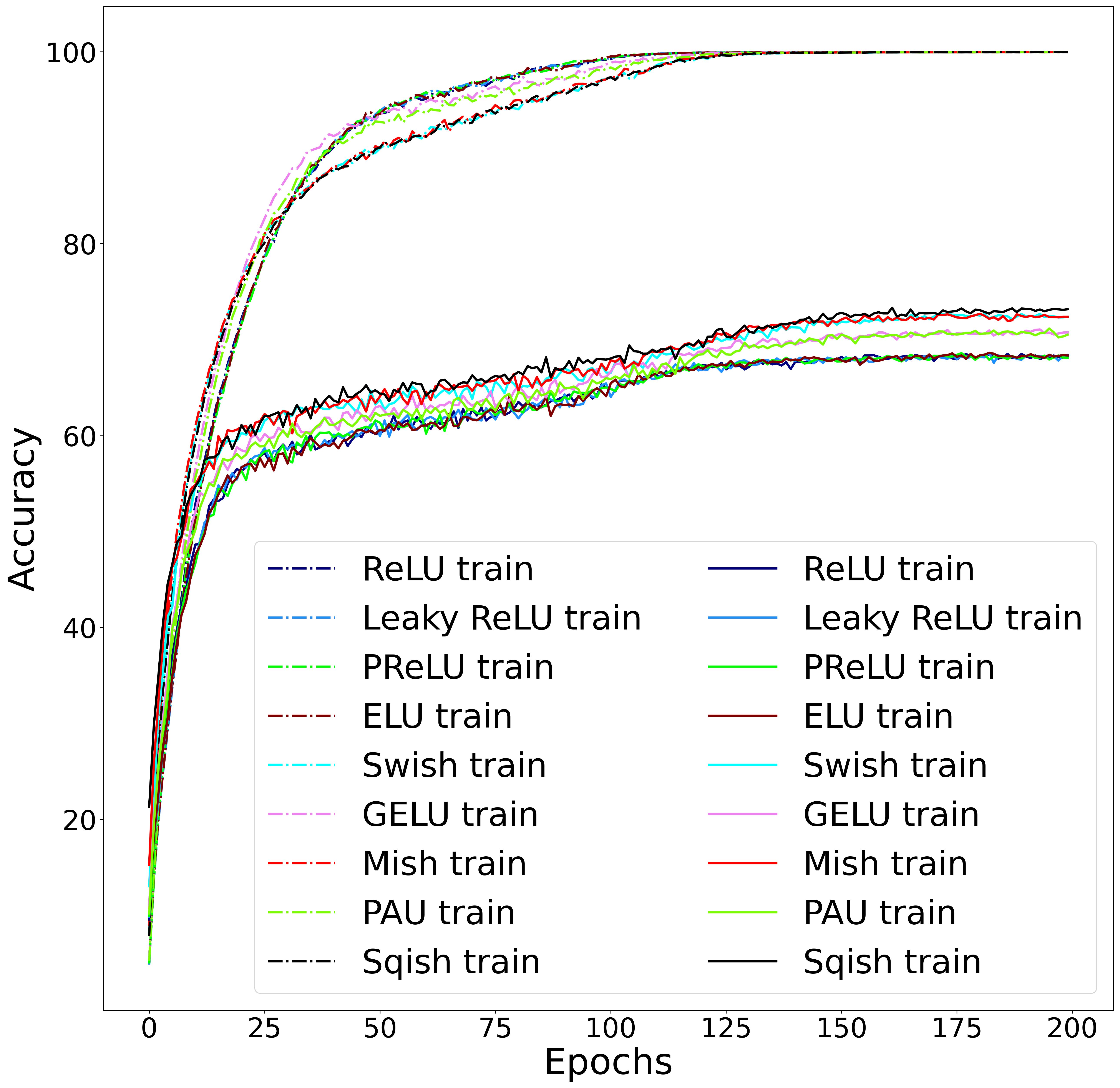
Figure 4: Top-1 train and test accuracy curves for Sqish and other baseline activation functions on CIFAR100 dataset with ShuffleNet V2.

Activation Function	ResNet-18	ResNet-50	WideResNet 28-10
ReLU	59.21 $\pm$ 0.40	61.11 $\pm$ 0.42	63.60 $\pm$ 0.37
Leaky ReLU	59.31 $\pm$ 0.41	61.41 $\pm$ 0.41	63.49 $\pm$ 0.39
PReLU	59.69 $\pm$ 0.39	61.42 $\pm$ 0.41	63.71 $\pm$ 0.42
ELU	59.28 $\pm$ 0.41	61.34 $\pm$ 0.40	63.79 $\pm$ 0.41
Swish	60.21 $\pm$ 0.41	61.69 $\pm$ 0.40	64.50 $\pm$ 0.38
Mish	60.32 $\pm$ 0.36	62.20 $\pm$ 0.40	64.81 $\pm$ 0.36
GELU	60.20 $\pm$ 0.36	61.89 $\pm$ 0.40	64.32 $\pm$ 0.35
PAU	60.51 $\pm$ 0.37	61.81 $\pm$ 0.40	64.51 $\pm$ 0.36
Sqish	61.20 $\pm$ 0.36	63.05 $\pm$ 0.38	65.92 $\pm$ 0.33

Table 4: Comparison between Squish and other baseline activations on Tiny ImageNet dataset for image classification problem. We report Top-1 test accuracy (in %) for the mean of 5 different runs. mean$\pm$std is reported in the Table.

5.2 Object Detection

In this section, we provide experimental results for the object detection task on the Pascal VOC dataset Everingham et al. (2010) using the Single Shot MultiBox Detector (SSD) 300 model Liu et al. (2016) and consider VGG16 (with batch-normalization) Simonyan and Zisserman (2015) as the backbone network. VOC2007 and VOC2012 are used as train data, and VOC2007 is used as the test dataset. There are 20 distinct objects in the dataset. We assume a batch size of 8 and an initial learning rate of 0.001. We employ the SGD Robbins and Monro (1951); Kiefer and Wolfowitz (1952) optimizer with 0.9 momentum and $5e^{-4}$ weight decay, as well as trained networks with up to 120000 iterations. We do not take into account any pre-trained weight. Table 5 shows the mean average accuracy (mAP) for the mean of five separate runs.

Activation Function	mAP
ReLU	77.3 $\pm$ 0.13
Leaky ReLU	77.2 $\pm$ 0.15
PReLU	77.3 $\pm$ 0.14
ELU	77.3 $\pm$ 0.15
Swish	77.5 $\pm$ 0.12
Mish	77.6 $\pm$ 0.12
GELU	77.5 $\pm$ 0.14
PAU	77.5 $\pm$ 0.13
Sqish	78.1 $\pm$ 0.09

Table 5: Comparison between Sqish and other baseline activations on Pascal VOC dataset for object detection problem. We report mAP for the mean of 5 different runs. mean$\pm$std is reported in the Table.

5.3 3D Medical Imaging

In the following subsections, we report detailed experimental results on 3D medical image classification and 3D medical image segmentation problems.

5.3.1 3D Medical Image Classification

This section presents experimental results for the 3D image classification problem on MosMed dataset Morozov et al. (2020). The dataset contains CT scans with COVID-19-related findings (CT1-CT4) and without any findings (CT0). The dataset has 1110 studies. We consider 70% of the data as training data and 30% of the data used for testing. We consider a batch size of 8, 0.0001 initial learning rate, and decay the learning rate with cosine annealing learning rate scheduler Loshchilov and Hutter (2017). We use Adam optimizer Kingma and Ba (2015), $5e^{-4}$ weight decay, and trained up to 200 epochs with 3D ResNet-18 model. Experimental results are reported in Table 6.

Activation Function	Accuracy
ReLU	79.50
Leaky ReLU	79.67
PReLU	79.76
ELU	79.89
Swish	79.99
Mish	80.17
GELU	79.96
PAU	80.27
Sqish	80.58

Table 6: Comparison between Sqish and other baseline activations on MosMedData dataset for 3D image classification with ResNet-18 model. We report Top-1 accuracy for the mean of 5 different runs.

5.3.2 3D Medical Image Segmentation

This section presents the experimental outcomes for 3D brain tumor segmentation using 3D-UNet Özgün Çiçek et al. (2016) on the BraTS 2020 dataset Menze et al. (2014); Bakas et al. (2017, 2018). This data set contains 369 samples for training and 125 samples for validation. In this experiment, we consider a batch size of 2, and the learning rate is 0.001, Adam optimizer Kingma and Ba (2015) with $5e^{-4}$ weight decay and cosine annealing learning rate scheduler for training the network. Moreover, we trained this 3D model for 150 epochs. We presented the network performance analysis for Sqish and the baseline activation functions with this network in Table 7 in terms of Accuracy and Dice Score to measure the performance.

Activation Function	Accuracy	Dice Score
ReLU	95.04	97.37
Leaky ReLU	94.98	97.34
PReLU	94.95	97.40
ELU	95.10	97.42
Swish	95.17	97.50
Mish	95.12	97.48
GELU	95.21	97.30
PAU	95.27	97.54
Sqish	95.45	97.68

Table 7: Comparison between Sqish and other baseline activations on BraTS 2020 Dataset for 3D image segmentation with 3D-Unet Model.

5.4 Adversarial Attack

In our investigation of adversarial attack challenges, we utilized the CIFAR10 and CIFAR100 datasets, coupling them with the FGSM attack methodology Goodfellow et al. (2015). These datasets were processed with a batch size of 128 and an initial learning rate of 0.01. As we navigated through our experiment, the learning rate underwent a nuanced decay, facilitated by the cosine annealing learning rate scheduler Loshchilov and Hutter (2017). The optimization frontier was led by the stochastic gradient descent Robbins and Monro (1951); Kiefer and Wolfowitz (1952), fortified with a momentum of 0.9 and a weight decay setting of $5e^{-4}$. Throughout this scientific endeavor, every network was diligently trained over a span of 200 epochs.

For the discerning reader, we’ve tabulated the Top-1 accuracy in Table 8 (for CIFAR10) and Table 9 (for CIFAR100). These results represent an average derived from 10 distinct runs. Our research spotlight was on the robust frameworks of ShuffleNet V2 (2.0x) Ma et al. (2018) and MobileNet V2 Sandler et al. (2019).

Activation Function	ShuffleNet V2 (2.0x)	MobileNet V2
ReLU	59.26 $\pm$ 0.11	68.89 $\pm$ 0.14
Leaky ReLU	59.87 $\pm$ 0.12	68.81 $\pm$ 0.15
PReLU	60.15 $\pm$ 0.10	69.06 $\pm$ 0.13
ELU	60.36 $\pm$ 0.11	69.22 $\pm$ 0.14
Swish	65.66 $\pm$ 0.10	69.81 $\pm$ 0.12
Mish	65.42 $\pm$ 0.12	70.10 $\pm$ 0.12
GELU	64.84 $\pm$ 0.11	69.55 $\pm$ 0.14
PAU	66.10 $\pm$ 0.10	69.99 $\pm$ 0.14
Sqish	68.47 $\pm$ 0.09	70.68 $\pm$ 0.12

Table 8: Comparison between Sqish and other baseline activations on CIFAR100 dataset for FGSM Adversarial attack ($\epsilon=0.04)$. We report Top-1 accuracy for the mean of 5 different runs. mean$\pm$std is reported in the Table.

Activation Function	ShuffleNet V2 (2.0x)	MobileNet V2
ReLU	87.41 $\pm$ 0.14	90.52 $\pm$ 0.15
Leaky ReLU	87.59 $\pm$ 0.13	90.67 $\pm$ 0.12
PReLU	87.85 $\pm$ 0.14	90.60 $\pm$ 0.14
ELU	87.92 $\pm$ 0.16	90.80 $\pm$ 0.14
Swish	89.69 $\pm$ 0.12	91.35 $\pm$ 0.12
Mish	89.35 $\pm$ 0.11	91.68 $\pm$ 0.13
GELU	89.02 $\pm$ 0.12	91.33 $\pm$ 0.14
PAU	89.94 $\pm$ 0.12	91.74 $\pm$ 0.13
Sqish	91.15 $\pm$ 0.12	92.20 $\pm$ 0.12

Table 9: Comparison between Sqish and other baseline activations on CIFAR10 dataset for FGSM Adversarial attack ($\epsilon=0.04)$. We report Top-1 accuracy for the mean of 5 different runs. mean$\pm$std is reported in the Table.

Baselines	ReLU	Leaky ReLU	ELU	PReLU	Swish	Mish	GELU	PAU
Sqish $>$ Baseline	43	43	43	43	43	43	43	43
Sqish $=$ Baseline	0	0	0	0	0	0	0	0
Sqish $<$ Baseline	0	0	0	0	2	2	2	2

Table 10: Baseline table for Sqish. These numbers represent the total number of models in which Sqish underperforms, equals, or outperforms compared with the baseline activation functions

5.5 Data Augmentation

In this section, we report results with the MixUp Zhang et al. (2018) augmentation method. Mixup augmentation is a data augmentation method that uses the training data to produce a weighted combination of random image pairings. Mixup augmentation can assist in preventing overfitting, increasing generalization, and strengthening the model against adversarial attacks. We report results with Mixup augmentation on the CIFAR100 dataset with the ShuffleNet V2 Ma et al. (2018) and ResNet-18 He et al. (2015b) model on Table 11. To train the network, we consider a batch size of 128, 0.01 initial learning rate, and decay the learning rate with cosine annealing learning rate scheduler Loshchilov and Hutter (2017), stochastic gradient descent Robbins and Monro (1951); Kiefer and Wolfowitz (1952) optimizer with 0.9 momentum & $5e^{-4}$ weight decay, and trained up to 200 epochs.

Activation Function	ShuffleNet V2 (2.0x)	ResNet 18
ReLU	69.18 $\pm$ 0.20	73.79 $\pm$ 0.21
Leaky ReLU	69.15 $\pm$ 0.20	73.90 $\pm$ 0.23
PReLU	69.18 $\pm$ 0.22	74.10 $\pm$ 0.22
ELU	69.30 $\pm$ 0.20	74.21 $\pm$ 0.21
Swish	72.69 $\pm$ 0.20	74.42 $\pm$ 0.21
Mish	72.98 $\pm$ 0.20	74.60 $\pm$ 0.21
GELU	72.90 $\pm$ 0.21	74.45 $\pm$ 0.22
PAU	73.39 $\pm$ 0.20	74.80 $\pm$ 0.21
Sqish	74.40 $\pm$ 0.18	75.85 $\pm$ 0.18

Table 11: Top-1 Test Accuracy Reported with Mixup Augmentation Method on CIFAR100 Dataset for the Mean of 5 Different Runs. We Report mean$\pm$std in the Table.

6 Baseline Table

We present a detailed experimental summary in Table 10. This Table shows the total number of experiments conducted and the total number of cases where the proposed function outperforms, equals, or underperforms compared with the baseline activation functions. From the baseline table, it is clear that Sqish outperforms baseline activations in most cases.

7 Computational Time Comparison

We present the computational Time Comparison for Sqish and the baseline activation functions in this section. The tests are carried out on an NVIDIA Tesla A100 GPU. The results are reported in Table 12 for Sqish and other baseline activation functions for a 224 $\times$ 224 RGB image in the ResNet-18 model. From the experiment section and Table 12, it is clear that there is a trade-off between computational time and model performance when compared to ReLU or its variants, as Sqish is highly non-linear. Also, note that Sqish improves model performance significantly while training time is comparable with smooth activations like Swish, Mish, GELU, & PAU.

Activation Function	Forward Pass	Backward Pass
ReLU	3.83 $\pm$ 0.64 $\mu$s	5.17 $\pm$ 0.58 $\mu$s
Leaky ReLU	4.32 $\pm$ 0.11 $\mu$s	5.20 $\pm$ 0.13 $\mu$s
PReLU	5.11 $\pm$ 0.32$\mu$s	6.15 $\pm$ 0.33 $\mu$s
ELU	4.41 $\pm$ 0.58 $\mu$s	5.40 $\pm$ 0.38 $\mu$s
Mish	6.71 $\pm$ 1.69 $\mu$s	6.58 $\pm$ 0.44 $\mu$s
GELU	5.50 $\pm$ 0.21 $\mu$s	7.52 $\pm$ 0.31 $\mu$s
Swish	5.47 $\pm$ 0.14 $\mu$s	6.78 $\pm$ 0.26 $\mu$s
PAU	8.93 $\pm$ 1.22 $\mu$s	22.03 $\pm$ 2.08 $\mu$s
Sqish	5.52 $\pm$ 0.15 $\mu$s	7.89 $\pm$ 0.56 $\mu$s

Table 12: Runtime comparison for the forward and backward passes for Sqish and other baseline activation functions for a 224$\times$ 224 RGB image in ResNet-18 model.

8 Conclusion

In this work, we present Sqish, a novel smooth activation function based on an approximation of the maximum function. Our proposed function is smooth and can approximate ReLU or its variants very well. We use Sqish as a trainable activation function for our experiments. We show that in a wide variety of datasets on various deep learning tasks, the proposed activation function outperforms existing and conventional activation functions such as ReLU, Swish, GELU, PAU, and others, in the majority of instances, indicating that replacing the hand-crafted function by Sqish activation functions can be useful in deep networks.

References

- Nair and Hinton [2010] Vinod Nair and Geoffrey E. Hinton. Rectified linear units improve restricted boltzmann machines. In Johannes Fürnkranz and Thorsten Joachims, editors, Proceedings of the 27th International Conference on Machine Learning (ICML-10), June 21-24, 2010, Haifa, Israel, pages 807–814. Omnipress, 2010. URL https://icml.cc/Conferences/2010/papers/432.pdf.
- Maas et al. [2013] Andrew L. Maas, Awni Y. Hannun, and Andrew Y. Ng. Rectifier nonlinearities improve neural network acoustic models. In in ICML Workshop on Deep Learning for Audio, Speech and Language Processing, 2013.
- He et al. [2015a] Kaiming He, Xiangyu Zhang, Shaoqing Ren, and Jian Sun. Delving deep into rectifiers: Surpassing human-level performance on imagenet classification, 2015a.
- Krizhevsky [2010] Alex Krizhevsky. Convolutional deep belief networks on cifar-10, 2010.
- Xu et al. [2015] Bing Xu, Naiyan Wang, Tianqi Chen, and Mu Li. Empirical evaluation of rectified activations in convolutional network, 2015.
- Clevert et al. [2016] Djork-Arné Clevert, Thomas Unterthiner, and Sepp Hochreiter. Fast and accurate deep network learning by exponential linear units (elus), 2016.
- Ramachandran et al. [2017] Prajit Ramachandran, Barret Zoph, and Quoc V. Le. Searching for activation functions, 2017.
- Hendrycks and Gimpel [2020] Dan Hendrycks and Kevin Gimpel. Gaussian error linear units (gelus), 2020.
- Devlin et al. [2019] Jacob Devlin, Ming-Wei Chang, Kenton Lee, and Kristina Toutanova. Bert: Pre-training of deep bidirectional transformers for language understanding, 2019.
- Radford et al. [2019] Alec Radford, Jeff Wu, Rewon Child, David Luan, Dario Amodei, and Ilya Sutskever. Language models are unsupervised multitask learners. 2019.
- Brown et al. [2020] Tom B. Brown, Benjamin Mann, Nick Ryder, Melanie Subbiah, Jared Kaplan, Prafulla Dhariwal, Arvind Neelakantan, Pranav Shyam, Girish Sastry, Amanda Askell, Sandhini Agarwal, Ariel Herbert-Voss, Gretchen Krueger, Tom Henighan, Rewon Child, Aditya Ramesh, Daniel M. Ziegler, Jeffrey Wu, Clemens Winter, Christopher Hesse, Mark Chen, Eric Sigler, Mateusz Litwin, Scott Gray, Benjamin Chess, Jack Clark, Christopher Berner, Sam McCandlish, Alec Radford, Ilya Sutskever, and Dario Amodei. Language models are few-shot learners, 2020.
- Molina et al. [2020] Alejandro Molina, Patrick Schramowski, and Kristian Kersting. Padé activation units: End-to-end learning of flexible activation functions in deep networks, 2020.
- Goodfellow et al. [2013] Ian J. Goodfellow, David Warde-Farley, Mehdi Mirza, Aaron Courville, and Yoshua Bengio. Maxout networks, 2013.
- LeCun et al. [1989] Y. LeCun, B. Boser, J. S. Denker, D. Henderson, R. E. Howard, W. Hubbard, and L. D. Jackel. Backpropagation applied to handwritten zip code recognition. Neural Computation, 1(4):541–551, 1989. doi:10.1162/neco.1989.1.4.541.
- Kidger and Lyons [2020] Patrick Kidger and Terry Lyons. Universal approximation with deep narrow networks, 2020.
- LeCun et al. [2010] Yann LeCun, Corinna Cortes, and CJ Burges. Mnist handwritten digit database. ATT Labs [Online]. Available: http://yann.lecun.com/exdb/mnist, 2, 2010.
- Xiao et al. [2017] Han Xiao, Kashif Rasul, and Roland Vollgraf. Fashion-mnist: a novel image dataset for benchmarking machine learning algorithms. arXiv preprint arXiv:1708.07747, 2017.
- Netzer et al. [2011] Yuval Netzer, Tao Wang, Adam Coates, Alessandro Bissacco, Bo Wu, and Andrew Y Ng. Reading digits in natural images with unsupervised feature learning. 2011.
- Krizhevsky [2009] Alex Krizhevsky. Learning multiple layers of features from tiny images. Technical report, University of Toronto, 2009.
- Le and Yang [2015] Y. Le and X. Yang. Tiny imagenet visual recognition challenge. 2015.
- Loshchilov and Hutter [2017] Ilya Loshchilov and Frank Hutter. Sgdr: Stochastic gradient descent with warm restarts, 2017.
- Robbins and Monro [1951] H. Robbins and S. Monro. A stochastic approximation method. Annals of Mathematical Statistics, 22:400–407, 1951.
- Kiefer and Wolfowitz [1952] J. Kiefer and J. Wolfowitz. Stochastic estimation of the maximum of a regression function. Annals of Mathematical Statistics, 23:462–466, 1952.
- Krizhevsky et al. [2012] Alex Krizhevsky, Ilya Sutskever, and Geoffrey E. Hinton. Imagenet classification with deep convolutional neural networks. In Proceedings of the 25th International Conference on Neural Information Processing Systems - Volume 1, NIPS’12, page 1097–1105, Red Hook, NY, USA, 2012. Curran Associates Inc.
- Lecun et al. [1998] Y. Lecun, L. Bottou, Y. Bengio, and P. Haffner. Gradient-based learning applied to document recognition. Proceedings of the IEEE, 86(11):2278–2324, 1998. doi:10.1109/5.726791.
- Simonyan and Zisserman [2015] Karen Simonyan and Andrew Zisserman. Very deep convolutional networks for large-scale image recognition, 2015.
- Zagoruyko and Komodakis [2016] Sergey Zagoruyko and Nikos Komodakis. Wide residual networks, 2016.
- He et al. [2015b] Kaiming He, Xiangyu Zhang, Shaoqing Ren, and Jian Sun. Deep residual learning for image recognition, 2015b.
- He et al. [2016] Kaiming He, Xiangyu Zhang, Shaoqing Ren, and Jian Sun. Identity mappings in deep residual networks, 2016.
- Huang et al. [2016] Gao Huang, Zhuang Liu, Laurens van der Maaten, and Kilian Q. Weinberger. Densely connected convolutional networks, 2016.
- Szegedy et al. [2015] Christian Szegedy, Vincent Vanhoucke, Sergey Ioffe, Jonathon Shlens, and Zbigniew Wojna. Rethinking the inception architecture for computer vision, 2015.
- Sandler et al. [2019] Mark Sandler, Andrew Howard, Menglong Zhu, Andrey Zhmoginov, and Liang-Chieh Chen. Mobilenetv2: Inverted residuals and linear bottlenecks, 2019.
- Xie et al. [2017] Saining Xie, Ross Girshick, Piotr Dollár, Zhuowen Tu, and Kaiming He. Aggregated residual transformations for deep neural networks, 2017.
- Chollet [2017] François Chollet. Xception: Deep learning with depthwise separable convolutions, 2017.
- Tan and Le [2020] Mingxing Tan and Quoc V. Le. Efficientnet: Rethinking model scaling for convolutional neural networks, 2020.
- Everingham et al. [2010] Mark Everingham, Luc Gool, Christopher K. Williams, John Winn, and Andrew Zisserman. The pascal visual object classes (voc) challenge. Int. J. Comput. Vision, 88(2):303–338, June 2010. ISSN 0920-5691. doi:10.1007/s11263-009-0275-4. URL https://doi.org/10.1007/s11263-009-0275-4.
- Liu et al. [2016] Wei Liu, Dragomir Anguelov, Dumitru Erhan, Christian Szegedy, Scott Reed, Cheng-Yang Fu, and Alexander C. Berg. Ssd: Single shot multibox detector. Lecture Notes in Computer Science, page 21–37, 2016. ISSN 1611-3349. doi:10.1007/978-3-319-46448-0_2. URL http://dx.doi.org/10.1007/978-3-319-46448-0_2.
- Morozov et al. [2020] S. P. Morozov, A. E. Andreychenko, N. A. Pavlov, A. V. Vladzymyrskyy, N. V. Ledikhova, V. A. Gombolevskiy, I. A. Blokhin, P. B. Gelezhe, A. V. Gonchar, and V. Yu. Chernina. Mosmeddata: Chest ct scans with covid-19 related findings dataset, 2020.
- Kingma and Ba [2015] Diederik P. Kingma and Jimmy Ba. Adam: A method for stochastic optimization. In Yoshua Bengio and Yann LeCun, editors, 3rd International Conference on Learning Representations, ICLR 2015, San Diego, CA, USA, May 7-9, 2015, Conference Track Proceedings, 2015. URL http://arxiv.org/abs/1412.6980.
- Özgün Çiçek et al. [2016] Özgün Çiçek, Ahmed Abdulkadir, Soeren S. Lienkamp, Thomas Brox, and Olaf Ronneberger. 3d u-net: Learning dense volumetric segmentation from sparse annotation, 2016.
- Menze et al. [2014] Bjoern H Menze, Andras Jakab, Stefan Bauer, Jayashree Kalpathy-Cramer, Keyvan Farahani, Justin Kirby, Yuliya Burren, Nicole Porz, Johannes Slotboom, Roland Wiest, et al. The multimodal brain tumor image segmentation benchmark (brats). IEEE transactions on medical imaging, 34(10):1993–2024, 2014.
- Bakas et al. [2017] Spyridon Bakas, Hamed Akbari, Aristeidis Sotiras, Michel Bilello, Martin Rozycki, Justin S Kirby, John B Freymann, Keyvan Farahani, and Christos Davatzikos. Advancing the cancer genome atlas glioma mri collections with expert segmentation labels and radiomic features. Scientific data, 4(1):1–13, 2017.
- Bakas et al. [2018] Spyridon Bakas, Mauricio Reyes, Andras Jakab, Stefan Bauer, Markus Rempfler, Alessandro Crimi, Russell Takeshi Shinohara, Christoph Berger, Sung Min Ha, Martin Rozycki, et al. Identifying the best machine learning algorithms for brain tumor segmentation, progression assessment, and overall survival prediction in the brats challenge. arXiv preprint arXiv:1811.02629, 2018.
- Goodfellow et al. [2015] Ian J. Goodfellow, Jonathon Shlens, and Christian Szegedy. Explaining and harnessing adversarial examples, 2015.
- Ma et al. [2018] Ningning Ma, Xiangyu Zhang, Hai-Tao Zheng, and Jian Sun. Shufflenet v2: Practical guidelines for efficient cnn architecture design, 2018.
- Zhang et al. [2018] Hongyi Zhang, Moustapha Cisse, Yann N. Dauphin, and David Lopez-Paz. mixup: Beyond empirical risk minimization. In International Conference on Learning Representations, 2018. URL https://openreview.net/forum?id=r1Ddp1-Rb.