Node classification in networks via simplicial interactions

Abstract

In the node classification task, it is intuitively understood that densely connected nodes tend to exhibit similar attributes. However, it is crucial to first define what constitutes a dense connection and to develop a reliable mathematical tool for assessing node cohesiveness. In this paper, we propose a probability-based objective function for semi-supervised node classification that takes advantage of higher-order networks’ capabilities. The proposed function embodies the philosophy most aligned with the intuition behind classifying within higher-order networks, as it is designed to reduce the likelihood of nodes interconnected through higher-order networks bearing different labels. We evaluate the function using both balanced and imbalanced datasets generated by the Planted Partition Model (PPM), as well as a real-world political book dataset. According to the results, in challenging classification contexts characterized by low homo-connection probability, high hetero-connection probability, and limited prior information of nodes, higher-order networks outperform pairwise interactions in terms of objective function performance. Notably, the objective function exhibits elevated Recall and F1-score relative to Precision in the imbalanced dataset, indicating its potential applicability in many domains where detecting false negatives is critical, even at the expense of some false positives.

I Introduction

Networks represented by graphs consist of nodes representing entities of the system, and edges depicting their interactions. Such graphical representations facilitate insights into the system’s modular structure or its inherent communities [1, 2]. While traditional graph analysis methods only considered pairwise interaction between nodes, recent research, including those in social sciences [3, 4, 5] and biochemical systems [6], have experimentally demonstrated that networks in real systems often rely on interactions involving more than two nodes or agents. As a result, to analyze the attributes of a network, it is essential to illuminate the causal interactions of the network using higher-order networks (or hypergraphs) beyond pairwise relationship [7, 8, 9].

There are various approaches to address this point of view, and recent studies are elucidating the relationships between cliques (a subset of nodes such that every two distinct nodes in the clique are adjacent) that form higher-order networks using probabilistic modeling based on the Stochastic Block Model (SBM) [10, 11, 12, 13]. SBM is a generative model for random graphs that includes the following parameters: the number of nodes, the number of disjoint communities to which each node belongs, and the probability of edge connections between each community. The most basic and widely used form of SBM assumes that the number of nodes in each community and the probability of edge connections within the same community are the same, but various modified versions of SBM have also been studied [14, 15, 16, 17].

Studies related to community detection (or network clustering), on the other hand, have also been actively pursued [18, 19, 20, 21]. The goal of these studies is to divide the entire system’s nodes into several communities, with nodes in each community being densely connected internally [22]. Research involving the higher-order network analysis has also advanced in this field, including the Bayesian framework [23], $d$-wise hypergraph SBM on the probability of a hyperedge [24], the sum-of-squares method of SBM [13], and spectral analysis based on the Planted Partition Model (PPM), a variant of SBM [25, 11]. We point out that many studies only consider the network’s internal topology and do not take into account prior information. However, in many real-world networks, even if it is a very small proportion of the total number of nodes, the use of prior information is available, that is, we can utilize some known labels of nodes and the total number of labels (communities). It has been reported that with only limited prior information, prediction accuracy and robustness in real noisy networks can be significantly improved [26, 27, 28, 29, 30, 31], and various methods have been suggested, including discrete potential theory method [32], spin-glass model in statistical physics application [26], strategies integrating known cluster assignments for a fraction of nodes [33], and nonnegative matrix factorization model [29].

In this study, we propose a novel probability-based objective (loss) function for the semi-supervised node classification (community detection) task using higher- order networks. The loss function is motivated by the intuition that nodes densely interconnected with edges in a given network are likely to exhibit similar labels. It is intended to incentivize nodes in a hyperedge (a clique) to have the same label by imposing a penalty when nodes within the hyperedge have diverse labels. It is worth noting that the intuition is consistent with SBM’s general assumption that nodes with the same label are more likely to be connected in a network.

In conjunction with the objective function, we use discrete potential theory to initialize the node probability distribution, specifically the solution to an appropriate Dirichlet boundary value problem on graphs, which can be effectively solved using the concept of equilibrium measures [34]. We then generate balanced and imbalanced graphs using the PPM, a variant of the SBM, to evaluate the performance of the proposed objective function and our optimization formulation. We also test the proposed method on real-world political book data [35, 22]. It is worth noting that the proposed objective function is applicable in a variety of situations, such as with different SBM parameters such as the number of nodes, the number of labels (communities), and the connection probabilities within the same or different communities. In other words, regardless of whether the communities are balanced or imbalanced, or the number of communities, this study proposes a versatile approach that aims to improve classification performance by fully utilizing the structure of the higher-order networks.

This paper is structured as follows. Some preliminary information is provided in Section II. The objective function is illustrated in detail in Section III. The experimental setup is described in Section IV. The result is evaluated in Section V. Finally, in Section VI, the conclusion and future work are presented.

II Preliminaries

In this section, we give some basic definitions and mathematical concepts used in this study.

II-A Higher-order networks

In many real-world systems, network interactions are not just pairwise, but involve the joint non-linear couplings of more than two nodes [36]. Here, we fix some terminology on higher-order networks that will be used throughout the paper for the undirected graphs.

A (undirected) graph $G=(V,E)$ consists of a set $V=\{1,2,...,n\}$ of $n$ nodes, and a set $E\subset\{(i,j)\,|\,i,j\in V,\,i\neq j\}$ of edges. We have $(i,j)=(j,i)=\{i,j\}$ as $G$ is undirected. We assume that a graph $G$ is connected.

A hypergraph generalizes $E$ as ${\cal E}\subset 2^{V}$ where $2^{V}$ denotes the power set of $V$, and we denote the hypergraph as ${\cal H}=(V,{\cal E})$. In this paper, we focus on the case where ${\cal E}$ consists of the simplices in $G$: For $k\in{\mathbb{N}}_{0}={\mathbb{N}}\cup\{0\}$, we say $\sigma=\{n_{0},n_{1},...,n_{k}\}$ is a $k$-simplex (which is also called a $(k+1)$-clique) if the vertices $n_{i}\in V$ are distinct (i.e., $|\sigma|=k+1$) and for every $0\leq i<j\leq k$, we have $(n_{i},n_{j})\in E$. Let $K_{k}=E_{k-1}$ denote the set of all $k$-cliques, or $(k-1)$-simplices, in $G$. Note that $E_{0}=V$, $E_{1}=E$; a node is a 0-simplex, an edge a 1-simplex, a triangle a 2-simplex, a tetrahedron a 3-simplex, and so on. The set comprising all cliques of a graph $G$,

$$K(G):=\bigcup_{k=1}^{\omega(G)}K_{k}(G),$$ (1)

is called the clique complex of the graph $G$. The clique number $\omega(G)$ is the number of vertices in a largest clique of $G$ [37]. In this paper, we will consider ${\cal E}$ a subset of $K(G)$ in terms of a hypergraph.

Example 1.

For a given $V=\{1,2,3,4\}$ in Figure 1, consider

$${\cal E}=\big{\{}\{1\},\{2\},\{3\},\{4\},\{1,2\},\{1,3\},\{2,3\},\{3,4\},\{1,2,3\}\big{\}}.$$

There are four $0$-simplices: $K_{1}=\{\{1\},\{2\},\{3\},\{4\}\}$; four $1$-simplices: $K_{2}=\{\{1,2\},\{1,3\},\{2,3\},\{3,4\}\}$; and one $2$-simplex: $K_{3}=\{\{1,2,3\}\}$.

II-B Node classification algorithm based on random walk on graphs

In the semi-supervised node classification (partially labeled data classification) tasks, a classic and widely used algorithm based on a random walk on a graph is the following. Given a graph $G=(V,E)$, a (unbiased) random walk moves from $i\in V$ to $j\in V$ with probability $1/k$ if $(i,j)\in E$ (i.e., $i$ and $j$ are adjacent) and the degree of $i$ (the number of nodes adjacent to $i$) is $k$. For a node set $V=\{1,2,...,n\}$ and a label-index set $I=\{1,...,l\}$, we assume that each node corresponds to one label in $I$ and we know the labels for only a small proportion of nodes relative to $|V|$. For $i\in I$ and $y\in V$, let $P_{i}(y)$ denote the probability that a random walk starting from an unlabeled node $y$ will reach an $i$-labeled node before arriving at any other labeled node. If $\operatorname*{argmax}_{i\in I}P_{i}(y)=k$, the algorithm concludes that the label of the unlabeled node $y$ is $k$. If a node $y$ is already labeled as $k$, we have $P_{i}(y)=1$ if $i=k$ and $P_{i}(y)=0$ if $i\neq k$. In this study, we refer to this algorithm as RW, which stands for Random Walk.

Now the question is how to obtain $P_{i}(y)$ for all $y\in V$ and $i\in I$. Potential theory shows that $P_{i}(y)$ can be obtained from the solution $u$ of the following Dirichlet boundary value problem

$$Lu(x) =0\ \text{ if }\ x\in F=(E_{i}\cup H_{i})^{c},$$ (2)

$$u(x) =1\ \text{ if }\ x\in E_{i},$$

$$u(x) =0\ \text{ if }\ x\in H_{i},$$

where $L=D-A$ is the graph Laplacian matrix where $D,A$ are degree and adjacency matrix of a given graph $G$, respectively [37], $E_{i}$ is the set of $i$-labeled nodes, $H_{i}$ is the set of labeled nodes excluding $i$-labeled nodes, and $u$ is a function on $V$, valued in $[0,1]$. Then it holds $P_{i}(y)=u(y)$ for all $y\in V$.

Bendito, Carmona and Encinas [34] proposed an elegant solution to the Dirichlet problem (2) in terms of equilibrium measures. For any decomposition $V=F\cup F^{c}$ where $F$ and $F^{c}$ are both non-empty, they showed there exists a unique measure (function) such that $Lv(x)=1$ (and $v(x)>0$) for all $x\in F$ and $Lv(x)=0$ (and $v(x)=0$) for all $x\in F^{c}$. The measure is called the equilibrium measure and denoted by $v^{F}$. Now for $V=F\cup F^{c}$ where $F,F^{c}$ are the set of unlabeled and labeled nodes, they showed that the solution $u$ of (2) can be represented by

$$u(x)=\sum_{z\in E_{i}}\frac{v^{\{z\}\cup F}(x)-v^{F}(x)}{v^{\{z\}\cup F}(z)},\quad x\in V.$$ (3)

Because $v^{F}$ can be obtained by solving a linear program, (3) provides an efficient way to solve the Dirichlet problem (2); see [34] for more details.

We will use RW as a baseline algorithm for the semi-supervised node classification. Note that RW employs random walks and does not utilize higher-order interactions (HOI). However, RW will be useful not only for comparing performance with our HOI-applied strategies, but also for providing a useful initialization method for training HOI algorithms.

II-C Planted partition model (PPM)

Initially conceptualized within social networking and bioinformatics, Stochastic Block Model (SBM) [10] harnesses a probabilistic approach, giving a simple generative model for random graphs. For a node set $V=\{1,...,n\}$, we consider $l$ distinct labels or communities such that $C_{i}$’s are non-empty disjoint subsets of $V$ for $i\in I=\{1,...,l\}$. The connection probabilities between nodes in $V$ by edges is identified by a $l\times l$ edge-probability matrix $P$ where $P_{ij}$ indicates the probability that a node belonging to the $i$th label connects with a node in the $j$th label by an edge. In many cases, the diagonal elements of $P$ are greater than off diagonal elements, implying that the connection probability within the same label is higher than between different labels. Most used SBM is the planted partition model (PPM) that has a constant probability $p$ on the diagonal $P$ and another constant probability $q$ (in general, less than $p$) off the diagonal. The essence of PPM is that connections are not formed by chance, and they inherently reflect block membership. Recent advancements [38] have expanded PPM’s capabilities to include adaptive algorithms that evaluate optimal block configurations and detect various block interaction patterns.

III Proposed model

We now propose an objective function for node classification using higher-order networks. Given a graph $G$, let $V=\{1,...,n\}$ be the node set, $I=\{1,...,l\}$ be the label index set, that is, the graph consists of $n$ nodes, and each node has a label ranging from $1$ to $l$. Probability distribution over the labels for the node $j$ is given by $(p_{1}^{j},p_{2}^{j},...,p_{l}^{j})$, where $p_{i}^{j}$ denotes the probability that node $j$ having label $i$, thus $\sum_{i=1}^{l}p_{i}^{j}=1$ for every $j\in V$. We define $K_{k}$ as the set of $(k-1)$-simplices in the graph, e.g., $K_{1},K_{2},K_{3}$ corresponds the set of nodes, edges, triangles, respectively. Let $M=\omega(G)$ be the maximum possible value of $k$, that is, the simplex composed of the most nodes in the graph is a $(M-1)$-simplex with $M$ nodes. Also, we define permutation set with repetitions, denoted by $S_{k}$, as the set of ordered (and repetition allowed) arrangements of $k$ elements over $I=\{1,...,l\}$, hence $|S_{k}|=l^{k}$. Finally, we define an objective function for node classification as

$$J=\sum_{k=2}^{M}w_{k}\sum_{(j_{1},...,j_{k})\in K_{k}}\sum_{(i_{1},...,i_{k})=\theta\in S_{k}}C_{\theta}p_{i_{1}}^{j_{1}}p_{i_{2}}^{j_{2}}\dots p_{i_{k}}^{j_{k}}$$ (4)

where $w_{k}\geq 0$ are constants, $C_{\theta}={k\choose e_{1},e_{2},...,e_{l}}=\frac{k!}{e_{1}!e_{2}!\dots e_{l}!}$ such that $\sum_{i=1}^{l}e_{i}=k$, and $e_{i}$ is the number of occurrences of the label $i$ in $(i_{1},i_{2},…,i_{k})=\theta\in S_{k}$ for each $i\in I$. Notice $J$ is determined by the underlying graph $G$, and is a function of probabilities $\{p_{i}^{j}\}_{i\in I,j\in V}$. We then solve the minimization problem

$$\text{Minimize }\,J\,\text{ over }\,\Delta^{n}=\Delta\times\Delta\times\dots\times\Delta$$ (5)

where $\Delta$ is the probability simplex in ${\mathbb{R}}^{l}$, such that $p^{j}:=(p_{1}^{j},p_{2}^{j},...,p_{l}^{j})\in\Delta$.

The idea behind the formulation of $J$ is that for a fixed $k$ (that is, fixed $(k-1)$-simplex), a higher penalty is assigned via $C_{\theta}$ to the simplex with a greater diversity of labels and vice versa, and we sum the penalties over all $(k-1)$-simplices, finally taking a weighted sum over $K_{k}$. This leads us to expect that a probability distribution $\{p_{i}^{j}\}_{i\in I,j\in V}$ which minimizes $J$ over $\Delta^{n}$ will find a node labeling that encourages the least diversity of labels within each simplex on average. This is consistent with our model assumption that the connection probability within the same label is higher than between different labels in forming the network. Finally, from a computational standpoint, solving the problem (5) may necessitate a suitable initialization of the value $p_{i}^{j}\in\Delta^{n}$. We employ RW and use its solution as our initial value, which is simple to compute through linear programs. This is the main idea of this paper.

In this paper, we used an exponential base weight $w_{k}=\alpha^{k-1}$ with various base values $\alpha>0$, and the default value of $\alpha$ is set to $1$ leading to the constant weight. It is worth noting that it can be shown ${\mathbb{E}}|K_{k}|\leq 2^{k-1}|V|^{k}p^{\frac{k(k-1)}{2}}$ for each $k\geq 2$ in the PPM (constant probability $p$ on the diagonal $P$ and $q$ off the diagonal with $p>q$). This explains why, in many real-world applications, higher-order simplicial structures become increasingly difficult to observe as $k$ increases, because $p$ is a small number of the order of $k^{2}$. Also, for a fixed element in $K_{k}$, the computational complexity in the objective function is comparable to that of the multinomial expansion $(a_{1}+\dots+a_{k})^{l}$ which is $O(l^{k})$.

Example 2.

Let $I=\{1,2\}$ and let $K_{3}$ be the set of all $2$-simplices in a given graph. Fix a member $(j_{1},j_{2},j_{3})\in K_{3}$. Then possible combinations for the binary labeling leads to $2^{3}=8$ terms of the form $p_{i_{1}}^{j_{1}}p_{i_{2}}^{j_{2}}p_{i_{3}}^{j_{3}}$ where $i_{1},i_{2},i_{3}\in I$, which represents the probability that the nodes $j_{1},j_{2},j_{3}$ have labels $i_{1},i_{2},i_{3}$, respectively. We impose a penalty of multinomial order according to the distinct node labels within a given simplex. For a $2$-simplex, the objective with respect to two labels classification, which is the third summation term in (4), consists of the following eight terms:

$${3\choose 3,0}p_{1}^{j_{1}}p_{1}^{j_{2}}p_{1}^{j_{3}}+{3\choose 2,1}p_{1}^{j_{1}}p_{1}^{j_{2}}p_{2}^{j_{3}}+{3\choose 2,1}p_{1}^{j_{1}}p_{2}^{j_{2}}p_{1}^{j_{3}}$$

$$+{3\choose 2,1}p_{2}^{j_{1}}p_{1}^{j_{2}}p_{1}^{j_{3}}+{3\choose 1,2}p_{1}^{j_{1}}p_{2}^{j_{2}}p_{2}^{j_{3}}+{3\choose 1,2}p_{2}^{j_{1}}p_{1}^{j_{2}}p_{2}^{j_{3}}$$

$$+{3\choose 1,2}p_{2}^{j_{1}}p_{2}^{j_{2}}p_{1}^{j_{3}}+{3\choose 0,3}p_{2}^{j_{1}}p_{2}^{j_{2}}p_{2}^{j_{3}},$$

and of course, ${3\choose 3,0}={3\choose 0,3}=1$, ${3\choose 2,1}={3\choose 1,2}=3$, and $p_{1}^{j}+p_{2}^{j}=1$.

Now consider an edge-probability matrix $P$ that has a constant probability $p$ on the diagonal and $q$ off the diagonal. Let $|V|=3N$ and $I=\{1,2,3\}$ such that the number of nodes corresponding to three labels is $N$ each (i.e., $|C_{1}|=|C_{2}|=|C_{3}|=N$.) Then the expected number of $2$-simplices (that is, $|K_{3}|$) in a random graph generated under $P$ is given by

$${3\choose 1}{N\choose 3}p^{3}+2!{3\choose 2}{N\choose 1}{N\choose 2}pq^{2}$$

$$+{3\choose 3}{N\choose 1}{N\choose 1}{N\choose 1}q^{3},$$

where ${3\choose 1}{N\choose 3}p^{3}$ is the expected number of $2$-simplices with three vertices in the same group $C_{i}$, $i=1,2,3$, $2!{3\choose 2}{N\choose 1}{N\choose 2}pq^{2}$ is the expected number of $2$-simplices with two vertices in the same group but one in another, and ${3\choose 3}{N\choose 1}{N\choose 1}{N\choose 1}q^{3}$ is the expected number of $2$-simplices with three vertices in all different groups. The sum consists of $2^{k-1}=4$ terms, with the second term counted twice. Each term is bounded by $|I|^{k}(|V|/|I|)^{k}p^{\frac{k(k-1)}{2}}=|V|^{k}p^{\frac{k(k-1)}{2}}$ since $p>q$, hence the sum is bounded by $2^{k-1}|V|^{k}p^{\frac{k(k-1)}{2}}$.

IV Experimental setup

IV-A Data

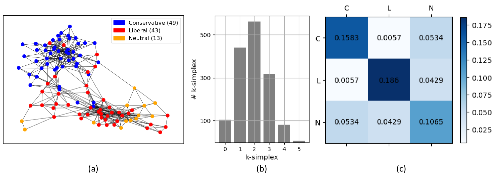
Figure 1: Configuration of the political book dataset. (a) indicates the data illustration using a graph, (b) presents the number of $k$-simplices, and (c) illustrates the connection probabilities between three labels: C (49 conservative books), L (43 liberal books), and N (13 neutral books).

In this study, we generate graphs using PPM in order to evaluate the proposed objective function in higher-order networks. First, a balanced graph is generated with $|I|=3$ and $|V|=150$, that is, there are 50 nodes corresponding to each label. The diagonal constant probability $p$ of the edge probability matrix $P$ is evaluated in the range $0.1\leq p\leq 0.2$, while the off diagonal probability constant $q$ is evaluated in $0.01\leq q\leq 0.025$. Furthermore, for semi-supervised node classification, the RW algorithm (as discussed in Section II-B) is employed as the initial probability distribution method over the nodes, and prior information ratio (the proportion of nodes whose labels are revealed) is assessed in the range from 0.01 to 0.10. Second, for an imbalanced graph with $|I|=3$ and $|V|=120$, the number of nodes corresponding to each label are set to be 60, 40, and 20. The initial probability distribution method as well as ranges of $p,q$, and prior information ratio remain consistent with the balanced experiment.

We utilize the co-purchase dataset of political books [35, 22] to further evaluate using a real dataset. The dataset captures the co-purchase records of 105 political books on Amazon during the 2004 U.S. president election period. Each book belongs to one of three labels: conservative (49 books), liberal (43 books), or neutral (13 books). Since edges represent frequent co-purchasing of books by the same buyers, this data set encapsulates various higher-order networks. It is noteworthy to report that the average connection probability between the same labeled nodes and different labeled nodes is 0.172 and 0.021, respectively. One node is chosen at random from each label and used as prior information, resulting in a prior information ratio of 0.029. The RW algorithm is also used for node initialization. The configuration of the data set is presented in Figure 1.

IV-B Optimization method

Sequential Quadratic Programming (SQP) [39, 40] is an iterative method used for constrained nonlinear optimization. The basic idea is to solve sequence of quadratic programming subproblems that approximates the original nonlinear problem. Each iteration of SQP refines the approximation and moves closer to the solution of the nonlinear problem. Sequential Least SQuare Programming (SLSQP) [41, 42], which is employed as our optimization method, is a variant of SQP, and it utilizes an approximate quadratic form of the objective function and constraints, transforming the problem into a constrained least square problem. SLSQP internally employs the quasi-Newton method to approximate the quadratic form of the objective function. This approach enhances efficiency by using an approximation instead of calculating the actual Hessian matrix (second derivative of the objective function.) It is known that SLSQP requires $O(n^{2})$ storage and $O(n^{3})$ time in $n$-dimensions [40].

IV-C Error metrics

Precision, Recall, F1-score, and Accuracy are employed as error metrics to evaluate the performance of the proposed objective function. In a multi-label classification, the concepts of the above error metrics remain fundamentally the same as in binary classification, but they can be computed for each label individually, that is, one vs rest. Let TP, TN, FP, and FN be the number of true positive, true negative, false positive, and false negative, respectively. Then the error metrics are defined by

Precision $$=\frac{TP}{TP+FP},$$

Recall $$=\frac{TP}{TP+FN},$$

F1-score $$=\frac{2*\text{\it Recall}*\text{\it Precision}}{\text{\it Recall}+\text{\it Precision}},$$

Accuracy $$=\frac{TP+FN}{TP+TN+FP+FN}.$$

In addition, Area Under Curve (AUC) is employed as an error metric. AUC denotes the area under the curve that plots the true positive rate (defined by TP/(TP+FN), that is Recall) against the false positive rate (defined by FP/(FP+TN)) at various threshold settings. AUC values of 1 and 0.5 indicate perfect classification and no better than random guessing of the algorithm, respectively.

V Results

In this section, we evaluate the node classification performance of the proposed higher-order networks-based method (5) on balanced generated data (Section V-A), imbalanced generated data (Section V-B), and imbalanced real data (political book data in Section V-C). We compare the performance of (5) (which we will call SI, standing for Simplicial Interactions) with the RW algorithm and with the following algorithm (PI), which uses an objective function involving only pairwise interactions

$$\text{Minimize }\,J_{2}\,\text{ over }\,\Delta^{n},\ \text{where }$$ (6)

$$J_{2}=\sum_{(j_{1},j_{2})\in K_{2}}\sum_{(i_{1},i_{2})=\theta\in S_{2}}C_{\theta}p_{i_{1}}^{j_{1}}p_{i_{2}}^{j_{2}}.$$

Problems (5) and (6) are both solved using RW for initialization, that is, the initial probability distribution $\{p_{i}^{j}\}_{i\in I,j\in V}$ is obtained as the solution (3) to the Dirichlet problem (2).

The evaluation is conducted on the ranges of $p,q$ and prior information ratio described in Section IV-A with respect to five error metrics AUC, Precision, Recall, F1-score, and Accuracy where $p,q$ indicates the constant probability of the edge probability matrix in PPM at on, off diagonal, respectively. Result summary and discussion is presented in Section V-D. The implementation algorithm can be found at https://github.com/kooeunho/HOI_objective.

V-A Balanced experiment

In this experiment, for the diagonal constant on and off probability $(p,q)$ of the edge probability matrix $P$ in PPM, three values of $p=0.10,0.15,0.20$ and four values of $q=0.010,0.015,0.020,0.025$ are tested. Also, the prior information ratio is tested with 0.01, 0.04, 0.07, and 0.10. Because the experiment selects the prior information (the nodes whose labels are exposed) randomly, we conduct 10 experiments for each value of $p,q$, and prior information ratio. Then the performance of the objective function is evaluated based on the averaged value of the 10 experiments with respect to the five error metrics. Overall averaged experimental result is presented in Figure 2.

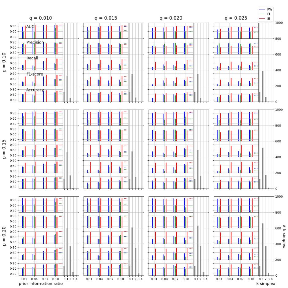
Figure 2: Experimental result on balanced generated graphs. The generated graphs consist of three labels, with 50 nodes for each label, totaling 150 nodes. Row and column correspond to homo-connection probability $p$ and hetero-connection probability $q$. Blue, green, and red indicate the performance with respect to AUC (first left plot in each panel), Precision (second), Recall (third), F1-score (fourth), and Accuracy (fifth). In each left panel, $x$-axis indicates the prior information ratio. Gray bars denote the number of $k$-simplices for each $p$ and $q$.

The result demonstrates that the performances of RW and PI are comparable. Thus, we primarily report the performance gain of the experiment applying SI in comparison to the mean performance of the RW and PI with respect to five error metrics in Figure 3.

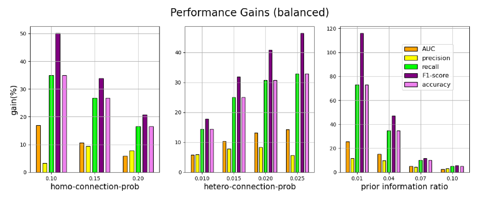
Figure 3: Performance gains of the balanced experiments applying SI in comparison to the mean performance of the RW and PI. Orange, yellow, lime, purple, and violet indicate AUC, Precision, Recall, F1-score, and Accuracy, respectively. Left, middle, and right correspond to the gains with respect to all candidates of homo-connection probability, hetero-connection probability, and prior information ratio, respectively.

There is a trend that the gains are greater when $p$ is lower, $q$ is higher, and the prior information ratio is lower, implying that SI obtains additional performance gains when the network structure information and the amount of prior information are unclear and limited.

V-B Imbalanced experiment

The hyperparameter setting ($p,q$ and prior information ratio) is the same as in the balanced experiment. Figure 4 depicts the overall averaged experimental result in terms of hyperparameters and five error metrics.

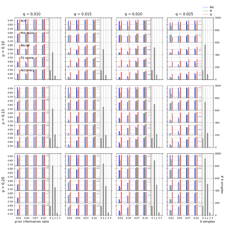
Figure 4: Experimental result on imbalanced generated graphs. The generated graphs consist of three labels, with 60,40, and 20, totaling 120 nodes. Row and column correspond to homo-connection probability $p$ and hetero-connection probability $q$. Blue, green, and red indicate the performance with respect to AUC (first left plot in each panel), Precision (second), Recall (third), F1-score (fourth), and Accuracy (fifth). In each left panel, $x$-axis indicates the prior information ratio. Gray bars denote the number of $k$-simplices for each $p$ and $q$.

Figure 5 depicts the performance gains.

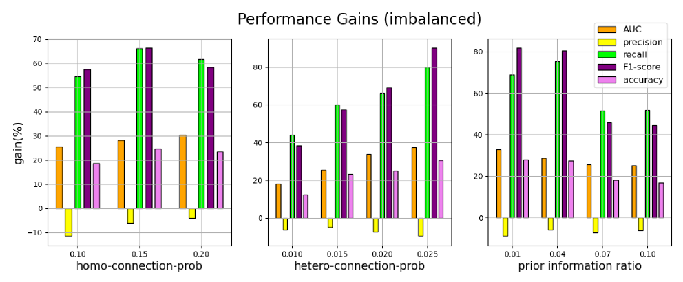
Figure 5: Performance gains of the imbalanced experiments applying SI in comparison to the mean performance of the RW and PI. Orange, yellow, lime, purple, and violet indicate AUC, Precision, Recall, F1-score, and Accuracy, respectively. Left, middle, and right correspond to the gains with respect to all candidates of homo-connection probability, hetero-connection probability, and prior information ratio, respectively.

The characteristic feature is that the results of experiments applying SI exhibit lower Precision and higher Recall compared to those using RW and PI. In essence, this means there are more false positives and less false negatives with SI. Such characteristics are critical when selecting algorithms for medical tests where, while there may be misidentifications of disease presence (false positives), missing an actual case (false negatives) can have serious consequences. In imbalanced experiments, we find that experiments using SI outperform experiments using RW and PI in accurately identifying labels corresponding to a minority of nodes, rather than classifying a majority of nodes under specific labels that encompass many nodes. When analyzing the results of many experiments involving imbalanced data, several factors come into play, such as the significance of minority labels and the balance between Precision and Recall. In these circumstances, the F1-score is frequently regarded as a reliable error metric [43]. The average percentage performance gain in F1-score for all hyperparameters in this experiment is 61.49 (Figure 5).

V-C Political books

As described in Section IV-A, the political book data set is imbalanced (49 conservative books, 43 liberal books, and 13 neutral books). For the semi-supervised experiment, one node is randomly chosen from each label, resulting in a prior information ratio of 0.029. The percentage performance gain of the SI compared to the mean performance of RW and PI with respect to AUC, Precision, Recall, F1-score, and Accuracy is found to be 29.18, 0.69, 105.04, 52.46, and 50.95, respectively (Figure 6(a)).

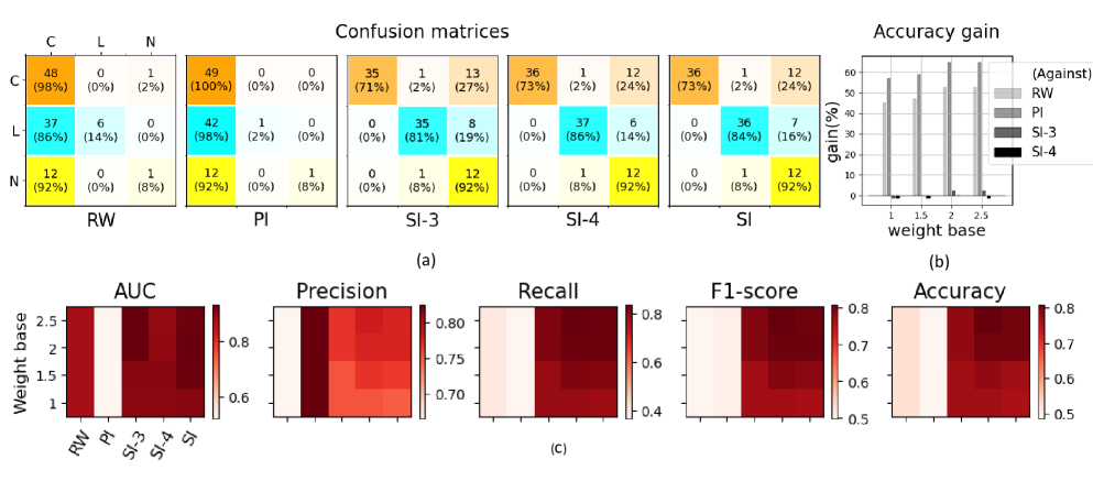
Figure 6: Experimental results on political book real dataset. (a) illustrates the performance change when applying up to $k$-simplices in the objective function as $k$ increases. (b) depicts the Accuracy gain when using SI (= SI-$6$) over RW, PI, SI-$3$, and SI-$4$ with varying weight parameter. (c) compares performance based on the weight base and the size of the applied simplices.

The trend of the gain being lower in Precision and higher in Recall and F1-score is consistent with the findings in Section V-B.

To fully investigate the fact that the political book data has 5-simplices as its maximal dimensional simplex, we evaluate the objective function’s performance using up to $K_{m}$ (the set of $(m-1)$-simplices in the graph) for each $m=2,3,4$, and $6$. That is, we also consider the following optimization

$$\text{Minimize }\,J_{m}\,\text{ over }\,\Delta^{n},\ \text{where }$$ (7)

$$J_{m}=\sum_{k=2}^{m}w_{k}\sum_{(j_{1},...,j_{k})\in K_{k}}\sum_{(i_{1},...,i_{k})=\theta\in S_{k}}C_{\theta}p_{i_{1}}^{j_{1}}p_{i_{2}}^{j_{2}}\dots p_{i_{k}}^{j_{k}},$$

and call it SI-m. Thus SI-$2$ = PI and SI-$6$ = SI. We omit SI-$5$ because the difference between SI-$5$ and SI-$6$ is expected to be small due to the scarcity of 5-simplices. In addition, for $w_{k}=\alpha^{k-1}$, we evaluate performance using $\alpha$-values of 1, 1.5, 2, and 2.5. In other words, we assess the performance of the objective function that assigns more weights as $k$ increases. The overall experimental results are shown in Figure 6(b),(c). The AUC performance gain of SI-$3$, SI-$4$, and SI over the mean performance of RW and PI is 30.94, 28.34, and 31.64, respectively. For Precision, 2.27, 3.53, and 3.12. For Recall, 110.16, 114.31, and 112.91. For F1-score and Accuracy, 55.53, 58.00, 57.19, and 53.78, 56.61, 55.19, respectively. It is found that the ratio of increase in performance gain diminishes considerably as $k$ increases. Furthermore, the performance gains of AUC for $\alpha=2.5$ against for $\alpha=1,1.5$, and $2$ is found to be 0.011, 0.004, and -0.002, respectively. For Precision, 0.019, 0.011, and 0.001. For Recall, 0.039, 0.022, and 0.002. For F1-score and Accuracy, 0.029, 0.016, 0.001, and 0.026, 0.020, 0.003, respectively. This result demonstrates that placing more weight on higher-order networks can be beneficial in achieving additional performance gains. It also shows that the weight is one of the important hyperparameters in the proposed higher-order networks-based objective function.

V-D Summary and discussion

We examined the performance of the proposed objective function (4) in a variety of contexts, including balanced, imbalanced, and political books datasets. Several notable experimental results and discussions are listed below.

First, it is evident that nodes corresponding to each label become more distinguishably separated in node classification tasks as the homo-connection probability ($p$) increases, the hetero-connection probability ($q$) decreases, and as the prior information ratio increases, facilitating community detection. However, the proposed function showed significant performance gains in the opposite scenario (lower $p$, higher $q$, and smaller prior information ratio) over all error metrics. This trend is consistent across both balanced and imbalanced experiments, implying the proposed objective function can be used in difficult classification settings, such as detecting overlapping communities.

Second, in imbalanced datasets (covering both generated and real data sets), experiments using all higher-order networks (dubbed SI) showed a performance gain with lower Precision but higher Recall and F1-score than the counterparts such as RW and PI. Because of this feature of the proposed objective function, it is applicable in many domains where precise classification of false negatives is critical, even if it comes at the cost of some false positives.

Third, according to the results from the political book real data, as we applied the objective function up to $K_{k}$ (the set of $(k-1)$-simplices in the graph), there is an improving trend as $k$ increases with respect to the five error metrics. However, this rate of growth showed diminishing returns. This implies that using all higher- order networks in the proposed objective function may be inefficient when compared to using up to a specific size of simplices. There is a need for research methodologies that select a small number of simplices while maintaining comparable node classification performance.

Fourth, increasing the weight parameter ($w_{k}$ in (4)) assigned to each $K_{k}$ as $k$ increases resulted in additional performance gain (Figure 6(b)). While this study used exponential weight parameters, further research into other types of weight parameters and their effects on performance is desired.

Fifth, the proposed objective function includes a domain constraint: the condition $\sum_{i=1}^{l}p_{i}^{j}=1$ must be satisfied, where $p_{i}^{j}$ denotes the probability of node $j$ having label $i$. Although there are ongoing neural network-based studies for optimizing objective functions with constraints [44], it is expected that when there are many nodes and labels, the number of parameters required for neural networks will be substantial. Because this study used the SLSQP optimization method without GPU acceleration, computational efficiency for large datasets with many nodes is limited. The development of neural network-based constrained optimization methodologies will be crucial for applying the proposed objective function to large real-world datasets.

Finally, for initialization in our node classification task (5), we used random walk and equilibrium measure-based Dirichlet boundary value approach. Many previous probability-based node classification studies focused on pairwise interactions or random walks, but they frequently overlooked higher-order interactions (HOI). Our findings show that when combined with HOI, the objective function can outperform in various PPM parameters when compared to the objectives relying solely on pairwise interactions. As a result, we believe that using previously trained node distributions from probability-based research as initial node distributions can improve performance when applying HOI to our proposed objective function.

VI Conclusion

In this paper, we propose a probability-based objective function for semi-supervised node classification that takes advantage of simplicial interactions of varying order. Given that densely connected nodes are likely to have similar properties, our proposed loss function imposes a greater penalty when nodes connected via higher-order simplices have diversified labels. For a given number of labels $l$, each node is equipped with an $l$-dimensional probability distribution. Using the Sequential Least SQuare Programming (SLSQP) optimization method, we seek the distribution across all nodes that minimizes the objective function under the constraint that the sum of node probabilities is one. Evaluations of our proposed function are carried out on balanced and imbalanced graphs generated using planted partition model (PPM), as well as on the political book real dataset. In challenging classification scenarios, where the probability of connections within the same label is low, the probability of connections between different labels is high, and there are fewer nodes with pre-known labels, incorporating higher-order networks into our proposed function outperforms results obtained by using only pairwise interactions or the random walk-based probabilistic method. Notably, while Precision is moderate for imbalanced data, both Recall and F1-score are significantly improved with our approach. This suggests potential applications in contexts like medical tests where minimizing false negatives, even at the expense of some false positives, is imperative. This study was framed within the optimization of functions with constraints, presenting a limitation: we cannot currently conduct GPU-based experiments, making it difficult to apply to real datasets with a large number of nodes. The advancement of research in neural network-based constrained optimization will allow us to apply our proposed objective function to large-scale real-world datasets, paving the way for future work.

References

- [1] S. Fortunato and D. Hric, “Community detection in networks: A user guide,” Physics reports, vol. 659, pp. 1–44, 2016.
- [2] M. T. Schaub, J.-C. Delvenne, M. Rosvall, and R. Lambiotte, “The many facets of community detection in complex networks,” Applied network science, vol. 2, no. 1, pp. 1–13, 2017.
- [3] P. Bonacich, A. C. Holdren, and M. Johnston, “Hyper-edges and multidimensional centrality,” Social networks, vol. 26, no. 3, pp. 189–203, 2004.
- [4] D. Easley, J. Kleinberg et al., Networks, crowds, and markets: Reasoning about a highly connected world. Cambridge university press Cambridge, 2010, vol. 1.
- [5] S. A. Marvel, J. Kleinberg, R. D. Kleinberg, and S. H. Strogatz, “Continuous-time model of structural balance,” Proceedings of the National Academy of Sciences, vol. 108, no. 5, pp. 1771–1776, 2011.
- [6] S. Klamt, U.-U. Haus, and F. Theis, “Hypergraphs and cellular networks,” PLoS computational biology, vol. 5, no. 5, p. e1000385, 2009.
- [7] A. R. Benson, D. F. Gleich, and D. J. Higham, “Higher-order network analysis takes off, fueled by classical ideas and new data,” arXiv preprint arXiv:2103.05031, 2021.
- [8] L. Torres, A. S. Blevins, D. Bassett, and T. Eliassi-Rad, “The why, how, and when of representations for complex systems,” SIAM Review, vol. 63, no. 3, pp. 435–485, 2021.
- [9] F. Battiston, G. Cencetti, I. Iacopini, V. Latora, M. Lucas, A. Patania, J.-G. Young, and G. Petri, “Networks beyond pairwise interactions: Structure and dynamics,” Physics Reports, vol. 874, pp. 1–92, 2020.
- [10] P. W. Holland, K. B. Laskey, and S. Leinhardt, “Stochastic blockmodels: First steps,” Social networks, vol. 5, no. 2, pp. 109–137, 1983.
- [11] D. Ghoshdastidar and A. Dukkipati, “Consistency of spectral partitioning of uniform hypergraphs under planted partition model,” Advances in Neural Information Processing Systems, vol. 27, 2014.
- [12] T. Lesieur, L. Miolane, M. Lelarge, F. Krzakala, and L. Zdeborová, “Statistical and computational phase transitions in spiked tensor estimation,” in 2017 IEEE International Symposium on Information Theory (ISIT). IEEE, 2017, pp. 511–515.
- [13] C. Kim, A. S. Bandeira, and M. X. Goemans, “Community detection in hypergraphs, spiked tensor models, and sum-of-squares,” in 2017 International Conference on Sampling Theory and Applications (SampTA). IEEE, 2017, pp. 124–128.
- [14] B. Karrer and M. E. Newman, “Stochastic blockmodels and community structure in networks,” Physical review E, vol. 83, no. 1, p. 016107, 2011.
- [15] T. P. Peixoto, “Hierarchical block structures and high-resolution model selection in large networks,” Physical Review X, vol. 4, no. 1, p. 011047, 2014.
- [16] S. Galhotra, A. Mazumdar, S. Pal, and B. Saha, “The geometric block model,” in Proceedings of the AAAI Conference on Artificial Intelligence, vol. 32, no. 1, 2018.
- [17] E. M. Airoldi, D. Blei, S. Fienberg, and E. Xing, “Mixed membership stochastic blockmodels,” Advances in neural information processing systems, vol. 21, 2008.
- [18] C. V. Cannistraci, G. Alanis-Lobato, and T. Ravasi, “From link-prediction in brain connectomes and protein interactomes to the local-community-paradigm in complex networks,” Scientific reports, vol. 3, no. 1, p. 1613, 2013.
- [19] M. E. Newman and M. Girvan, “Finding and evaluating community structure in networks,” Physical review E, vol. 69, no. 2, p. 026113, 2004.
- [20] V. D. Blondel, J.-L. Guillaume, R. Lambiotte, and E. Lefebvre, “Fast unfolding of communities in large networks,” Journal of statistical mechanics: theory and experiment, vol. 2008, no. 10, p. P10008, 2008.
- [21] X. Zhang and M. E. Newman, “Multiway spectral community detection in networks,” Physical Review E, vol. 92, no. 5, p. 052808, 2015.
- [22] M. E. Newman, “Modularity and community structure in networks,” Proceedings of the national academy of sciences, vol. 103, no. 23, pp. 8577–8582, 2006.
- [23] A. Vazquez, “Finding hypergraph communities: a bayesian approach and variational solution,” Journal of Statistical Mechanics: Theory and Experiment, vol. 2009, no. 07, p. P07006, 2009.
- [24] I. Chien, C.-Y. Lin, and I.-H. Wang, “Community detection in hypergraphs: Optimal statistical limit and efficient algorithms,” in International Conference on Artificial Intelligence and Statistics. PMLR, 2018, pp. 871–879.
- [25] D. Ghoshdastidar and A. Dukkipati, “Consistency of spectral hypergraph partitioning under planted partition model,” 2017.
- [26] E. Eaton and R. Mansbach, “A spin-glass model for semi-supervised community detection,” in Proceedings of the AAAI Conference on Artificial Intelligence, vol. 26, no. 1, 2012, pp. 900–906.
- [27] G. Ver Steeg, A. Galstyan, and A. E. Allahverdyan, “Statistical mechanics of semi-supervised clustering in sparse graphs,” Journal of Statistical Mechanics: Theory and Experiment, vol. 2011, no. 08, p. P08009, 2011.
- [28] A. E. Allahverdyan, G. Ver Steeg, and A. Galstyan, “Community detection with and without prior information,” Europhysics Letters, vol. 90, no. 1, p. 18002, 2010.
- [29] X. Ma, L. Gao, X. Yong, and L. Fu, “Semi-supervised clustering algorithm for community structure detection in complex networks,” Physica A: Statistical Mechanics and its Applications, vol. 389, no. 1, pp. 187–197, 2010.
- [30] Z.-Y. Zhang, “Community structure detection in complex networks with partial background information,” Europhysics Letters, vol. 101, no. 4, p. 48005, 2013.
- [31] Z.-Y. Zhang, K.-D. Sun, and S.-Q. Wang, “Enhanced community structure detection in complex networks with partial background information,” Scientific reports, vol. 3, no. 1, p. 3241, 2013.
- [32] D. Liu, X. Liu, W. Wang, and H. Bai, “Semi-supervised community detection based on discrete potential theory,” Physica A: Statistical Mechanics and its Applications, vol. 416, pp. 173–182, 2014.
- [33] K. Nowicki and T. A. B. Snijders, “Estimation and prediction for stochastic blockstructures,” Journal of the American statistical association, vol. 96, no. 455, pp. 1077–1087, 2001.
- [34] E. Bendito, A. Carmona, and A. M. Encinas, “Solving dirichlet and poisson problems on graphs by means of equilibrium measures,” European Journal of Combinatorics, vol. 24, no. 4, pp. 365–375, 2003.
- [35] O. L. V. Krebs, “http://www.orgnet.com/,” unpublished data.
- [36] C. Bick, E. Gross, H. A. Harrington, and M. T. Schaub, “What are higher-order networks?” SIAM Review, vol. 65, no. 3, pp. 686–731, 2023.
- [37] L.-H. Lim, “Hodge laplacians on graphs,” Siam Review, vol. 62, no. 3, pp. 685–715, 2020.
- [38] E. Abbe, “Community detection and stochastic block models: recent developments,” The Journal of Machine Learning Research, vol. 18, no. 1, pp. 6446–6531, 2017.
- [39] P. T. Boggs and J. W. Tolle, “Sequential quadratic programming,” Acta numerica, vol. 4, pp. 1–51, 1995.
- [40] J.-F. Bonnans, J. C. Gilbert, C. Lemaréchal, and C. A. Sagastizábal, Numerical optimization: theoretical and practical aspects. Springer Science & Business Media, 2006.
- [41] D. Kraft, “A software package for sequential quadratic programming,” Forschungsbericht- Deutsche Forschungs- und Versuchsanstalt fur Luft- und Raumfahrt, 1988.
- [42] ——, “Algorithm 733: Tomp–fortran modules for optimal control calculations,” ACM Transactions on Mathematical Software (TOMS), vol. 20, no. 3, pp. 262–281, 1994.
- [43] D. M. Powers, “Evaluation: from precision, recall and f-measure to roc, informedness, markedness and correlation,” arXiv preprint arXiv:2010.16061, 2020.
- [44] J. Chen and Y. Liu, “Neural optimization machine: A neural network approach for optimization,” arXiv preprint arXiv:2208.03897, 2022.