Cosmological Solutions of Chameleon Scalar Field Model

Abstract

We investigate cosmological solutions of the chameleon model with a non-minimal coupling between the matter and the scalar field through a conformal factor with gravitational strength. By considering the spatially flat FLRW metric and the matter density as a non-relativistic perfect fluid, we focus on the matter-dominated phase and the late-time accelerated-phase of the universe. In this regard, we manipulate and scrutinize the related field equations for the density parameters of the matter and the scalar fields with respect to the e-folding. Since the scalar field fluctuations depend on the background and the field equations become highly non-linear, we probe and derive the governing equations in the context of various cases of the relation between the kinetic and potential energies of the chameleon scalar field, or indeed, for some specific cases of the scalar field equation of state parameter. Thereupon, we schematically plot those density parameters for two different values of the chameleon non-minimal coupling parameter, and discuss the results. In the both considered phases, we specify that, when the kinetic energy of the chameleon scalar field is much less than its potential energy (i.e., when the scalar field equation of state parameter is $\simeq-1$), the behavior of the chameleon model is similar to the $\Lambda CDM$ model. Such compatibility suggests that the chameleon model is phenomenologically viable and can be tested with the observational data.

PACS number: 04.50.Kd; 98.80.-k; 04.20.Cv;
Keywords: Chameleon Scalar Field Model; Matter-Dominated Phase; Late-Time Accelerated-Phase

1 Introduction

It has been suggested that the universe starts from an extremely rapid accelerated-phase after the Planck era called the inflationary epoch that remedy important problems of the standard cosmological model (the $\Lambda CDM$ model), see, e.g., Refs. [1]-[7]. The cosmic microwave background observations are well consistent with the predictions of such an inflation hypothesis [8]. In the literature, a lot of work has been carried to investigate the inflationary scenario, see, e.g., Refs. [9]-[17]. After the inflationary epoch, observations predict that the universe has a decelerating era during the early phase of its evolution [18]. In fact, the universe undergoes a radiation dominated epoch followed by a matter dominated one. Afterward, the present accelerated-phase of the universe starts which is dubbed as a dark energy era. Indeed, observations – such as the type Ia supernova, the baryon acoustic oscillations, and the gravitational waves – confirm the late-time cosmic acceleration [8, 18]-[25]. But the driver of such acceleration has not been identified by observations and has no fully accepted theoretical model. However, since ordinary matter cannot accelerate the universe, such dark energy (if it exists) must be exotic matter for which many candidates have been proposed and investigated. In most of these models, a scalar field has been employed as dark sector with a dynamical equation of state. On the other hand, modified gravitational theories (e.g. Refs. [26]-[41] and references therein) have also been proposed mainly to describe the accelerated evolution of the universe without any sector as dark energy. For these two issues see, e.g., Refs. [42]-[60] and references therein. Furthermore, other observations – such as the behavior of the galactic rotation curves and the mass discrepancy in clusters of galaxies – indicate the consideration of an exotic matter called dark matter [61]-[64]. A lot of alternative efforts have also been performed on various modifications to the Einstein field equations in order to deal with the question of dark matter [45, 47, 65]-[71] and references therein. Howsoever, the nature of both of these dark sectors (which constitute about $95\%$ of the universe [8, 18] and are well consistent with the observational data [72]) is one of the most important issues in physics.

Although general relativity provides accurate predictions in describing some cosmological phenomena [73], the $\Lambda$CDM is the most acceptable model due to its high conformity with the observational data of cosmology [74]. However, this model still confronts some challenges [75]-[83] and other alternatives have been proposed for it. The scalar-tensor theories of gravitation, which extend general relativity by introducing a scalar field, have become the most popular alternative to the Einstein gravitational theory [84]-[94].

In this work, we concentrate on the chameleon scalar field theory, wherein unlike the common non-minimally coupled scalar field theories, a chameleon field couples with matter sector rather than the geometry. Such an interaction between the scalar field and matter field causes the effective potential of the scalar field depends on the matter density of the environment. Much work has been done on this theory, see, e.g., Refs. [10, 37, 59, 95]-[113] and references therein. This change of properties of the mass of scalar field acts as a buffer with respect to observational bounds. Accordingly, in this type of theory, a screening mechanism is usually aimed at modifying general relativity on large scales. Hence, the chameleon scalar field theory can be employed to describe the accelerated expansion of the universe while the effects of non-minimal coupling parameter are hidden in the small scale gravitational experiments, see, e.g., Refs. [95]-[98, 101, 102].

We have previously investigated the chameleon model during inflation in Refs. [10, 107], wherein we showed through the proposed scenario that the effects of inflation and chameleon can be described via a single scalar field during the inflation and late-time. Also, we have probed the role of the chameleon scalar field as dark energy in Ref. [59], where it was claimed that such a model justifies dark energy with stronger confirmation. Now, in this work, we intend to investigate the cosmological solutions of the chameleon model in the hope that these solutions can better justify the observational data. Of course, since in the chameleon model, the properties of the scalar fluctuations depend on the background, its field equations of motion become highly non-linear. However, rather than solving the resulted equations analytically, we restrict the solutions to proceed. Indeed, for various cases of the relation between the kinetic and potential energies of the chameleon scalar field (or actually, for some specific cases of the scalar field equation of state parameter), we solve the non-minimal coupled gravity equations to understand the evolution of the scalar field. Meanwhile, some attempts have been done to find analytic solutions for the chameleon model, wherein these analytic solutions of the chameleon model exist only for highly symmetric source shapes such as spheres, plates, and ellipses [95, 114, 115]). If the shape of the matter source is irregular, it will be more difficult to find analytical solutions to the equations of motion. Nevertheless, in Ref. [116], a software package called SELCIE has been introduced that provides tools for constructing an arbitrary system of mass distributions and then computing the corresponding solution to the chameleon scalar field equation. In addition, through the dynamical systems technique [117, 118], one can also study the full non-linearity of these cosmological models. In this technique, usually normalized dimensionless new variables are introduced, then by finding the fixed/critical points of the system and their stability, the evolution of the system can be pictured qualitatively near these points. The dynamical systems technique has also been performed for the chameleon scalar field, see, e.g., Refs. [100, 103, 105, 112].

The work is organized as follows. In the next two sections, while benefiting from our previous works [10, 59, 107], we first introduce the chameleon model and then, by considering the spatially flat Friedmann-Lemaître-Robertson-Walker (FLRW) metric, we obtain the corresponding field equations of motion. Thereupon, in Sec. III, we manipulate and scrutinize the related field equations with respect to the e-folding for better and more use in the later sections. In Secs. IV and V, the cosmological solutions of the chameleon model are respectively investigated for the matter-dominated phase and the late-time accelerated-phase of the universe for various cases of the relation between the kinetic and potential energies of the chameleon scalar field. Indeed, we probe the results of the chameleon model for some specific cases of the scalar field equation of state parameter. Meanwhile, in Sec. V, we take a brief look at the chameleon scalar field profile. At last, we conclude the work in Sec. VI with the summary of the results.

2 Chameleon Model with Scalar Field

We consider an action of the chameleon model with a scalar field in four dimensions when there are a minimal coupling between the Einstein gravity and that scalar field, and a non-minimal coupling between matter species with it as

$$S\!\!\! =\!\!\! \!\!\int{\rm d}^{4}x\sqrt{-g}\left(\frac{M^{2}_{\rm Pl}R}{2}\right)\!-\!\!\!\int{\rm d}^{4}x\sqrt{-g}\left[\frac{1}{2}\partial_{\mu}\phi\partial^{\mu}\phi+V(\phi)\right]$$ (1)

$$+\sum_{i}\int{\rm d}^{4}x\sqrt{-{\tilde{g}}_{(i)}}{L_{(i)}^{\rm(m)}}\left({\psi}_{(i)}^{\rm(m)},{\tilde{g}}_{(i)\mu\nu}\right).$$

In this action, $\phi$ is a scalar field, $V(\phi)$ is a self-interacting potential, $\psi_{(i)}$s are various matter fields, ${L^{\rm(m)}_{(i)}}$s are Lagrangians of matter fields, $\tilde{g}_{(i)\mu\nu}$s are matter field metrics that are conformally related to the Einstein frame metric as

$${\tilde{g}}_{(i)\mu\nu}={e}^{{2\frac{{\beta}_{(i)}\,\phi}{M_{\rm Pl}}}}{g}_{\mu\nu}.$$ (2)

Here, $\beta_{(i)}$s are dimensionless constants that represent different non-minimal coupling parameter between the scalar field and each matter species, however in this work, we only consider a single matter component. Also, the lower case Greek indices run from zero to three, $g$ is the determinant of the metric, $R$ is the Ricci scalar, and the reduced Planck mass is $M_{\rm Pl}\equiv(8\pi G)^{-1/2}\approx 10^{27}eV$ in the natural units of $\hbar=1=c$. Typically in the literature, the common power-law chameleon potential

$$V\left(\phi\right)=\frac{{{M^{4+n}}}}{{{\phi^{n}}}}$$ (3)

is usually used, where $n$ is a positive or negative integer constant and $M$ is some positive constant mass scale.

The variation of action (1) with respect to the scalar field gives the field equation

$$\Box\phi=\frac{{dV\left(\phi\right)}}{{d\phi}}-\frac{{\beta}}{M_{\rm Pl}}e^{4\frac{{\beta}\phi}{{M}_{\rm Pl}}}{\tilde{g}}^{\mu\nu}{\tilde{T}}_{\mu\nu}^{(m)},$$ (4)

where the box symbol $\Box\equiv\nabla^{\alpha}\nabla_{\alpha}$ corresponds to the metric $g_{\mu\nu}$, and $\tilde{T}_{\mu\nu}^{(m)}$ is the energy-momentum tensor of matter (which is conserved in the Jordan frame) defined as

$$\tilde{T}_{\mu\nu}^{(m)}=-\frac{2}{\sqrt{-\tilde{g}}}\frac{\left(\delta{\sqrt{-\tilde{g}}}{L^{(m)}}\right)}{\delta{\tilde{g}}^{\mu\nu}}.$$ (5)

Also, the variation with respect to the metric $g_{\mu\nu}$ associated to the Einstein frame gives

$${G_{\mu\nu}}=\frac{1}{M_{\rm Pl}^{2}}\left(T_{\mu\nu}^{(\phi)}+T_{\mu\nu}^{(m)}\right)=\frac{1}{M_{\rm Pl}^{2}}\left(T_{\mu\nu}^{(\phi)}+{e}^{{2\frac{{\beta}\phi}{M_{\rm Pl}}}}\tilde{T}_{\mu\nu}^{(m)}\right),$$ (6)

where $T_{\mu\nu}^{(\phi)}$ is the energy-momentum tensor of the scalar field as

$$T_{\mu\nu}^{(\phi)}=-\frac{1}{2}{g_{\mu\nu}}{\partial^{\alpha}}\phi{\partial_{\alpha}}\phi-{g_{\mu\nu}}V\left(\phi\right)+{\partial_{\mu}}\phi{\partial_{\nu}}\phi.$$ (7)

In addition, we assume the matter field as a perfect fluid in the Jordan frame with the linear barotropic equation of state $\tilde{p}^{(m)}=w\tilde{\rho}^{(m)}$. Hence, one obtains the trace of the energy-momentum tensor (5), with the signature $+2$, as

$$\tilde{T}^{(m)}={\tilde{g}}^{\mu\nu}\tilde{T}_{\mu\nu}^{(m)}=-(1-3w)\tilde{\rho}^{(m)},$$ (8)

where the relation between the matter density in the Einstein frame with the Jordan frame is

$$\rho^{(m)}=e^{4\frac{{\beta}\phi}{M_{\rm Pl}}}\tilde{\rho}^{(m)}.$$ (9)

The matter density $\tilde{\rho}^{(m)}$ is conserved in the Jordan frame, i.e.

$$\dot{\tilde{\rho}}^{(m)}+3\tilde{H}\left(1+w\right)\tilde{\rho}^{(m)}=0,$$ (10)

however, it is not conserved in the Einstein frame. Nevertheless, the mathematical quantity

$$\rho(t)\equiv e^{3(1+w)\frac{{\beta}\phi}{M_{\rm Pl}}}\tilde{\rho}^{(m)},$$ (11)

independent of the scalar field and with the same equation of state parameter, is a conserved quantity in this frame, i.e.

$$\dot{\rho}+3H\left(1+w\right)\rho=0.$$ (12)

Of course, this $\rho(t)$ is not a physical matter density. Furthermore, substituting definition (11) into Eq. (4) yields the dynamic of the scalar field governed by an effective potential, i.e.

$$\Box\phi=\frac{{d{V_{\rm eff}}\left(\phi\right)}}{{d\phi}},$$ (13)

where

$${V}_{\rm eff}(\phi)\equiv V(\phi)+\rho e^{(1-3w)\frac{\beta\phi}{M_{\rm Pl}}}=V(\phi)+\rho^{(m)},$$ (14)

which depends explicitly on the matter density. Additionally, the mass of the chameleon field, which is sufficiently large to evade local constraints [95, 120], is

$$m_{\rm eff,\min}^{2}={V^{\prime\prime}_{\rm eff}}\left({{\phi_{\min}}}\right)=V^{\prime\prime}\left({{\phi_{\min}}}\right)+\frac{{{\beta^{2}}}}{{M_{\rm Pl}^{2}}}{\left({1-3w}\right)^{2}}\rho{e^{\frac{{\beta{\phi_{\min}}}}{{{M_{\rm Pl}}}}}}.$$ (15)

In the following, we derive the relevant field equations in order to investigate the cosmology of such a chameleon model.

3 Scrutinizing Field Equations

In this section, we intend to manipulate and scrutinize the cosmological equations of the chameleon model while considering the spatially flat FLRW metric in the Einstein frame, namely

$$ds^{2}=-dt^{2}+a^{2}(t)\left(dx^{2}+dy^{2}+dz^{2}\right),$$ (16)

where $a(t)$ is the scale factor as a function of the cosmic time $t$. In this respect, first, the field equation (13) gives the wave equation

$$\ddot{\phi}+3H\dot{\phi}+\frac{{d{V_{\rm eff}}\left(\phi\right)}}{{d\phi}}=0,$$ (17)

where we have also considered the scalar field just as a function of the cosmic time, dot denotes the derivative with respect to this time, and $H(t)\equiv\dot{a}/a$ is the Hubble parameter. Furthermore by metric (16), Eq. (6) gives the corresponding Friedmann and Raychaudhuri equations as

$${H^{2}}=\frac{1}{3{M_{\rm Pl}^{2}}}\left({\frac{1}{2}{{\dot{\phi}}^{2}}+V\left(\phi\right)+\rho{e^{\left({1-3w}\right)\frac{{\beta\phi}}{{{M_{\rm Pl}}}}}}}\right)$$ (18)

and

$$-M^{2}_{\rm Pl}\left(\frac{2\ddot{a}}{a}+H^{2}\right)=\frac{1}{2}\dot{\phi}^{2}-V(\phi)+w\rho e^{\left(1-3w\right)\frac{\beta\phi}{M_{\rm Pl}}}.$$ (19)

Also, relation (7) gives the energy and the pressure densities as

$${\rho^{\left(\phi\right)}}=\frac{1}{2}{{\dot{\phi}}^{2}}+V\left(\phi\right)\qquad{\rm and}\qquad{p^{\left(\phi\right)}}=\frac{1}{2}{{\dot{\phi}}^{2}}-V\left(\phi\right).$$ (20)

Accordingly, Eqs. (18) and (19) can be rewritten as

$${H^{2}}=\frac{1}{{3M_{\rm Pl}^{2}}}\left({{\rho^{\left(\phi\right)}}+{\rho^{\left(m\right)}}}\right)=\frac{1}{{3M_{\rm Pl}^{2}}}{\rho^{\left({\rm tot}\right)}},$$ (21)

$$\frac{{\ddot{a}}}{a}=-\frac{1}{{6M_{\rm Pl}^{2}}}\left[{{\rho^{\left(\phi\right)}}+{\rho^{\left(m\right)}}+3\left({{p^{\left(\phi\right)}}+{p^{\left(m\right)}}}\right)}\right]=-\frac{1}{{6M_{\rm Pl}^{2}}}\left({{\rho^{\left({\rm tot}\right)}}+3{p^{\left({\rm tot}\right)}}}\right),$$ (22)

where $\rho^{(\rm tot)}\equiv\rho^{(\phi)}+\rho^{(m)}$ and $p^{(\rm tot)}\equiv p^{(\phi)}+p^{(m)}$ are the total energy and pressure densities. The field equations (21) and (22) indicate that $\rho^{(\rm tot)}$ is conserved in the Einstein frame, i.e.

$${\dot{\rho}}^{(\rm tot)}+3H\left(\rho^{(\rm tot)}+p^{(\rm tot)}\right)=0.$$ (23)

However, in general, the scalar and matter fields are not separately conserved in this frame, and an interacting term stands among those, i.e.

$${\dot{\rho}}^{(m)}+3H\left(\rho^{(m)}+p^{(m)}\right)=\frac{\beta\left(1-3w\right)}{M_{\rm Pl}}\rho^{(m)}\dot{\phi}$$ (24)

and

$${\dot{\rho}}^{(\phi)}+3H\left(\rho^{(\phi)}+p^{(\phi)}\right)=-\frac{\beta\left(1-3w\right)}{M_{\rm Pl}}\rho^{(m)}\dot{\phi},$$ (25)

wherein the interacting term depends on the scalar field and the background matter density of the environment. However, for an ultra-relativistic matter, with $w=1/3$, such an interacting term is identically zero. That is, for the radiation dominated epoch of the universe, the scalar and matter fields are separately conserved.

In the following analysis, we consider the matter density as a non-relativistic perfect fluid, i.e. dust matter with $w=0$. Accordingly, Eqs. (24) and (25) read

$${\dot{\rho}}^{(m)}+3H\rho^{(m)}=\frac{\beta}{M_{\rm Pl}}\rho^{(m)}\dot{\phi}$$ (26)

and

$${\dot{\rho}}^{(\phi)}+3H{\rho^{(\phi)}}\left({1+{w^{(\phi)}}}\right)=-\frac{\beta}{M_{\rm Pl}}\rho^{(m)}\dot{\phi},$$ (27)

where ${w^{(\phi)}}=p^{(\phi)}/\rho^{(\phi)}$. Moreover, we present the equations via the dimensionless density parameters defined as

$${\Omega^{(m)}}\equiv\frac{\rho^{(m)}}{{\rho_{0}^{\rm(crit)}}}\qquad{\rm and}\qquad{\Omega^{(\phi)}}\equiv\frac{{{\rho^{(\phi)}}}}{{\rho_{0}^{\rm(crit)}}},$$ (28)

where $\rho_{0}^{\rm(crit)}\equiv 3H_{0}^{2}M_{\rm Pl}^{2}$ is the critical density of the universe at the present-time. Hence, Eq. (21) can be rewritten as

$${H^{2}}=H_{0}^{2}\left[{{\Omega^{(\phi)}}+{\Omega^{(m)}}}\right],$$ (29)

which in turn imposes constraint

$${\Omega_{0}^{(\phi)}}+{\Omega_{0}^{(m)}}=1$$ (30)

on the initial values at the present-time.

On the other hand, by employing the e-folding variable

$$N=\ln\left[{\frac{{a(t)}}{{a({t_{0}})}}}\right],$$ (31)

we have

$$\frac{d}{{dt}}=H\frac{d}{{dN}}.$$ (32)

Also from relations (20) and (28), we obtain

$$\dot{\phi}=\pm\sqrt{{\rho^{\left(\phi\right)}}+{p^{\left(\phi\right)}}}=\pm{H_{0}}{M_{\rm Pl}}\sqrt{3{\Omega^{(\phi)}}\left({1+{w^{(\phi)}}}\right)}.$$ (33)

It has been shown [120] that the monotonic increase of the matter coupling factor ${e^{\frac{{\beta\phi}}{{{M_{\rm Pl}}}}}}$, when corresponds to $\dot{\phi}>0$, leads to a minimum for ${V_{\rm eff}}\left(\phi\right)$. Moreover, It has been stated [121] that $\dot{\phi}>0$ is satisfactory from the astrophysical point of view [122]. Hence, we confine our investigation to the positive sign in relation (33) to proceed, and the generalization to the negative sign can be performed with similar considerations. Thus, Eqs. (26) and (27) read

$${\Omega^{\prime}}^{(m)}+3{\Omega^{(m)}}=\frac{{\beta{H_{0}}}}{H}{\Omega^{(m)}}\sqrt{3{\Omega^{(\phi)}}\left(1+w^{(\phi)}\right)}$$ (34)

and

$${{\Omega^{\prime}}^{(\phi)}}+3{\Omega^{(\phi)}}\left({1+{w^{(\phi)}}}\right)=-\frac{{\beta{H_{0}}}}{H}{\Omega^{(m)}}\sqrt{3{\Omega^{(\phi)}}\left({1+{w^{(\phi)}}}\right)},$$ (35)

where the prime denotes the derivative with respect to the e-folding.

In addition, in the case of $w=0$, the defined total equation of state parameter for this model is

$${w^{\left({\rm tot}\right)}}\equiv\frac{{{p^{\left({\rm tot}\right)}}}}{{{\rho^{\left({\rm tot}\right)}}}}=\frac{{{p^{\left(\phi\right)}}}}{{{\rho^{\left(m\right)}}+{\rho^{\left(\phi\right)}}}}.$$ (36)

Also, using the deceleration parameter, i.e. $q\equiv-{\ddot{a}}a/{\dot{a}}^{2}=-{\ddot{a}}/(aH^{2})$, while substituting Eqs. (21) and (22), with employing the definition of the total equation of state parameter, into it, leads to

$$q=\frac{{1+3{w^{\left({\rm tot}\right)}}}}{2}.$$ (37)

Obviously if $q<0$ (which is equal to ${w^{\left({\rm tot}\right)}}<-1/3$), it will describe an accelerated-phase in evolution of the universe.

In the continuation of the work, we intend to investigate the cosmological solutions of the chameleon model for two important phases of the cosmos.

4 Matter-Dominated Phase

Under assumption ${\rho^{\left(m\right)}}\gg{\rho^{\left(\phi\right)}}$, which corresponds to ${\Omega^{(m)}}\gg{\Omega^{(\phi)}}$, the total equation of state parameter (36) yields

$${w^{\left({\rm tot}\right)}}\simeq\frac{{{p^{\left(\phi\right)}}}}{{{\rho^{\left(m\right)}}}}.$$ (38)

Now, if the chameleon potential $V\left(\phi\right)$ being positive, then relations (20) will indicate that ${p^{\left(\phi\right)}}<{\rho^{\left(\phi\right)}}$, and in turn ${\rho^{\left(m\right)}}\gg{p^{\left(\phi\right)}}$, hence relation (38) gives

$${w^{\left({\rm tot}\right)}}\simeq 0,$$ (39)

for the matter density as a non-relativistic perfect fluid. Furthermore, in this situation, the deceleration parameter (37) is

$$q\simeq\frac{1}{2},$$ (40)

i.e. the expansion of the universe is a decelerated evolution.

On the other hand, in the matter-dominated phase, Eq. (21) reduces to

$${H^{2}}\simeq H_{0}^{2}{\Omega^{(m)}},$$ (41)

and hence, Eqs. (34) and (35) read

$${\Omega^{\prime}}^{(m)}+3{\Omega^{(m)}}\simeq\beta\sqrt{3\Omega^{(m)}\,\,{\Omega^{(\phi)}}{\left({1+{w^{(\phi)}}}\right)}}$$ (42)

and

$${{\Omega^{\prime}}^{(\phi)}}+3{\Omega^{(\phi)}}\left({1+{w^{(\phi)}}}\right)\simeq-\beta\sqrt{3\Omega^{(m)}\,\,{\Omega^{(\phi)}}{\left({1+{w^{(\phi)}}}\right)}}.$$ (43)

In the above, one obviously has $\rho^{(m)}>0$ and $H>0$, wherein we have assumed that $\rho^{(\phi)}>0$, i.e. ${\dot{\phi}}^{2}/2>\mid V(\phi)\mid$ for negative potentials. Also, we have assumed that

$${w^{(\phi)}}\geq-1,$$ (44)

which, with relations (20) and the assumption $\rho^{(\phi)}>0$, it is already satisfied.

At this stage, it is more instructive to define two new parameters $y\equiv\sqrt{{\Omega^{\left(m\right)}}}$ and $x\equiv\sqrt{{\Omega^{\left(\phi\right)}}}$. Thus, we can rewrite Eqs. (42) and (43) as the following coupled first derivative equations for $x$ and $y$, namely

$$2y^{\prime}+3y\simeq\beta x\sqrt{3{\left({1+{w^{(\phi)}}}\right)}}$$ (45)

and

$$2x^{\prime}+3x{\left({1+{w^{(\phi)}}}\right)}\simeq-\beta y\sqrt{3{\left({1+{w^{(\phi)}}}\right)}}.$$ (46)

However, rather than solving these coupled equations analytically, we restrict the solutions to proceed. Indeed, in the following subsections, we investigate the solutions of these coupled differential equations for various cases of the relation between the kinetic and potential energies of the chameleon scalar field. Actually, we probe the results of the chameleon model for four specific cases of the scalar field equation of state parameter.

4.1 Case ${\dot{\phi}^{2}}/2\gg\mid V\left(\phi\right)\mid$

In this case, one obviously has ${w^{\left(\phi\right)}}\simeq+1$, hence Eqs. (45) and (46) read

$$2y^{\prime}+3y\simeq\sqrt{6}\,\beta x,$$ (47)

$$2x^{\prime}+6x\simeq-\sqrt{6}\,\beta y.$$ (48)

Now, by applying the upper bound value of the $\beta=3.7\times{10^{2}}$ (which this value of the non-minimal coupling parameter in the chameleon model has been shown [123] to be consistent with the experimental constrain), the solutions of these equations are

$$y\left(N\right)=-\frac{{{e^{-\frac{9}{4}N}}}}{{1480}}\Bigg{[}\!\!\!\!\! \Big{(} \!\!\!\!\!{C_{1}}\sqrt{6}-{C_{2}}\sqrt{2190394}\Big{)}\sin\left({\frac{{\sqrt{3285591}}}{4}N}\right)$$ (49)

$$+ \!\!\!\!\!\left({{C_{1}}\sqrt{2190394}+{C_{2}}\sqrt{6}}\right)\cos\left({\frac{{\sqrt{3285591}}}{4}N}\right)\Bigg{]}$$ (50)

and

$$x\left(N\right)={e^{-\frac{9}{4}N}}\left[{{C_{1}}\sin\left({\frac{{\sqrt{3285591}}}{4}N}\right)+{C_{2}}\cos\left({\frac{{\sqrt{3285591}}}{4}N}\right)}\right],$$ (51)

where $C_{1}$ and $C_{2}=x(0)$ are constants of integrations. Using solutions (49) and (51), we have plotted ${\Omega^{\left(m\right)}}={y^{2}}$ and ${\Omega^{\left(\phi\right)}}={x^{2}}$ in Figure 1, wherein (without loss of generality) the present values of the parameters have been used to specify the constants. This figure indicates that the behavior of the matter density and the chameleon scalar field density are both damped oscillations, i.e. the value of both densities decreases over time. Note that, the negative values of the e-folding in this figure (and also in the subsequent figures) are because we have assumed the value of the scale factor to be equal to one at the present-time, i.e. ${a({t_{0}})}=1$. We should also remind that the zero values of ${\Omega^{\left(m\right)}}$ and ${\Omega^{\left(\phi\right)}}$ must be disregarded in all the figures.

On the other hand, by considering the non-minimal coupling parameter as $\beta=1$, Eqs. (47) and (48) lead to solutions

$$y\left(N\right)=-\frac{{e^{-\frac{9}{4}N}}}{4}\left[{\left({{C_{3}}\sqrt{6}-{C_{4}}\sqrt{10}}\right)\sin\left({\frac{{\sqrt{15}}}{4}N}\right)+\left({{C_{3}}\sqrt{10}+{C_{4}}\sqrt{6}}\right)\cos\left({\frac{{\sqrt{15}}}{4}N}\right)}\right]$$ (52)

and

$$x\left(N\right)={e^{-\frac{9}{4}N}}\left[{{C_{3}}\sin\left({\frac{{\sqrt{15}}}{4}N}\right)+{C_{4}}\cos\left({\frac{{\sqrt{15}}}{4}N}\right)}\right],$$ (53)

where $C_{3}$ and $C_{4}=x(0)$ are constants of integrations. Also, using solutions (52) and (53), we have plotted ${\Omega^{\left(m\right)}}$ and ${\Omega^{\left(\phi\right)}}$ in Figure 2. This figure indicates that at the beginning of this phase of the universe the matter density dominates, and then at the end of its dominance era, the chameleon scalar field density is dominant.

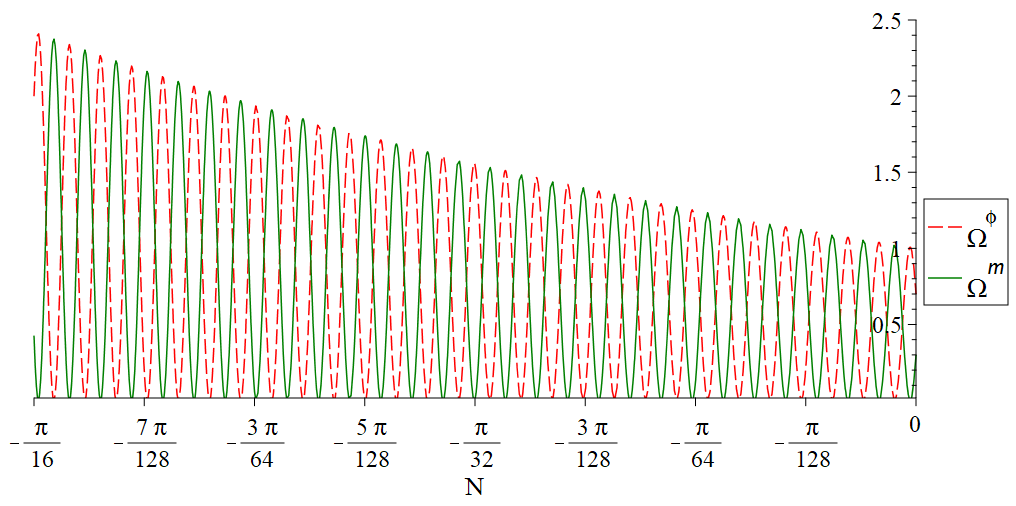
Figure 1: For solutions (49) and (51) with $\beta=3.7\times{10^{2}}$, the figure schematically (i.e., scale-free) shows the parameters ${\Omega^{\left(m\right)}}$ and ${\Omega^{\left(\phi\right)}}$ versus $N$ as solid and dashed lines, respectively. Besides, the present values of the parameters, i.e. $\Omega^{(m)}_{0}\simeq{0.3}$ and ${\Omega^{(\phi)}_{0}}\simeq{0.7}$ (the current observational data for all matter is up to $32\%$ and for dark energy roughly $68\%$ of the universe [18]), have been used as the initial conditions, and ${a({t_{0}})}=1$.

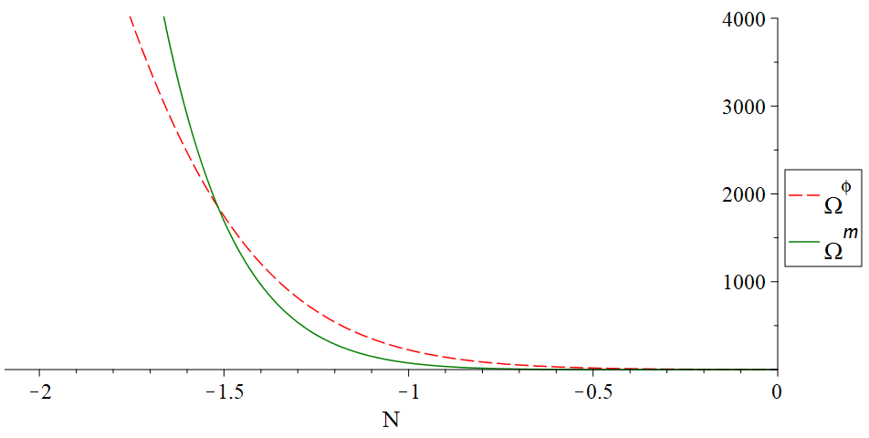
Figure 2: For solutions (52) and (53) with $\beta=1$, the figure schematically (i.e., scale-free) shows the parameters ${\Omega^{\left(m\right)}}$ and ${\Omega^{\left(\phi\right)}}$ versus $N$ as solid and dashed lines, respectively. Besides, the present values of the parameters, i.e. $\Omega^{(m)}_{0}\simeq{0.3}$ and ${\Omega^{(\phi)}_{0}}\simeq{0.7}$, have been used as the initial conditions, and ${a({t_{0}})}=1$.

4.2 Case ${\dot{\phi}^{2}}/2=V\left(\phi\right)$

In this case, the chameleon potential must be positive, and accordingly relations (39) and (40) will hold. In addition, one gets ${w^{\left(\phi\right)}}=0$, hence Eqs. (45) and (46) read

$$2y^{\prime}+3y\simeq\sqrt{3}\,\beta x,$$ (54)

$${}\quad 2x^{\prime}+3x\simeq-\sqrt{3}\,\beta y.$$ (55)

The solutions to these equations with $\beta=3.7\times{10^{2}}$ are

$$y\left(N\right)=-{e^{-\frac{3}{2}N}}\left[{{C_{5}}\cos\left({185\sqrt{3}N}\right)-{C_{6}}\sin\left({185\sqrt{3}N}\right)}\right]$$ (56)

and

$$x\left(N\right)={e^{-\frac{3}{2}N}}\left[{{C_{5}}\sin\left({185\sqrt{3}N}\right)+{C_{6}}\cos\left({185\sqrt{3}N}\right)}\right],$$ (57)

where $C_{5}=-y(0)$ and $C_{6}=x(0)$ are constants of integrations. Using solutions (56) and (57), we have plotted ${\Omega^{\left(m\right)}}$ and ${\Omega^{\left(\phi\right)}}$ in Figure 3.

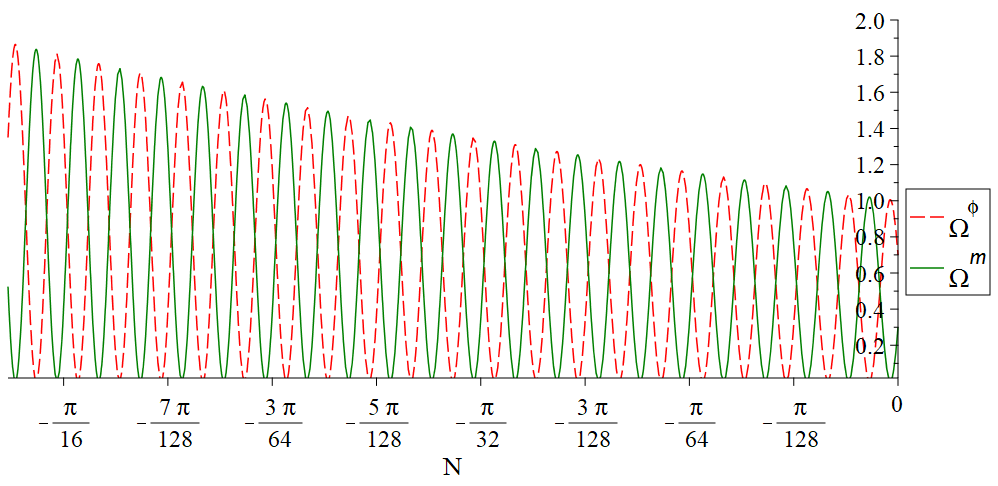
Figure 3: For solutions (56) and (57) with $\beta=3.7\times{10^{2}}$, the figure schematically (i.e., scale-free) shows the parameters ${\Omega^{\left(m\right)}}$ and ${\Omega^{\left(\phi\right)}}$ versus $N$ as solid and dashed lines, respectively. Besides, the present values of the parameters, i.e. $\Omega^{(m)}_{0}\simeq{0.3}$ and ${\Omega^{(\phi)}_{0}}\simeq{0.7}$, have been used as the initial conditions, and ${a({t_{0}})}=1$.

This figure indicates that the behavior of the matter density and the chameleon scalar field density are both also damped oscillations and their values decrease over time.

However, using the non-minimal coupling parameter $\beta=1$, Eqs. (54) and (55) lead to

$$y\left(N\right)=-{e^{-\frac{3}{2}N}}\left[{{C_{7}}\cos\left({\frac{{\sqrt{3}}}{2}N}\right)-{C_{8}}\sin\left({\frac{{\sqrt{3}}}{2}N}\right)}\right]$$ (58)

and

$$x\left(N\right)={e^{-\frac{3}{2}N}}\left[{{C_{7}}\sin\left({\frac{{\sqrt{3}}}{2}N}\right)+{C_{8}}\cos\left({\frac{{\sqrt{3}}}{2}N}\right)}\right],$$ (59)

where $C_{7}=-y(0)$ and $C_{8}=x(0)$ are constants of integrations. Again, we have plotted ${\Omega^{\left(m\right)}}$ and ${\Omega^{\left(\phi\right)}}$ from solutions (58) and (59) in Figure 4.

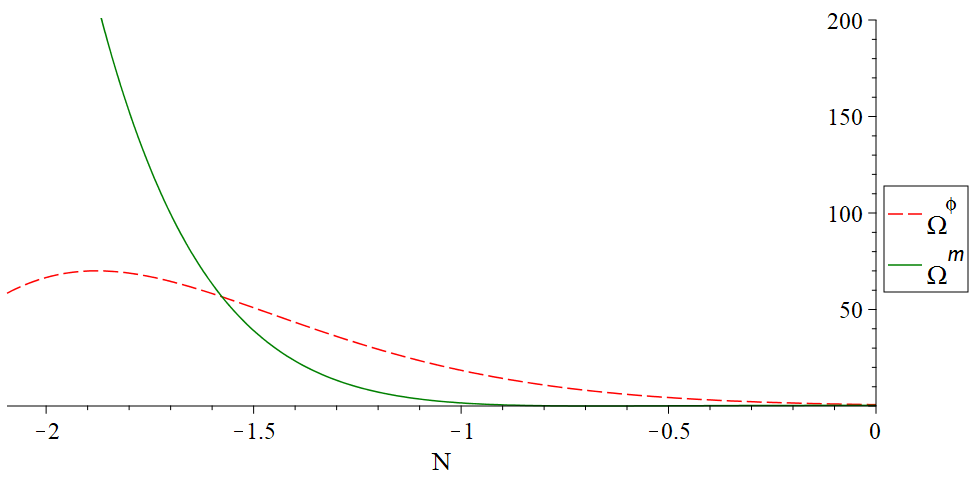
Figure 4: For solutions (58) and (59) with $\beta=1$, the figure schematically (i.e., scale-free) shows the parameters ${\Omega^{\left(m\right)}}$ and ${\Omega^{\left(\phi\right)}}$ versus $N$ as solid and dashed lines, respectively. Besides, the present values of the parameters, i.e. $\Omega^{(m)}_{0}\simeq{0.3}$ and ${\Omega^{(\phi)}_{0}}\simeq{0.7}$, have been used as the initial conditions, and ${a({t_{0}})}=1$.

This figure also indicates that at the beginning of this phase the matter density dominates, and then at the end of its dominance era, the chameleon scalar field density is dominant.

4.3 Case ${\dot{\phi}^{2}}/2=V\left(\phi\right)/2$

In this case, the chameleon potential must again be positive, and hence relations (39) and (40) will hold. Although, one gets ${w^{\left(\phi\right)}}=-1/3$, that is why we have highlighted this case, which also brings almost different results. Accordingly, Eqs. (45) and (46) read

$$2y^{\prime}+3y\simeq\sqrt{2}\,\beta x,$$ (60)

$${}\quad 2x^{\prime}+2x\simeq-\sqrt{2}\,\beta y.$$ (61)

The solutions to these equations with $\beta=3.7\times{10^{2}}$ are

$$y\left(N\right)\!=\frac{{{e^{-\frac{5}{4}N}}}}{{1480}}\!\left[{\left({7{C_{10}}\sqrt{44702}-\!{C_{9}}\sqrt{2}}\right)\sin\!\left({\frac{{7\sqrt{22351}}}{4}N}\right)\!-\!\left({7{C_{9}}\sqrt{44702}-\!{C_{10}}\sqrt{2}}\right)\cos\!\left({\frac{{7\sqrt{22351}}}{4}N}\right)}\right]$$ (62)

and

$$x\left(N\right)={e^{-\frac{5}{4}N}}\left[{{C_{9}}\sin\left({\frac{{7\sqrt{22351}}}{4}N}\right)+{C_{10}}\cos\left({\frac{{7\sqrt{22351}}}{4}N}\right)}\right],$$ (63)

where $C_{9}$ and $C_{10}=x(0)$ are constants of integrations. This time, using solutions (62) and (63), we have plotted ${\Omega^{\left(m\right)}}$ and ${\Omega^{\left(\phi\right)}}$ in Figure 5.

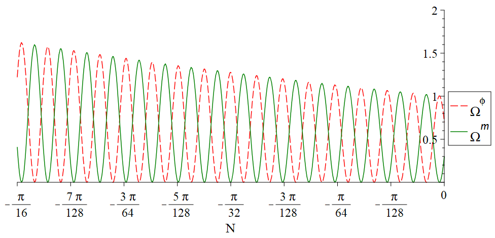
Figure 5: For solutions (62) and (63) with $\beta=3.7\times{10^{2}}$, the figure schematically (i.e., scale-free) shows the parameters ${\Omega^{\left(m\right)}}$ and ${\Omega^{\left(\phi\right)}}$ versus $N$ as solid and dashed lines, respectively. Besides, the present values of the parameters, i.e. $\Omega^{(m)}_{0}\simeq{0.3}$ and ${\Omega^{(\phi)}_{0}}\simeq{0.7}$, have been used as the initial conditions, and ${a({t_{0}})}=1$.

This figure indicates that the behavior of the matter density and the chameleon scalar field density are both also damped oscillations and their values decrease over time.

On the other hand, by considering the non-minimal coupling parameter as $\beta=1$, Eqs. (60) and (61) lead to solutions

$$y\left(N\right)=-\frac{{{e^{-\frac{5}{4}N}}}}{4}\left[{\left({{C_{11}}\sqrt{2}+{C_{12}}\sqrt{14}}\right)\sin\left({\frac{{\sqrt{7}}}{4}N}\right)+\left({{C_{12}}\sqrt{2}-{C_{11}}\sqrt{14}}\right)\cos\left({\frac{{\sqrt{7}}}{4}N}\right)}\right]$$ (64)

and

$$x\left(N\right)={e^{-\frac{5}{4}N}}\left[{{C_{11}}\sin\left({\frac{{\sqrt{7}}}{4}N}\right)+{C_{12}}\cos\left({\frac{{\sqrt{7}}}{4}N}\right)}\right],$$ (65)

where $C_{11}$ and $C_{12}=x(0)$ are constants of integrations. Again using solutions (64) and (65), we have plotted ${\Omega^{\left(m\right)}}$ and ${\Omega^{\left(\phi\right)}}$ in Figure 6.

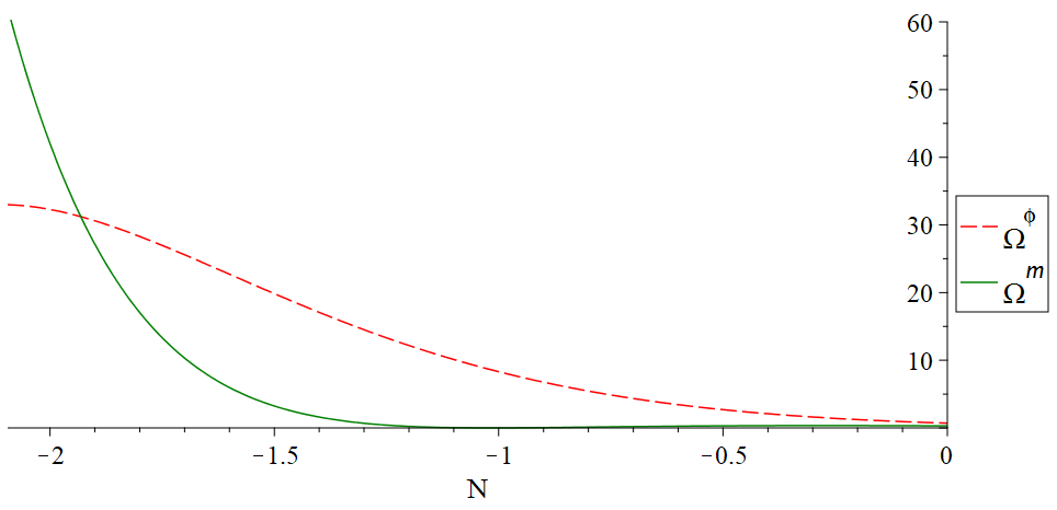
Figure 6: For solutions (64) and (65) with $\beta=1$, the figure schematically (i.e., scale-free) shows the parameters ${\Omega^{\left(m\right)}}$ and ${\Omega^{\left(\phi\right)}}$ versus $N$ as solid and dashed lines, respectively. Besides, the present values of the parameters, i.e. $\Omega^{(m)}_{0}\simeq{0.3}$ and ${\Omega^{(\phi)}_{0}}\simeq{0.7}$, have been used as the initial conditions, and ${a({t_{0}})}=1$.

This figure also shows that at the beginning of this phase, the matter density dominates as assumed, but at the end of its dominance era, the chameleon scalar field density is dominant.

4.4 Case ${\dot{\phi}^{2}}/2\ll V\left(\phi\right)$

Once again, in this case, the chameleon potential must be positive, and accordingly relations (39) and (40) will hold. Moreover, we obviously have ${w^{\left(\phi\right)}}\simeq-1$, hence Eqs. (45) and (46) read

$$2y^{\prime}+3y\simeq 0,$$ (66)

$$2x^{\prime}\simeq 0.$$ (67)

These equations do not depend on the $\beta$ parameter, and we have the solutions

$$y\left(N\right)={y\left(0\right)}{e^{-\frac{3}{2}N}}$$ (68)

and

$$x\left(N\right)={x\left(0\right)},$$ (69)

where $y\left(0\right)=\sqrt{\Omega_{0}^{\left(m\right)}}$ and $x\left(0\right)=\sqrt{\Omega_{0}^{\left(\phi\right)}}$ are the initial conditions at the present-time. Once again, using solutions (68) and (69), we have plotted ${\Omega^{\left(m\right)}}$ and ${\Omega^{\left(\phi\right)}}$ in Figure 7.

Figure 7: For solutions (68) and (69), the figure schematically (i.e., scale-free) shows the parameters ${\Omega^{\left(m\right)}}$ and ${\Omega^{\left(\phi\right)}}$ versus $N$ as solid and dashed lines, respectively. Besides, the present values of the parameters, i.e. $\Omega^{(m)}_{0}\simeq{0.3}$ and ${\Omega^{(\phi)}_{0}}\simeq{0.7}$, have been used as the initial conditions, and ${a({t_{0}})}=1$.

This figure also indicates that at the beginning of this phase, the matter density dominates as assumed, but at the end of its dominance era, the constant density of the chameleon scalar field is dominant.

5 Late-Time Accelerated-Phase

In this section, we investigate the evaluation of the late-time accelerated-phase of the universe via the chameleon scalar field. In this regard, in this accelerated-phase of the universe, by reducing the dust matter density over time, we can assume ${\rho^{\left(\phi\right)}}\gg{\rho^{\left(m\right)}}$. Hence, the equation of state parameter (36) reduces to

$${w^{\left({\rm tot}\right)}}\simeq\frac{{{p^{\left(\phi\right)}}}}{{{\rho^{\left(\phi\right)}}}}={w^{\left(\phi\right)}},$$ (70)

which gives the deceleration parameter (37) as $q\simeq\left({1+3{w^{\left(\phi\right)}}}\right)/2$. Then, in order to achieve $q\leq 0$ in this phase of the universe, one must use ${w^{\left(\phi\right)}}\leq-1/3$, which leads to the constraint ${\dot{\phi}^{2}}\leq V\left(\phi\right)$ with positive potentials in the chameleon model.

On the other hand, in the accelerated-phase of the universe, Eq. (21) yields

$${H^{2}}\simeq H_{0}^{2}{\Omega^{(\phi)}}.$$ (71)

Substituting Eq. (71) into Eqs. (34) and (35) gives

$${{\Omega^{\prime}}^{(m)}}+3{\Omega^{(m)}}\simeq\beta{\Omega^{(m)}}\sqrt{3\left({1+{w^{(\phi)}}}\right)}$$ (72)

and

$${{\Omega^{\prime}}^{(\phi)}}+3{\Omega^{(\phi)}}\left({1+{w^{(\phi)}}}\right)\simeq-\beta{\Omega^{(m)}}\sqrt{3\left({1+{w^{(\phi)}}}\right)}.$$ (73)

Once again, in the following subsections, we probe these solutions for various cases of the relation between the kinetic and potential energies of the scalar field that satisfy the ${\dot{\phi}^{2}}/2\leq V\left(\phi\right)/2$ constraint with positive potentials in the chameleon model. Meanwhile, while using the common power-law chameleon potential (3), we take a brief look at the chameleon scalar field profile in this phase.

5.1 Case ${\dot{\phi}^{2}}/2=V\left(\phi\right)/2$

In this case, we have ${w^{\left(\phi\right)}}=-1/3$, and in turn $q=0$, which is the transition point between the decelerated-epoch and the accelerated-phase in the evaluation of the universe. Hence, Eqs. (72) and (73) with $\beta=3.7\times{10^{2}}$ read

$$\frac{{{{\Omega^{\prime}}^{\left(m\right)}}}}{{{\Omega^{\left(m\right)}}}}\simeq 3.7\times{10^{2}}\sqrt{2}-3$$ (74)

and

$$\frac{{{{\Omega^{\prime}}^{\left(\phi\right)}}}}{{{\Omega^{\left(\phi\right)}}}}\simeq-3.7\times{10^{2}}\sqrt{2}\left({\frac{{{\Omega^{\left(m\right)}}}}{{{\Omega^{\left(\phi\right)}}}}}\right)-2.$$ (75)

The solutions to these equations are

$${{\Omega^{(m)}}}(N)={\Omega^{(m)}_{0}}{e^{\left({3.7\times{10^{2}}\sqrt{2}}-3\right)N}}$$ (76)

and

$${\Omega^{\left(\phi\right)}}(N)=\left\{{\Omega_{0}^{\left(\phi\right)}+\frac{{3.7\times{{10}^{2}}\sqrt{2}\,\Omega_{0}^{\left(m\right)}}}{{273799}}\left({1+3.7\times{{10}^{2}}\sqrt{2}}\right)\left[{1-{e^{\left({3.7\times{{10}^{2}}\sqrt{2}-1}\right)N}}}\right]}\right\}{e^{-2N}}.$$ (77)

We have plotted ${\Omega^{\left(m\right)}}$ and ${\Omega^{\left(\phi\right)}}$ in Figure 8.

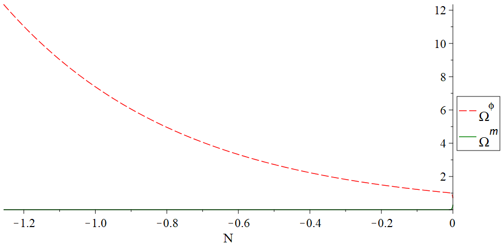
Figure 8: For solutions (76) and (77) with $\beta=3.7\times{10^{2}}$, the figure schematically (i.e., scale-free) shows the parameters ${\Omega^{\left(m\right)}}$ and ${\Omega^{\left(\phi\right)}}$ versus $N$ as solid and dashed lines, respectively. Besides, the present values of the parameters, i.e. $\Omega^{(m)}_{0}\simeq{0.3}$ and ${\Omega^{(\phi)}_{0}}\simeq{0.7}$, have been used as the initial conditions, and ${a({t_{0}})}=1$.

This figure shows that, in this phase of the universe, although the matter density increases slightly, its amount is very negligible all along the path, and the chameleon scalar field density, while decreasing, is dominant at all times.

On the other hand, for $\beta=1$, Eq. (72) gives

$$\frac{{{{\Omega^{\prime}}^{\left(m\right)}}}}{{{\Omega^{\left(m\right)}}}}\simeq\sqrt{2}-3$$ (78)

and, while using the assumption ${\Omega^{\left(m\right)}}\ll{\Omega^{\left(\phi\right)}}$ in the late-time accelerated-phase of the universe, Eq. (73) yields

$$\frac{{{{\Omega^{\prime}}^{\left(\phi\right)}}}}{{{\Omega^{\left(\phi\right)}}}}+2\simeq 0.$$ (79)

The solutions to Eqs. (78) and (79) are

$${{\Omega^{(m)}}}(N)={\Omega^{(m)}_{0}}{e^{\left({\sqrt{2}}-3\right)N}}$$ (80)

and

$${\Omega^{(\phi)}}(N)=\Omega_{0}^{\left(\phi\right)}{e^{-2N}}.$$ (81)

We have plotted ${\Omega^{\left(m\right)}}$ and ${\Omega^{\left(\phi\right)}}$ in Figure 9.

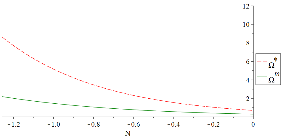
Figure 9: For solutions (80) and (81) with $\beta=1$, the figure schematically (i.e., scale-free) shows the parameters ${\Omega^{\left(m\right)}}$ and ${\Omega^{\left(\phi\right)}}$ versus $N$ as solid and dashed lines, respectively. Besides, the present values of the parameters, i.e. $\Omega^{(m)}_{0}\simeq{0.3}$ and ${\Omega^{(\phi)}_{0}}\simeq{0.7}$, have been used as the initial conditions, and ${a({t_{0}})}=1$.

This figure indicates that the non-relativistic matter density and the chameleon scalar field density both decrease with increasing the scale factor. Although the decrease in the matter density during this epoch of the evolution of the universe is less than that of the chameleon, the chameleon scalar field density dominates at all times.

Continuing the analysis, let us take a brief look at the chameleon scalar field profile while using the common power-law chameleon potential (3). In the case of this subsection, such a potential leads to

$$\dot{\phi}=\pm\sqrt{\frac{{{M^{4+n}}}}{{{\phi^{n}}}}}.$$ (82)

Therefore, the chameleon scalar field is

$${\phi^{\frac{n}{2}+1}}(t)=\pm\left({\frac{n}{2}+1}\right)\sqrt{{M^{4+n}}}\,t+{A(t=0)},$$ (83)

where ${A(t=0)}$ is an integration constant. Furthermore, the constraint $V\left(\phi\right)>0$ indicates that, for the case $\phi>0$, the parameter $n$ can be both odd and even, but for case $\phi<0$, the parameter $n$ can only be even.

5.2 Case ${\dot{\phi}^{2}}/2\ll V\left(\phi\right)$

In this case, we have ${w^{\left(\phi\right)}}\simeq-1$, and in turn $q<0$, hence Eqs. (72) and (73) read

$${\Omega^{\prime\left(m\right)}}+3{\Omega^{\left(m\right)}}\simeq 0$$ (84)

and

$${\Omega^{\prime\left(\phi\right)}}\simeq 0.$$ (85)

These equations do not depend on the $\beta$ parameter, and we have the solutions

$${{\Omega^{(m)}}}(N)={\Omega^{(m)}_{0}}{e^{-3N}}$$ (86)

and

$${\Omega^{(\phi)}}(N)=\Omega_{0}^{\left(\phi\right)}.$$ (87)

We have plotted solutions (86) and (87) in Figure 10.

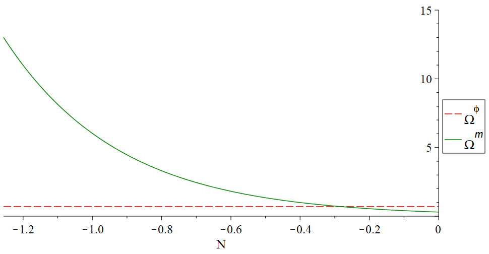
Figure 10: For solutions (86) and (87), the figure schematically (i.e., scale-free) shows the parameters ${\Omega^{\left(m\right)}}$ and ${\Omega^{\left(\phi\right)}}$ versus $N$ as solid and dashed lines, respectively. Besides, the present values of the parameters, i.e. $\Omega^{(m)}_{0}\simeq{0.3}$ and ${\Omega^{(\phi)}_{0}}\simeq{0.7}$, have been used as the initial conditions, and ${a({t_{0}})}=1$.

This figure illustrates that first the matter density dominates, then with the increase of the scale factor, the chameleon scalar field density, while always remaining constant, dominates the late-time accelerated-phase of the universe.

Also, in the case of subsection $5.2$, the common power-law chameleon potential (3) leads to

$$\dot{\phi}\ll\pm\sqrt{\frac{{{2M^{4+n}}}}{{{\phi^{n}}}}}.$$ (88)

Hence, the chameleon scalar field is

$${\phi^{\frac{n}{2}+1}}(t)\ll\pm\left({\frac{n}{2}+1}\right)\sqrt{{2M^{4+n}}}\,t+{B(t=0)},$$ (89)

where ${B(t=0)}$ is an integration constant.

Now, to make our investigations more instructive, let us compare our results with the corresponding one in the $\Lambda CDM$ model. For the $\Lambda CDM$ model, we have

$$S=\int{{d^{4}}x\sqrt{-g}}\left[{\frac{{M_{\rm Pl}^{2}}}{2}\left({R-2\Lambda}\right)+{L^{\left(m\right)}}\left({{\psi^{\left(m\right)}},{g_{\mu\nu}}}\right)}\right],$$ (90)

with the field equations

$${G_{\mu\nu}}=\frac{1}{{M_{\rm Pl}^{2}}}\left({T_{\mu\nu}^{\left(\Lambda\right)}+T_{\mu\nu}^{\left(m\right)}}\right),$$ (91)

where the energy-momentum tensor of the cosmological constant is defined as

$$T_{\mu\nu}^{\left(\Lambda\right)}\equiv-M_{\rm Pl}^{2}\Lambda{g_{\mu\nu}}.$$ (92)

This tensor describes a vacuum state with a constant energy density ${\rho^{\left(\Lambda\right)}}$ and a constant isotropic pressure density ${p^{\left(\Lambda\right)}}$ as

$${\rho^{\left(\Lambda\right)}}=M_{\rm Pl}^{2}\Lambda=-{p^{\left(\Lambda\right)}}.$$ (93)

Assuming the FLRW metric (16) with the matter density as a dust matter perfect fluid, one obtains the Friedmann equations for the $\Lambda CDM$ model as

$${H^{2}}=\frac{\Lambda}{3}+\frac{{{\rho^{\left(m\right)}}}}{{3M_{\rm Pl}^{2}}},$$ (94)

$$\frac{{\ddot{a}}}{a}=\frac{\Lambda}{3}-\frac{{{\rho^{\left(m\right)}}}}{{6M_{\rm Pl}^{2}}}.$$ (95)

Furthermore, the energy-momentum conservation in this model leads to

$${{\dot{\rho}}^{\left(m\right)}}+3H\rho^{\left(m\right)}=0,$$ (96)

$${{\dot{\rho}}^{\left(\Lambda\right)}}=0.$$ (97)

Using the dimensionless density parameters, these are

$${{\Omega^{\prime}}^{\left(m\right)}}+3{\Omega^{\left(m\right)}}=0,$$ (98)

$${{\Omega^{\prime}}^{\left(\Lambda\right)}}=0$$ (99)

that lead to solution (86) and solution like (87), respectively.

Therefore, in the case ${\dot{\phi}^{2}}/2\ll V\left(\phi\right)$ with positive potentials in the chameleon model, i.e. subsections $4.4$ and $5.2$, the behavior obtained for the presented chameleon model is similar to the $\Lambda CDM$ model.

6 Conclusions

By considering the spatially flat FLRW line element as the background geometry, we have investigated the cosmological solutions of the chameleon model. In this model, the scalar field non-minimally couples with the matter field, and its interaction with the ambient matter goes through a conformal factor that leads to a dependence of the chameleon mass on the matter density. Accordingly, the equations of motion of the chameleon scalar field become highly non-linear, hence rather than solving the resulted equations analytically, we have restricted the solutions to proceed.

After deriving the corresponding Friedmann and Raychaudhuri equations, we have manipulated and scrutinized the related field equations for the dimensionless density parameters of the matter field and the scalar field with respect to the e-folding while treating the matter density as a non-relativistic perfect fluid and all variables simply as a function of the cosmic time. Then, we have focused and investigated the cosmological solutions of the chameleon model in the matter-dominated phase and the late-time accelerated-phase of the universe in the context of various cases of the relation between the kinetic and potential energies of the chameleon scalar field, or indeed, for some specific cases of the scalar field equation of state parameter. Thereupon, we have schematically plotted those density parameters versus the e-folding for two different values on the chameleon non-minimal coupling parameter. Meanwhile, we have shown that the assumption of the matter density much more than the chameleon density corresponds to the matter-dominated phase with a decelerated evolution for positive chameleon potential energies. However conversely, the assumption of the chameleon density much more than the matter density can correspond to an accelerated-phase when the scalar field equation of state parameter is less than or equal to $-1/3$ (in this case, the equality corresponds to the deceleration parameter being zero, i.e. the transition point). This situation leads to the case that the kinetic energy of the chameleon scalar field must be less than or equal to half of its potential energy for positive chameleon potentials.

More clearly, for the described chameleon model in the matter-dominated phase, with the non-minimal coupling parameter $\beta=1$, we have indicated that, when the kinetic energy of the chameleon scalar field is much more than the absolute value of, equal to, and equal to half of its potential energy (which respectively correspond to the scalar field equation of state parameter of approximately $+1$, $0$, and $-1/3$), the matter density dominates at the beginning, but then, at the end of its dominance era, the chameleon scalar field density is dominant. Conversely, if the kinetic energy of the chameleon scalar field is much less than its potential energy for positive chameleon potential energies (i.e., when the scalar field equation of state parameter is approximately $-1$), the final result will still be the same as above, but for any non-minimal coupling parameter. That is, the result of this case does not depend on the non-minimal coupling parameter. Also, in this phase with the strong non-minimal coupling parameter $\beta=3.7\times{10^{2}}$, the behavior of the matter density and the chameleon scalar field density, in the first three cases mentioned above, are both damped oscillations, i.e. the value of both densities decreases with increasing scale factor over time.

Furthermore, in the late-time accelerated-phase, first, the plausible assumption of the chameleon density much more than the matter density leads to the total equation of state parameter being almost identical to the scalar field equation of state parameter, the one described at the end of the second paragraph. Then, in the case that the kinetic energy of the chameleon scalar field is equal to half of its potential energy, with the strong non-minimal coupling parameter $\beta=3.7\times{10^{2}}$, we have indicated that, although the matter density increases slightly, its amount is very negligible all along the path and the chameleon scalar field density, while decreasing, is dominant at all times. In this case with the non-minimal coupling parameter $\beta=1$, the matter density and the chameleon scalar field density both decrease, and although the decrease of the matter density is less than that of the chameleon, the chameleon scalar field density dominates at all times. On the other hand, in the case that the kinetic energy of the chameleon scalar field is much less than its potential energy (i.e., when the scalar field equation of state parameter is approximately $-1$), the behavior of the matter density and the chameleon scalar field density do not depend on the non-minimal coupling parameter. In this case, we have shown that first the matter density dominates, then with the increase of the scale factor, the chameleon scalar field density, while always remaining constant, dominates the late-time phase. Also, we have taken a brief look at the chameleon scalar field profile while using the common power-law chameleon potential.

Finally, in both the matter-dominated phase and the late-time accelerated-phase, we have specified that, when the kinetic energy of the chameleon scalar field is much less than its potential energy (i.e., when the scalar field equation of state parameter is approximately $-1$), the behavior obtained for the presented chameleon model is similar to the $\Lambda CDM$ model. Such compatibility suggests that the chameleon model is phenomenologically viable and can be tested with the observational data.

References

- [1] A.H. Guth, “The inflationary universe: A possible solution to the horizon and flatness problems”, Phys. Rev. D 23, 347 (1981).
- [2] A. Albrecht and P.J. Steinhardt, “Cosmology for grand unified theories with radiatively induced symmetry breaking”, Phys. Rev. Lett. 48, 1220 (1982).
- [3] A.D. Linde, Particle Physics and Inflationary Cosmology, (Harwood, Chur, 1990).
- [4] D.H. Lyth and A. Riotto, “Particle physics models of inflation and the cosmological density perturbation”, Phys. Rep. 314, 1 (1999).
- [5] A.R. Liddle and D. Lyth, Cosmological Inflation and Large Scale Structure, (Cambridge University Press, Cambridge, 2000).
- [6] V. Faraoni, “Generalized slow-roll inflation”, Phys. Lett. A 269, 209 (2000).
- [7] S. Weinberg, Cosmology, (Oxford University Press, Oxford, 2008).
- [8] P.A.R. Ade et al., “Planck 2015 results. XIII. Cosmological parameters”, Astron. Astrophys. 594, A13 (2016).
- [9] S. Nojiri and S.D. Odintsov, “Modified gravity with negative and positive powers of the curvature: Unification of the inflation and of the cosmic acceleration”, Phys. Rev. D 68, 123512 (2003).
- [10] N. Saba and M. Farhoudi, “Chameleon field dynamics during inflation”, Int. J. Mod. Phys. D 27, 1850041 (2018).
- [11] S.M.M. Rasouli, N. Saba, M. Farhoudi, J. Marto and P.V. Moniz, “Inflationary universe in deformed phase space scenario”, Ann. Phys. 393, 288 (2018).
- [12] H. Bernardo, R. Costa, H. Nastase and A. Weltman, “Conformal inflation with chameleon coupling”, J. Cosmol. Astropart. Phys. 1904, 027 (2019).
- [13] S. Bhattacharjee, J.R.L. Santos, P.H.R.S. Moraes and P.K. Sahoo, “Inflation in gravity”, Eur. Phys. J. Plus 135, 576 (2020).
- [14] S.D. Odintsov, V.K. Oikonomou and F.P. Fronimos, “Rectifying Einstein-Gauss-Bonnet inflation in view of GW170817”, Nucl. Phys. B 958, 115135 2020.
- [15] M. Faraji, N. Rashidi and K. Nozari, “Inflation in energy-momentum squared gravity in light of Planck 2018”, Eur. Phys. J. Plus 137, 593 (2022).
- [16] X. Zhang, C.Y. Chen and Y. Reyimuaji, “Modified gravity models for inflation: In conformity with observations”, Phys. Rev. D 105, 043514 (2022).
- [17] M. Shiravand, S. Fakhry and M. Farhoudi, “Cosmological inflation in gravity”, Phys. Dark Univ. 37, 101106 (2022).
- [18] N. Aghanim et al., “Planck 2018 results. VI. Cosmological parameters”, Astron. Astrophys. 641, A6 (2020). Erratum: Astron. Astrophys. 652, C4 (2021).
- [19] A. Riess et al., “Observational evidence from supernovae for an accelerating universe and a cosmological constant”, Astron. J. 116, 1009 (1998).
- [20] S. Perlmutter et al. [The Supernovae Cosmology Project], “Measurements of Omega and Lambda from high-redshift supernovae”, Astrophys. J. 517, 565 (1999).
- [21] A.G. Riess et al., “BV RI light curves for type Ia supernovae”, Astron. J. 117, 707 (1999).
- [22] A.G. Riess et al., “Type Ia supernova discoveries at from the Hubble space telescope: Evidence for past deceleration and constraints on dark energy evolution”, Astrophys. J. 607, 665 (2004).
- [23] N. Benitez et al., “Measuring baryon acoustic oscillations along the line of sight with photometric redshifts: The PAU survey”, Astrophys. J. 691, 241 (2009).
- [24] D. Parkinson et al., “Optimizing baryon acoustic oscillation surveys II: Curvature, redshifts and external data sets”, Mon. Not. Roy. Astron. Soc. 401, 2169 (2010).
- [25] B.P. Abbott et al., “A gravitational-wave measurement of the Hubble constant following the second observing run of Advanced LIGO and Virgo”, Astrophys. J. 909, 218 (2021).
- [26] M. Farhoudi, “On higher order gravities, their analogy to GR, and dimensional dependent version of Duff’s trace anomaly relation”, Gen. Rel. Grav. 38, 1261 (2006).
- [27] M. Farhoudi, “Lovelock tensor as generalized Einstein tensor”, Gen. Rel. Grav. 41, 117 (2009).
- [28] T.P. Sotiriou and V. Faraoni, “ theories of gravity”, Rev. Mod. Phys. 82, 451 (2010).
- [29] S. Capozziello and V. Faraoni, Beyond Einstein Gravity: A Survey of Gravitational Theories for Cosmology and Astrophysics, (Springer, London, 2011).
- [30] T. Harko, F.S.N. Lobo, S. Nojiri and S.D. Odintsov, “ gravity”, Phys. Rev. D 84, 024020 (2011).
- [31] S. Capozziello and M. De Laurentis, “Extended theories of gravity”, Phys. Rep. 509, 167 (2011).
- [32] S.M.M. Rasouli, M. Farhoudi and H.R. Sepangi, “Anisotropic cosmological model in modified Brans-Dicke theory”, Class. Quant. Grav. 28, 155004 (2011).
- [33] T. Clifton, P.G. Ferreira, A. Padilla and C. Skordis, “Modified gravity and cosmology”, Phys. Rep. 513, 1 (2012).
- [34] H. Shabani and M. Farhoudi, “ cosmological models in phase-space”, Phys. Rev. D 88, 044048 (2013).
- [35] Z. Haghani, T. Harko, H.R. Sepangi and S. Shahidi, “Matter may matter”, Int. J. Mod. Phys. D 23, 1442016 (2014).
- [36] S.M.M. Rasouli, M. Farhoudi and P.V. Moniz , “Modified Brans-Dicke theory in arbitrary dimensions”, Class. Quant. Grav. 31, 115002 (2014).
- [37] A. Joyce, B. Jain, J. Khoury and M. Trodden, “Beyond the cosmological standard model”, Phys. Rept. 568, 1 (2015).
- [38] P. Bueno, P.A. Cano, A.Ó. Lasso and P.F. Ramírez, “f(Lovelock) theories of gravity”, J. High Energy Phys. 04, 028 (2016).
- [39] N. Khosravi, “Ensemble average theory of gravity”, Phys. Rev. D 94, 124035 (2016).
- [40] S.D. Odintsov, D. Sáez-Chillón Gómez and G.S. Sharov, “Testing viable extensions of Einstein-Gauss-Bonnet gravity”, Phys. Dark Univ. 37, 101100 (2022).
- [41] L.K. Duchaniya, K. Gandhi and B. Mishra, “Cosmological implication of gravity models through phase space analysis”, arXiv: 2303.09076.
- [42] S.M. Carroll, V. Duvvuri, M. Trodden and M.S. Turner, “Is cosmic speed-up due to new gravitational physics?”, Phys. Rev. D 70, 043528 (2004).
- [43] M.C.B. Abdalla, S. Nojiri and S.D. Odintsov, “Consistent modified gravity: Dark energy, acceleration and the absence of cosmic doomsday”, Class. Quant. Grav. 22, L35 (2005).
- [44] S.M. Carroll et al., “The cosmology of generalized modified gravity models”, Phys. Rev. D 71, 063513 (2005).
- [45] S. Capozziello, V.F. Cardone and A. Troisi, “Dark energy and dark matter as curvature effects”, J. Cosmol. Astropart. Phys. 0608, 001 (2006).
- [46] S. Nojiri and S.D. Odintsov, “Introduction to modified gravity and gravitational alternative for dark energy”, Int. J. Geom. Meth. Mod. Phys. 04, 115 (2007).
- [47] A. Borowiec, W. Godlowski and M. Szydlowski, “Dark matter and dark energy as effects of modified gravity”, Int. J. Geom. Meth. Mod. Phys. 04, 183 (2007).
- [48] K. Atazadeh, M. Farhoudi and H.R. Sepangi, “Accelerating universe in brane gravity”, Phys. Lett. B 660, 275 (2008).
- [49] L. Amendola and S. Tsujikawa, Dark Energy: Theory and Observations, (Cambridge University Press, Cambridge, 2010).
- [50] H. Farajollahi, M. Farhoudi, A. Salehi and H. Shojaie, “Chameleonic generalized Brans-Dicke model and late-time acceleration”, Astrophys. Space Sci. 337, 415 (2012).
- [51] A.F. Bahrehbakhsh, M. Farhoudi and H. Vakili, “Dark energy from fifth dimensional Brans-Dicke theory”, Int. J. Mod. Phys. D 22, 1350070 (2013).
- [52] H. Shabani and M. Farhoudi, “Cosmological and solar system consequences of gravity models”, Phys. Rev. D 90, 044031 (2014).
- [53] K. Koyama, “Cosmological tests of modified gravity”, Rept. Prog. Phys. 79, 046902 (2016).
- [54] A. Joyce, L. Lombriser and F. Schmidt, “Dark energy vs. modified gravity”, Ann. Rev. Nucl. Part. Sci. 66, 95 (2016).
- [55] R. Zaregonbadi and M. Farhoudi, “Cosmic acceleration from matter-curvature coupling”, Gen. Rel. Grav. 48, 142 (2016).
- [56] A.F. Bahrehbakhsh, “Interacting induced dark energy model”, Int. J. Theor. Phys. 57, 2881 (2018).
- [57] R. Zaregonbadi, “Cosmic acceleration via space-time-matter theory”, Mod. Phys. Lett. A 34, 1950296 (2019).
- [58] Y. Xu, G. Li, T. Harko and S.-D. Liang, “ gravity”, Eur. Phys. J. C 79, 708 (2019).
- [59] R. Zaregonbadi, N. Saba and M. Farhoudi, “Cosmic acceleration and geodesic deviation in chameleon scalar field models”, Eur. Phys. J. C 82, 730 (2022).
- [60] F. Bajardi R. D’Agostino, “Late-time constraints on modified Gauss-Bonnet cosmology”, Gen. Rel. Grav. 55, 49 (2023).
- [61] F. Zwicky, “On the masses of nebulae and of clusters of nebulae”, Astrophys. J. 86, 217 (1937).
- [62] P.D. Mannheim, “Are galactic rotation curves really flat?”, Astrophys. J. 479, 659 (1997).
- [63] J.M. Overduin and P.S. Wesson, “Dark matter and background light”, Phys. Rept. 402, 267 (2004).
- [64] J. Binny and S. Tremaine, Galactic Dynamics, (Princeton University Press, Princeton, 2nd Ed. 2008).
- [65] M. Milgrom, “A modification of the Newtonian dynamics as a possible alternative to the hidden mass hypothesis”, Astrophys. J. 270, 365 (1983).
- [66] R.H. Sanders, “Finite length-scale anti-gravity and observations of mass discrepancies in galaxies”, Astron. Astrophys. 154, 135 (1986).
- [67] T. Harko and K.S. Cheng, “Galactic metric, dark radiation, dark pressure, and gravitational lensing in brane world models”, Astrophys. J. 636, 8 (2006).
- [68] S. Capozziello, V.F. Cardone and A. Troisi, “Low surface brightness galaxy rotation curves in the low energy limit of gravity: No need for dark matter?”, Mon. Not. Roy. Astron. Soc. 375, 1423 (2007).
- [69] C.F. Martins and P. Salucci, “Analysis of rotation curves in the framework of gravity”, Mon. Not. Roy. Astron. Soc. 381, 1103 (2007).
- [70] A.S. Sefiedgar, Z. Haghani and H.R. Sepangi, “Brane- gravity and dark matter”, Phys. Rev. D 85, 064012 (2012).
- [71] R. Zaregonbadi, M. Farhoudi and N. Riazi, “Dark matter from gravity”, Phys. Rev. D 94, 084052 (2016).
- [72] M. Ishak, “Testing general relativity in cosmology”, Living Rev. Rel. 22, 1 (2019).
- [73] C.M. Will, “The confrontation between general relativity and experiment”, Living Rev. Rel. 9, 3 (2006).
- [74] P.G. Ferreira, “Cosmological tests of gravity”, Ann. Rev. Astron. Astrophys. 57, 335 (2019).
- [75] S. Weinberg, “The cosmological constant problem”, Rev. Mod. Phys. 61, 1 (1989).
- [76] P.J. Steinhardt, Critical Problems in Physics, (Princeton University, Princeton, NJ, 1997).
- [77] S.M. Carroll, “The cosmological constant”, Living Rev. Rel. 4, 1 (2001).
- [78] V. Sahni, “The cosmological constant problem and quintessence”, Class. Quant. Grav. 19, 3435 (2002).
- [79] S.M. Carroll, “Why is the universe accelerating?”, AIP. Conf. Proc. 743, 16 (2004).
- [80] S. Nobbenhuis, “Categorizing different approaches to the cosmological constant problem”, Found. Phys. 36, 613 (2006).
- [81] H. Padmanabhan and T. Padmanabhan, “CosMIn: The solution to the cosmological constant problem”, Int. J. Mod. Phys. D 22, 1342001 (2013).
- [82] D. Bernard and A. LeClair, “Scrutinizing the cosmological constant problem and a possible resolution”, Phys. Rev. D 87, 063010 (2013).
- [83] P. Bull et al., “Beyond CDM: Problems, solutions, and the road ahead”, Phys. Dark Univ. 12, 56 (2016).
- [84] I. Zlatev, L. Wang and P.J. Steinhardt, “Quintessence, cosmic coincidence and the cosmological constant”, Phys. Rev. Lett. 82, 896 (1999).
- [85] P.J. Steinhardt, L. Wang and I. Zlatev, “Cosmological tracking solutions”, Phys. Rev. D 59, 123504 (1999).
- [86] J.P. Ostriker and P.J. Steinhardt, “The quintessential universe”, Sci. Am. 284, 46 (2001).
- [87] P.J.E. Peebles and B. Ratra, “The cosmological constant and dark energy”, Rev. Mod. Phys. 75, 559 (2003).
- [88] T. Padmanabhan, “Cosmological constant: The weight of the vacuum”, Phys. Rep. 380, 235 (2003).
- [89] Y. Fujii and K. Maeda, The Scalar-Tensor Theory of Gravitation, (Cambridge University Press, Cambridge, 2004).
- [90] D. Polarski, “Dark energy: Current issues”, Ann. Phys. (Berlin) 15, 342 (2006).
- [91] E.J. Copeland, M. Sami and S. Tsujikawa, “Dynamics of dark energy”, Int. J. Mod. Phys. D 15, 1753 (2006).
- [92] R. Durrer and R. Maartens, “Dark energy and dark gravity: Theory overview”, Gen. Rel. Grav. 40, 301 (2008).
- [93] V. Faraoni, “Scalar field mass in generalized gravity”, Class. Quant. Grav. 26, 145014 (2009).
- [94] K. Bamba, S. Capozziello, S. Nojiri and S.D. Odintsov, “Dark energy cosmology: The equivalent description via different theoretical models and cosmography tests”, Astrophys. Space Sci. 342, 155 (2012).
- [95] J. Khoury and A. Weltman, “Chameleon cosmology”, Phys. Rev. D 69, 046024 (2004).
- [96] J. Khoury and A. Weltman, “Chameleon fields: Awaiting surprises for tests of gravity in space”, Phys. Rev. Lett. 93, 171104 (2004).
- [97] S. Gubser and J. Khoury, “Scalar self-interactions loosen constraints from fifth force searches”, Phys. Rev. D 70, 104001 (2004).
- [98] P. Brax, C. Van de Bruck, A.-C. Davis, J. Khoury and A. Weltman, “Detecting dark energy in orbit: The cosmological chameleon”, Phys. Rev. D 70, 123518 (2004).
- [99] N. Banerjee, S. Das and K. Ganguly, “Chameleon field and the late time acceleration of the universe”, Pramana 74, 481 (2010).
- [100] H. Farajollahi, A. Salehi, F. Tayebi and A. Ravanpak, “Stability analysis in tachyonic potential chameleon cosmology”, J. Cosmol. Astropart. Phys. 05, 017 (2011).
- [101] J. Khoury, “Chameleon field theories”, Class. Quant. Grav. 30, 214004 (2013).
- [102] P. Brax, A.-C. Davis and J. Sakstein, “Dynamics of supersymmetric chameleons”, J. Cosmol. Astropart. Phys. 1310, 007 (2013).
- [103] N. Roy and N. Banerjee, “Dynamical systems study of chameleon scalar field”, Ann. Phys. 356, 452 (2015).
- [104] I. Quiros, R. García-Salcedo, T. Gonzalez and F.A. Horta-Rangel, “The chameleon effect in the Jordan frame of the Brans-Dicke theory”, Phys. Rev. D 92, 044055 (2015).
- [105] N. Roy, “Dynamical systems analysis of various dark energy models”, PhD. Thesis, Indian Inst. Sci. Educ. Res. Kolkata, (2015).
- [106] C. Burrage and J. Sakstein, “Tests of chameleon gravity”, Living Rev. Rel. 21, 1 (2018).
- [107] N. Saba and M. Farhoudi, “Noncommutative universe and chameleon field dynamics”, Ann. Phys. 395, 1 (2018).
- [108] A. Singh, A. Pradhan and A. Beesham, “Cosmological aspects of anisotropic chameleonic Brans-Dicke gravity”, New Astron. 100, 101995 (2023).
- [109] Z. Yousaf, M.Z. Bhatti, S. Rehman and K. Bamba, “Dynamics of self-gravitating systems in non-linearly magnetized chameleonic Brans-Dicke gravity”, Gen. Rel. Grav. 55, 31 (2023).
- [110] A. Salehi, “Cosmographic test of chameleon gravity”, Gen. Rel. Grav. 55, 34 (2023).
- [111] Y. Boumechta, B.S. Haridasu, L. Pizzuti, M.A. Butt, C. Baccigalupi and A. Lapi, “Constraining chameleon screening using galaxy cluster dynamics”, Phys. Rev. D 108, 044007 (2023).
- [112] A. Paliathanasis, “Dynamical analysis in chameleon dark energy”, Fortsch. Phys. 71, 2300088 (2023).
- [113] A. Paliathanasis, “Reconstruction of universe from Noether symmetries in chameleon gravity”, Phys. Dark Univ. 42, 101275 (2023).
- [114] E.G. Adelberger, B.R. Heckel and A.E. Nelson, “Tests of the gravitational inverse square law, Ann. Rev. Nucl. Part. Sci. 53, 77-121 (2003).
- [115] T. Wagner, S. Schlamminger, J. Gundlach and E. Adelberger, “Torsion-balance tests of the weak equivalence principle”, Class. Quant. Grav. 29, 184002 (2012).
- [116] C. Briddon, C. Burrage, A. Moss and A. Tamosiunas, “SELCIE: A tool for investigating the chameleon field of arbitrary sources”, J. Cosmol. Astropart. Phys. 12, 043 (2021).
- [117] J. Wainwright and G.F.R. Ellis [Editors], Dynamical Systems in Cosmology,, (Cambridge University Press, Cambridge, 1997).
- [118] A.A. Coley, Dynamical Systems with Cosmology, (Kluwer Academic Publishers, Netherlands, 2003).
- [119] C. Burrage and J. Sakstein, “A compendium of chameleon constraints”, J. Cosmol. Astropart. Phys. 11, 045 (2016).
- [120] J. Khoury, “Theories of dark energy with screening mechanisms”, arXiv: 1011.5909.
- [121] M. Roshan and F. Shojai, “Tracking cosmology” Phys. Rev. D 79, 103510 (2009).
- [122] P.G. Ferreira and M. Joyce, “Structure formation with a self-tuning scalar field”, Phys. Rev. Lett. 79, 4740 (1997).
- [123] M. Jaffe et al., “Testing sub-gravitational forces on atoms from a miniature in-vacuum source mass”, Nature 13, 938 (2017).