Decomposed Prompt Tuning via Low-Rank Reparameterization
Abstract
While prompt tuning approaches have achieved competitive performance with high efficiency, we observe that they invariably employ the same initialization process, wherein the soft prompt is either randomly initialized or derived from an existing embedding vocabulary. In contrast to these conventional methods, this study aims to investigate an alternative way to derive soft prompt. Our empirical studies show that the soft prompt typically exhibits a low “intrinsic rank” characteristic. With such observations, we propose decomposed prompt tuning, a novel approach that utilizes low-rank matrices to initialize the soft prompt. Through the low-rank reparameterization, our method significantly reduces the number of trainable parameters while maintaining effectiveness. Experimental results on the SuperGLUE benchmark in both high-resource and low-resource scenarios demonstrate the effectiveness of the proposed method.111Our code is available at https://github.com/XYaoooo/DPT.
1 Introduction
Pre-trained language models Peters et al. (2018); Radford et al. (2019); Devlin et al. (2019); Liu et al. (2020); Raffel et al. (2020) have achieved remarkable performance on various natural language understanding and generation tasks. The pretrain-then-finetune paradigm has been adopted as a common approach to deal with downstream tasks. However, such a paradigm is often considered inefficient, especially in the era of large language models (LLMs), as it requires tuning a large number of model parameters and saving a separate model for each task.
Recently, parameter-efficient fine-tuning (PEFT) approaches Houlsby et al. (2019); mahabadi et al. (2021); Liu et al. (2022b, a); Vu et al. (2022); Asai et al. (2022); Wang et al. (2022, 2023) have been proposed to address this challenge. The main idea of these methods is to fine-tune only a subset of the model’s parameters or additionally introduced parameters while freezing the majority of parameters of a pre-trained model. These approaches require saving only the trainable parameters for different tasks, striking a balance between performance and efficiency.
The success of PEFT methods is also aligned with the previous findings that pre-trained models possess a low “intrinsic rank” Li et al. (2018); Aghajanyan et al. (2020). Aghajanyan et al. (2020) empirically showed that employing a low-dimensional reparameterization is equally effective as full-model fine-tuning. Hu et al. (2022) further demonstrated that weight updates during model training also exhibit a low “intrinsic rank”. By only tuning the proposed low-rank adaptation module, their approach achieves high efficiency while maintaining competitive performance.
Another line of research work focuses on P*-tuning Li and Liang (2021); Liu et al. (2021); Qin and Eisner (2021); Lester et al. (2021). Specifically, Li and Liang (2021) proposed prefix tuning by prepending a sequence of virtual tokens to each transformer layer, and it updates the representations of these virtual tokens while keeping the pre-trained model frozen. Prompt tuning Lester et al. (2021) further simplified prefix tuning by updating only a sequence of continuous prompt tokens in the embedding layer.
Owing to its simplicity, subsequent studies (Ma et al., 2022; Razdaibiedina et al., 2023) continuously improve the vanilla prompt tuning approach. Despite the substantial achievements of these prompt tuning methods, we observe that they invariably employ the same initialization process, wherein the soft prompt is either randomly initialized or derived from the existing embedding vocabulary. Different from the previous approaches, this paper aims to explore an alternative approach to deriving soft prompt.
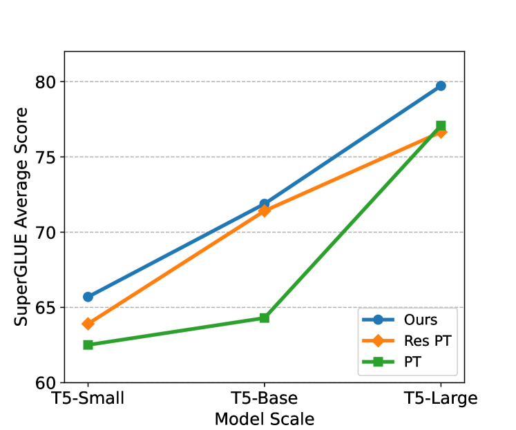
Our motivation stems from the observations that weight updates in the transformer layer during training have a low “intrinsic rank”, as highlighted by Hu et al. (2022). This leads us to inquire whether soft prompt also have a similar low “intrinsic rank” pattern. To this end, we conduct studies examining the “intrinsic rank” of soft prompt, and we include the details of the analysis in Section 2. Based on the studies, we find that the soft prompt indeed tends to exhibit a low “intrinsic rank” behavior. Armed with this insight, we propose decomposed prompt tuning (DPT), a novel approach that employs low-rank matrices to initialize the soft prompt. Specifically, we decompose the original soft prompt into the product of two compact matrices, and we include the detailed description in Section 3. With this low-rank reparameterization, DPT significantly reduces the number of trainable parameters while achieving strong performance. A comparison with previous approaches, depicted in Figure 1, verifies the efficacy of our method.
Our contribution can be summarized as follows:
-
•
We present an empirical study to show that the soft prompt exhibits a low “intrinsic rank” characteristic.
-
•
Motivated by such findings, we propose our method to initialize the soft prompt with low-rank matrices. Experimental results on the SuperGLUE benchmark in both high-resource and low-resource scenarios demonstrate the effectiveness of our proposed approach.
-
•
Compared with the vanilla prompt tuning approach, our method requires significantly fewer trainable parameters while achieving strong performance (i.e., 11.2K vs. 102K with T5-Large).
2 Emergence of “Intrinsic Rank”
To investigate the rank of soft prompt, we design an analysis based on the vanilla prompt tuning approach on the sub-tasks within the SuperGLUE benchmark. Specifically, we re-design the soft prompt, which facilitates a probe into its rank.
2.1 Prompt Tuning
We employ the vanilla prompt tuning Lester et al. (2021) approach to conduct our analysis, as illustrated on the left side of Figure 2. By considering the classification task as a conditional generation task, prompt tuning models the probability as:
| (1) |
where the input is the concatenation of the prepended prompt of length and the original input of length . After the embedding layer, the representations for the prompt and the original input are and , respectively, and is the embedding dimension of the pre-trained model. denotes a sequence of output tokens, which also serves as the class label for the input222 can be a single token or a sequence of tokens.. indicates the frozen parameters of the pre-trained model, while represents the trainable parameter corresponding to the prompt .

2.2 Low-Rank Behavior of Soft Prompt
As highlighted earlier, the soft prompt comprises the only tunable parameters during training. Typically, such a weight matrix in a neural network has a full rank both before and after model training. Therefore, to investigate whether the prompt matrix has a low “intrinsic rank”, we need to reparameterize the soft prompt.
Consider an example matrix , the singular value decomposition of the matrix is in the form of , where , , and is a diagonal matrix. Note that the diagonal entries of represent the singular values of , and the number of non-zero singular values is equal to the rank of . With the above decomposition, we can first reparameterize the soft prompt as:
| (2) |
Here, the matrices and are randomly initialized and set as trainable parameters in this analysis. is initialized with positive values along the diagonal, while the off-diagonal elements are set as 0. We further impose constraints on such that only the diagonal entries are trainable while the remaining are frozen. Intuitively, if the soft prompt has a low “intrinsic rank”, then some of the diagonal entries of will converge to 0 during training. We provide an explanation of why we can use the rank of as an approximation for the rank of in Appendix A.1.
However, due to the dense nature of the neural network, the diagonal entries of can hardly be updated to exact 0. To resolve this challenge, we apply a rectified linear unit (ReLU) to the diagonal matrix :
| (3) |
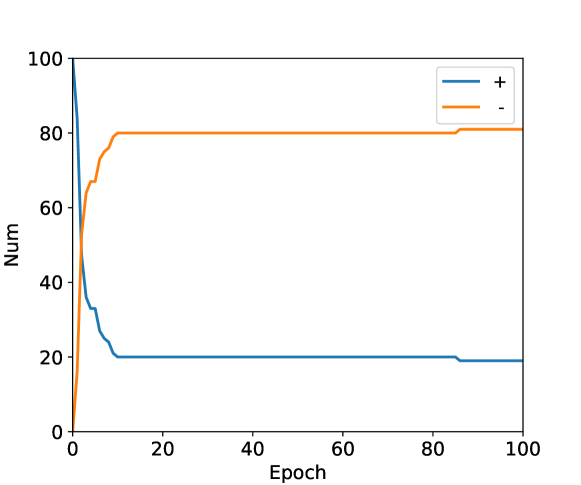
Through such a reparameterization of the soft prompt , we can count the number of positive entries in the rectified diagonal matrix post-training to approximately investigate the rank of the matrix . We can infer that if the soft prompt has a low “intrinsic rank”, more diagonal entries of will be updated to negative values.
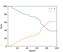
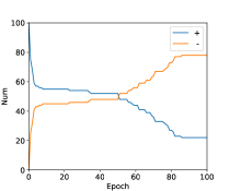
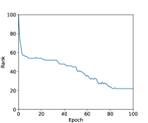
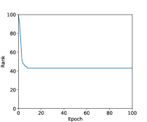
We conduct our empirical experiments with the T5-base model on the CB dataset De Marneffe et al. (2019) of SuperGLUE benchmark, and Figure 3 shows the results. We observe that the number of positive diagonal entries decreases while the number of negative diagonal entries increases as training progresses. We interpret these observations as indicative that the soft prompt has a low “intrinsic rank”. Note that the soft prompt length is set as the commonly used value of 100 in this analysis, this accounts for the initial count of 100 positive diagonal entries. We also observe similar behavior on other datasets with models of different sizes, with additional details provided in Appendix A.2.
3 Method
Motivated by the observation of the soft prompt’s low “intrinsic rank” behavior, as discussed in the previous section, we propose a parameterization of the soft prompt that explicitly constrains it to be of low rank. In this section, we provide the details of our approach, as illustrated on the right side of Figure 2.
3.1 Decomposition of Soft Prompt
As described in Section 2.1, the input of the vanilla prompt tuning approach is the concatenation of the prompt and the input text . The overall input to the pre-trained model is then as follows:
| (4) |
where there are soft prompt tokens and text tokens. The focus of our approach is a more efficient representation of the soft prompt , which usually has dimension .
Instead of using a random initialization for the soft prompt, we decompose it into the product of two matrices:
| (5) |
where and , as illustrated on the right side of Figure 2. One of the main advantages of this representation is that it offers us the ability to modulate the rank of the soft prompt by controlling the size of the intermediary dimension , which we term as the “bottleneck”. Specifically, by setting to a relatively small value, the resulting soft prompt inherently possesses a low rank. Moreover, this decomposition approach affords a reduction in the number of trainable parameters by compressing the bottleneck. Specifically, there are trainable parameters in the vanilla prompt tuning approach. With our proposed DPT approach, the number of trainable parameters is . When setting , the total number of trainable parameters can be significantly reduced. Note that is usually set to 100 and is 1024 for T5-Large Raffel et al. (2020), and we set as 10 in our main experiments. A more detailed analysis of bottleneck can be found in Section 6.1.
3.2 Training and Inference
We adopt similar training procedures as discussed in Section 2.1. Our training objective is as follows:
| (6) |
where indicates the prompt with a length tokens, denotes the frozen parameters of the pre-trained model, and is the trainable parameter associated with the prompt . In our approach, the representation of the soft prompt , is derived as the product of two matrices (Eq. 5), and , which are both initialized randomly and serve as the tunable parameters of our model. corresponds to the parameters contained in matrices and . After the training is completed, we can store the product of and for inference.
4 Experimental Setup
4.1 Datasets
To assess the effectiveness of our proposed DPT method, we conduct experiments on eight datasets from the SuperGLUE benchmark Wang et al. (2019) under both high-resource and low-resource conditions. We follow previous work Lester et al. (2021); Vu et al. (2022) to report the performance of our model on the validation sets due to the restricted access to the test sets of SuperGLUE. We provide detailed descriptions, evaluation metrics, and statistics of the SuperGLUE benchmark in Appendix A.3.
| Model | # Trainable | WSC | WiC | BoolQ | CB | COPA | MultiRC | ReCoRD | RTE | |
|---|---|---|---|---|---|---|---|---|---|---|
| Params. | Acc. | Acc. | Acc. | Acc. | Acc. | F1 | F1 | Acc. | Avg. | |
| T5-Small | ||||||||||
| Fine-Tuning | 60M | 67.94 | 68.18 | 77.06 | 89.28 | 59.00 | 66.98 | 55.64 | 72.56 | 69.58 |
| Prompt Tuning Lester et al. (2021) | 51K | 63.14 | 59.29 | 66.78 | 74.99 | 58.33 | 64.89 | 52.75 | 59.92 | 62.51 |
| Residual PT Razdaibiedina et al. (2023) | 462K | 63.14 | 60.96 | 73.35 | 72.02 | 56.66 | 65.12 | 53.08 | 67.02 | 63.91 |
| Ours | 6K | 63.78 | 64.31 | 71.74 | 79.16 | 58.00 | 64.89 | 53.27 | 70.51 | 65.70 |
| T5-Base | ||||||||||
| Fine-Tuning∗ | 220M | 81.70 | 69.30 | 82.30 | 91.70 | 60.00 | 76.90 | 80.90 | 84.50 | 78.41 |
| Prompt Tuning Lester et al. (2021) | 77K | 64.74 | 59.97 | 62.18 | 70.23 | 56.33 | 72.69 | 71.84 | 56.43 | 64.30 |
| Residual PT Razdaibiedina et al. (2023) | 693K | 67.94 | 63.31 | 80.00 | 77.37 | 56.66 | 72.11 | 72.21 | 81.70 | 71.41 |
| Ours | 9K | 67.30 | 68.49 | 78.64 | 78.56 | 56.66 | 71.22 | 72.53 | 81.94 | 71.88 |
| T5-Large | ||||||||||
| Fine-Tuning∗ | 770M | 88.50 | 73.50 | 88.30 | 94.30 | 87.00 | 85.40 | 89.20 | 90.60 | 87.10 |
| Prompt Tuning Lester et al. (2021) | 102K | 76.52 | 70.00 | 84.09 | 74.40 | 62.00 | 76.18 | 84.51 | 88.95 | 77.08 |
| Residual PT Razdaibiedina et al. (2023) | 925K | 70.50 | 72.25 | 85.04 | 73.21 | 62.66 | 76.46 | 84.36 | 88.92 | 76.67 |
| Ours | 11K | 79.16 | 71.99 | 84.76 | 88.09 | 62.33 | 76.72 | 84.46 | 90.25 | 79.72 |
4.2 Settings
We use the encoder-decoder T5 model Raffel et al. (2020) as the backbone for our experiments. We employ three variants of the T5 model: T5-Small, T5-Base, and T5-Large, which comprise 60M, 220M, and 770M parameters respectively. We implement our approach with the HuggingFace Transformers library Wolf et al. (2020). Each dataset within the SuperGLUE benchmark is converted into a text-to-text format for compatibility with the T5 model. The model is trained for 100 epochs with an initial learning rate of 0.3, and AdamW Loshchilov and Hutter (2019) is employed as the optimizer. The length of the soft prompt is fixed at 100. The embedding dimension is configured as per the model variant, being set to 512, 768, and 1024 for T5-Small, T5-Base, and T5-Large respectively. Importantly, we set the bottleneck size to 10. This bottleneck plays an instrumental role in inducing low-rank constraints on the embedded soft prompt matrix . We initialize the matrices and of our prompt parameters with Gaussian distribution.
4.3 Baselines
To maintain consistency in evaluation metrics and preprocessing procedures across all datasets, we reproduce most of the scores to ensure a fair comparison. More details about implementation can be found in Appendix A.4.
Fine-tuning
We compare DPT with the conventional fine-tuning approach of the T5 modelRaffel et al. (2020), where separate copies of the model must be tuned and stored for different datasets. Though fine-tuning is not a parameter-efficient approach, it is usually treated as an upper bound of performance.
Prompt Tuning
Prompt tuning (PT) Lester et al. (2021) prepends a soft prompt to the input embedding. It adapts to downstream tasks by exclusively updating the parameters of the soft prompt, keeping the language model frozen.
Residual Prompt Tuning
Residual prompt tuning (Residual PT) Razdaibiedina et al. (2023) is a recently proposed variant of PT. It enhances the original prompt embeddings through an additional layer of shallow network instead of passing them directly into the frozen transformer layer. A residual connection is also employed to boost the performance and convergence rate.
Our proposed model is not directly comparable with the multi-stage XPrompt Ma et al. (2022), which iteratively updates the soft prompt embedding. Adapter-based methods Houlsby et al. (2019); Rücklé et al. (2021); Guo et al. (2021) are also not included for comparison in this paper as they require efforts to modify the transformer layers. Furthermore, they often include a considerably larger number of parameters than prompt tuning approaches as mentioned in Razdaibiedina et al. (2023) 333More detailed comparisons can be found in Section 7..
5 Results
5.1 Main Results
Table 1 presents a comparison of our DPT with the vanilla prompt tuning Lester et al. (2021) and residual prompt tuning Razdaibiedina et al. (2023) across 8 datasets from the SuperGLUE benchmark. Besides the model performance, we also include the comparison of the total number of trainable parameters. Remarkably, our model consistently outperforms the aforementioned approaches across T5 models of different sizes in terms of the average scores over the 8 datasets. Specifically, our model outperforms the vanilla prompt tuning by 3.19, 7.58, and 2.64 points in terms of the average score (Avg.) with T5-Small, T5-Base, and T5-Large models, respectively. In most cases, our model surpasses the vanilla prompt tuning approach by a large margin. Moreover, DPT is highly efficient in terms of parameter usage, requiring approximately one-ninth of the number of trainable parameters compared to vanilla prompt tuning (i.e., 11.2K vs. 102K for T5-Large). When compared with the recently proposed residual prompt tuning, our model also shows better or comparable performance. Crucially, DPT achieves this while requiring significantly fewer trainable parameters. Specifically, residual prompt tuning consumes nearly 84 times more parameters than our method (i.e., 11.2K vs. 925K for T5-Large). Note that we set the length of the soft prompt for residual prompt tuning to 100 which empirically yields better performance 444There are 100-token and 10-token residual prompt tuning variants in the original paper Razdaibiedina et al. (2023).. We also provide the experimental results of residual prompt tuning when setting the length of the soft prompt to 10 in Appendix A.6. The experimental results demonstrate the effectiveness of our proposed low-rank soft prompt in both performance and parameter efficiency.
5.2 Few-shot Performance
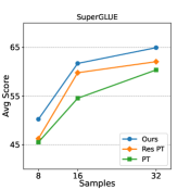
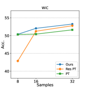
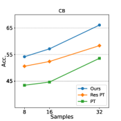
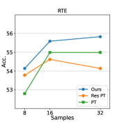
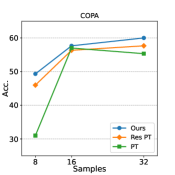
We further evaluate our method in a few-shot setting on all datasets in the SuperGLUE benchmark. Specifically, we sample total of 8, 16, and 32 training instances without balancing the label distribution to mimic a realistic scenario. To ensure a fair comparison, the sampled data for our method, vanilla prompt tuning, and residual prompt tuning are kept identical for each run. We employ the T5-Large model as the backbone for this evaluation as it achieves the strongest performance in the vanilla prompt tuning. The results presented are averaged across three separate runs with different random seeds. We compare our approach against the previous methods in terms of the average score over all datasets in the SuperGLUE benchmark, and the results are shown in Figure 4(a). We observe that our method consistently outperforms both vanilla prompt tuning and residual prompt tuning in our experiments. Additionally, We also include experimental results on specific datasets from SuperGLUE in Figure 4(b), 4(c), 4(d), and 4(e). These results further demonstrate the effectiveness of our method over the baselines in the few-shot setting.
6 Analysis
6.1 Sensitivity of Bottleneck Size
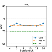
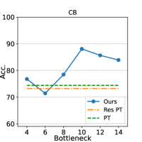
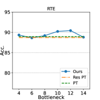
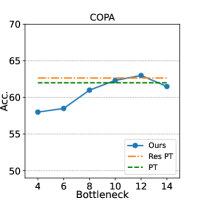
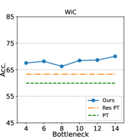
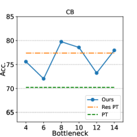
As mentioned in Section 3.1, the rank of our soft prompt can be adjusted through the bottleneck . In this section, we investigate how the size of the bottleneck impacts the performance of DPT. We conduct experiments using T5-Large on the WiC, CB, RTE, and COPA datasets, with bottleneck . The results are shown in Figure 5. We can see that though our approach experiences performance fluctuations with different sizes of the bottleneck , DPT outperforms the vanilla prompt tuning and residual prompt tuning in quite a few cases. Intuitively, the size of the bottleneck plays a critical role in the expressiveness of our model. We observe a performance drop when the size of the bottleneck is getting smaller. We find similar behavior when T5-Base is used, and the results can be found in Appendix A.7.
6.2 Effect of Prompt Length
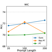
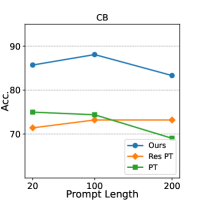
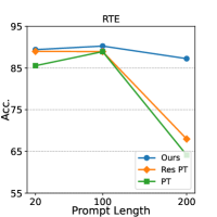
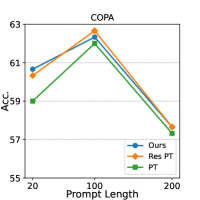
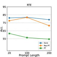
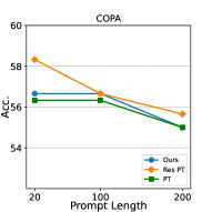
To investigate the effect of prompt length on the performance of our proposed method, we conduct an analysis on four of the SuperGLUE tasks555These four datasets are randomly selected for analysis., and the results are shown in Figure 6. The prompt length is set as 20, 100, and 200. We use the T5-large model as the backbone, while the bottleneck variable is held constant at 10. As mentioned in Section 3, the number of trainable parameters in the vanilla PT is , whereas for our DPT method, it is . The benefit of our approach in terms of parameter-efficiency is more pronounced as the prompt length increases666When and are fixed, the ratio decreases as the prompt length increases. This implies that our method exhibits higher parameter efficiency with longer prompt lengths.. We observe that our DPT consistently outperforms the vanilla prompt tuning approach across various prompt lengths. Moreover, DPT is generally found to be comparable or superior to residual prompt tuning. Corroborating the observations made by Lester et al. (2021), a long soft prompt does not necessarily improve the model performance. While a prompt length of 100 has been empirically validated as an effective hyperparameter in previous work Lester et al. (2021); Razdaibiedina et al. (2023), our analysis reveals that the performance gains can still be achieved with a prompt length of 200, as illustrated in Figure 6(a). Furthermore, our DPT is less sensitive to the change of prompt length on CB and RTE, as shown in Figure 6(b) and Figure 6(c). We observe similar behavior when switching to T5-Base as the backbone, and details are included in Appendix A.8.
6.3 Constrained Bottleneck under Short Prompt
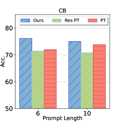
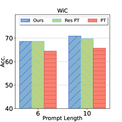
A critical aspect we sought to address with DPT is the potential to sustain both parameter efficiency and competitive performance, even with a short prompt. When the prompt length is reduced to values such as 6 or 10, DPT may not exhibit parameter efficiency if the bottleneck remains to be 10. To explore the possibility of achieving parameter efficiency under such conditions, we compress the bottleneck to an extremely low value of 2. The experiments conducted on the CB and WiC tasks using the T5-Large model are illustrated in Figure 7. Notably, even with the bottleneck compressed to such a small value, our method is still able to surpass baselines. This demonstrates that our method is able to effectively generalize to extremely short prompts. Similar results can be observed on T5-base in Appendix A.9.
6.4 Bottleneck vs. Number of Trainable Parameters
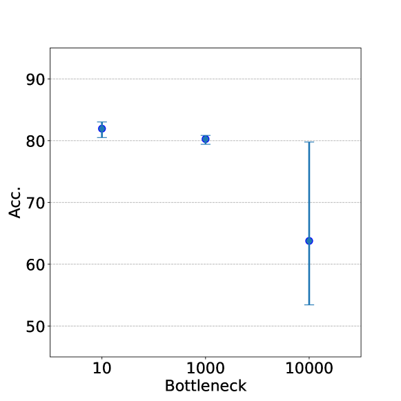
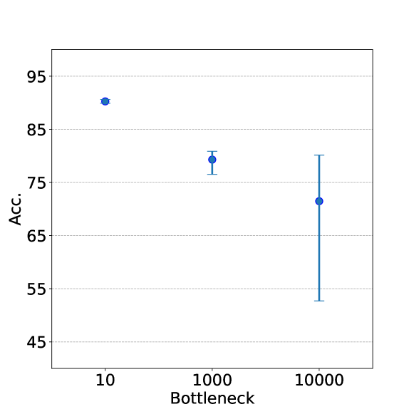
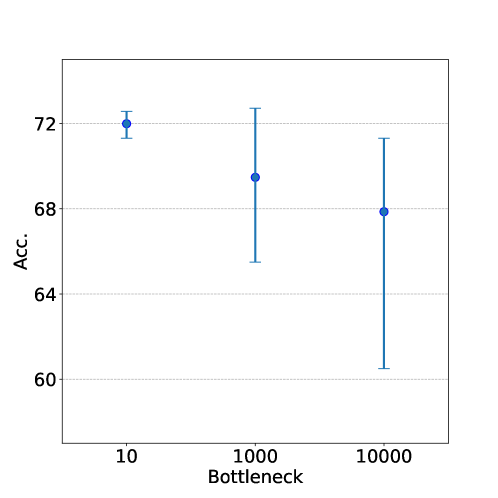
To further study the effect of bottleneck size without considering parameter efficiency, we conduct experiments with the bottleneck of varying magnitudes, specifically , while maintaining a fixed prompt length of 100 tokens. The experimental results are on the RTE dataset with the T5-Large model, and we record the average, minimal, and maximum scores across three runs. Figure 8 shows the comparison, and it is noteworthy that the number of trainable parameters involved are 11.2K, 1.1M, and 11.2M respectively for the varying bottleneck sizes. When configuring the bottleneck to a large value, the soft prompt ceases to be a low-rank matrix and the number of trainable parameters is more than that of a vanilla prompt tuning approach. More importantly, we observe that increasing the number of trainable parameters does not necessarily lead to an enhancement in performance. Furthermore, overparameterization could deteriorate the stability of the performance. We observe similar results with T5-Base model, and the details are included in Appendix A.10.
7 Related Work
Parameter-efficient fine-tuning (PEFT) methods He et al. (2022a); Ben Zaken et al. (2022); He et al. (2022b); Mao et al. (2022); He et al. (2022c) have emerged as a popular approach to fine-tune language model which can largely reduce the number of trainable parameters while maintaining competitive performance. There are two primary paradigms for current PEFT methods: adapter-based and prompt-based approaches.
Adapter-based Method
The concept of the adapter was originally proposed by Houlsby et al. (2019). They inserted a down projection layer followed by an up projection layer in each sub-module of the transformer sequentially. When adapting a model to downstream tasks, only the parameters of the adapter were updated Pfeiffer et al. (2021); Sung et al. (2022); Chen et al. (2023); Zeng et al. (2023). To enhance this, Karimi Mahabadi et al. (2021) incorporated hypernetworks, which generate weights for the main network, thus enabling shared information capture across tasks. Following that, Hu et al. (2022) proposed LoRA to approximate the update of the neural weight. LoRA was based on the assumption that the change in weights during model adaptation has a low “intrinsic rank”. Different from the adapter, LoRA did not introduce additional latency. Apart from being a PEFT method, the adapter has also been employed in broader applications in natural language processing Pfeiffer et al. (2021).
Our work diverges from LoRA Hu et al. (2022) and the broader adapter framework. Rather than learning updates to the parameters, our approach directly learns the parameters, under the hypothesis that the soft prompt inherently exhibits a low “intrinsic rank”. Furthermore, LoRA focuses on Query-specific and Value-specific parameters within the transformer architecture, whereas our approach adheres to the prompt tuning paradigm, where trainable parameters are exclusively inserted in the embedding layer. Despite these fundamental differences, it is noteworthy that both our approach and LoRA share an underlying principle of leveraging low-rank structures.
Prompt-based Method
Prompt-based methods can be categorized into hard prompt and soft prompt approaches. Hard prompts involve adding a fixed sequence of discrete tokens for the model to condition on for generation Jiang et al. (2020); Shin et al. (2020); Zhao et al. (2021); Liu et al. (2023). However, they are sensitive to slight changes and require complex designs, like verbalizer selection. To address this, trainable soft prompt methods were introduced. Li and Liang (2021) introduced prefix tuning, which adds virtual tokens in each layer of the encoder stack. As a simplification of prefix tuning, Prompt Tuning Lester et al. (2021) only adds a soft prompt to the embedding layer. Further advancements include incorporating soft prompts across all transformer layers to enhance performance Liu et al. (2022b). Additionally, transfer learning-based methods Wang et al. (2023); Vu et al. (2022) have been explored for better prompt initialization through pre-training. For instance, Wang et al. (2023) performed pre-training to learn a soft prompt on a collection of source tasks and subsequently employed the acquired prompt embeddings as initialization for target tasks. Transfer learning-based techniques offer the potential for better initialization and more effective prompt tuning. In contrast to prior work, this paper focuses on developing a more efficient parameterization of the soft prompt.
8 Conclusion
In this work, we uncover the low “intrinsic rank” behavior inherent in the soft prompt through empirical examination. Motivated by these findings, we introduce Decomposed Prompt Tuning (DPT), a novel approach that reparameterizes the soft prompt using two compact matrices. By adjusting the bottleneck, DPT enables the effective manipulation of the soft prompt matrix, ensuring it maintains a low rank. Notably, DPT attains strong performance across the SuperGLUE benchmark in high-resource and low-resource scenarios while substantially reducing the number of trainable parameters.
Limitations
Despite our proposed approach being simple but effective, our method still possesses a few limitations. We mainly evaluate our model on the natural understanding tasks, i.e., SuperGLUE. We do not evaluate our proposed method on the natural language generation tasks, and we leave it for future work. Furthermore, our method also inherits a few drawbacks from the vanilla prompt tuning, such as slow convergence. These limitations serve as future directions for further improvement. Another limitation is that we only evaluate our method with the encoder-decoder backbone models. We leave the explorations with encoder-only models and other large-scale pre-trained models for future work.
Acknowledgements
We would like to thank the anonymous reviewers for their constructive comments.
References
- Aghajanyan et al. (2020) Armen Aghajanyan, Luke Zettlemoyer, and Sonal Gupta. 2020. Intrinsic dimensionality explains the effectiveness of language model fine-tuning. In Proceedings of ACL.
- Aribandi et al. (2022) Vamsi Aribandi, Yi Tay, Tal Schuster, Jinfeng Rao, Huaixiu Steven Zheng, Sanket Vaibhav Mehta, Honglei Zhuang, Vinh Q. Tran, Dara Bahri, Jianmo Ni, Jai Gupta, Kai Hui, Sebastian Ruder, and Donald Metzler. 2022. Ext5: Towards extreme multi-task scaling for transfer learning. In Proceedings of ICLR.
- Asai et al. (2022) Akari Asai, Mohammadreza Salehi, Matthew Peters, and Hannaneh Hajishirzi. 2022. ATTEMPT: Parameter-efficient multi-task tuning via attentional mixtures of soft prompts. In Proceedings of EMNLP.
- Ba et al. (2016) Jimmy Lei Ba, Jamie Ryan Kiros, and Geoffrey E. Hinton. 2016. Layer normalization. In Proceedings of NeurIPS.
- Ben Zaken et al. (2022) Elad Ben Zaken, Yoav Goldberg, and Shauli Ravfogel. 2022. BitFit: Simple parameter-efficient fine-tuning for transformer-based masked language-models. In Proceedings of ACL.
- Chen et al. (2023) Tianrun Chen, Lanyun Zhu, Chaotao Deng, Runlong Cao, Yan Wang, Shangzhan Zhang, Zejian Li, Lingyun Sun, Ying Zang, and Papa Mao. 2023. Sam-adapter: Adapting segment anything in underperformed scenes. In Proceedings of ICCV.
- De Marneffe et al. (2019) Marie-Catherine De Marneffe, Mandy Simons, and Judith Tonhauser. 2019. The commitmentbank: Investigating projection in naturally occurring discourse. In proceedings of Sinn und Bedeutung.
- Devlin et al. (2019) Jacob Devlin, Ming-Wei Chang, Kenton Lee, and Kristina Toutanova. 2019. BERT: Pre-training of deep bidirectional transformers for language understanding. In Proceedings of NAACL.
- Guo et al. (2021) Demi Guo, Alexander Rush, and Yoon Kim. 2021. Parameter-efficient transfer learning with diff pruning. In Proceedings of ACL.
- He et al. (2022a) Junxian He, Chunting Zhou, Xuezhe Ma, Taylor Berg-Kirkpatrick, and Graham Neubig. 2022a. Towards a unified view of parameter-efficient transfer learning. In Proceedings of ICLR.
- He et al. (2022b) Shwai He, Liang Ding, Daize Dong, Jeremy Zhang, and Dacheng Tao. 2022b. SparseAdapter: An easy approach for improving the parameter-efficiency of adapters. In Proceedings of EMNLP.
- He et al. (2022c) Yun He, Steven Zheng, Yi Tay, Jai Gupta, Yu Du, Vamsi Aribandi, Zhe Zhao, Yaguang Li, Zhao Chen, Donald Metzler, Heng-Tze Cheng, and Ed H. Chi. 2022c. HyperPrompt: Prompt-based task-conditioning of transformers. In Proceedings of ICLR.
- Houlsby et al. (2019) Neil Houlsby, Andrei Giurgiu, Stanislaw Jastrzebski, Bruna Morrone, Quentin De Laroussilhe, Andrea Gesmundo, Mona Attariyan, and Sylvain Gelly. 2019. Parameter-efficient transfer learning for NLP. In Proceedings of ICML.
- Hu et al. (2022) Edward J Hu, yelong shen, Phillip Wallis, Zeyuan Allen-Zhu, Yuanzhi Li, Shean Wang, Lu Wang, and Weizhu Chen. 2022. LoRA: Low-rank adaptation of large language models. In Proceedings of ICLR.
- Jiang et al. (2020) Zhengbao Jiang, Frank F. Xu, Jun Araki, and Graham Neubig. 2020. How Can We Know What Language Models Know? Transactions of the Association for Computational Linguistics.
- Karimi Mahabadi et al. (2021) Rabeeh Karimi Mahabadi, Sebastian Ruder, Mostafa Dehghani, and James Henderson. 2021. Parameter-efficient multi-task fine-tuning for transformers via shared hypernetworks. In Proceedings of ACL.
- Lester et al. (2021) Brian Lester, Rami Al-Rfou, and Noah Constant. 2021. The power of scale for parameter-efficient prompt tuning. In Proceedings of EMNLP.
- Li et al. (2018) Chunyuan Li, Heerad Farkhoor, Rosanne Liu, and Jason Yosinski. 2018. Measuring the intrinsic dimension of objective landscapes. In Proceedings of ICLR.
- Li and Liang (2021) Xiang Lisa Li and Percy Liang. 2021. Prefix-tuning: Optimizing continuous prompts for generation. In Proceedings of ACL.
- Liu et al. (2022a) Haokun Liu, Derek Tam, Mohammed Muqeeth, Jay Mohta, Tenghao Huang, Mohit Bansal, and Colin A Raffel. 2022a. Few-shot parameter-efficient fine-tuning is better and cheaper than in-context learning. In Proceedings of NeurIPS.
- Liu et al. (2023) Pengfei Liu, Weizhe Yuan, Jinlan Fu, Zhengbao Jiang, Hiroaki Hayashi, and Graham Neubig. 2023. Pre-train, prompt, and predict: A systematic survey of prompting methods in natural language processing. ACM Comput. Surv.
- Liu et al. (2022b) Xiao Liu, Kaixuan Ji, Yicheng Fu, Weng Tam, Zhengxiao Du, Zhilin Yang, and Jie Tang. 2022b. P-tuning: Prompt tuning can be comparable to fine-tuning across scales and tasks. In Proceedings of ACL.
- Liu et al. (2021) Xiao Liu, Yanan Zheng, Zhengxiao Du, Ming Ding, Yujie Qian, Zhilin Yang, and Jie Tang. 2021. Gpt understands, too. arXiv:2103.10385.
- Liu et al. (2020) Yinhan Liu, Myle Ott, Naman Goyal, Jingfei Du, Mandar Joshi, Danqi Chen, Omer Levy, Mike Lewis, Luke Zettlemoyer, and Veselin Stoyanov. 2020. Ro{bert}a: A robustly optimized {bert} pretraining approach.
- Loshchilov and Hutter (2019) Ilya Loshchilov and Frank Hutter. 2019. Decoupled weight decay regularization. In Proceedings of ICLR.
- Ma et al. (2022) Fang Ma, Chen Zhang, Lei Ren, Jingang Wang, Qifan Wang, Wei Wu, Xiaojun Quan, and Dawei Song. 2022. XPrompt: Exploring the extreme of prompt tuning. In Proceedings of EMNLP.
- mahabadi et al. (2021) Rabeeh Karimi mahabadi, James Henderson, and Sebastian Ruder. 2021. Compacter: Efficient low-rank hypercomplex adapter layers. In Proceedings of ICLR.
- Mao et al. (2022) Yuning Mao, Lambert Mathias, Rui Hou, Amjad Almahairi, Hao Ma, Jiawei Han, Scott Yih, and Madian Khabsa. 2022. UniPELT: A unified framework for parameter-efficient language model tuning. In Proceedings of ACL.
- Peters et al. (2018) Matthew E. Peters, Mark Neumann, Mohit Iyyer, Matt Gardner, Christopher Clark, Kenton Lee, and Luke Zettlemoyer. 2018. Deep contextualized word representations. In Proceedings of ACL.
- Pfeiffer et al. (2021) Jonas Pfeiffer, Aishwarya Kamath, Andreas Rücklé, Kyunghyun Cho, and Iryna Gurevych. 2021. AdapterFusion: Non-destructive task composition for transfer learning. In Proceedings of EACL.
- Qin and Eisner (2021) Guanghui Qin and Jason Eisner. 2021. Learning how to ask: Querying LMs with mixtures of soft prompts. In Proceedings of NAACL.
- Radford et al. (2019) Alec Radford, Jeffrey Wu, Rewon Child, David Luan, Dario Amodei, Ilya Sutskever, et al. 2019. Language models are unsupervised multitask learners. OpenAI blog.
- Raffel et al. (2020) Colin Raffel, Noam Shazeer, Adam Roberts, Katherine Lee, Sharan Narang, Michael Matena, Yanqi Zhou, Wei Li, and Peter J. Liu. 2020. Exploring the limits of transfer learning with a unified text-to-text transformer. Journal of Machine Learning Research.
- Razdaibiedina et al. (2023) Anastasia Razdaibiedina, Yuning Mao, Rui Hou, Madian Khabsa, Mike Lewis, Jimmy Ba, and Amjad Almahairi. 2023. Residual prompt tuning: Improving prompt tuning with residual reparameterization. In Proceedings of ACL.
- Rücklé et al. (2021) Andreas Rücklé, Gregor Geigle, Max Glockner, Tilman Beck, Jonas Pfeiffer, Nils Reimers, and Iryna Gurevych. 2021. AdapterDrop: On the efficiency of adapters in transformers. In Proceedings of EMNLP.
- Shin et al. (2020) Taylor Shin, Yasaman Razeghi, Robert L. Logan IV, Eric Wallace, and Sameer Singh. 2020. AutoPrompt: Eliciting Knowledge from Language Models with Automatically Generated Prompts. In Proceedings of EMNLP.
- Sung et al. (2022) Yi-Lin Sung, Jaemin Cho, and Mohit Bansal. 2022. Vl-adapter: Parameter-efficient transfer learning for vision-and-language tasks. In Proceedings of CVPR.
- Vu et al. (2022) Tu Vu, Brian Lester, Noah Constant, Rami Al-Rfou’, and Daniel Cer. 2022. SPoT: Better frozen model adaptation through soft prompt transfer. In Proceedings of ACL.
- Wang et al. (2019) Alex Wang, Yada Pruksachatkun, Nikita Nangia, Amanpreet Singh, Julian Michael, Felix Hill, Omer Levy, and Samuel Bowman. 2019. Superglue: A stickier benchmark for general-purpose language understanding systems. In Proceedings of NeurIPS.
- Wang et al. (2022) Yaqing Wang, Sahaj Agarwal, Subhabrata Mukherjee, Xiaodong Liu, Jing Gao, Ahmed Hassan Awadallah, and Jianfeng Gao. 2022. AdaMix: Mixture-of-adaptations for parameter-efficient model tuning. In Proceedings of EMNLP.
- Wang et al. (2023) Zhen Wang, Rameswar Panda, Leonid Karlinsky, Rogerio Feris, Huan Sun, and Yoon Kim. 2023. Multitask prompt tuning enables parameter-efficient transfer learning. In Proceedings of ICLR.
- Wolf et al. (2020) Thomas Wolf, Lysandre Debut, Victor Sanh, Julien Chaumond, Clement Delangue, Anthony Moi, Pierric Cistac, Tim Rault, Remi Louf, Morgan Funtowicz, Joe Davison, Sam Shleifer, Patrick von Platen, Clara Ma, Yacine Jernite, Julien Plu, Canwen Xu, Teven Le Scao, Sylvain Gugger, Mariama Drame, Quentin Lhoest, and Alexander Rush. 2020. Transformers: State-of-the-art natural language processing. In Proceedings of EMNLP.
- Zeng et al. (2023) Guangtao Zeng, Peiyuan Zhang, and Wei Lu. 2023. One network, many masks: Towards more parameter-efficient transfer learning. In Proceedings of ACL.
- Zhao et al. (2021) Zihao Zhao, Eric Wallace, Shi Feng, Dan Klein, and Sameer Singh. 2021. Calibrate before use: Improving few-shot performance of language models. In Proceedings of ICML.
Appendix A Appendix
A.1 Rank Explanation
Theorem A.1.
Let A and B be matrices such that the product AB is well defined. Then
Proof.
Each column of is a combination of the columns of , which implies that . Hence, , or equivalently, Each row of is a combination of the rows of rowspace rowspace , but the dimension of rowspace dimension of column space , so that . ∎
According to theorem A.1, if , it can be easily obtained that:
is an upper bound of , because and are always full rank during training process. Thus, we can use as an approximation for .
A.2 Record of Rank Change
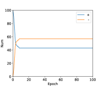
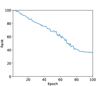
We conduct additional experiments with different models and datasets to probe the rank change of soft prompt. We find consistent observations that the soft prompt tends to exhibit a low “intrinsic rank” behavior. As we can see from Figure 9, the number of positive entries is decreasing while the number of negative entries is increasing. In the second row, we also record the rank change of the soft prompt. Specifically, we calculate the rank of the matrix obtained by multiplying , , and .
A.3 Dataset Details
We record the statistical details of the SuperGLUE benchmark and the metrics we use, and Table 2 shows the statistics. Note that the original CB dataset has 554 training samples, we follow Raffel et al. (2020) to keep only 259 samples with a "True" label. We transform the task to a text-to-text format. Specifically, we highlight the ambiguous pronoun in the input text and ask the model to predict the noun that it refers to Raffel et al. (2020).
| Dataset | Train | Dev | Task | Metric |
| BoolQ | 9,427 | 3,270 | QA | Acc. |
| CB | 250 | 56 | NLI | Acc. |
| COPA | 400 | 100 | QA | Acc. |
| MultiRC | 27,243 | 4,848 | QA | F1 |
| ReCoRD | 100,730 | 10,000 | QA | F1 |
| WiC | 5,428 | 638 | WSD | Acc. |
| WSC | 259 | 104 | Coref. | Acc. |
| RTE | 2,490 | 277 | NLI | Acc. |
A.4 Baseline Implementation Details
The length of the soft prompt is set as 100 for vanilla prompt tuning, which is an optimal setting according to the paper Lester et al. (2021). The soft prompt can be initialized by Gaussian distribution or copying from the vocabulary embedding. Here, we adopt the second initialization strategy because of its superiority.
There are 10-token and 100-token residual prompt tuning variants Razdaibiedina et al. (2023). We implement the 100-token one because it has better performance. We also follow the paper to set the bottleneck as 400, above which leads to no improvement according to the paper. We follow them to adopt ReLU as activation function and perform layer normalization Ba et al. (2016).
| Model | WSC | WiC | BoolQ | CB | COPA | MultiRC | ReCoRD | RTE |
|---|---|---|---|---|---|---|---|---|
| T5-Small | ||||||||
| PT | 1.10 | 2.82 | 1.28 | 3.57 | 1.15 | 0.90 | 0.30 | 3.12 |
| Res PT | 1.10 | 5.7 | 1.64 | 4.12 | 0.57 | 0.51 | 0.22 | 3.68 |
| Ours | 0.55 | 0.65 | 0.85 | 4.12 | 4.35 | 0.90 | 0.15 | 1.98 |
| T5-Base | ||||||||
| PT | 1.10 | 6.30 | 0.01 | 1.02 | 1.15 | 0.24 | 0.09 | 0.20 |
| Res PT | 0.55 | 3.68 | 10.11 | 10.46 | 2.08 | 0.20 | 0.13 | 1.50 |
| Ours | 0.96 | 1.33 | 0.79 | 6.43 | 2.08 | 0.46 | 0.10 | 1.30 |
| T5-Large | ||||||||
| PT | 1.92 | 1.04 | 0.82 | 1.03 | 0.00 | 0.18 | 0.09 | 0.20 |
| Res PT | 3.08 | 0.56 | 0.13 | 1.79 | 1.52 | 0.04 | 0.17 | 0.75 |
| Ours | 1.46 | 0.63 | 0.27 | 2.06 | 2.51 | 0.39 | 0.15 | 0.36 |
| Model | # Trainable | WSC | WiC | BoolQ | CB | COPA | MultiRC | ReCoRD | RTE | |
|---|---|---|---|---|---|---|---|---|---|---|
| Params. | Acc. | Acc. | Acc. | Acc. | Acc. | F1 | F1 | Acc. | Avg. | |
| T5-Small | ||||||||||
| Residual PT | 416K | 64.73 | 58.09 | 69.70 | 73.21 | 58.66 | 63.21 | 52.82 | 62.21 | 62.83 |
| T5-Base | ||||||||||
| Residual PT | 624K | 68.26 | 66.87 | 79.11 | 74.99 | 57.66 | 71.20 | 72.41 | 68.58 | 69.88 |
| T5-Large | ||||||||||
| Residual PT | 832K | 69.86 | 69.74 | 84.18 | 70.82 | 59.33 | 74.77 | 84.31 | 88.20 | 75.15 |
A.5 Standard Deviation of Scores
We report the the standard deviation of three runs for our method, prompt tuning and residual prompt tuning. The results are shown in Table 3.
A.6 Residual PT of 10 tokens
In most parts of this paper, we focus on soft prompt of 100 tokens. Razdaibiedina et al. (2023) present 10-token and 100-token variant of residual prompt tuning in their main results. We reproduce the 100-token residual prompt tuning in the main result section. Here, we also reproduce the 10-token one in Table 4 . The results are consistent with the original paper that the performance of 10-token version is inferior to that of 100-token version.
A.7 Various Bottleneck Size
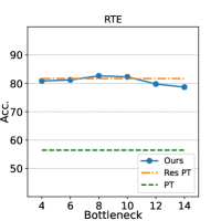
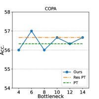
We try different bottleneck and fix prompt length as 100. The result of T5-Base is similar to that of T5-Large. DPT can surpass prompt tuning in most cases, which demonstrates the robustness of DPT. In Figure 10, we show the result on T5-Base.
A.8 Various Prompt Length
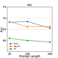
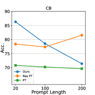
We try prompt length 20, 100 and 200 and fix the bottleneck as 10. The result of T5-Base is similar to that of T5-Large. The performance of DPT is consistently better than PT under various prompt lengths as shown in Figure 11.
A.9 Short Prompt
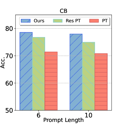
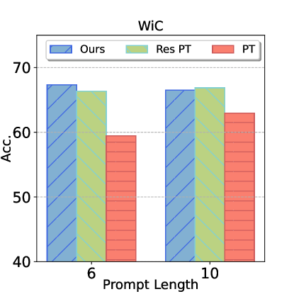
We experiment on WiC dataset and CB dataset to explore that if DPT can work under a very short prompt. We fix the bottleneck as 2, and prompt length can be 6 and 10. We observe that DPT can even work when the soft prompt is extremely short on T5-Base in Figure 12.
A.10 Bottleneck vs. Number of Trainable Parameters
When we enlarge the bottleneck to explore the performance of DPT, we find that an extremely large bottleneck will harm the stability and performance of DPT. The result is consistent when we conduct experiments on both T5-Large and T5-Base. In Figure 13 and 14, we show the results on RTE dataset.
