A Simple Uniformly Optimal Method without Line Search for Convex Optimization

Abstract

Line search (or backtracking) procedures have been widely employed into first-order methods for solving convex optimization problems, especially those with unknown problem parameters (e.g., Lipschitz constant). In this paper, we show that line search is superfluous in attaining the optimal rate of convergence for solving a convex optimization problem whose parameters are not given a priori. In particular, we present a novel accelerated gradient descent type algorithm called auto-conditioned fast gradient method (AC-FGM) that can achieve an optimal $\mathcal{O}(1/k^{2})$ rate of convergence for smooth convex optimization without requiring the estimate of a global Lipschitz constant or the employment of line search procedures. We then extend AC-FGM to solve convex optimization problems with Hölder continuous gradients and show that it automatically achieves the optimal rates of convergence uniformly for all problem classes with the desired accuracy of the solution as the only input. Finally, we report some encouraging numerical results that demonstrate the advantages of AC-FGM over the previously developed parameter-free methods for convex optimization.

1 Introduction

In this paper, we consider the basic convex optimization problem

$$f^{*}:=\min_{x\in X}f(x)$$ (1.1)

where $X\subseteq\mathbb{R}^{n}$ is a closed convex set and $f:X\rightarrow\mathbb{R}$ is a proper convex lower semicontinuous function. We assume that $f$ is represented by a first-order oracle, which, upon request, returns $f(x)$ and $g(x)\in\partial f(x)$. Here, $\partial f(x)$ denotes the subdifferential of $f(\cdot)$ at $x\in X$, and $g(x)$ denotes one of its subgradients. Throughout the paper we assume that the set of optimal solutions $X^{*}$ is nonempty, and let $x^{*}$ denote an arbitrary point in $X^{*}$.

Different problem classes of convex optimization have been studied in the literature. A problem is said to be nonsmooth if its objective function $f$, although not necessarily differentiable, is Lipschtiz continuous, i.e.,

$$|f(x)-f(y)|\leq M\|x-y\|,~{}~{}\forall x,y\in X.$$ (1.2)

It is well-known that the classic subgradient descent method exhibits an $\mathcal{O}(1/\sqrt{k})$ rate of convergence for nonsmooth convex optimization nemirovski1983problem . Here $k$ denotes the number of calls to the first-order oracle. This convergence rate can be significantly improved for smooth problems which have a differentiable objective function $f$ with Lipschtiz continuous gradient $g$ such that

$$\|g(x)-g(y)\|\leq L\|x-y\|,~{}~{}\forall x,y\in X.$$ (1.3)

Specifically, while the gradient descent method exhibits only an $\mathcal{O}(1/k)$ rate of convergence for smooth problems, the celebrated accelerated gradient descent (AGD) method developed by Nesterov nesterov1983method has an $\mathcal{O}(1/k^{2})$ rate of convergence (see also YudinNemirovski77 ; NemirovskiYudin83-smooth ; nemirovski1983problem for Nemirovski and Yudin’s earlier developments on AGD). Between nonsmooth and smooth problems there exists a class of weakly smooth problems with Hölder continuous gradient, i.e.,

$$\|g(x)-g(y)\|\leq L_{\nu}\|x-y\|^{\nu},~{}~{}\text{for some }\nu\in(0,1).$$ (1.4)

Clearly, when $\nu=0$ this condition also indicates (1.2), and when $\nu=1$ it reduces to (1.3). Nemirovski and Nesterov nemirovskii1985optimal showed that the AGD method has an

$$\mathcal{O}\left(\left(\tfrac{L_{\nu}\|x_{0}-x^{*}\|^{1+\nu}}{\epsilon}\right)^{\frac{2}{1+3\nu}}\right)$$

rate of convergence for solving weakly smooth problems. In a more recent work, Lan Lan08-1 further showed that AGD with a properly defined stepsize policy also exhibits an $\mathcal{O}(1/\sqrt{k})$ rate of convergence for nonsmooth (and stochastic) problems. Therefore, AGD is considered to be an optimal method for solving different classes of convex optimization problems, since its rates of convergence match well the lower complexity bounds for smooth, nonsmooth, and weakly smooth problems established by Nemirvoski and Yudin in nemirovski1983problem .

However, in order to achieve these optimal rates of convergence, one needs to first know which problem class $f$ belongs to, and then supply AGD with prior knowledge about $f$, including parameters like $L$, $\nu$, and $L_{\nu}$, as the input of the algorithm. These constants can be unavailable or difficult to compute in many practice scenarios. Additionally, problem classification and parameter estimation over a global scope of $f$ may lead to overly conservative stepsize choices and as a consequence can slow down convergence of the algorithm. To alleviate these concerns, Lan Lan13-1 suggested studying the so-called uniformly optimal methods, signifying that they can achieve the optimal convergence guarantees across all classes of smooth, weakly smooth, and nonsmooth convex optimization problems without requiring much information on problem parameters. Moreover, by noticing that the classic bundle-level method LNN does not require any problem parameters for nonsmooth optimization, Lan Lan13-1 introduced a few novel accelerated bundle-level type methods that are uniformly optimal for convex optimization. These methods can terminate based on the gap between computable upper and lower bounds without using the target accuracy in the updating formula for the iterates. However, these bundle-level type methods require the solution of a more complicated subproblem than AGD in each iteration. In addition, the analysis in Lan13-1 requires the feasible region $X$ to be bounded, which may not hold in some applications. In an effort to address these issues, Nesterov in an important work Nest14 presented a new fast gradient method (FGM) obtained by incorporating a novel line search (or backtracking) procedure armijo1966minimization into the AGD method. He showed that FGM achieves uniformly (or universally) the optimal rate of convergence for solving smooth, weakly smooth, and nonsmooth convex optimization problems with the accuracy of the solution as the only input. While the cost per iteration of FGM might be higher than AGD due to the line search procedure, the total number of calls to the first-order oracle will still be in the same order of magnitude as AGD up to a constant factor. Further developments for adaptive AGD methods with line search can be found in roulet2017sharpness ; liang2023unified ; renegar2022simple ; grimmer2023optimal ; lu2023accelerated , among others.

Due to the wide deployment of first-order methods in data science and machine learning, the past few years have witnessed a growing interest in the development of easily implementable parameter-free first-order methods that have guaranteed fast rates of convergence. One notable line of research is to eliminate the incorporation of line search procedures in first-order methods to further speed up their convergence and reduce the cost per iteration. Specifically, in some interesting works, chaudhuri2009parameter ; streeter2012no ; orabona2016coin ; cutkosky2017online ; cutkosky2018black ; orabona2020tutorial ; mhammedi2020lipschitz studied the problem of parameter-free regret minimization that pertains to nonsmooth convex optimization, carmon2022making ; defazio2023learning ; ivgi2023dog developed adaptive line-search free subgradient type methods for nonsmooth objectives, while levy2017online ; li2019convergence ; malitsky2019adaptive ; malitsky2023adaptive ; khaled2023dowg ; latafat2023adaptive ; orabona2023normalized established the convergence guarantees for this type of method for smooth objectives. However, all the aforementioned methods at most match the convergence rate of non-accelerated (sub)gradient descent in the worst case, thus failing to achieve the optimal rates of convergence for smooth and weakly smooth problems with $\nu\in(0,1]$. It is worth noting that there exist a few accelerated variants of adaptive gradient type methods with $\mathcal{O}(1/k^{2})$ rate for smooth objectives levy2018online ; ene2021adaptive . However, these methods require the stepsize to either depend on the diameter of a bounded feasible region or be fine-tuned according to the unknown initial distance $\|x_{0}-x^{*}\|$. To the best of our knowledge, there does not exist any optimal first-order method that offers simple subproblems, does not assume the feasible region to be bounded, and does not require the line search procedures for solving smooth optimization problems with unknown Lipschitz constant $L$, not to mention the existence of this type of method uniformly optimal for smooth, weakly smooth and nonsmooth convex optimization.

In this paper, we attempt to address the aforementioned open issue in the development of optimal methods for convex optimization. Our major contributions are briefly summarized as follows. Firstly, we introduce a novel first-order algorithm, called Auto-Conditioned Fast Gradient Method (AC-FGM), which can achieve the optimal $\mathcal{O}(1/k^{2})$ convergence rate for smooth convex optimization without knowing any problem parameters or resorting to any line search procedures. The algorithmic framework, being as simple as the AGD method, can completely adapt to the problem structure. The major novelty of AC-FGM lies in the management of two extrapolated sequences of search points, with one serving as the “prox-centers” and the other used for gradient computation, respectively. This design plays an essential role in getting rid of line search required by Nest14 and removing the assumption of a bounded feasible region used in Lan13-1 . Moreover, we propose a novel stepsize policy that is highly adaptive to the local smoothness level, which can lead to more efficient empirical performance compared with other existing adaptive methods. Secondly, we show that AC-FGM can be extended to solve convex problems with Hölder continuous gradients, requiring no prior knowledge of problem parameters except for the desired accuracy of the solution. Our analysis demonstrates that AC-FGM is uniformly optimal for all smooth, weakly smooth, and nonsmooth objectives with $\nu\in[0,1]$. Additionally, we extend AC-FGM to solve composite optimization problems while preserving the same convergence guarantees. Thirdly, we confirm the theoretical advantages of AC-FGM through a series of numerical experiments. Our results show that AC-FGM outperforms the previously developed parameter-free methods, such as the adaptive gradient descent and Nesterov’s FGM, across a wide range of testing problems.

It is worth noting that we focus on convex problems with the function optimality gap as the termination criterion for our algorithms in this paper. We do not consider strongly convex or nonconvex problems. However, Lan, Ouyang and Zhang in a concurrent paper LanOuyangZhang2023 show that by using AC-FGM as a subroutine in their new algorithmic framework, one can achieve tight complexity bounds to minimize (projected) gradients for convex, strongly convex and nonconvex problems in a parameter-free manner. Therefore, the results reported in this work may have an impact in the broader area of parameter-free optimization methods.

The remaining part of the paper is organized as follows. In Section 2, we propose AC-FGM and prove its optimal convergence guarantees for solving smooth convex problems. In Section 3, we extend AC-FGM to solve problems with Hölder continuous gradients and establish its uniform optimality. Section 4 further extends AC-FGM to solve the composite optimization problems. Finally, in Section 5, we provide numerical experiments that demonstrate the empirical advantages of AC-FGM.

1.1 Notation

In this paper, we use the convention that $\tfrac{0}{0}=0$, and $\tfrac{a}{0}=+\infty$ if $a>0$. Unless stated otherwise, we let $\langle\cdot,\cdot\rangle$ denote the Euclidean inner product and $\|\cdot\|$ denote the corresponding Euclidean norm ($\ell_{2}$-norm). Given a vector $x\in\mathbb{R}^{n}$, we denote its $i$-th entry by $x^{(i)}$. Given a matrix $A$, we denote its $(i,j)$-th entry by $A_{i,j}$. We use $\|A\|$ to denote the spectral norm of matrix $A$. We let $\lambda_{\max}(A)$ and $\lambda_{\min}(A)$ denote the largest and smallest eigenvalue of a self-adjoint matrix $A$.

2 AC-FGM for smooth convex problems

In this section, we first consider the case when $f$ is smooth, satisfying condition (1.3) or equivalently,

$$\tfrac{1}{2L}\|g(y)-g(x)\|^{2}\leq f(y)-f(x)-\langle g(x),y-x\rangle\leq\tfrac{L}{2}\|y-x\|^{2},\quad\forall x,y\in X.$$ (2.1)

Our goal is to present a new parameter-free AGD type optimal algorithm that does not require line search for solving this class of problems.

We start to introduce the basic algorithmic framework of the Auto-Conditioned Fast Gradient Method (AC-FGM).

Algorithm 1 Auto-Conditioned Fast Gradient Method (AC-FGM)

Input: initial point $z_{0}=y_{0}=x_{0}$, nonnegative parameters $\beta_{t}\in[0,1)$, $\eta_{t}\in\mathbb{R}_{+}$ and $\tau_{t}\in\mathbb{R}_{+}$.

for $k=1,\cdots,K$ do

     

$$z_{t} =\arg\min_{z\in X}\left\{\eta_{t}\langle g(x_{t-1}),z\rangle+\tfrac{1}{2}\|y_{t-1}-z\|^{2}\right\},$$ (2.2)

$$y_{t} =(1-\beta_{t})y_{t-1}+\beta_{t}z_{t},$$ (2.3)

$$x_{t} =(z_{t}+\tau_{t}x_{t-1})/({1+\tau_{t}}).$$ (2.4)

end for

As shown in Algorithm 1, the basic algorithmic scheme is conceptually simple. It involves three intertwined sequences of search points, $\{x_{t}\}$, $\{y_{t}\}$, and $\{z_{t}\}$, where $\{x_{t}\}$ and $\{y_{t}\}$ are two weighted average sequences of $\{z_{t}\}$. The sequence $\{x_{t}\}$ is used for gradient computation and also represents the output solutions, while $\{y_{t}\}$ is the sequence of “prox-centers” of the prox-mapping problems in (2.2). The search point $z_{t}$ is updated according to (2.2) by minimizing a linear approximation of $f$ at $x_{t-1}$, but not moving too far away from the prox-center $y_{t-1}$ with $\eta_{t}$ as the stepsize.

To illustrate further some basic ideas behind the design of AC-FGM, let us compare it with a few other well-known first-order algorithms in the literature.

• Nesterov’s accelerated gradient method: Nesterov’s accelerated gradient method can be expressed using three sequences of search points (see, e.g., Section 3.3 of LanBook2020 ):

  $$y_{t} =(1-q_{t})x_{t-1}+q_{t}z_{t-1},$$

  $$z_{t} =\arg\min_{z\in X}\left\{\eta_{t}\langle g(y_{t}),z\rangle+\tfrac{1}{2}\|z_{t-1}-z\|^{2}\right\},$$

  $$x_{t} =(1-\alpha_{t})x_{t-1}+\alpha_{t}z_{t}.$$

  Notably, the gradients are computed at $\{y_{t}\}$ rather than the output solutions $\{x_{t}\}$. Additionally, it uses $\{z_{t}\}$ as the prox-centers, while AC-FGM uses the sequence $\{y_{t}\}$, a dynamically weighted average of $\{z_{t}\}$, as the prox-centers.

• Gradient extrapolation method (GEM): GEM lan2018random ; ilandarideva2023accelerated is another method related to AC-FGM, which carries a particular duality relationship with Nesterov’s accelerated gradient method and also achieves the optimal rate of convergence for smooth convex optimization. The algorithm follows the steps

  $$\tilde{g}_{t} =g(x_{t-1})+\alpha_{t}(g(x_{t-1})-g(x_{t-2})),$$

  $$z_{t} =\arg\min_{z\in X}\left\{\eta_{t}\langle\tilde{g}_{t},z\rangle+\tfrac{1}{2}\|z_{t-1}-z\|^{2}\right\},$$

  $$x_{t} =(z_{t}+\tau_{t}x_{t-1})/({1+\tau_{t}}).$$

  Notice that the last step of GEM is the same as AC-FGM, which generates search points for both gradient computation and solution output. The difference between these two methods exists in that GEM utilizes extrapolation in the dual space as in the first step. It is noteworthy that this dual extrapolation idea is also used in the operator extrapolation (OE) method kotsalis2022simple ; kotsalis2022simple1 for solving variational inequalities (VIs).

• Golden ratio method for variational inequalities: The idea of using an extrapolated sequence $\{y_{t}\}$ as the prox-centers was introduced in the Golden ratio method malitsky2020golden ; alacaoglu2023beyond for VIs:

  $$z_{t} =\arg\min_{z\in X}\left\{\eta_{t}\langle F(y_{t-1}),z\rangle+\tfrac{1}{2}\|y_{t-1}-z\|^{2}\right\},$$

  $$y_{t} =(1-\beta_{t})y_{t-1}+\beta_{t}z_{t},$$

  where $F(\cdot)$ is the VI operator. It is shown in malitsky2020golden ; alacaoglu2023beyond that the Golden ratio method is a fully adaptive approach for smooth VIs without requiring the line search procedures. However, one can only achieve an $\mathcal{O}(1/k)$ rate for smooth VIs, which differs from the optimal convergence rate for smooth convex optimization. Therefore, we construct another sequence of search points $\{x_{t}\}$ as in GEM and shift the gradient estimations to accelerate the convergence rate to $\mathcal{O}(1/k^{2})$. In summary, the relationship between AC-FGM and the golden ratio method resembles the relationship between GEM and the OE method in that the former approaches (i.e., AC-FGM and GEM) accelerate the rate of convergence for the latter methods (i.e., Golden ration method and OE) applied to smooth convex optimization.

In the remaining part of this section, we establish the convergence guarantees for AC-FGM and specify the selection of algorithmic parameters $\eta_{t}$, $\beta_{t}$ and $\tau_{t}$. To ensure that AC-FGM operates in a problem-parameter-free manner, we suppose that we do not possess prior knowledge of the smoothness parameter $L$ in conditions (1.3) and (2.1). Instead, we estimate the local smoothness level in each iteration. In the first iteration ($t=1$), we select an initial stepsize $\eta_{1}$ such that $x_{1}\neq x_{0}$ and calculate $L_{1}$ as

$$L_{1}:=\frac{\|g(x_{1})-g(x_{0})\|}{\|x_{1}-x_{0}\|}.$$ (2.5)

For subsequent iterations ($t\geq 2$), we calculate

$$L_{t}:=\begin{cases}~{}0,&\text{if}~{}~{}f(x_{t-1})-f(x_{t})-\langle g(x_{t}),x_{t-1}-x_{t}\rangle=0,\\ \frac{\|g(x_{t})-g(x_{t-1})\|_{*}^{2}}{2[f(x_{t-1})-f(x_{t})-\langle g(x_{t}),x_{t-1}-x_{t}\rangle]},&\text{if}~{}~{}f(x_{t-1})-f(x_{t})-\langle g(x_{t}),x_{t-1}-x_{t}\rangle>0.\end{cases}$$ (2.6)

Notice that this approach allows us to calculate $L_{t}$ whenever a new search point $x_{t}$ is obtained in each iteration. Because the search point $x_{t}$ is calculated using the parameters $\eta_{t}$ and $\tau_{t}$, to obtain the line-search free property, the parameters $\eta_{t}$ and $\tau_{t}$ should be chosen according to the local estimations $L_{1},...,L_{t-1}$ but not $L_{t}$.

The following two results (i.e., Proposition 1 and Theorem 2.1) characterize the convergence behavior and the line-search free property of Algorithm 1. It should be noted that our analysis differs significantly from the existing analyses of the golden ratio method and gradient extrapolation method, and thus appears to be nontrivial. Proposition 1 below provides an important recursive relationship for the iterates of the AC-FGM algorithm.

Proposition 1

Assume the parameters $\{\tau_{t}\}$, $\{\eta_{t}\}$ and $\{\beta_{t}\}$ satisfy

$$\tau_{1} =0,~{}\beta_{1}=0,~{}\beta_{t}=\beta>0,~{}t\geq 2$$ (2.7)

$$\eta_{2} \leq\min\left\{2(1-\beta)\eta_{1},\tfrac{\beta}{2L_{1}}\right\},$$ (2.8)

$$\eta_{t} \leq\min\left\{2(1-\beta)^{2}\eta_{t-1},\tfrac{\beta\tau_{t-1}}{4L_{t-1}},\tfrac{\tau_{t-2}+1}{\tau_{t-1}}\cdot\eta_{t-1}\right\},~{}t\geq 3$$ (2.9)

where $L_{1}$ and $L_{t},~{}t\geq 2$ are defined in (2.5) and (2.6), respectively. We have for any $z\in X$,

$$\textstyle\sum_{t=1}^{k}\eta_{t+1}\left[\tau_{t}f(x_{t})+\langle g(x_{t}),x_{t}-z\rangle-\tau_{t}f(x_{t-1})\right]+\tfrac{\eta_{2}}{2\eta_{1}}\left[\|z_{1}-y_{1}\|^{2}+\|z_{2}-z_{1}\|^{2}\right]$$

$$\leq\tfrac{1}{2\beta}\|y_{1}-z\|^{2}-\tfrac{1}{2\beta}\|y_{k+1}-z\|^{2}+\textstyle\sum_{t=2}^{k+1}\Delta_{t},$$ (2.10)

where

$$\Delta_{t} :=\begin{cases}\eta_{2}\langle g(x_{1})-g(x_{0}),z_{1}-z_{2}\rangle-\tfrac{\beta\|z_{2}-y_{1}\|^{2}}{2},&~{}~{}t=2\\ \eta_{t}\langle g(x_{t-1})-g(x_{t-2}),z_{t-1}-z_{t}\rangle-\tfrac{\eta_{t}\tau_{t-1}\|g(x_{t-1})-g(x_{t-2})\|^{2}}{2L_{t-1}}-\tfrac{\beta\|z_{t}-y_{t-1}\|^{2}}{2},&~{}~{}t\geq 3.\end{cases}$$

Proof

First, by the optimality condition of step (2.2), we have for $t\geq 1$,

$$\langle\eta_{t}g(x_{t-1})+z_{t}-y_{t-1},z-z_{t}\rangle\geq 0,\quad\forall z\in X,$$ (2.11)

and consequently for $t\geq 2$,

$$\langle\eta_{t-1}g(x_{t-2})+z_{t-1}-y_{t-2},z_{t}-z_{t-1}\rangle\geq 0.$$ (2.12)

By (2.3), we have the relationship $z_{t-1}-y_{t-2}=\tfrac{1}{1-\beta_{t-1}}(z_{t-1}-y_{t-1})$, so we can rewrite (2.12) as

$$\langle\eta_{t}g(x_{t-2})+\tfrac{\eta_{t}}{\eta_{t-1}(1-\beta_{t-1})}(z_{t-1}-y_{t-1}),z_{t}-z_{t-1}\rangle\geq 0.$$ (2.13)

Summing up (2.11) and (2.13) and rearranging the terms give us for $t\geq 2$,

$$\eta_{t}\langle g(x_{t-1}),z-z_{t-1}\rangle+\eta_{t}\langle g(x_{t-1})-g(x_{t-2}),z_{t-1}-z_{t}\rangle$$

$$+\langle z_{t}-y_{t-1},z-z_{t}\rangle+\tfrac{\eta_{t}}{\eta_{t-1}(1-\beta_{t-1})}\langle z_{t-1}-y_{t-1},z_{t}-z_{t-1}\rangle\geq 0$$

By utilizing the fact that $2\langle x-y,z-x\rangle=\|y-z\|^{2}-\|x-y\|^{2}-\|x-z\|^{2}$ on the last two terms of the above inequality, we obtain

$$\eta_{t}\langle g(x_{t-1}),z-z_{t-1}\rangle+\eta_{t}\langle g(x_{t-1})-g(x_{t-2}),z_{t-1}-z_{t}\rangle$$

$$+\tfrac{1}{2}\|y_{t-1}-z\|^{2}-\tfrac{1}{2}\|z_{t}-y_{t-1}\|^{2}-\tfrac{1}{2}\|z_{t}-z\|^{2}$$

$$+\tfrac{\eta_{t}}{\eta_{t-1}(1-\beta_{t-1})}\left[\tfrac{1}{2}\|z_{t}-y_{t-1}\|^{2}-\tfrac{1}{2}\|z_{t-1}-y_{t-1}\|^{2}-\tfrac{1}{2}\|z_{t}-z_{t-1}\|^{2}\right]\geq 0,$$ (2.14)

Meanwhile, (2.3) also indicates that

$$\|z_{t}-z\|^{2} =\|\tfrac{1}{\beta_{t}}(y_{t}-z)-\tfrac{1-\beta_{t}}{\beta_{t}}(y_{t-1}-z)\|^{2}$$

$$\overset{(i)}{=}\tfrac{1}{\beta_{t}}\|y_{t}-z\|^{2}-\tfrac{1-\beta_{t}}{\beta_{t}}\|y_{t-1}-z\|^{2}+\tfrac{1}{\beta_{t}}\cdot\tfrac{1-\beta_{t}}{\beta_{t}}\|y_{t}-y_{t-1}\|^{2}$$

$$=\tfrac{1}{\beta_{t}}\|y_{t}-z\|^{2}-\tfrac{1-\beta_{t}}{\beta_{t}}\|y_{t-1}-z\|^{2}+(1-\beta_{t})\|z_{t}-y_{t-1}\|^{2},$$ (2.15)

where step (i) follows from the fact that $\|\alpha a+(1-\alpha)b\|^{2}=\alpha\|a\|^{2}+(1-\alpha)\|b\|^{2}-\alpha(1-\alpha)\|a-b\|^{2},~{}\forall a\in\mathbb{R}$. By combining Ineqs. (2) and (2) and rearranging the terms, we obtain

$$\eta_{t}\langle g(x_{t-1}),z_{t-1}-z\rangle+\tfrac{1}{2\beta_{t}}\|y_{t}-z\|^{2}+\tfrac{\eta_{t}}{2\eta_{t-1}(1-\beta_{t-1})}\left[\|z_{t-1}-y_{t-1}\|^{2}+\|z_{t}-z_{t-1}\|^{2}\right]$$

$$\leq\tfrac{1}{2\beta_{t}}\|y_{t-1}-z\|^{2}+\eta_{t}\langle g(x_{t-1})-g(x_{t-2}),z_{t-1}-z_{t}\rangle-\left[\tfrac{1}{2}+\tfrac{1-\beta_{t}}{2}-\tfrac{\eta_{t}}{2\eta_{t-1}(1-\beta_{t-1})}\right]\|z_{t}-y_{t-1}\|^{2}$$

$$\overset{(i)}{\leq}\tfrac{1}{2\beta_{t}}\|y_{t-1}-z\|^{2}+\eta_{t}\langle g(x_{t-1})-g(x_{t-2}),z_{t-1}-z_{t}\rangle-\tfrac{\beta_{t}}{2}\|z_{t}-y_{t-1}\|^{2},$$ (2.16)

where step (i) follows from $\eta_{t}\leq 2(1-\beta)^{2}\eta_{t-1}$ in (2.9).

On the other hand, recalling the definition of $L_{t}$ in (2.6) and the convention that $0/0=0$, we can write

$$f(x_{t-1})-f(x_{t})-\langle g(x_{t}),x_{t-1}-x_{t}\rangle=\tfrac{1}{2L_{t}}\|g(x_{t})-g(x_{t-1})\|^{2},~{}\forall t\geq 2.$$ (2.17)

Then for any $z\in X$ and $t\geq 3$, using the above equality and the fact that $x_{t-1}-z=z_{t-1}-z+\tau_{t}(x_{t-2}-x_{t-1})$ due to Eq. (2.4), we have

$$\tau_{t-1}f(x_{t-1})+\langle g(x_{t-1}),x_{t-1}-z\rangle =\tau_{t-1}[f(x_{t-1})+\langle g(x_{t-1}),x_{t-2}-x_{t-1}\rangle]+\langle g(x_{t-1}),z_{t-1}-z\rangle$$

$$=\tau_{t-1}[f(x_{t-2})-\tfrac{\|g(x_{t-1})-g(x_{t-2})\|^{2}}{2L_{t-1}}]+\langle g(x_{t-1}),z_{t-1}-z\rangle.$$ (2.18)

Combining Ineqs. (2) and (2) and rearranging the terms, we obtain that for $t\geq 3$

$$\eta_{t}\left[\tau_{t-1}f(x_{t-1})+\langle g(x_{t-1}),x_{t-1}-z\rangle-\tau_{t-1}f(x_{t-2})\right]$$

$$\leq\tfrac{1}{2\beta_{t}}\|y_{t-1}-z\|^{2}-\tfrac{1}{2\beta_{t}}\|y_{t}-z\|^{2}+\eta_{t}\langle g(x_{t-1})-g(x_{t-2}),z_{t-1}-z_{t}\rangle$$

$$\quad-\tfrac{\eta_{t}\tau_{t-1}}{2L_{t-1}}\|g(x_{t-1})-g(x_{t-2})\|^{2}-\tfrac{\beta_{t}}{2}\|z_{t}-y_{t-1}\|^{2}.$$ (2.19)

Meanwhile, notice that $\beta_{1}=0$ and $x_{1}=z_{1}$ due to $\tau_{1}=0$, we can rewrite (2) for the case $t=2$ as

$$\eta_{2}\langle g(x_{1}),x_{1}-z\rangle+\tfrac{\eta_{2}}{2\eta_{1}}\left[\|z_{1}-y_{1}\|^{2}+\|z_{2}-z_{1}\|^{2}\right]$$

$$\leq\tfrac{1}{2\beta_{2}}\|y_{1}-z\|^{2}-\tfrac{1}{2\beta_{2}}\|y_{2}-z\|^{2}+\eta_{2}\langle g(x_{1})-g(x_{0}),z_{1}-z_{2}\rangle-\tfrac{\beta_{2}}{2}\|z_{2}-y_{1}\|^{2}.$$ (2.20)

By taking the summation of Ineq. (2) and the telescope sum of Ineq. (2) for $t=3,...,k+1$, and noting that $\tau_{1}=0$ and $\beta_{t}=\beta$ for $t\geq 2$, we obtain

$$\textstyle\sum_{t=1}^{k}\eta_{t+1}\left[\tau_{t}f(x_{t})+\langle g(x_{t}),x_{t}-z\rangle-\tau_{t}f(x_{t-1})\right]+\tfrac{\eta_{2}}{2\eta_{1}}\left[\|z_{1}-y_{1}\|^{2}+\|z_{2}-z_{1}\|^{2}\right]$$

$$\leq\tfrac{1}{2\beta}\|y_{1}-z\|^{2}-\tfrac{1}{2\beta}\|y_{k+1}-z\|^{2}+\textstyle\sum_{t=2}^{k+1}\Delta_{t},$$

where $\Delta_{t}$ is defined in the statement of this proposition, and we complete the proof.

Utilizing Proposition 1, we further bound the extra terms $\textstyle\sum_{t=2}^{k+1}\Delta_{t}$ and provide the convergence guarantees for AC-FGM in terms of the objective values in the following theorem.

Theorem 2.1

Assume the parameters $\{\tau_{t}\}$, $\{\eta_{t}\}$ and $\{\beta_{t}\}$ satisfy conditions (2.7), (2.8) and (2.9). Then the sequences $\{z_{t}\},\{y_{t}\}$ and $\{x_{t}\}$ generated by Algorithm 1 are bounded. Moreover, we have

$$f(x_{k})-f(x^{*})\leq\tfrac{1}{\tau_{k}\eta_{k+1}}\cdot\left[\tfrac{1}{2\beta}\|z_{0}-x^{*}\|^{2}+\left(\tfrac{3\eta_{2}L_{1}}{2}-\tfrac{\eta_{2}}{2\eta_{1}}\right)\|z_{1}-z_{0}\|^{2}\right],$$ (2.21)

and

$$f(\bar{x}_{k})-f(x^{*})\leq\tfrac{1}{\sum_{t=2}^{k+1}\eta_{t}}\cdot\left[\tfrac{1}{2\beta}\|z_{0}-x^{*}\|^{2}+\left(\tfrac{3\eta_{2}L_{1}}{2}-\tfrac{\eta_{2}}{2\eta_{1}}\right)\|z_{1}-z_{0}\|^{2}\right],$$ (2.22)

where

$$\bar{x}_{k}:=\tfrac{\sum_{t=1}^{k-1}[(\tau_{t}+1)\eta_{t+1}-\tau_{t+1}\eta_{t+2}]x_{t}+(\tau_{k}+1)\eta_{k+1}x_{k}}{\sum_{t=2}^{k+1}\eta_{t}}.$$ (2.23)

Proof

First, notice that Ineq. (1) in Proposition 1 holds. Now we work on the upper bounds of $\Delta_{t}$. For $t\geq 3$, we can bound $\Delta_{t}$ as

$$\Delta_{t} \overset{(i)}{\leq}\eta_{t}\|g(x_{t-1})-g(x_{t-2})\|\|z_{t-1}-z_{t}\|-\tfrac{\eta_{t}\tau_{t-1}\|g(x_{t-1})-g(x_{t-2})\|^{2}}{2L_{t-1}}-\tfrac{\beta\|z_{t}-y_{t-1}\|^{2}}{2}$$

$$\overset{(ii)}{\leq}\tfrac{\eta_{t}L_{t-1}}{2\tau_{t-1}}\|z_{t-1}-z_{t}\|^{2}-\tfrac{\beta}{2}\|z_{t}-y_{t-1}\|^{2}$$

$$\overset{(iii)}{\leq}\tfrac{\eta_{t}L_{t-1}(1-\beta)^{2}}{\tau_{t-1}}\|z_{t-1}-y_{t-2}\|^{2}-\left(\tfrac{\beta}{2}-\tfrac{\eta_{t}L_{t-1}}{\tau_{t-1}}\right)\|z_{t}-y_{t-1}\|^{2}$$

$$\overset{(iv)}{\leq}\tfrac{\beta}{4}\|z_{t-1}-y_{t-2}\|^{2}-\tfrac{\beta}{4}\|z_{t}-y_{t-1}\|^{2},$$ (2.24)

Here, step (i) follows from Cauchy-Schwarz inequality, step (ii) follows from Young’s inequality, step (iii) follows from the fact that

$$\|z_{t-1}-z_{t}\|^{2} =\|z_{t-1}-y_{t-1}+y_{t-1}-z_{t}\|^{2}=\|(1-\beta)(z_{t-1}-y_{t-2})+y_{t-1}-z_{t}\|^{2}$$

$$\leq 2(1-\beta)^{2}\|z_{t-1}-y_{t-2}\|^{2}+2\|z_{t}-y_{t-1}\|^{2},$$

and step (iv) follows from condition $\eta_{t}\leq\tfrac{\beta\tau_{t-1}}{4L_{t-1}}$ in (2.9). Meanwhile, we can bound $\Delta_{2}$ by

$$\Delta_{2} \overset{(i)}{\leq}\eta_{2}L_{1}\|x_{1}-x_{0}\|\|z_{1}-z_{2}\|-\tfrac{\beta}{2}\|z_{2}-y_{1}\|^{2}$$

$$\overset{(ii)}{\leq}\eta_{2}L_{1}\|z_{1}-y_{0}\|\left(\|z_{1}-y_{0}\|+\|z_{2}-y_{0}\|\right)-\tfrac{\beta}{2}\|z_{2}-y_{0}\|^{2}$$

$$\overset{(iii)}{\leq}\tfrac{3\eta_{2}L_{1}}{2}\|z_{1}-z_{0}\|^{2}+\left(\tfrac{\eta_{2}L_{1}}{2}-\tfrac{\beta}{2}\right)\|z_{2}-y_{0}\|^{2}$$

$$\overset{(iv)}{\leq}\tfrac{3\eta_{2}L_{1}}{2}\|z_{1}-z_{0}\|^{2}-\tfrac{\beta}{4}\|z_{2}-y_{1}\|^{2},$$ (2.25)

where step (i) follows from Cauchy-Schwarz inequality and the definition of $L_{1}$; step (ii) follows from triangle inequality and $x_{1}=z_{1}$, $x_{0}=y_{0}=y_{1}=z_{0}$ due to $\tau_{1}=0$, $\beta_{1}=0$; step (iii) follows from Young’s inequality; step (iv) follows from the condition $\eta_{2}\leq\tfrac{\beta}{2L_{1}}$.

By substituting the bounds of (2) and (2) in Ineq. (1), we obtain

$$\textstyle\sum_{t=1}^{k}\eta_{t+1}\left[\tau_{t}f(x_{t})+\langle g(x_{t}),x_{t}-z\rangle-\tau_{t}f(x_{t-1})\right]$$

$$\leq\tfrac{1}{2\beta}\|y_{1}-z\|^{2}-\tfrac{1}{2\beta}\|y_{k+1}-z\|^{2}+\left(\tfrac{3\eta_{2}L_{1}}{2}-\tfrac{\eta_{2}}{2\eta_{1}}\right)\|z_{1}-z_{0}\|^{2}-\tfrac{\beta}{4}\|z_{k+1}-y_{k}\|^{2},$$ (2.26)

Then, by setting $z=x^{*}$ in (2) and using the relationship $\langle g(x_{t}),x_{t}-z\rangle\geq f(x_{t})-f(z)$ due to the convexity of $f$, we obtain

$$\textstyle\sum_{t=1}^{k-1}[(\tau_{t}+1)\eta_{t+1}-\tau_{t+1}\eta_{t+2}][f(x_{t})-f(x^{*})]+(\tau_{k}+1)\eta_{k+1}[f(x_{k})-f(x^{*})]$$

$$\leq\tau_{1}\eta_{2}[f(x_{0})-f(x^{*})]+\tfrac{1}{2\beta}\|y_{1}-x^{*}\|^{2}+\left(\tfrac{3\eta_{2}L_{1}}{2}-\tfrac{\eta_{2}}{2\eta_{1}}\right)\|z_{1}-z_{0}\|^{2}-\tfrac{1}{2\beta}\|y_{k+1}-x^{*}\|^{2}-\tfrac{\beta}{4}\|z_{k+1}-y_{k}\|^{2}$$

$$\overset{(i)}{=}\tfrac{1}{2\beta}\|z_{0}-x^{*}\|^{2}+\left(\tfrac{3\eta_{2}L_{1}}{2}-\tfrac{\eta_{2}}{2\eta_{1}}\right)\|z_{1}-z_{0}\|^{2}-\tfrac{1}{2\beta}\|y_{k+1}-x^{*}\|^{2}-\tfrac{\beta}{4}\|z_{k+1}-y_{k}\|^{2},$$ (2.27)

where step (i) follows from the condition that $\tau_{1}=0$. Then by invoking the condition $\eta_{t}\leq\frac{\tau_{t-2}+1}{\tau_{t-1}}\cdot\eta_{t-1}$ in (2.9), we obtain (2.21). By further invoking the definition of $\bar{x}_{k}$, we arrive at

$$f(\bar{x}_{k})-f(x^{*})\leq\tfrac{1}{\sum_{t=2}^{k+1}\eta_{t}}\cdot\left[\tfrac{1}{2\beta}\|z_{0}-x^{*}\|^{2}+\left(\tfrac{3\eta_{2}L_{1}}{2}-\tfrac{\eta_{2}}{2\eta_{1}}\right)\|z_{1}-z_{0}\|^{2}\right],$$

which completes the proof of (2.22). Moreover, recalling Ineq. (2), we have

$$\tfrac{1}{2\beta}\|y_{k+1}-x^{*}\|^{2}+\tfrac{\beta}{4}\|z_{k+1}-y_{k}\|^{2} \geq\min\big{\{}\tfrac{\beta}{4(1-\beta)},\tfrac{1}{2}\big{\}}\cdot\big{[}\tfrac{1}{\beta}\|y_{k+1}-x^{*}\|^{2}+(1-\beta)\|z_{k+1}-y_{k}\|^{2}\big{]}$$

$$=\min\big{\{}\tfrac{\beta}{4(1-\beta)},\tfrac{1}{2}\big{\}}\cdot\left[\|z_{k+1}-x^{*}\|^{2}+\tfrac{1-\beta}{\beta}\|y_{k}-x^{*}\|^{2}\right],$$

which, together with Ineq. (2), indicates that

$$\|z_{k+1}-x^{*}\|^{2}\leq\left(\min\big{\{}\tfrac{\beta}{4(1-\beta)},\tfrac{1}{2}\big{\}}\right)^{-1}\cdot\left[\tfrac{1}{2\beta}\|z_{0}-x^{*}\|^{2}+\left(\tfrac{3\eta_{2}L_{1}}{2}-\tfrac{\eta_{2}}{2\eta_{1}}\right)\|z_{1}-z_{0}\|^{2}\right].$$

Therefore, the sequence $\{z_{t}\}$ and its weighted average sequences $\{x_{t}\}$ and $\{y_{t}\}$ are bounded, and we complete the entire proof.

Clearly, the conditions (2.8) and (2.9) indicate that it is possible to determine the stepsize $\eta_{t}$ without the line search procedure. Specifically, we propose the following adaptive stepsize policy with optimal convergence guarantees.

Corollary 1

In the premise of Theorem 2.1, suppose $\tau_{1}=0,~{}\tau_{t}=\tfrac{t}{2}$, for $t\geq 2$ and $\beta\in(0,1-\tfrac{\sqrt{3}}{2}]$, and the stepsize $\eta_{t}$ follows the rule:

$$\eta_{2} =\min\{2(1-\beta)\eta_{1},\tfrac{\beta}{2L_{1}}\},$$

$$\eta_{3} =\min\{\eta_{2},\tfrac{\beta}{4L_{2}}\},$$

$$\eta_{t} =\min\{\tfrac{t}{t-1}\eta_{t-1},\tfrac{\beta(t-1)}{8L_{t-1}}\},~{}t\geq 4.$$

Then we have for $t\geq 2$,

$$\eta_{t}\geq\tfrac{t\beta}{12\hat{L}_{t-1}},~{}~{}\text{where}~{}~{}\hat{L}_{t}:=\max\{\tfrac{\beta}{4(1-\beta)\eta_{1}},L_{1},...,L_{t}\}.$$ (2.28)

Consequently, we have

$$f(x_{k})-f(x^{*})\leq\tfrac{12\hat{L}_{k}}{k(k+1)\beta}\cdot\left[\tfrac{1}{\beta}\|z_{0}-x^{*}\|^{2}+\eta_{2}\left(3L_{1}-\tfrac{1}{\eta_{1}}\right)\|z_{1}-z_{0}\|^{2}\right],$$

and

$$f(\bar{x}_{k})-f(x^{*})\leq\tfrac{1}{\sum_{t=2}^{k+1}\frac{t\beta}{6\hat{L}_{t-1}}}\cdot\left[\tfrac{1}{\beta}\|z_{0}-x^{*}\|^{2}+\eta_{2}\left(3L_{1}-\tfrac{1}{\eta_{1}}\right)\|z_{1}-z_{0}\|^{2}\right].$$

Proof

First of all, from the definition of $\tau_{t}$ and $\beta$, it is easy to see that the stepsize rule satisfies conditions (2.7)-(2.9). Then, we prove Ineq. (2.28) using inductive arguments. For $t=2$, invoking the definition $\hat{L}_{1}:=\max\{\tfrac{\beta}{4(1-\beta)\eta_{1}},L_{1}\}$, we have $\eta_{2}=\tfrac{\beta}{2\hat{L}_{1}}$. Next for $t=3$, we have

$$\eta_{3}=\min\{\eta_{2},\tfrac{\beta}{4L_{2}}\}=\min\{\tfrac{\beta}{2\hat{L}_{1}},\tfrac{\beta}{4L_{2}}\}\geq\tfrac{3\beta}{12\hat{L}_{2}},$$

which satisfies (2.28). Now we assume that for a $t\geq 3$, $\eta_{t}\geq\tfrac{t\beta}{12\hat{L}_{t-1}}$, then

$$\eta_{t+1}=\min\{\tfrac{t+1}{t}\eta_{t},\tfrac{\beta t}{8L_{t}}\}\geq\min\{\tfrac{(t+1)\beta}{12\hat{L}_{t-1}},\tfrac{\beta t}{8L_{t}}\}\geq\min\{\tfrac{t+1}{12},\tfrac{t}{8}\}\cdot\tfrac{\beta}{\hat{L}_{t}}=\tfrac{(t+1)\beta}{12\hat{L}_{t}},$$

where the last equality follows from $t\geq 3$. Therefore, we proved Ineq. (2.28). By utilizing it in Ineqs.(2.21) and (2.22), we obtain the desired convergence guarantees.

The bounds in Corollary 1 merit some comments. First, we notice that this stepsize rule is fully problem-parameter-free, with no line search required. Specifically, the stepsize $\eta_{t}$ is chosen based on the previous stepsize $\eta_{t-1}$ and the local Lipschitz constant $L_{t-1}$ from the previous iteration. The initial stepsize of the first iteration, $\eta_{1}$, can be chosen arbitrarily, but this choice will influence the subsequent stepsize selections. In practice, a desirable choice of $\eta_{1}$ should be neither too large nor too small. A too-large $\eta_{1}$ will introduce an extra term, $\eta_{2}(3L_{1}-\tfrac{1}{\eta_{1}})\|z_{1}-z_{0}\|^{2}$, on the right-hand side of the bounds in Corollary 1; while an excessively small $\eta_{1}$ can make $\tfrac{\beta}{4(1-\beta)\eta_{1}}$ dominate $\hat{L}_{t}$. Therefore, we recommend a simple line search step only in the first iteration to ensure that

$$\tfrac{\beta}{4(1-\beta)L_{1}}\leq\eta_{1}\leq\tfrac{1}{3L_{1}}.$$ (2.29)

As a consequence, we obtain the bound $\hat{L}_{t}=\max\{L_{1},...,L_{t}\}\leq L$, and

$$f(x_{k})-f(x^{*})\leq\tfrac{12L}{k(k+1)\beta^{2}}\|z_{0}-x^{*}\|^{2},~{}~{}\text{and}~{}~{}f(\bar{x}_{k})-f(x^{*})\leq\tfrac{12L}{k(k+3)\beta^{2}}\|z_{0}-x^{*}\|^{2}.$$

Therefore, in order to get an $\epsilon$-optimal solution $\bar{x}$ satisfying $f(\bar{x})-f(x^{*})\leq\epsilon$, we need

$$\mathcal{O}\left(\sqrt{\tfrac{L\|z_{0}-x^{*}\|^{2}}{\epsilon}}\right)$$

iterations at most, which matches the lower bound in general complexity theorem nemirovski1983problem . Moreover, even when $f$ is only locally smooth, there exists an upper bound $\bar{L}$ for $\hat{L}_{t}$ since all search points $\{x_{t}\}$ are bounded (as proved in Theorem 2.1), thus we can obtain similar convergence guarantees with $L$ replaced by $\bar{L}$.

Although the worst-case guarantee is theoretically sound, the stepsize policy in Corollary 1 can sometimes be conservative in practice. In particular, if the initial estimation of the Lipschitz constant $L_{1}$ happens to be close to $L$, the subsequent stepsizes $\eta_{t}$ will be chosen as $\eta_{t}\sim\mathcal{O}(t/L)$ due to the update rule $\eta_{t}\leq\tfrac{t}{t-1}\eta_{t-1}$. Consequently, regardless of how small the local Lipschitz constant $L_{t}$ is, the stepsizes will not be much increased to reflect the local curvature. Therefore, to further improve the adaptivity of AC-FGM, we propose the following novel stepsize rule, which makes the selection of $\tau_{t}$ more adaptive to allow larger stepsizes $\eta_{t}$.

Corollary 2

In the premise of Theorem 2.1, suppose $\tau_{1}=0,~{}\tau_{2}=2$, for $t\geq 2$ and $\beta\in(0,1-\tfrac{\sqrt{3}}{2}]$. Assume that $\eta_{1}\in[\tfrac{\beta}{4(1-\beta)L_{1}},\tfrac{1}{3L_{1}}]$. Let $\alpha$ denote an absolute constant in $[0,1]$. We set $\eta_{2}=\tfrac{\beta}{2L_{1}}$, and for $t\geq 3$,

$$\eta_{t} =\min\left\{\tfrac{\tau_{t-2}+1}{\tau_{t-1}}\cdot\eta_{t-1},\tfrac{\beta\tau_{t-1}}{4L_{t-1}}\right\},$$ (2.30)

$$\tau_{t} =\tau_{t-1}+\tfrac{\alpha}{2}+\tfrac{2(1-\alpha)\eta_{t}L_{t-1}}{\beta\tau_{t-1}}.$$ (2.31)

Then we have

$$f(\bar{x}_{k})-f(x^{*})\leq\tfrac{24\|z_{0}-x^{*}\|^{2}}{5\beta^{2}\cdot\sum_{t=1}^{k}(4+\alpha(t-1))/\hat{L}_{t}}\leq\tfrac{48\hat{L}_{k}\|z_{0}-x^{*}\|^{2}}{\beta^{2}[40k+5\alpha k(k-1)]},$$ (2.32)

where $\hat{L}_{t}:=\max\{L_{1},...,L_{t}\}$.

Proof

We first verify that the stepsize rule satisfies conditions (2.8)-(2.9). Since $\eta_{1}\geq\tfrac{\beta}{4(1-\beta)L_{1}}$, by (2.8), we require

$$\eta_{2}\leq\min\left\{2(1-\beta)\eta_{1},\tfrac{\beta}{2L_{1}}\right\}=\tfrac{\beta}{2L_{1}}.$$

Therefore, it suffices to choose $\eta_{2}=\tfrac{\beta}{2L_{1}}$. Next, since $\tau_{2}\geq 2$, we have $\tau_{t}\geq 2$ for all $t\geq 2$. Consequently, for $t\geq 4$

$$\tfrac{\tau_{t-2}+1}{\tau_{t-1}}\leq\tfrac{\tau_{t-2}+1}{\tau_{t-2}}\leq\tfrac{3}{2}.$$

Also, we have $\tfrac{\tau_{1}+1}{\tau_{2}}=\tfrac{1}{2}$. Invoking that $\beta\leq 1-\tfrac{\sqrt{3}}{2}$, we can always ensure that $\tfrac{\tau_{t-2}+1}{\tau_{t-1}}\leq 2(1-\beta)^{2}$, which indicates that the condition (2.9) is satisfied.

Next, by the definition of $\tau_{t}$ in (2.31), we have for $t\geq 3$

$$\tau_{t}=\tau_{2}+\textstyle\sum_{j=3}^{t}[\tfrac{\alpha}{2}+\tfrac{2(1-\alpha)\eta_{j}L_{j-1}}{\beta\tau_{j-1}}]\overset{(i)}{\leq}2+\textstyle\sum_{j=3}^{t}(\tfrac{1}{2})=\tfrac{t+2}{2},$$ (2.33)

where step (i) follows from the condition $\eta_{t}\leq\tfrac{\beta\tau_{t-1}}{4L_{t-1}}$. Therefore, for $t\geq 4$, we always have

$$\tfrac{\tau_{t-2}+1}{\tau_{t-1}}\overset{(i)}{\geq}\tfrac{\tau_{t-1}+\frac{1}{2}}{\tau_{t-1}}\overset{(ii)}{\geq}\tfrac{t+2}{t+1},$$

where step (i) follows from $\tau_{t-1}\leq\tau_{t-2}+\tfrac{1}{2}$ due to (2.30) and (2.31), and step (ii) follows from Ineq. (2.33). Meanwhile, we have that

$$\tau_{t}=\tau_{2}+\textstyle\sum_{j=3}^{t}[\tfrac{\alpha}{2}+\tfrac{2(1-\alpha)\eta_{j}L_{j-1}}{\beta\tau_{j-1}}]\geq 2+\tfrac{\alpha(t-2)}{2}.$$

Next, we use inductive arguments to prove that $\eta_{t}\geq\tfrac{5\beta[4+\alpha(t-2)]}{48\hat{L}_{t-1}}$ for $t\geq 2$. First, it is easy to see that $\eta_{2}=\tfrac{\beta}{2L_{1}}$ satisfies this condition. Then, we assume that for a $t\geq 2$, $\eta_{t}\geq\tfrac{5\beta[4+\alpha(t-2)]}{48\hat{L}_{t-1}}$. Based on the stepsize rule (2.30), we have

$$\eta_{t+1} =\min\big{\{}\tfrac{\tau_{t-1}+1}{\tau_{t}}\eta_{t},\tfrac{\beta\tau_{t}}{4L_{t}}\big{\}}$$

$$\geq\min\big{\{}\tfrac{t+3}{t+2}\eta_{t},\tfrac{\beta[2+\alpha(t-2)/2]}{4L_{t}}\big{\}}$$

$$\geq\min\big{\{}\tfrac{t+3}{t+2}\cdot\tfrac{5\beta[4+\alpha(t-2)]}{48\hat{L}_{t-1}},\tfrac{\beta[2+\alpha(t-2)/2]}{4L_{t}}\big{\}}$$

$$\geq\tfrac{5\beta[4+\alpha(t-1)]}{48\hat{L}_{t}},$$

which completes the inductive arguments. By utilizing $\eta_{t}\geq\tfrac{5\beta[4+\alpha(t-2)]}{48\hat{L}_{t-1}}$ in Ineq. (2.22) of Theorem 2.1, we obtain the desired convergence guarantees.

Corollary 2 introduces a stepsize policy that allows AC-FGM to take larger stepsizes $\eta_{t}$ during execution. Remarkably, this policy remains line-search free, with only one extra constant $\alpha$, which can be set as any number in $[0,1]$. When $\alpha=1$, this policy reduces to the policy in Corollary 1. It should be noted that, although the worst-case upper bound in Ineq. (2.32) suggests us to choose a larger $\alpha$, a small $\alpha$ may allow the algorithm to accommodate larger stepsizes and consequently achieve faster convergence in practice. Here we explain how it works in more detail.

• Let us consider the calculation of the stepsize $\eta_{t}$ in (2.30). If the previous stepsize $\eta_{t-1}$ is relatively conservative regarding the local smoothness level $L_{t-1}$, the first option in the (2.30) will be activated. Consequently, together with the rule in (2.31), the parameter $\tau_{t}$ in (2.31) will grow more slowly than $\tau_{t}=\tau_{t-1}+\tfrac{1}{2}$ in Corollary 1, thus making $\tfrac{\tau_{t-1}+1}{\tau_{t}}$ larger and allowing the stepsizes to grow faster in subsequent iterations.

• Conversely, when the stepsize $\eta_{t-1}$ is too large regarding the local smoothness level $L_{t-1}$, the second option for the stepsize in (2.30) will be activated for $\eta_{t}$, and $\tau_{t}$ will grow faster, as $\tau_{t}=\tau_{t-1}+\tfrac{1}{2}$, consequently slowing down the growth of the stepsizes in subsequent iterations.

In summary, if we choose a small $\alpha$, the interplay between $\eta_{t}$ and $\tau_{t}$ can enhance the adaptivity of the AC-FGM updates to the local smoothness level, thus potentially leading to more efficient algorithmic behavior.

From the complexity point of view, when $\alpha$ is chosen as a constant in $(0,1]$, AC-FGM need at most $\mathcal{O}\left(\sqrt{\tfrac{L\|z_{0}-x^{*}\|^{2}}{\epsilon}}\right)$ iterations to find an $\epsilon$-optimal solution, also matching the optimal complexity in nemirovski1983problem . On the other hand, when $\alpha=0$, AC-FGM can guarantee an $\mathcal{O}\left(\tfrac{L\|z_{0}-x^{*}\|}{\epsilon}\right)$ complexity for finding an $\epsilon$-optimal solution, which matches the convergence rate of vanilla gradient descent or adaptive gradient descent methods. However, it is a worst-case guarantee determined by edge cases. In the upcoming section on numerical experiments (Section 5), we will show that AC-FGM with $\alpha$ selected across a certain range of $[0,0.5]$ (including $\alpha=0$) can significantly outperform the non-accelerated adaptive algorithms, as well as other accelerated algorithms with line search.

3 AC-FGM for convex problems with Hölder continuous gradients

In this section, we consider the weakly smooth setting where the convex function $f:\mathbb{R}^{n}\rightarrow\mathbb{R}$ has Hölder continuous (sub)gradients, i.e., for some $\nu\in[0,1]$,

$$\|g(x)-g(y)\|\leq L_{\nu}\|x-y\|^{\nu},\quad x,y\in\mathbb{R}^{n}.$$ (3.1)

This inequality ensures that

$$f(y)-f(x)-\langle g(x),y-x\rangle\leq\tfrac{L_{\nu}}{1+\nu}\|x-y\|^{1+\nu}.$$ (3.2)

It is noteworthy that Nesterov nesterov2015universal established a relation that bridges this Hölder continuous setting and the smooth setting by showing that for any $\delta>0$ and $\tilde{L}\geq\left[\tfrac{1-\nu}{(1+\nu)\delta}\right]^{\frac{1-\nu}{1+\nu}}\cdot L_{\nu}^{\frac{2}{1+\nu}}$,

$$f(y)-f(x)-\langle g(x),y-x\rangle\leq\tfrac{\tilde{L}}{2}\|y-x\|^{2}+\delta,\quad\forall x,y\in X.$$

Motivated by this result, we derive the following lower bound for $f(y)-f(x)-\langle g(x),y-x\rangle$ similar to the first inequality of (2.1), with a tolerance $\delta$. This lower bound is crucial for our analysis for the AC-FGM method applied to the Hölder continuous setting.

Lemma 1

Let function $f$ satisfy condition (3.1). Then for any $\delta>0$ and

$$\tilde{L}\geq\left[\tfrac{1-\nu}{(1+\nu)\delta}\right]^{\frac{1-\nu}{1+\nu}}\cdot L_{\nu}^{\frac{2}{1+\nu}},$$ (3.3)

we have

$$f(y)\geq f(x)+\langle g(x),y-x\rangle+\tfrac{1}{2\tilde{L}}\|g(x)-g(y)\|^{2}-\tfrac{\delta}{2},\quad\forall x,y\in X.$$ (3.4)

Proof

Let us define $\phi(y):=f(y)-\langle g(x),y\rangle$. Then clearly, $\phi$ has Hölder continuous (sub)gradients. We have $\nabla\phi(y)=g(y)-g(x)$, which indicates that

$$\min_{y}\phi(y)=\phi(x).$$

Consequently, we have for any $\tilde{L}>0$,

$$\phi(x) \leq\phi(y-\tfrac{1}{\tilde{L}}\nabla\phi(y))$$

$$\leq\phi(y)+\langle\nabla\phi(y),-\tfrac{1}{\tilde{L}}\nabla\phi(y)\rangle+\tfrac{L_{\nu}}{1+\nu}\|\tfrac{1}{\tilde{L}}\nabla\phi(y)\|^{1+\nu}$$

$$=\phi(y)-\tfrac{1}{\tilde{L}}\|\nabla\phi(y)\|^{2}+\tfrac{L_{\nu}}{(1+\nu)\tilde{L}^{1+\nu}}\|\nabla\phi(y)\|^{1+\nu}.$$ (3.5)

On the other hand, it follows from the Young’s inequality that for all $\tau\geq 0$ and $s\geq 0$

$$\tfrac{1}{p}\tau^{p}+\tfrac{1}{q}s^{q}\geq\tau s,\quad\text{where}~{}p,q\geq 1,~{}\tfrac{1}{p}+\tfrac{1}{q}=1.$$

By taking $p=\tfrac{2}{1+\nu}$, $q=\tfrac{2}{1-\nu}$ and $\tau=t^{1+\nu}$, we get

$$t^{1+\nu}\leq\tfrac{1+\nu}{2s}\cdot t^{2}+\tfrac{1-\nu}{2}\cdot s^{\frac{1+\nu}{1-\nu}}.$$

If we choose $s=\left[\tfrac{1+\nu}{1-\nu}\cdot\tfrac{\delta}{L_{\nu}}\right]^{\frac{1-\nu}{1+\nu}}$, then $\tfrac{1-\nu}{1+\nu}\cdot L_{\nu}s^{\frac{1-\nu}{1+\nu}}=\delta$. Therefore,

$$\tfrac{L_{\nu}}{1+\nu}\cdot t^{1+\nu}\leq\tfrac{1}{2s}\cdot L_{\nu}t^{2}+\tfrac{1-\nu}{2(1+\nu)}\cdot L_{\nu}s^{\frac{1-\nu}{1+\nu}}=\tfrac{1}{2s}\cdot L_{\nu}t^{2}+\tfrac{\delta}{2}.$$

Now let us take $t=\tfrac{\|\nabla\phi(y)\|}{\tilde{L}}$ and assume $\tilde{L}\geq\tfrac{L_{\nu}}{s}$, then we have

$$\tfrac{L_{\nu}}{(1+\nu)\tilde{L}^{1+\nu}}\|\nabla\phi(y)\|^{1+\nu}\leq\tfrac{L_{\nu}}{2s}\cdot\tfrac{\|\nabla\phi(y)\|^{2}}{\tilde{L}^{2}}+\tfrac{\delta}{2}\leq\tfrac{1}{2\tilde{L}}\|\nabla\phi(y)\|^{2}+\tfrac{\delta}{2}.$$ (3.6)

Combining Ineqs. (3) and (3.6), and recalling the expressions of $\phi$, $\nabla\phi$, we obtain that

$$f(y)\geq f(x)+\langle g(x),y-x\rangle+\tfrac{1}{2\tilde{L}}\|g(x)-g(y)\|^{2}-\tfrac{\delta}{2},$$

which completes the proof.

Lemma 1 provides an inequality similar to the first inequality of (2.1) with a tolerance parameter $\delta$. Similarly, the forthcoming lemma serves as another bridge between the smooth case and the Hölder continuous case, but this time with a focus on Ineq. (1.3).

Lemma 2

Let function $f$ satisfy the condition (3.1). Then for any $\delta>0$ and

$$\tilde{L}\geq\left(\tfrac{1}{\delta}\right)^{\frac{1-\nu}{1+\nu}}\cdot L_{\nu}^{\frac{2}{1+\nu}}\cdot 2^{\nu-1}\nu^{\nu},$$ (3.7)

we have

$$\tfrac{\|g(x)-g(y)\|^{2}}{2\tilde{L}}-\tfrac{\tilde{L}\|x-y\|^{2}}{2}\leq\delta,\quad\forall x,y\in X.$$ (3.8)

Proof

First, by the condition (3.1), we have

$$\tfrac{\|g(x)-g(y)\|^{2}}{2\tilde{L}}-\tfrac{\tilde{L}\|x-y\|^{2}}{2}\leq\tfrac{L_{\nu}^{2}\|x-y\|^{2\nu}}{2\tilde{L}}-\tfrac{\tilde{L}\|x-y\|^{2}}{2}=\underbrace{\tfrac{L_{\nu}^{2}}{2\tilde{L}^{(1+\nu)}}}_{:=a}\cdot(\underbrace{\tilde{L}\|x-y\|^{2}}_{:=d})^{\nu}-\tfrac{\tilde{L}\|x-y\|^{2}}{2}.$$

It is easy to see that (3.8) holds when $\nu=1$. Additionally, in view of the fact that for $\nu\in[0,1)$,

$$\max_{d\geq 0}\{ad^{\nu}-\tfrac{d}{2}\}\leq a^{\frac{1}{1-\nu}}(2\nu)^{\frac{\nu}{1-\nu}},~{}\forall a>0,$$

we have

$$\tfrac{\|g(x)-g(y)\|^{2}}{2\tilde{L}}-\tfrac{\tilde{L}\|x-y\|^{2}}{2}\leq\left(\tfrac{L_{\nu}^{2}}{2\tilde{L}^{(1+\nu)}}\right)^{\frac{1}{1-\nu}}\cdot(2\nu)^{\frac{\nu}{1-\nu}}\leq\delta,$$

where the last inequality follows from the condition (3.7), and we complete this proof.

The two lemmas above indicate that, with the knowledge of the tolerance parameter $\delta$, we can treat a problem with Hölder continuous gradients as a smooth problem with $\tilde{L}=\mathcal{O}\left(\left(\tfrac{1}{\delta}\right)^{\frac{1-\nu}{1+\nu}}\cdot L_{\nu}^{\frac{2}{1+\nu}}\right)$. We have established in Theorem 2.1 and Corollary 1 that AC-FGM can solve the smooth problem (1.1) without knowing the Lipschitz constant $L$. Similarly, we can show AC-FGM does not require prior knowledge of $L_{\nu}$ and $\nu$ when applied to solve Hölder continuous problems. Specifically, for a given accuracy $\epsilon>0$, we need to define the local Lipschitz constants:

$$\tilde{L}_{t}(\epsilon):=\begin{cases}\frac{\sqrt{\|x_{1}-x_{0}\|^{2}\|g(x_{1})-g(x_{0})\|^{2}+(\epsilon/4)^{2}}-\epsilon/4}{\|x_{1}-x_{0}\|^{2}},&\text{if}~{}~{}t=1,\\ \frac{\|g(x_{t})-g(x_{t-1})\|^{2}}{2[f(x_{t-1})-f(x_{t})-\langle g(x_{t}),x_{t-1}-x_{t}\rangle]+\epsilon/\tau_{t}},&\text{if}~{}~{}t\geq 2,\end{cases}$$ (3.9)

where $\tau_{t}$ is an algorithm parameter in Algorithm 1.

Now we are in the position to present the convergence properties for AC-FGM under the Hölder continuous setting, and consequently establish the uniformly optimal convergence guarantees. The next proposition, serving as an analog of Propsition 1, provides a characterization of the recursive relationship for the iterates of AC-FGM.

Proposition 2

For any given accuracy $\epsilon>0$, assume the parameters $\{\tau_{t}\}$, $\{\eta_{t}\}$ and $\{\beta_{t}\}$ satisfies conditions (2.7) and

$$\eta_{2} \leq\min\left\{2(1-\beta)\eta_{1},\tfrac{\beta}{2\tilde{L}_{1}(\epsilon)}\right\},$$ (3.10)

$$\eta_{t} \leq\min\left\{2(1-\beta)^{2}\eta_{t-1},\tfrac{\beta\tau_{t-1}}{4\tilde{L}_{t-1}(\epsilon)},\tfrac{\tau_{t-2}+1}{\tau_{t-1}}\cdot\eta_{t-1}\right\},~{}t\geq 3,$$ (3.11)

where $\tilde{L}_{t}(\epsilon)$ is defined in (3.9). We have for any $z\in X$,

$$\textstyle\sum_{t=1}^{k}\eta_{t+1}\left[\tau_{t}f(x_{t})+\langle g(x_{t}),x_{t}-z\rangle-\tau_{t}f(x_{t-1})\right]+\tfrac{\eta_{2}}{2\eta_{1}}\left[\|z_{1}-y_{1}\|^{2}+\|z_{2}-z_{1}\|^{2}\right]$$

$$\leq\tfrac{1}{2\beta}\|y_{1}-z\|^{2}-\tfrac{1}{2\beta}\|y_{k+1}-z\|^{2}+\textstyle\sum_{t=2}^{k+1}\tilde{\Delta}_{t}+\textstyle\sum_{t=3}^{k+1}\tfrac{\eta_{t}\epsilon}{2},$$ (3.12)

where

$$\tilde{\Delta}_{t} :=\begin{cases}\eta_{2}\langle g(x_{1})-g(x_{0}),z_{1}-z_{2}\rangle-\tfrac{\beta\|z_{2}-y_{1}\|^{2}}{2},&~{}~{}t=2\\ \eta_{t}\langle g(x_{t-1})-g(x_{t-2}),z_{t-1}-z_{t}\rangle-\tfrac{\eta_{t}\tau_{t-1}\|g(x_{t-1})-g(x_{t-2})\|^{2}}{2\tilde{L}_{t-1}(\epsilon)}-\tfrac{\beta\|z_{t}-y_{t-1}\|^{2}}{2},&~{}~{}t\geq 3.\end{cases}$$

Proof

First, we recall that in the proof of Proposition 1, the first few steps up to Ineq. (2) were obtained via the optimality conditions of step (2.2). Therefore, Ineq. (2) is still valid in this proof. On the other hand, based on the definition of $\tilde{L}_{t}(\epsilon)$, we have that, for $t\geq 2$,

$$f(x_{t-1})-f(x_{t})-\langle g(x_{t}),x_{t-1}-x_{t}\rangle=\tfrac{1}{2\tilde{L}_{t}(\epsilon)}\|g(x_{t})-g(x_{t-1})\|^{2}-\tfrac{\epsilon}{2\tau_{t}}.$$ (3.13)

Then for any $z\in X$, we have for $t\geq 3$

$$\tau_{t-1}f(x_{t-1})+\langle g(x_{t-1}),x_{t-1}-z\rangle$$

$$\overset{(i)}{=}\tau_{t-1}[f(x_{t-1})+\langle g(x_{t-1}),x_{t-2}-x_{t-1}\rangle]+\langle g(x_{t-1}),z_{t-1}-z\rangle$$

$$\overset{(ii)}{=}\tau_{t-1}[f(x_{t-2})-\tfrac{1}{2\tilde{L}_{t-1}(\epsilon)}\|g(x_{t-1})-g(x_{t-2})\|^{2}+\tfrac{\epsilon}{2\tau_{t-1}}]+\langle g(x_{t-1}),z_{t-1}-z\rangle,$$ (3.14)

where step (i) follows from the fact that $x-x_{t-1}=x-z_{t-1}-\tau_{t}(x_{t-2}-x_{t-1})$ due to Eq. (2.4), and step (ii) follows from Eq. (3.13). Combining Ineqs. (2) and (3) and rearranging the terms, we obtain an analog of (2) in the proof of Proposition 1,

$$\eta_{t}\left[\tau_{t-1}f(x_{t-1})+\langle g(x_{t-1}),x_{t-1}-z\rangle-\tau_{t-1}f(x_{t-2})\right]$$

$$\leq\tfrac{1}{2\beta_{t}}\|y_{t-1}-z\|^{2}-\tfrac{1}{2\beta_{t}}\|y_{t}-z\|^{2}+\eta_{t}\langle g(x_{t-1})-g(x_{t-2}),z_{t-1}-z_{t}\rangle$$

$$\quad-\tfrac{\eta_{t}\tau_{t-1}}{2\tilde{L}_{t-1}(\epsilon)}\|g(x_{t-1})-g(x_{t-2})\|^{2}-\tfrac{\beta_{t}}{2}\|z_{t}-y_{t-1}\|^{2}+\tfrac{\eta_{t}\epsilon}{2}.$$ (3.15)

Notice that Ineq. (2) in the proof of Proposition 1 also holds for this proof. Therefore, by taking the summation of Ineq. (2) and the telescope sum of Ineq. (3) for $t=3,...,k+1$, and noting that $\tau_{1}=0$, $\beta_{t}=\beta$ for $t\geq 2$, we obtain

$$\textstyle\sum_{t=1}^{k}\eta_{t+1}\left[\tau_{t}f(x_{t})+\langle g(x_{t}),x_{t}-z\rangle-\tau_{t}f(x_{t-1})\right]+\tfrac{\eta_{2}}{2\eta_{1}}\left[\|z_{1}-y_{1}\|^{2}+\|z_{2}-z_{1}\|^{2}\right]$$

$$\leq\tfrac{1}{2\beta}\|y_{1}-z\|^{2}-\tfrac{1}{2\beta}\|y_{k+1}-z\|^{2}+\textstyle\sum_{t=2}^{k+1}\tilde{\Delta}_{t}+\textstyle\sum_{t=3}^{k+1}\tfrac{\eta_{t}\epsilon}{2},$$

where $\tilde{\Delta}_{t}$ is defined in the statement of this proposition, and we complete the proof.

In the following theorem, we provide the convergence guarantees for AC-FGM in the Hölder continuous setting. Notice that we will focus on the convergence of the averaged iterate $\bar{x}_{k}$ rather than the last iterate $x_{k}$ in order to obtain the optimal rate of convergence.

Theorem 3.1

For any given accuracy $\epsilon>0$, suppose the parameters $\{\tau_{t}\}$, $\{\eta_{t}\}$ and $\{\beta_{t}\}$ satisfies conditions (2.7), (3.10) and (3.11). Then we have for $\bar{x}_{k}$ defined in (2.23),

$$f(\bar{x}_{k})-f(x^{*})\leq\tfrac{1}{\sum_{t=2}^{k+1}\eta_{t}}\cdot\left[\tfrac{1}{2\beta}\|z_{0}-x^{*}\|^{2}+\left(\tfrac{3\eta_{2}\tilde{L}_{1}(\epsilon)}{2}-\tfrac{\eta_{2}}{2\eta_{1}}\right)\|z_{1}-z_{0}\|^{2}\right]+\tfrac{\epsilon}{2}.$$

Proof

In this proof, we first upper bound the terms $\tilde{\Delta}_{t}$ in Ineq. (2) of Proposition 2. For $t\geq 3$, the bound $\tilde{\Delta}_{t}\leq\tfrac{\beta}{4}\|z_{t-1}-y_{t-2}\|^{2}-\tfrac{\beta}{4}\|z_{t}-y_{t-1}\|^{2}$ holds for the same reason as Ineq. (2) with $L_{t}$ replaced by $\tilde{L}_{t}(\epsilon)$. For $t=2$, we have

$$\tilde{\Delta}_{2} \overset{(i)}{\leq}\eta_{2}\|g(x_{1})-g(x_{0})\|\|z_{1}-z_{2}\|-\tfrac{\beta}{2}\|z_{2}-y_{1}\|^{2}$$

$$\overset{(ii)}{\leq}\eta_{2}\|g(x_{1})-g(x_{0})\|\|z_{1}-y_{0}\|+\eta_{2}\|g(x_{1})-g(x_{0})\|\|z_{2}-y_{0}\|-\tfrac{\beta}{2}\|z_{2}-y_{0}\|^{2}$$

$$\overset{(iii)}{\leq}\tfrac{\eta_{2}\|g(x_{1})-g(x_{0})\|^{2}}{\tilde{L}_{1}(\epsilon)}+\tfrac{\eta_{2}\tilde{L}_{1}(\epsilon)\|x_{1}-x_{0}\|^{2}}{2}+\tfrac{\eta_{2}\tilde{L}_{1}(\epsilon)\|z_{2}-y_{0}\|^{2}}{2}-\tfrac{\beta}{2}\|z_{2}-y_{0}\|^{2}$$

$$\overset{(iv)}{\leq}\tfrac{3\eta_{2}\tilde{L}_{1}(\epsilon)\|x_{1}-x_{0}\|^{2}}{2}+\tfrac{\eta_{2}\epsilon}{2}-\tfrac{\beta}{4}\|z_{2}-y_{1}\|^{2},$$

where step (i) follows from Cauchy-Schwarz inequality, step (ii) follows from triangle inequality and $\beta_{1}=0$, step (iii) follows from Young’s inequality, and step (iv) follows from $\eta_{2}\leq\tfrac{\beta}{2\tilde{L}_{1}(\epsilon)}$ the fact that $\tfrac{\|g(x_{1})-g(x_{0})\|^{2}}{\tilde{L}_{1}(\epsilon)}=\tilde{L}_{1}(\epsilon)\|x_{1}-x_{0}\|^{2}+\tfrac{\epsilon}{2}$ due to the definition of $\tilde{L}_{1}(\epsilon)$. Then, we use the bound for $\tilde{\Delta}_{t}$ in (2) and obtain

$$\textstyle\sum_{t=1}^{k}\eta_{t+1}\left[\tau_{t}f(x_{t})+\langle g(x_{t}),x_{t}-z\rangle-\tau_{t}f(x_{t-1})\right]+\tfrac{1}{2\beta}\|y_{k+1}-z\|^{2}$$

$$\leq\tfrac{1}{2\beta}\|y_{1}-z\|^{2}+\left(\tfrac{3\eta_{2}L_{1}(\epsilon)}{2}-\tfrac{\eta_{2}}{2\eta_{1}}\right)\|z_{1}-z_{0}\|^{2}-\tfrac{\beta}{4}\|z_{k+1}-y_{k}\|^{2}+\textstyle\sum_{t=2}^{k_{1}}\tfrac{\eta_{t}\epsilon}{2},$$ (3.16)

Then, we set $z=x^{*}$. Using the relationship $\langle g(x_{t}),x_{t}-z\rangle\geq f(x_{t})-f(z)$ due to the convexity of $f$, and invoking the conditions (2.9) and $\tau_{1}=0$ in (2.7), we obtain

$$\textstyle\sum_{t=1}^{k-1}[(\tau_{t}+1)\eta_{t+1}-\tau_{t+1}\eta_{t+2}][f(x_{t})-f(x^{*})]+(\tau_{k}+1)\eta_{k+1}[f(x_{k})-f(x^{*})]$$

$$\leq\tfrac{1}{2\beta}\|z_{0}-x^{*}\|^{2}+\left(\tfrac{3\eta_{2}L_{1}(\epsilon)}{2}-\tfrac{\eta_{2}}{2\eta_{1}}\right)\|z_{1}-z_{0}\|^{2}+\textstyle\sum_{t=2}^{k_{1}}\tfrac{\eta_{t}\epsilon}{2}.$$ (3.17)

Then, invoking the definition of $\bar{x}_{k}$ in (2.23), we arrive at

$$f(\bar{x}_{k})-f(x^{*})\leq\tfrac{1}{\sum_{t=2}^{k+1}\eta_{t}}\cdot\left[\tfrac{1}{2\beta}\|z_{0}-x^{*}\|^{2}+\left(\tfrac{3\eta_{2}L_{1}(\epsilon)}{2}-\tfrac{\eta_{2}}{2\eta_{1}}\right)\|z_{1}-z_{0}\|^{2}\right]+\tfrac{\epsilon}{2},$$

which completes the proof.

With the help of Theorem 3.1, we establish in the following corollary the uniformly optimal convergence rate for AC-FGM.

Corollary 3

Assume the algorithmic parameters of AC-FGM satisfy the conditions in Corollary 1 with $L_{t}$ replaced by $\tilde{L}_{t}(\epsilon)$ and $\eta_{1}\in[\tfrac{\beta}{4(1-\beta)\tilde{L}_{1}(\epsilon)},\tfrac{1}{3\tilde{L}_{1}(\epsilon)}]$, we have

$$f(\bar{x}_{k})-f(x^{*})\leq\mathcal{O}\left(\left(\tfrac{L_{\nu}^{2}}{\epsilon^{1-\nu}k^{1+3\nu}}\right)^{\frac{1}{1+\nu}}\cdot\|x_{0}-x^{*}\|^{2}\right)+\tfrac{\epsilon}{2}.$$

The same argument holds for taking the stepsize rule in Corollary 2 with $\alpha\in(0,1]$.

Proof

First, due to the definition of $\tilde{L}_{1}(\epsilon)$, we have

$$\tfrac{\|g(x_{1})-g(x_{0})\|^{2}}{2\tilde{L}_{1}(\epsilon)}-\tfrac{\tilde{L}_{1}(\epsilon)\|x_{1}-x_{0}\|^{2}}{2}\leq\tfrac{\epsilon}{4}.$$

Together with Lemma 2, it is easy to see that

$$\tilde{L}_{1}(\epsilon)=\mathcal{O}\left(\left(\tfrac{1}{\epsilon}\right)^{\frac{1-\nu}{1+\nu}}\cdot L_{\nu}^{\frac{2}{1+\nu}}\right).$$

Similarly, by combining the definition of $\tilde{L}_{t}(\epsilon),~{}t\geq 2$ and Lemma 2, we have that

$$\tilde{L}_{t}(\epsilon)=\mathcal{O}\left(\left(\tfrac{\tau_{t}}{\epsilon}\right)^{\frac{1-\nu}{1+\nu}}\cdot L_{\nu}^{\frac{2}{1+\nu}}\right)=\mathcal{O}\left(\left(\tfrac{t}{\epsilon}\right)^{\frac{1-\nu}{1+\nu}}\cdot L_{\nu}^{\frac{2}{1+\nu}}\right),~{}\forall t\geq 2.$$

Therefore, we obtain that $\tilde{L}_{t}(\epsilon)=\mathcal{O}\left(\left(\tfrac{t}{\epsilon}\right)^{\frac{1-\nu}{1+\nu}}\cdot L_{\nu}^{\frac{2}{1+\nu}}\right)$. Recalling Theorem 3.1, we have that when $\eta_{1}\in[\tfrac{\beta}{4(1-\beta)\tilde{L}_{1}(\epsilon)},\tfrac{1}{3\tilde{L}_{1}(\epsilon)}]$,

$$f(\bar{x}_{k})-f(x^{*}) \leq\mathcal{O}\left(\tfrac{\max\{\tilde{L}_{1}(\epsilon),...,\tilde{L}_{k}(\epsilon)\}}{k^{2}}\|x_{0}-x^{*}\|^{2}\right)+\tfrac{\epsilon}{2}$$

$$\leq\mathcal{O}\left(\tfrac{1}{k^{2}}\cdot\left(\tfrac{k}{\epsilon}\right)^{\frac{1-\nu}{1+\nu}}\cdot L_{\nu}^{\frac{2}{1+\nu}}\cdot\|x_{0}-x^{*}\|^{2}\right)+\tfrac{\epsilon}{2}$$

$$=\mathcal{O}\left(\left(\tfrac{L_{\nu}^{2}}{\epsilon^{1-\nu}k^{1+3\nu}}\right)^{\frac{1}{1+\nu}}\cdot\|x_{0}-x^{*}\|^{2}\right)+\tfrac{\epsilon}{2},$$

which completes the proof.

As a consequence of Corollary 3, for any $\nu\in[0,1]$, the AC-FGM algorithm requires at most

$$\mathcal{O}\left(\left(\tfrac{L_{\nu}\|x_{0}-x^{*}\|^{1+\nu}}{\epsilon}\right)^{\frac{2}{1+3\nu}}\right)$$

iterations to obtain an $\epsilon$-optimal solution for any convex objective with Hölder continuous gradients, and this complexity is optimal, supported by the general complexity theory of convex optimization in nemirovski1983problem .

4 Extension to composite optimization problems

We now consider a relatively simple extension to the composite optimization problem given by

$$\Psi^{*}:=\min_{x\in X}\left\{\Psi(x):=f(x)+h(x)\right\},$$ (4.1)

where $f$ has Hölder continuous gradients as defined in (3.1) and $h:X\rightarrow\mathbb{R}$ is a simple closed convex function. With a slight ambiguity of notation, in this section, we let $x^{*}$ denote an arbitrary optimal solution for problem (4.1) instead of problem (1.1).

To tackle the above composite problem, we make a slight modification to step (2.2) in AC-FGM as follows,

$$z_{t}=\arg\min_{z\in X}\{\eta_{t}[\langle g(x_{t-1}),z\rangle+h(z)]+\tfrac{1}{2}\|y_{t-1}-z\|^{2}\}.$$ (4.2)

In other words, we keep $h(z)$ inside the subproblem, rather than using its linear approximation, and we assume the new subproblem is easy to solve considering the simplicity of $h(\cdot)$. The following corollary characterizes the convergence behavior of our proposed method for solving the composite optimization problem.

Corollary 4

With the same conditions as in Theorem 3.1, we have

$$\Psi(\bar{x}_{k-1})-\Psi^{*}\leq\tfrac{1}{\sum_{t=2}^{k+1}\eta_{t}}\cdot\left[\tfrac{1}{2\beta}\|z_{0}-x^{*}\|^{2}+\left(\tfrac{3\eta_{2}L_{1}(\epsilon)}{2}-\tfrac{\eta_{2}}{2\eta_{1}}\right)\|z_{1}-z_{0}\|^{2}\right]+\tfrac{\epsilon}{2}.$$ (4.3)

Proof

The proof of this corollary is a relatively easy extension of the proof of Theorem 2.1 and Theorem 3.1. First, as the analogs of Eq. (2.11) and Eq. (2.13), we can use the optimality condition of (4.2) and the convexity of $h$ to get

$$\langle\eta_{t}g(x_{t-1})+z_{t}-y_{t-1},z-z_{t}\rangle\geq\eta_{t}\left(h(z_{t})-h(z)\right),\quad\forall z\in X,$$ (4.4)

$$\langle\eta_{t}g(x_{t-2})+\tfrac{\eta_{t}}{\eta_{t-1}(1-\beta_{t-1})}(z_{t-1}-y_{t-1}),z_{t}-z_{t-1}\rangle\geq\eta_{t}\left(h(z_{t-1})-h(z_{t})\right).$$ (4.5)

Summing up the above two inequalities and rearranging the terms gives us for all $z\in X$,

$$\eta_{t}\langle g(x_{t-1},z-z_{t-1}\rangle+\eta_{t}\langle g(x_{t-1})-g(x_{t-2}),z_{t-1}-z_{t}\rangle$$

$$+\langle z_{t}-y_{t-1},z-z_{t}\rangle+\tfrac{\eta_{t}}{\eta_{t-1}(1-\beta_{t-1})}\langle z_{t-1}-y_{t-1},z_{t}-z_{t-1}\rangle\geq\eta_{t}\left(h(z_{t-1})-h(z)\right).$$

Then we can follow the same derivation as the proof in Theorem 2.1 and Theorem 3.1 to obtain the following analog of (3), which reads

$$\textstyle\sum_{t=1}^{k-1}[(\tau_{t}+1)\eta_{t+1}-\tau_{t+1}\eta_{t+2}][f(x_{t})-f(x^{*})]+(\tau_{k}+1)\eta_{k+1}[f(x_{k})-f(x^{*})]+\textstyle\sum_{t=1}^{k}\eta_{t+1}[h(z_{t})-h(x^{*})]$$

$$\leq\tfrac{1}{2\beta}\|z_{0}-x^{*}\|^{2}+\left(\tfrac{3\eta_{2}L_{1}(\epsilon)}{2}-\tfrac{\eta_{2}}{2\eta_{1}}\right)\|z_{1}-z_{0}\|^{2}+\textstyle\sum_{t=2}^{k_{1}}\tfrac{\eta_{t}\epsilon}{2}.$$ (4.6)

On the other hand, the convexity of $h$ and the step (2.4) indicates that

$$\eta_{t+1}(\tau_{t}+1)[h(x_{t})-h(x^{*})]\leq\eta_{t+1}\tau_{t}[h(x_{t-1})-h(x^{*})]+\eta_{t+1}[h(z_{t})-h(x^{*})].$$ (4.7)

By substituting Ineqs. (4.7) into (4), rearranging the terms and recalling the definition $\Psi(x)=f(x)+h(x)$, we obtain

$$\textstyle\sum_{t=1}^{k-1}[(\tau_{t}+1)\eta_{t+1}-\tau_{t+1}\eta_{t+2}][\Psi(x_{t})-\Psi(x^{*})]+(\tau_{k}+1)\eta_{k+1}[\Psi(x_{k})-\Psi(x^{*})]$$

$$\leq\tfrac{1}{2\beta}\|z_{0}-x^{*}\|^{2}+\left(\tfrac{3\eta_{2}L_{1}(\epsilon)}{2}-\tfrac{\eta_{2}}{2\eta_{1}}\right)\|z_{1}-z_{0}\|^{2}+\textstyle\sum_{t=2}^{k_{1}}\tfrac{\eta_{t}\epsilon}{2}.$$ (4.8)

Then the desired results follow by using almsot the same arguments as in the proof of Theorem 3.1 with $f$ replaced by $\Psi$.

As a result of Corollary 4, the convergence results in Corollary 3 can be directly extended to the setting of (4.1) with $f(\cdot)$ replaced by $\Psi(\cdot)$. Similarly, when $f(\cdot)$ is smooth, the guarantees in Corollaries 1 and 2 also hold with $f(\cdot)$ replaced by $\Psi(\cdot)$.

5 Numerical experiments

In this section, we report a few encouraging experimental results that can demonstrate the advantages of the AC-FGM algorithm over the other popular parameter-free methods for convex optimization. Specifically, we compare AC-FGM against Nesterov’s fast gradient method (NS-FGM) proposed in nesterov2015universal , and the line search free adaptive gradient descent (AdGD) proposed in malitsky2023adaptive . Meanwhile, we take Nesterov’s accelerated gradient descent method (NS-AGD) nesterov1983method as a benchmark. Notice that for our AC-FGM method, one can choose any $\alpha\in[0,1]$ in Corollary 2, but the convergence behavior of AC-FGM will get closer to NS-FGM and NS-AGD as $\alpha$ getting closer to $1$. Therefore, to distinguish the performance between AC-FGM and other methods, we implement AC-FGM with three different choices of $\alpha$ in $[0,0.5]$, namely AC-FGM:0.5, AC-FGM:0.1, and AC-FGM:0.0, in all sets of experiments.

In Section 5.1, we present the numerical results for solving the worst-case instance of smooth convex optimization proposed in nesterov2004introductory . Section 5.2 reports the numerical results for solving the classic large-scale quadratic programming problems. Section 5.3 presents the experiments for solving linear programming problems through a smooth formulation. Finally, in Section 5.4, we report the experiments for an important class of convex composite optimization problems, namely the sparse logistic regression with $\ell_{1}$-regularization.

5.1 A worst-case instance of smooth convex optimization

We consider the following family of quadratic functions introduced in Section 2.1.2 of nesterov2004introductory :

$$\min_{x\in\mathbb{R}^{n}}~{}f(x):=\tfrac{L}{4}\left\{\tfrac{1}{2}\left[(x^{(1)})^{2}+\textstyle\sum_{i=1}^{m-1}(x^{(i)}-x^{(i+1)})^{2}+(x^{(k)})^{2}\right]-x^{(1)}\right\},$$ (5.1)

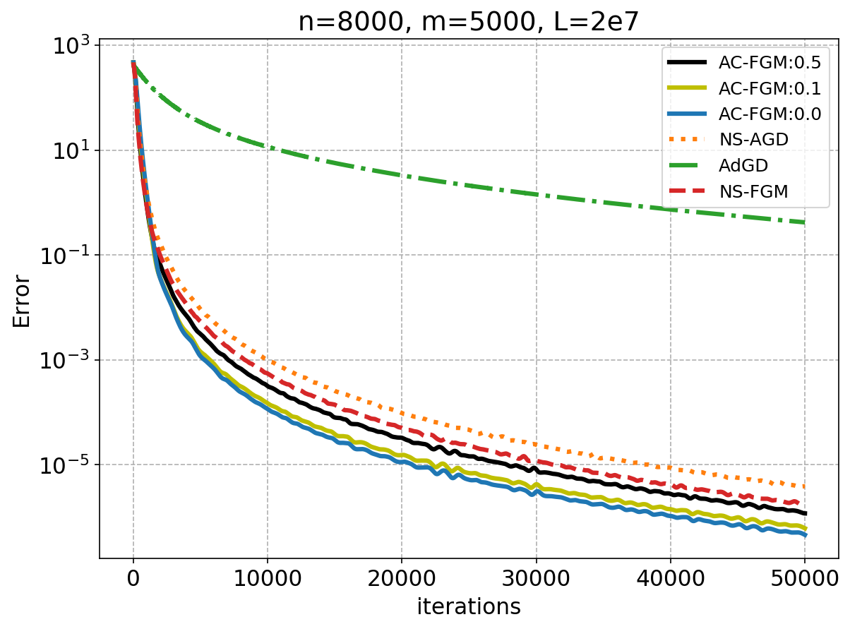
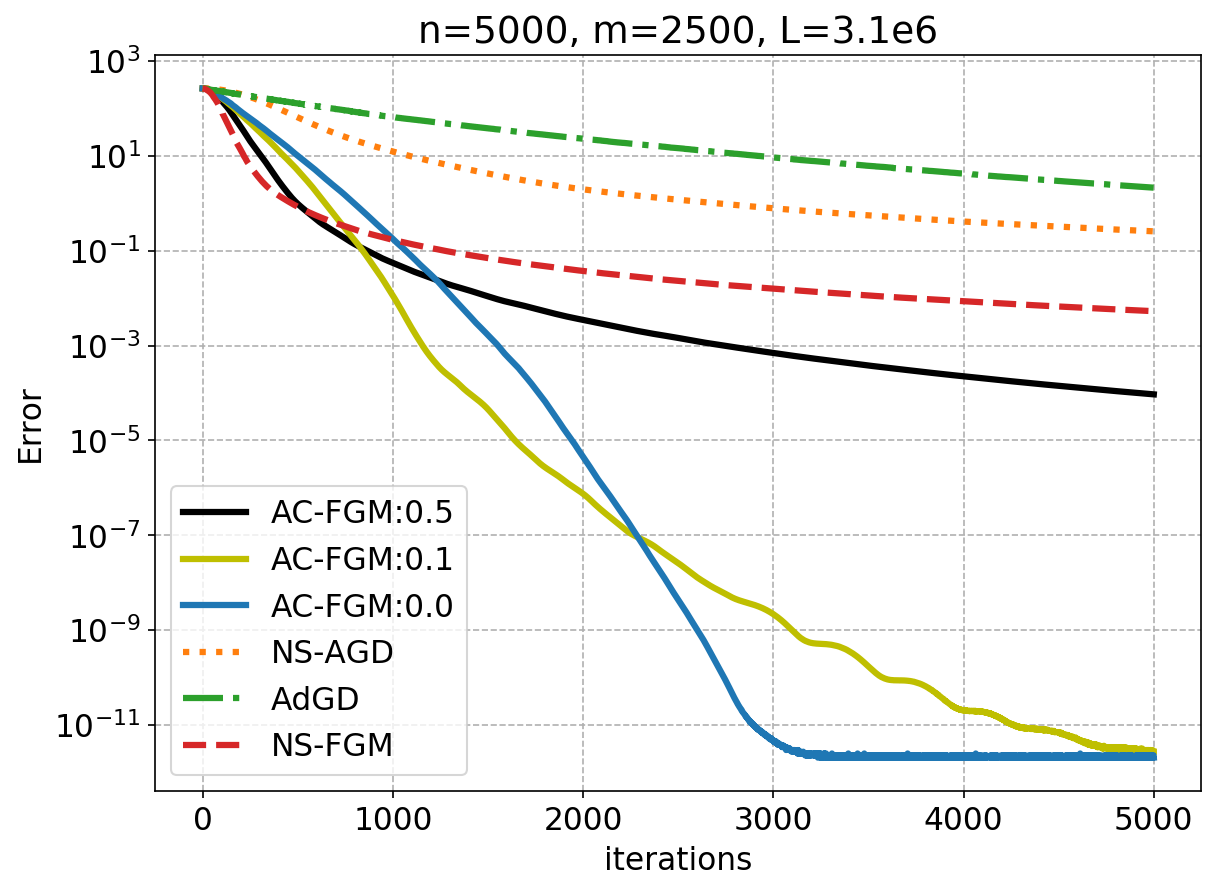
where $L>0$ is the smoothness parameter. This class of instances demonstrate the worst-case convergence behavior $\Omega\left(\sqrt{\tfrac{L\|x_{0}-x^{*}\|^{2}}{\epsilon}}\right)$ of first-order algorithms for smooth convex optimization. In our experiments, we set the Lipschitz constant $L$ to be $2$, the dimension $n$ to be $1000,2000$ and $4000$, and $m=n/2$.

Figure 1: Comparison between AC-FGM, NS-AGD, NS-FGM, and AdGD for problem (5.1).

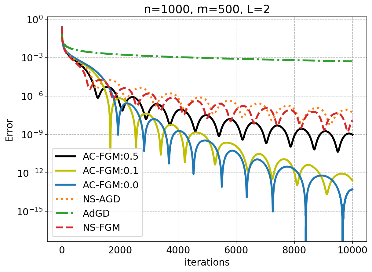
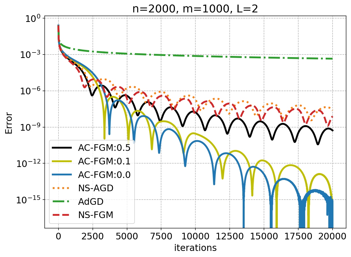
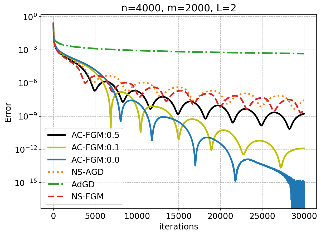
The experiment results are reported in Figure 1. The error in the plot indicates the difference between the objective value and the optimal value in each iteration. Clearly, in the first $m$ iterations, all methods exhibit sublinear convergence due to the existence of the lower bound. Specifically, the accelerated approaches, AC-FGM and NS-FGM, roughly match the convergence rate of NS-AGD, while the AdGD method exhibits a much slower rate, like the vanilla gradient descent. However, after $n$ iterations, AC-FGM, with all different choices of $\alpha$, exhibits more advantageous convergence behavior over NS-AGD as well as NS-FGM. Moreover, we observe that, as we decrease the value of $\alpha$ of AC-FGM, the convergence in the first $n$ iterations is slightly slowed down, but the convergence in the later iterations is accelerated.

5.2 A class of quadratic programming problems

In this subsection, we investigate the performance of AC-FGM on the classical quadratic programming (QP) problem:

$$\min_{\|x\|\leq 1}f(x):=\|Ax-b\|^{2},$$ (5.2)

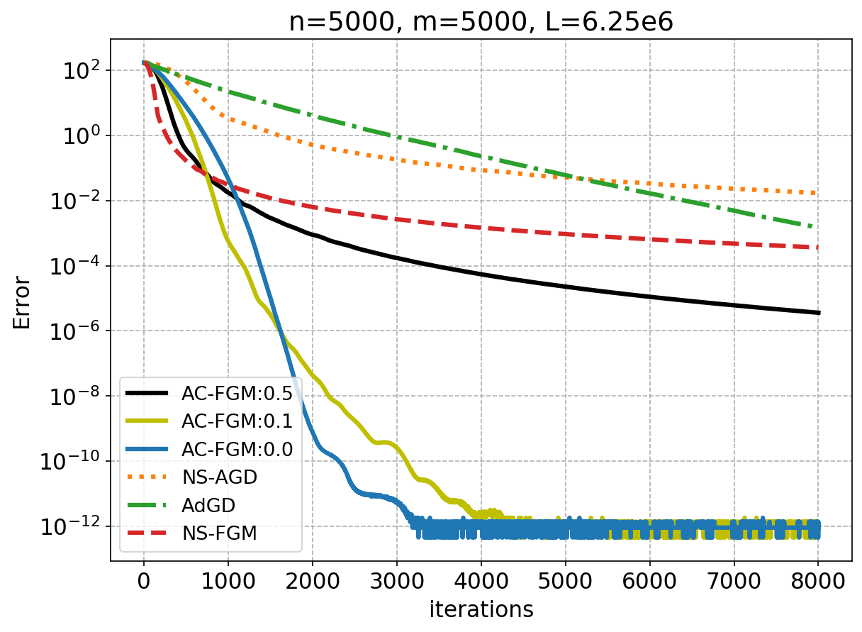
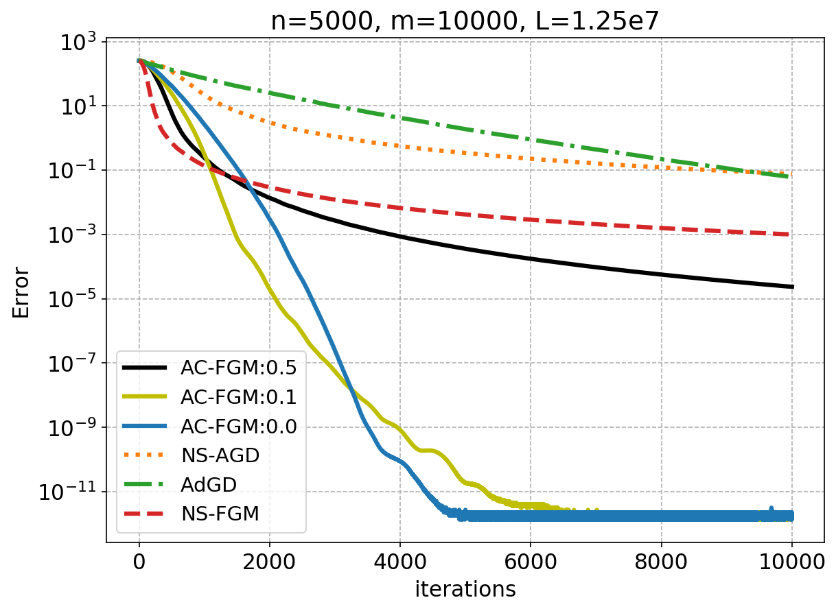
where $A\in\mathbb{R}^{m\times n}$ and $b\in\mathbb{R}^{m}$. In particular, we generate the random instances as follows. First, we randomly choose an optimal solution $x^{*}\in\mathbb{R}^{n}$ in the unit Euclidean ball. Then we generate a matrix $A\in\mathbb{R}^{m\times n}$, where each entry is uniformly distributed in $[0,1]$. At last, we set $b=Ax^{*}$, thus $f(x^{*})=0$. We test the performance of the algorithms on two sets of instances with $n=4000$ and $8000$, respectively. The Lipschitz constants of the first set of instances are in the order of $10^{6}$, while the second set of instances have Lipschitz constants in the order of $10^{7}$. We report the convergence results in Figure 2 and Figure 3 and the computational cost results (CPU time) in Table 1 and Table 2.

Figure 2: Comparison between AC-FGM, NS-AGD, NS-FGM, and AdGD for problem (5.2) with $n=4000$. From left to right $m$ is set to $1000$, $2000$, $3000$, respectively.

Figure 3: Comparison between AC-FGM, NS-AGD, NS-FGM, and AdGD for problem (5.2) with $n=8000$. From left to right $m$ is set to $3000$, $4000$, $5000$, respectively.

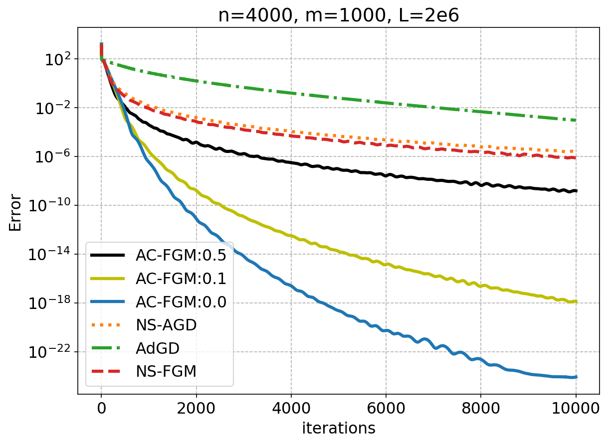
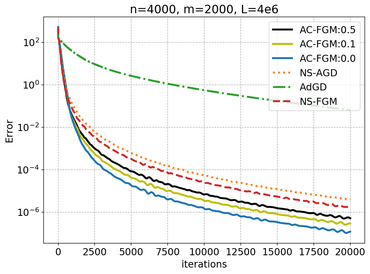
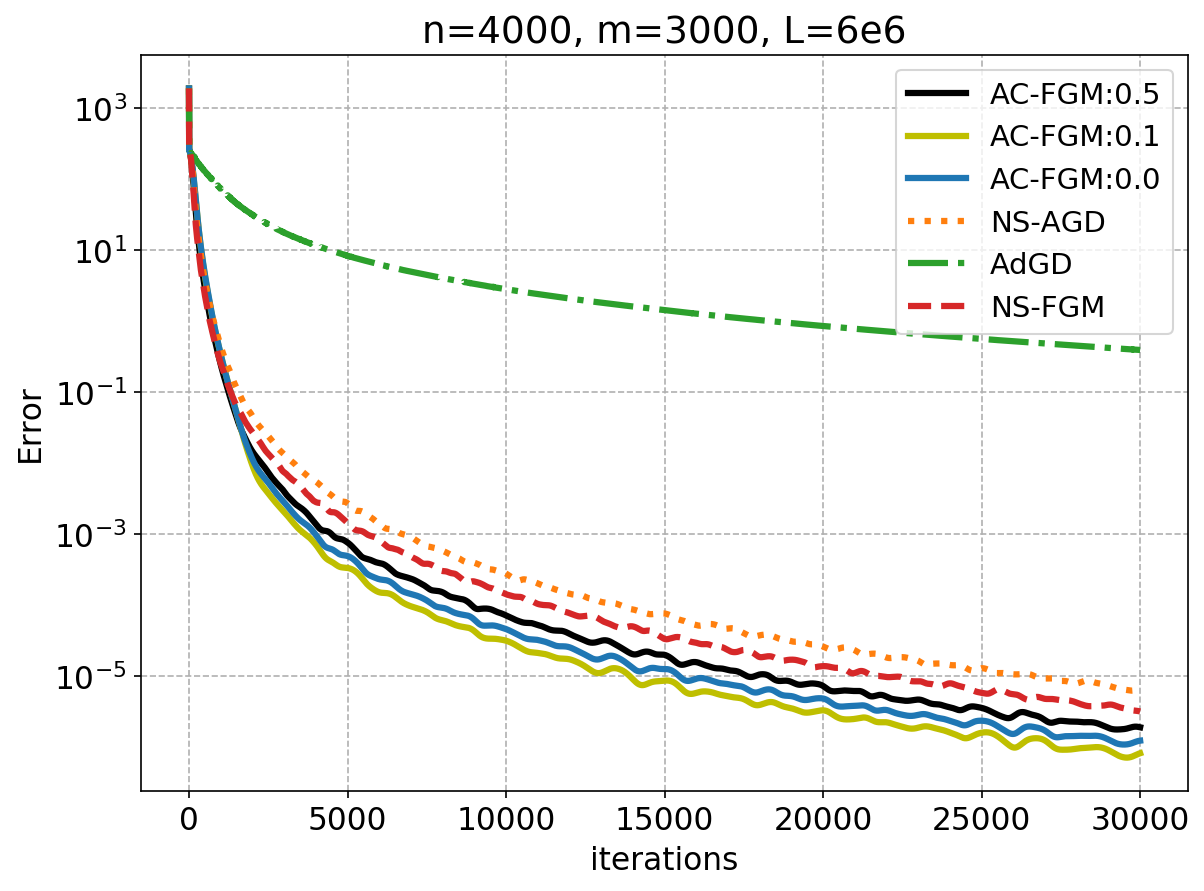
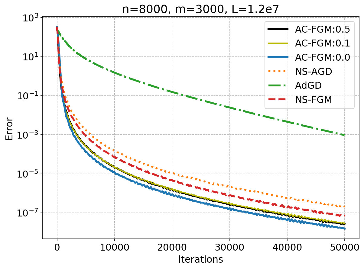
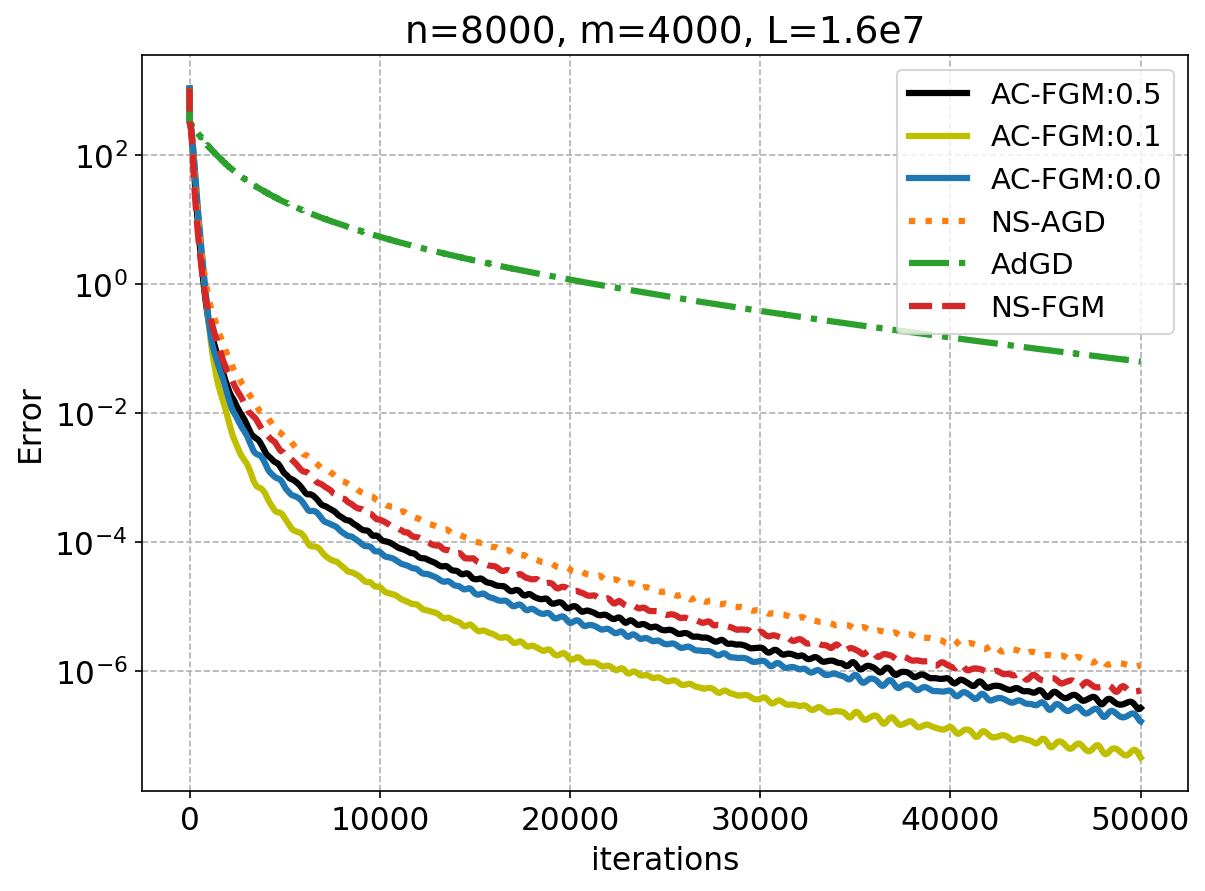
We make the following observations from the results in Figure 2 and Figure 3. First, the accelerated approaches, AC-FGM and NS-FGM, significantly outperform the non-accelerated AdGD method in all the instances. Second, the convergence behavior of NS-FGM closely follows the NS-AGD method, while the AC-FGM largely outperforms the other two accelerated methods in some instances, especially for $n=4000$. Additionally, AC-FGM methods with a smaller choice of $\alpha$, like $0.1$ or $0.0$, exhibit slightly faster convergence than $\alpha=0.5$ in most of the experiments.

Acc	AC-FGM:0.5		AC-FGM:0.1		AC-FGM:0.0		NS-AGD		AdGD		NS-FGM
	Iter	Time	Iter	Time	Iter	Time	Iter	Time	Iter	Time	Iter	Time
$1e-5$	2,075	20.48	893	8.84	805	7.95	7,265	37.34	16,049	112.02	5,765	86.13
$1e-6$	3,309	32.66	1,101	10.90	919	9.08	12,035	61.86	19,235	134.26	9,318	139.21
$1e-7$	4,844	47.81	1,356	13.42	1,111	10.98	18,676	95.99	22,458	156.76	14,504	216.69
$1e-8$	7,237	71.43	1,697	16.80	1,261	12.46	27,706	142.41	25,805	180.12	20,991	313.61
$1e-9$	10,316	101.82	2,059	20.38	1,477	14.59	38,990	200.41	29,111	203.19	28,327	423.21

Table 1: $n=4,000$, $m=1,000$, $L=2\times 10^{6}$. Comparison of the required number of iterations and CPU time in [sec] for achieving different accuracy levels.

Acc	AC-FGM:0.5		AC-FGM:0.1		AC-FGM:0.0		NS-AGD		AdGD		NS-FGM
	Iter	Time	Iter	Time	Iter	Time	Iter	Time	Iter	Time	Iter	Time
$1e-3$	5,232	176.7	3,306	110.9	4,553	152.9	7,772	261.5	107,211	2,799.3	6,472	385.2
$1e-4$	10,501	354.6	6,194	207.9	8,959	301.0	15,204	435.0	142,527	3,721.4	12,566	747.9
$1e-5$	19,764	667.4	12,108	406.4	17,521	588.7	28,717	750.5	178,994	4,673.5	23,454	1,395.9
$1e-6$	36,194	1,222.2	22,924	769.5	32,540	1,093.3	51,768	1,288.8	out of time		41,874	2,494.3
$1e-7$	64,333	2,172.5	41,277	1,385.6	58,584	1,968.4	89,841	2,177.8	out of time		71,486	4,254.8

Table 2: $n=8,000$, $m=4,000$, $L=1.6\times 10^{7}$. Comparison of the required number of iterations and CPU time in [sec] for achieving different accuracy levels.

Table 1 and Table 2 report the computational cost of different algorithms for two problem instances. From the tables, we observe that although NS-FGM requires fewer iterations than NS-AGD to achieve a certain level of accuracy, the CPU time spent by NS-FGM is much longer than NS-AGD due to the high computational cost of line search procedures. In comparison, our AC-FGM approach requires much less CPU time than NS-FGM thanks to its line-search free property. Since AC-FGM also requires much fewer iterations than the other adaptive methods, it significantly saves computational time for reaching different accuracy levels.

5.3 Linear programming

In this subsection, we consider the linear programming (LP) problem

$$\min_{x}~{} c^{T}x$$

s.t. $$Ax=b,~{}~{}x\in\mathbb{R}_{+}^{n},$$ (5.3)

where $A\in\mathbb{R}^{m\times n}$, $b\in\mathbb{R}^{m}$ and $c\in\mathbb{R}^{n}$. The dual problem is

$$\min_{(y,s)}~{} b^{T}y$$

s.t. $$A^{T}y+s=c,~{}~{}s\in\mathbb{R}_{+}^{n}.$$ (5.4)

We assume that the pair of the linear programming problems (5.3) and (5.3) have optimal solutions and the strong duality holds. Then the optimal solution of (5.3) and (5.3) can be found by solving the following constrained system of linear equations:

$$Eu-e =0,~{}u\in\mathcal{U},$$

where $E:=\begin{bmatrix}0&A^{T}&I\\ A&0&0\\ c^{T}&-b^{T}&0\end{bmatrix},~{}~{}u:=\begin{bmatrix}x\\ y\\ s\end{bmatrix},~{}~{}\text{and}~{}~{}e:=\begin{bmatrix}c\\ b\\ 0\end{bmatrix}.$ To solve the system above, we consider solving the following smooth formulation proposed by lan2011primal :

$$\min_{u\in\mathcal{U}}~{}\psi(Eu-e),$$ (5.5)

where

$$\psi((x,y,t)):=\omega_{d}^{2}\|x\|_{2}^{2}+\omega_{p}^{2}\|y\|_{2}^{2}+\omega_{o}^{2}|t|^{2},~{}~{}\forall~{}(x,y,t)\in\mathbb{R}^{n}\times\mathbb{R}^{m}\times\mathbb{R},$$

and $\omega_{d}=\tfrac{1}{\max(1,\|c\|_{2})},~{}~{}\omega_{p}=\tfrac{1}{\max(1,\|b\|_{2})},~{}~{}\omega_{o}=\tfrac{1}{\max(1,\|b\|_{2}+\|c\|_{2})}.$ Notice that our goal is not to propose the best method for solving linear programming problems, but to compare the performance of AC-FGM with other adaptive methods on this important problem class.

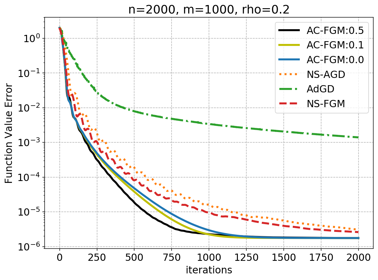
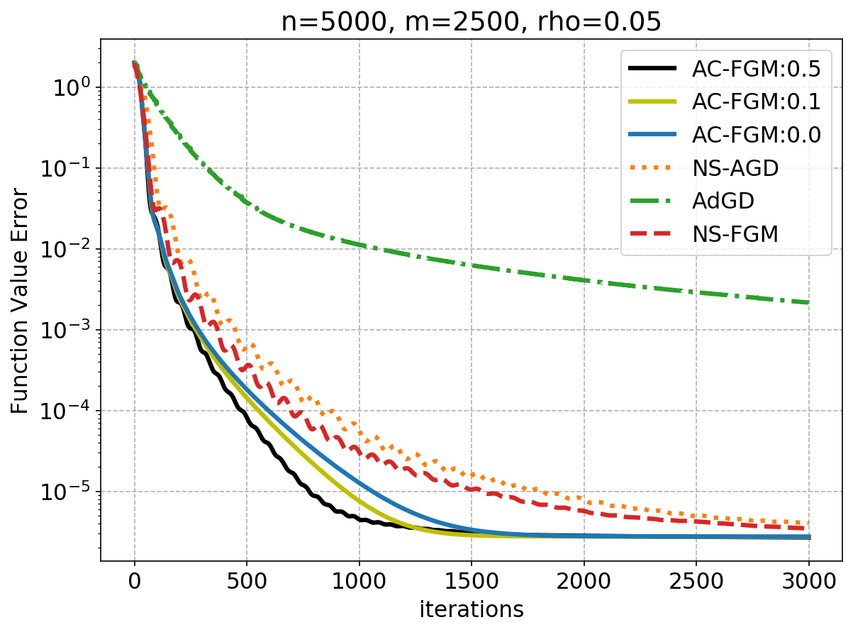
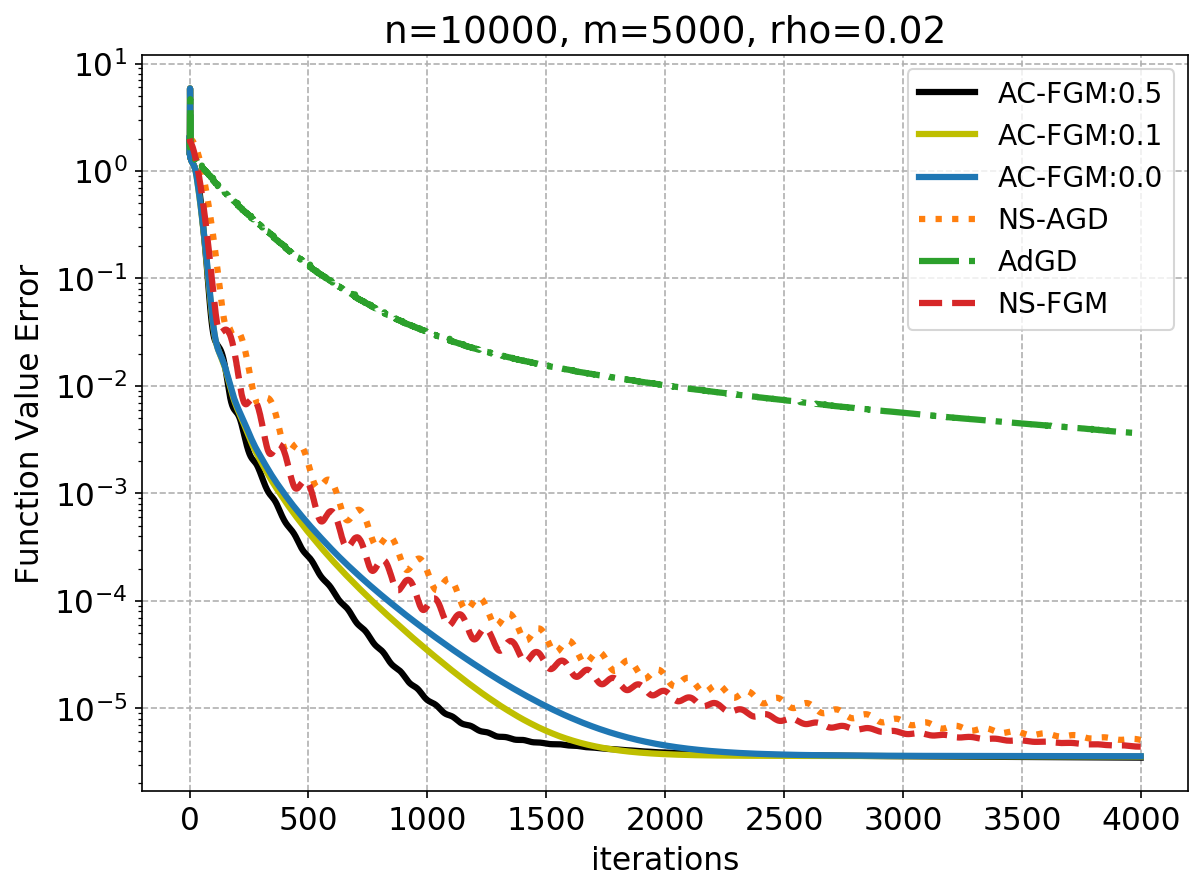
In our experiments, we generate three random LP instances with $n=2000,~{}5000$, and $10000$, respectively. We take $m=n/2$ and set the sparsity level $\rho$ of each instance to be $0.2,~{}0.05$, and $0.02$. For matrix $A\in\mathbb{R}^{m\times n}$, we generate $87.5\%$ of its non-zero entries from a uniform distribution between $[0,1]$ and the other $12.5\%$ from a uniform distribution between $[0,100]$. Then we randomly generate vectors $x^{0},s^{0}\in\mathbb{R}_{+}^{n}$ using the uniform distribution between $[0,1]$, and $y^{0}\in\mathbb{R}^{m}$ using the uniform distribution between $[-1,1]$. By setting $b=Ax^{0}$ and $c=A^{T}y^{0}+s^{0}$, it is clear that the resulting LPs have primal-dual optimal solutions.

We report the convergence results in terms of the objective function value in Figure 4 and the computational cost result of one problem instance in Table 3.

Figure 4: Comparison between AC-FGM, NS-AGD, NS-FGM, and AdGD for problem (5.5). The y-axis represents the function value defined in (5.5).

Acc	AC-FGM:0.5		AC-FGM:0.1		AC-FGM:0.0		NS-AGD		AdGD		NS-FGM
	Iter	Time	Iter	Time	Iter	Time	Iter	Time	Iter	Time	Iter	Time
$1e-3.0$	264	8.13	275	8.38	285	8.83	450	13.99	4,859	128.28	371	18.59
$1e-3.5$	350	10.78	397	12.10	421	13.05	632	18.03	9,506	250.96	479	23.99
$1e-4.0$	478	14.72	553	16.86	597	18.50	830	22.43	out of time		697	34.92
$1e-4.5$	618	19.03	733	22.35	807	25.01	1,116	28.78	out of time		998	50.00
$1e-5.0$	779	23.99	942	28.73	1,059	32.82	1,818	44.36	out of time		1,548	77.55
$1e-5.5$	1,435	44.19	1,334	40.68	1,562	48.42	4,015	93.13	out of time		3,501	175.40

Table 3: $n=5,000$, $m=2,500$, $\rho=0.05$. Comparison of the required number of iterations and CPU time in [sec] for achieving different accuracy levels.

We make the following observations from the results in Figure 4 and Table 3. First, AC-FGM with different choices of $\alpha$ outperforms the other methods, in terms of both the number of iterations and the running time, for achieving different accuracy levels. Second, for this set of problem instances, AC-FGM with $\alpha=0.5$ converges faster than AC-FGM with $\alpha=0.0$ and $0.1$, especially in the first 1000 iterations.

5.4 Sparse logistic regression

In this subsection, we consider a classical convex composite optimization problem, known as the logistic regression with $\ell_{1}$-regularization. In particular, we consider

$$\min_{x\in\mathbb{R}^{n}}~{}\Psi(x):=\textstyle\sum_{i=1}^{m}\log\left(1+\exp(-b_{i}\langle a_{i},x\rangle)\right)+\gamma\|x\|_{1},$$ (5.6)

where $\gamma>0$ is the regularization parameter, and $a_{i}\in\mathbb{R}^{n}$ and $b_{i}\in\{-1,1\}$ represent the feature vector and the binary index of each sample, respectively. This problem can be viewed as a composite optimization of a smooth function and a nonsmooth function, i.e.,

$$\Psi(x)=f(x)+h(x)=\tilde{f}(Kx)+h(x),$$

where $\tilde{f}(y)=\textstyle\sum_{i=1}^{m}\log(1+\exp(y_{i}))$, $h(x)=\gamma\|x\|_{1}$, and $K\in\mathbb{R}^{m\times n}$ satisfies $K_{i,j}=-a_{i}^{(j)}b_{i}$. Clearly, the Lipschitz constant of $\tilde{f}$ is bounded by $\tfrac{1}{4}$, thus the Lipschitz constant of $f$ can be upper bounded by $L=\tfrac{1}{4}\lambda_{\max}(K^{T}K)$. It is also noteworthy that the local smoothness constant of $\tilde{f}$ can be much smaller than $\tfrac{1}{4}$ as $y$ gets far away from the origin. Therefore, if we set the origin $\mathbf{0}$ as the initial point $x_{0}$, the adaptive algorithms that can take advantage of the local smoothness level may have much faster convergence than the non-adaptive algorithms. Moreover, we take the common rule $\gamma=0.005\|A^{T}b\|_{\infty}$ for all sets of experiments.

In the first set of experiments, we construct random instances as follows. First, we generate each entry of matrix $A\in\mathbb{R}^{m\times n}$ with a uniform distribution in $[0,1]$. Then we generate the vector $b\in\mathbb{R}^{m}$, where each entry follows a Bernoulli distribution between $\{-1,1\}$. We set $n=5000$ and $m=2500$, $5000$, $10000$, respectively. The Lipschitz constants of these instances are in the order of $10^{6}$ or $10^{7}$, making them challenging for first-order methods.

Figure 5: Comparison between AC-FGM, NS-AGD, NS-FGM, and AdGD for problem (5.6) on random instances with $n=5000$. From left to right $m$ is set to $2500$, $5000$, $10000$, respectively.

From Figure 5, we can see that NS-FGM slightly outperforms the other methods at the very beginning of all the experiments, but the AC-FGM methods quickly catch up in less than $1000$ iterations and then significantly outperforms the other methods. Specifically, the progress of NS-FGM slows down due to the conservative choice of stepsizes, but the novel adaptive stepsize rule of AC-FGM (Corollary 2) takes advantage of the structural property of $\tilde{f}$, thus leading to more efficient convergence. Moreover, as we decrease $\alpha$ in AC-FGM, the convergence slightly slows down in the first few iterations but is significantly accelerated in the following iterations. Notice that the AdGD approach also makes consistent progress and catches up with NS-AGD and NS-FGM eventually.

Acc	AC-FGM:0.5		AC-FGM:0.1		AC-FGM:0.0		NS-AGD		AdGD		NS-FGM
	Iter	Time	Iter	Time	Iter	Time	Iter	Time	Iter	Time	Iter	Time
$1e-2$	1,124	21.8	837	16.2	1,113	21.5	10,195	110.2	6,408	79.5	1,623	46.0
$1e-3$	1,938	37.6	956	18.5	1,261	24.4	30,517	329.9	8,322	103.2	4,823	136.7
$1e-4$	3,435	66.6	1,180	22.9	1,383	26.7	95,453	1,031.8	10,350	128.3	15,241	431.9
$1e-5$	6,155	119.3	1,345	26.1	1,501	29.0	out of time		12,432	154.2	out of time
$1e-6$	11,081	214.7	1,697	31.3	1,619	31.3	out of time		14,504	179.8	out of time
$1e-7$	19,856	384.8	2,059	36.7	1,733	33.5	out of time		16,685	206.9	out of time

Table 4: $n=5,000$, $m=5,000$, $L=6.25\times 10^{6}$. Comparison of the required number of iterations and CPU time in [sec] for achieving different accuracy levels.

Table 4 reports the computational cost of different algorithms for the problem instance $n=5,000,m=5,000$. Clearly, AC-FGM with $\alpha=0.0$ and $\alpha=0.1$ consistently outperforms the other methods, in terms of both the number of iterations and CPU time, for achieving different levels of accuracy.

Figure 6: Comparison between AC-FGM, NS-AGD, NS-FGM, and AdGD for problem (5.6) on rcv$\_$train.binary (left) and real$-$sim (right) in LIBSVM.

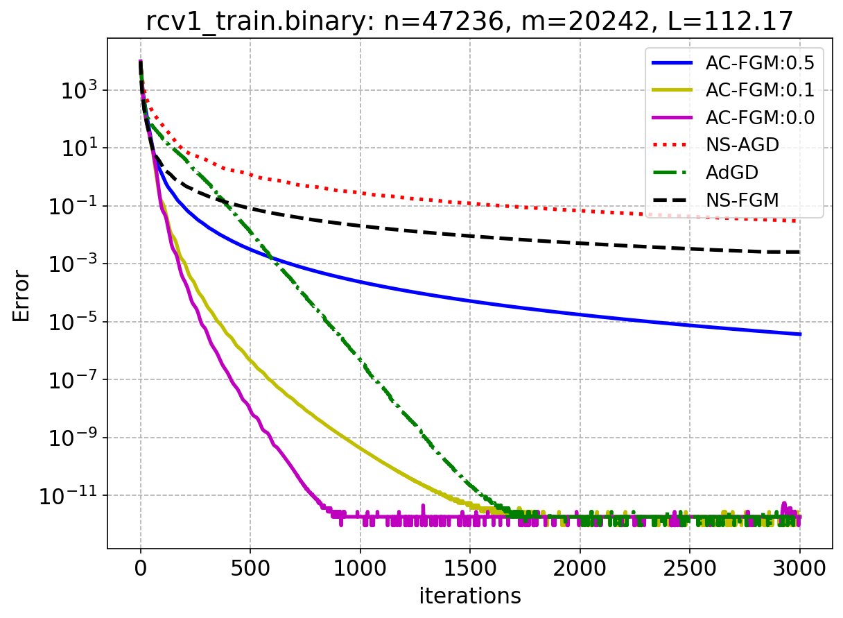
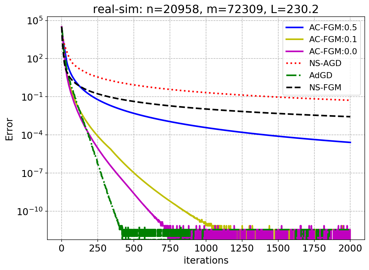
At last, we report the results on two real-world datasets, i.e., rcv$\_$train.binary and real$-$sim in LIBSVM. The first one is over-parametrized with $n=47,236$ and $m=20,242$, while the second one has $n=20,958$ and $m=72,309$. Due to the sparsity of the features, both instances have a relatively low worst-case Lipschitz constant, i.e., 112.17 and 230.2. From Figure 6, we observe that AC-FGM, with $\alpha=0.0$ and $0.1$, and AdGD achieve efficient convergence compared with the other approaches, due to the adaptive choices of the stepsizes that take advantage of the local curvature of the objective function. However, since the Lipschitz constants are relatively small in these instances, AC-FGM is not significantly more advantageous than AdGD.

6 Concluding remarks

In summary, we design a novel accelerated gradient decent type algorithm, AC-FGM, for convex optimization. We first show that AC-FGM is fully problem parameter free, line-search free, and optimal for smooth convex problems. Then we extend AC-FGM to solve convex problems with Hölder continuous gradients and demonstrate its uniform optimality for all smooth, weakly smooth, and nonsmooth objectives. We further extend the uniformly optimal results to the composite optimization setting. At last, we present some numerical experiments, where AC-FGM appears to be much more advantageous over the previously developed parameter-free methods on a wide range of testing problems.