Convolution quadratures based on block generalized Adams methods

Abstract

This paper studies a class of convolution quadratures, well-known numerical methods for calculation of convolution integrals. In contrast to the existing counterpart, which uses the linear multistep formula or Runge-Kutta method, we employ the block generalized Adams method to discretize the underlying initial value problem. Similar to the convolution quadrature method based on the linear multistep formula, the proposed method can also be implemented on an equispaced grid. In addition, the proposed approach is as stable as the convolution quadrature based on the Runge-Kutta method, which indicates that it can accurately solve a wide range of problems without becoming unstable. We provide a detailed convergence analysis for the proposed convolution quadrature method and numerically illustrate our theoretical findings for convolution integrals with smooth and weakly singular kernels.

1 Introduction

Convolution integrals (CIs) have a number of applications in computational practice, such as time-domain boundary integral equations [3], Volterra integral equations of convolution-type [8], fractional differential equations [15, 25] and Maxwell’s equations [26]. In this paper, we investigate the numerical evaluation of the following CI

(1) $$\mathrm{I}[k,g](t)=\int_{0}^{t}k(s)g(t-s)ds,~{}t\in[0,T],$$

where $g$ is a given smooth function. When the kernel function $k$ itself is known previously, many efficient approaches can be used to compute CI (1), for example, the convolution spline method [10] and spectral method based on orthogonal polynomial convolution matrices [27, 28]. However, if the Laplace transform $K$ of the kernel function $k$ is known, then the convolution quadrature (CQ), which was proposed by Lubich in [18, 19, 20], will be a popular choice for calculation of CI (1).

CQs are typically constructed by converting the calculation of an integral to the numerical discretization of an initial value problem. Suppose the kernel function $k$ has a sectorial Laplace transform $K,$ that is, $K$ is analytic in a sector

$$\mathbb{C}_{\varphi}:=\{\lambda\in\mathbb{C}:|\arg(\lambda-c)|<\pi-\varphi\}$$

with $\varphi\in(0,\pi/2),c\in\mathbb{R}.$ In addition, assume $|K(\lambda)|$ is bounded by $M|\lambda|^{-\mu}$ for $\lambda\in\mathbb{C}_{\varphi}$ with a constant $M$ and $\mu>0.$ Noting that

(2) $$k(t)=\frac{1}{2\pi\mathrm{i}}\int_{\Gamma}K(\lambda)\mathrm{e}^{\lambda t}d\lambda,~{}~{}t>0,$$

where $\Gamma$ is a curve locating in the analytic region of $K,$ parallel to its boundary and oriented with increasing imaginary part [21], we obtain

(3) $$\mathrm{I}[k,g](t)=\frac{1}{2\pi\mathrm{i}}\int_{\Gamma}K(\lambda)\int_{0}^{t}\mathrm{e}^{\lambda s}g(t-s)dsd\lambda.$$

Letting $y(t)=\int_{0}^{t}\mathrm{e}^{\lambda s}g(t-s)ds,$ we obtain the following initial value problem (IVP) for the ordinary differential equation (ODE):

(6) $$\left\{\begin{array}[]{l}y^{\prime}(t)=\lambda y(t)+g(t),~{}~{}t>0,\\ y(0)=0.\end{array}\right.$$

The discretization for CI (1) then consists of two steps: approximating IVP (6) using time-stepping methods, and computing contour integrals.

In the literature, two types of ODE solvers for IVP (6) have been extensively investigated. Lubich’s pioneering work in [18, 19] used linear multistep formulas to solve IVP (6) and developed the linear multistep convolution quadrature (LMCQ) method. Convergence analysis showed that LMCQ has the same convergence rate as the underlying linear multistep formula, once correction terms are added. Define the uniform grid $\mathbb{X}_{N}$ with the stepsize $h=T/N$ by

$$\mathbb{X}_{N}:=\{t^{n}=nh,~{}n=0,1,\cdots,N\}.$$

Letting $\delta(\zeta)$ be the quotient of generating polynomials of the linear multistep formula, we obtain LMCQ in the form of:

(7) $$\mathrm{I}[k,g](t^{n})\approx\sum_{j=0}^{n}\omega_{j}g(t^{n-j}),$$

where quadrature weights $\omega_{j}$s are usually obtained by numerically computing contour integrals, as they are simply the coefficients of the Taylor expansion of $K.$ LMCQ can be implemented on a uniform grid, which makes it a promising method for the time discretization of fractional differential equations (see [9, 15, 16]). However, since the stability of the discretization of IVP (6) heavily affects the convergence property of the resulting CQ, the commonly-used LMCQ is based on the low-order formulas, for example, from the backward difference formula of order 2 (BDF2CQ) with $\delta(\zeta)=\frac{3}{2}-2\zeta+\frac{1}{2}\zeta^{2}$ (see [9]) to the trapezoid rule with $\delta(\zeta)=2\frac{1-\zeta}{1+\zeta}$ (see [5, 11]). By contrast, Runge-Kutta methods discretizing IVP (6) yield arbitrarily accurate and stable CQs for sufficiently smooth functions $g$ in CI (1) (see [20]). To define CQ based on the Runge-Kutta method (RKCQ), we first need to select the internal points,

$$t^{n}+c_{1}h,t^{n}+c_{2}h,\cdots,t^{n}+c_{m}h,$$

which locate in the subinterval $[t^{n},t^{n+1}]$ with $n=0,1,\cdots,N-1.$ Then, making use of Butcher’s tableau

$$\mathbb{B}=\left(\begin{array}[]{c}b_{1}\\ b_{2}\\ \vdots\\ b_{m}\\ \end{array}\right),~{}\mathbb{I}=\left(\begin{array}[]{c}1\\ 1\\ \vdots\\ 1\\ \end{array}\right),~{}\mathbb{A}=\left(\begin{array}[]{cccc}a_{11}&a_{12}&\cdots&a_{1m}\\ a_{21}&a_{22}&\cdots&a_{2m}\\ \vdots&\vdots&&\vdots\\ a_{m1}&a_{m2}&\cdots&a_{mm}\\ \end{array}\right),$$

we obtain the Runge-Kutta differentiation symbol

$$\Delta(\zeta)=\left(\frac{\zeta}{1-\zeta}\mathbb{I}\mathbb{B}^{T}+\mathbb{A}\right)^{-1}.$$

Subsequently, for $n=0,1,\cdots,N-1,$ RKCQ is defined by

(16) $$\left(\begin{array}[]{c}\mathrm{I}[k,g](t^{n}+c_{1}h)\\ \mathrm{I}[k,g](t^{n}+c_{2}h)\\ \vdots\\ \mathrm{I}[k,g](t^{n}+c_{m}h)\\ \end{array}\right)\approx\sum_{j=0}^{n}\mathbb{W}_{n-j}\left(\begin{array}[]{c}g(t^{j}+c_{1}h)\\ g(t^{j}+c_{2}h)\\ \vdots\\ g(t^{j}+c_{m}h)\\ \end{array}\right),$$

where the matrices $\mathbb{W}_{j}$s of quadrature weights are determined by $K(\Delta(\zeta)/h)=\sum_{j=0}^{\infty}\mathbb{W}_{j}\zeta^{j}.$ High-order RKCQ can be developed by properly selecting the parameters $c_{i}$s, since $A-$stable Runge-Kutta methods of arbitrary order are available. As a result of its good stability, high-order RKCQ has a wider application than LMCQ, particularly in numerical studies on the wave equation (see [22, 23, 24]). In addition, the fast implementation and variable time stepping techniques, which are important for computing CI (1) efficiently and accurately, have been extensively studied in [12] and [17], respectively. Recently, Banjai and Ferrari in [4] show that RKCQ can exhibit superconvergence when the parameters $c_{i}$s are chosen to be Gauss points.

This paper proposes to develop high-order and stable CQs on a uniform grid. In contrast to the existing LMCQ and RKCQ, we employ the block generalized Adams method. The idea for this approach comes from numerical solutions to ODEs using the boundary value method (see [6, 13, 14]), which has been shown to improve the stability of numerical solutions. The proposed CQ uses a matrix-valued differentiation symbol, which is similar to RKCQ, and allows for the easy adjustment of the matrix size in its differentiation symbol, which is important for improving the stability of the long-time integration. The remaining part is organized as follows. Section 2 introduces the convolution quadrature based on the block generalized Adams method (BGACQ). In Section 3, the convergence property of BGACQ is established under some regularization conditions. Section 4 presents numerical experiments to verify the convergence rate and stability of the proposed method. Some conclusions are given in Section 5.

2 Formulation of BGACQ

In this section, we present the formulation of BGACQ, beginning with a review of the block generalized Adams method for solving IVP (6), as BGACQ is based on this approach.

Firstly, with the uniform grid $\mathbb{X}_{N}$ in hand, we define a fine grid over $[t^{n},t^{n+1}],$ that is,

$$\mathbf{X}_{m}^{n}:=\{t^{n}_{j}:t^{n}_{j}=t^{n}+jh/m,~{}j=0,1,\cdots,m\}.$$

For each subinterval $[t^{n},t^{n+1}],$ integration of both sides of IVP (6) from $t^{n}_{j}$ to $t^{n}_{j+1}$ with $j=0,1,\cdots,m-1$ gives

(17) $$y(t_{j+1}^{n})-y(t_{j}^{n})=\int_{t_{j}^{n}}^{t_{j+1}^{n}}(\lambda y(s)+g(s))ds.$$

Secondly, we construct the local interplant for $\lambda y(s)+g(s)$ that arises on the right-hand side of Eq. (17). For any given nonnegative integers $k_{1}$ and $k_{2},$ define the local fundamental functions

$$\phi_{i}^{k_{1},k_{2}}(s)=\prod_{l=-k_{1},l\neq i}^{k_{2}+1}\frac{s-l}{i-l},~{}i=-k_{1},\cdots,k_{2}+1.$$

To simplify the notation, we define the function $f(t):=\lambda y(t)+g(t)$ and its piecewise interpolation polynomial $f_{N}(t),$ which approximates $f(t)$ on the uniform grid $\mathbf{X}_{m}^{n}.$ We discuss the approximation in three cases, that is,

• $t\in[t^{n}_{0},t^{n}_{k_{1}}];$

• $t\in[t^{n}_{j},t^{n}_{j+1}]$ with $j=k_{1},k_{1}+1,\cdots,m-k_{2}-1;$

• $t\in[t^{n}_{m-k_{2}},t^{n}_{m}].$

For any $t\in[t^{n}_{0},t^{n}_{k_{1}}],$ we approximate $f(t)$ by the interpolation polynomial in the form of

(18) $$f(t)=f(t_{k_{1}}^{n}+sh/m)\approx f_{N}(t_{k_{1}}^{n}+sh/m)=\sum_{i=-k_{1}}^{k_{2}+1}f(t_{k_{1}+i}^{n})\phi_{i}^{k_{1},k_{2}}(s),~{}~{}s\in[-k_{1},0].$$

For any $t\in[t^{n}_{j},t^{n}_{j+1}]$ with $j=k_{1},k_{1}+1,\cdots,m-k_{2}-1,$ $f(t)$ is approximated by

(19) $$f(t)=f(t_{j}^{n}+sh/m)\approx f_{N}(t_{j}^{n}+sh/m)=\sum_{i=-k_{1}}^{k_{2}+1}f(t_{j+i}^{n})\phi_{i}^{k_{1},k_{2}}(s),~{}~{}s\in[0,1].$$

In the case of $t\in[t^{n}_{m-k_{2}},t^{n}_{m}],$ we approximate $f(t)$ by

(20) $$f(t)=f(t_{m-k_{2}-1}^{n}+sh/m)\approx f_{N}(t_{m-k_{2}-1}^{n}+sh/m)=\sum_{i=-k_{1}}^{k_{2}+1}f(t_{m-k_{2}-1+i}^{n})\phi_{i}^{k_{1},k_{2}}(s)$$

with $s\in[1,k_{2}+1].$ As a result, we obtain the quadrature rule for $\int_{t_{j}^{n}}^{t_{j+1}^{n}}f(t)dt,$ that is,

(24) $$\int_{t_{j}^{n}}^{t_{j+1}^{n}}f(t)dt\approx\left\{\begin{array}[]{l}\frac{h}{m}\sum_{i=-k_{1}}^{k_{2}+1}f(t_{k_{1}+i}^{n})\int_{j-k_{1}}^{j-k_{1}+1}\phi_{i}^{k_{1},k_{2}}(s)ds,~{}~{}j=0,\cdots,k_{1}-1,\\ \frac{h}{m}\sum_{i=-k_{1}}^{k_{2}+1}f(t_{j+i}^{n})\int_{0}^{1}\phi_{i}^{k_{1},k_{2}}(s)ds,~{}~{}j=k_{1},\cdots,m-k_{2}-1,\\ \frac{h}{m}\sum_{i=-k_{1}}^{k_{2}+1}f(t_{m-k_{2}-1+i}^{n})\int_{j-m+k_{2}+1}^{j-m+k_{2}+2}\phi_{i}^{k_{1},k_{2}}(s)ds,~{}~{}j=m-k_{2},\cdots,m-1.\end{array}\right.$$

Finally, letting $\textsc{Mom}_{p,i}=\frac{1}{m}\int_{p}^{p+1}\phi_{i}^{k_{1},k_{2}}(s)ds,$ we define the matrices of dimension $m\times m$ as follows:

$$\mathbf{A}=(a_{ij}),~{}~{}\mathbf{B}=(b_{ij}),~{}~{}\mathbf{C}=(c_{ij}),~{}~{}\mathbf{D}=(d_{ij}),$$

where

$$a_{ij}=\left\{\begin{array}[]{l}\textsc{Mom}_{i-k_{1}-1,j-k_{1}},~{}~{}i=1,\cdots,k_{1}+1,~{}j=1,\cdots,k_{1}+k_{2}+1,\\ \textsc{Mom}_{0,j-i+1},~{}~{}i=k_{1}+2,\cdots,m-k_{2},~{}j=i-k_{1}-1,\cdots,i+k_{2},\\ \textsc{Mom}_{i-m+k_{2},j-m+k_{2}+1},~{}~{}i=m-k_{2}+1,\cdots,m,~{}j=m-k_{1}-k_{2}-1,\cdots,m,\\ 0,~{}~{}\mathrm{others},\end{array}\right.$$

$$b_{ij}=\left\{\begin{array}[]{l}1,~{}~{}i=j,\\ -1,~{}~{}i=j+1,~{}j=1,\cdots,m-1,\\ 0,~{}~{}\mathrm{others},\end{array}\right.c_{ij}=\left\{\begin{array}[]{l}1,~{}~{}i=1,~{}j=m,\\ 0,~{}~{}\mathrm{others},\end{array}\right.$$

$$d_{ij}=\left\{\begin{array}[]{l}\textsc{Mom}_{i-k_{1}-1,-k_{1}},~{}~{}i=1,\cdots,k_{1}+1,~{}j=m,\\ 0,~{}~{}\mathrm{others}.\end{array}\right.$$

To conclude, the block generalized Adams method discretizes Eq. (17) into

(25) $$\mathbf{B}\mathbf{Y}_{n}-\mathbf{C}\mathbf{Y}_{n-1}=h\lambda\mathbf{D}\mathbf{Y}_{n-1}+h\lambda\mathbf{A}\mathbf{Y}_{n}+h\mathbf{D}\mathbf{G}_{n-1}+h\mathbf{A}\mathbf{G}_{n},~{}n=0,\cdots,N-1,$$

where $\mathbf{G}_{n}=(g(t_{1}^{n})~{}~{}\cdots~{}~{}g(t_{m}^{n}))^{T},$ $\mathbf{Y}_{n}=(y^{n}_{1}~{}~{}\cdots~{}~{}y^{n}_{m})^{T}$ denotes the approximation to $\mathbf{Y}_{n}^{ref}=(y(t_{1}^{n})~{}~{}\cdots~{}~{}y(t_{m}^{n}))^{T},$ and $\mathbf{G}_{-1}$ and $\mathbf{Y}_{-1}$ are denoted as the $m\times 1$ null vectors. In order to guarantee that Eq. (25) makes sense, the identity $g(0)=0$ should hold on. From now on, we assume $g(0)=0$, unless there are special circumstances.

It is noted that matrices in Eq. (25) are determined by the parameters $k_{1},k_{2},m,$ and independent of $N.$ Therefore, we can analyze the property of the block generalized Adams method as quadrature nodes increases once the the parameters $k_{1},k_{2},m$ are given previously. In Table 1 and Figure 1, we show the spectral radius of $\mathbf{A}^{-1}\mathbf{D}$ and eigenvalues of $\mathbf{A}^{-1}\mathbf{B},$ respectively. We find that the spectral radius of $\mathbf{A}^{-1}\mathbf{D}$ is less than $1$ and decays as $m$ enlarges, which ensures that the block generalized Adams method is stable and convergent. Besides, it is found that the real part of eigenvalues of $\mathbf{A}^{-1}\mathbf{B}$ is positive in these cases. Meanwhile, increasing the parameter $m$ causes the eigenvalues of $\mathbf{A}^{-1}\mathbf{B}$ to move away from the imaginary axis, which guarantees that the discrete differentiation symbol is well-defined. We state the following assumption for the block generalized Adams method, which is required in the construction of CQ.

Assumption 2.1.

Given the parameters $k_{1},k_{2},m,$ the matrices $\mathbf{A},\mathbf{B},\mathbf{D}$ arising in the block generalized Adams method satisfy:

• The spectral radius of $\mathbf{A}^{-1}\mathbf{D}$ is less than $1;$

• Eigenvalues of $\mathbf{A}^{-1}\mathbf{B}$ locate in $\mathbb{C}_{\varphi};$

• Zero is not the eigenvalue of $\mathbf{A}^{-1}\mathbf{B}.$

Table 1: The spectral radius of $\mathbf{A}^{-1}\mathbf{D}.$

  $m$ $(k_{1},k_{2})=(0,1)$ $(k_{1},k_{2})=(0,2)$ $(k_{1},k_{2})=(1,2)$ $(k_{1},k_{2})=(1,3)$ 10 $1.3\times 10^{-2}$ $2.4\times 10^{-3}$ $1.5\times 10^{-1}$ $6.4\times 10^{-2}$ 20 $6.0\times 10^{-5}$ $4.5\times 10^{-7}$ $5.6\times 10^{-3}$ $2.4\times 10^{-4}$ 30 $2.7\times 10^{-7}$ $8.1\times 10^{-11}$ $2.2\times 10^{-4}$ $8.7\times 10^{-7}$ 40 $1.2\times 10^{-9}$ $1.5\times 10^{-14}$ $8.5\times 10^{-6}$ $3.3\times 10^{-9}$ 50 $5.5\times 10^{-12}$ $2.7\times 10^{-18}$ $3.3\times 10^{-7}$ $1.2\times 10^{-11}$  

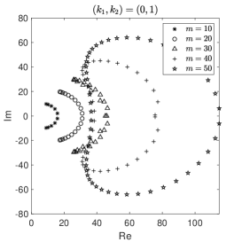
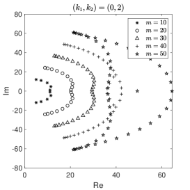
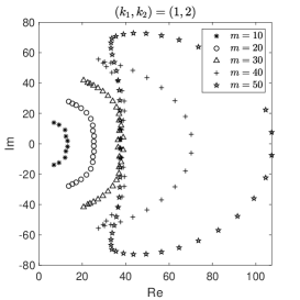
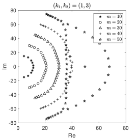
Fig. 1: Distributions of eigenvalues of $\mathbf{A}^{-1}\mathbf{B}.$

Let us now consider the formulation of CQ with the help of the above block generalized Adams method. Multiplying both sides of Eq. (25) by $\zeta^{n}$ and doing summation over $n$ from $0$ to $\infty$ give

(26) $$(\mathbf{B}-h\lambda\mathbf{A})\mathbf{Y}(\zeta)-\zeta(\mathbf{C}+\lambda h\mathbf{D})\mathbf{Y}(\zeta)=h(\mathbf{A}+\zeta\mathbf{D})\mathbf{G}(\zeta),$$

where $\mathbf{Y}(\zeta)=\sum_{n=0}^{\infty}\mathbf{Y}_{n}\zeta^{n},$ $\mathbf{G}(\zeta)=\sum_{n=0}^{\infty}\mathbf{G}_{n}\zeta^{n}.$ It can be found by a direct calculation that if Assumption 2.1 is satisfied, $\mathbf{A}+\zeta\mathbf{D}$ is invertible for any $\zeta$ such that $|\zeta|<1.$ We can now safely define the block generalized Adams differential symbol by $\Delta(\zeta)=(\mathbf{A}+\zeta\mathbf{D})^{-1}(\mathbf{B}-\zeta\mathbf{C}).$ Rearranging Eq. (26) leads to

(27) $$\mathbf{Y}(\zeta)=\left(\Delta(\zeta)/h-\lambda\mathbf{E}_{m}\right)^{-1}\mathbf{G}(\zeta),$$

where $\mathbf{E}_{m}$ denotes the $m\times m$ identity matrix.

On the other hand, consider the homogeneous version of Eq. (25), that is,

(28) $$(\mathbf{B}-h\lambda\mathbf{A})\mathbf{Y}_{n}=(\mathbf{C}+h\lambda\mathbf{D})\mathbf{Y}_{n-1}.$$

If $\mathbf{B}-h\lambda\mathbf{A}$ is invertible, we obtain by a repeated iteration that

(29) $$y^{n}_{m}=\mathbf{R}(h\lambda)y^{n-1}_{m},$$

where $\mathbf{R}(z)$ defined by $\mathbf{R}(z):=\mathbf{e}_{m}^{T}(\mathbf{B}-z\mathbf{A})^{-1}(\mathbf{C}+z\mathbf{D})\mathbf{e}_{m}$ is called to be the stability function of the block generalized Adams method, and $\mathbf{e}_{m}$ denotes the $m\times 1$ column vector with all elements being zero except for the last element, which is one. Then for any $z$ locating in the left part of the complex plane, the block generalized Adams method is stable at $z$ if $\mathbf{B}-z\mathbf{A}$ is nonsingular and $|\mathbf{R}(z)|\leq 1.$ Furthermore, the set consisting of the stable points is called to be the stability domain of the block generalized Adams method. If the block generalized Adams method is stable in the sector $\mathbb{\hat{C}}_{\theta}:=\{\lambda\in\mathbb{C}:|\arg(-\lambda)|\leq\theta,\lambda\neq 0\},$ then it is called to be $A(\theta)-$stable. Meanwhile, the block generalized Adams method is called to be $A-$stable if it is stable in $\mathbb{\hat{C}}_{\pi/2}.$ In Figures 2 and 3, we show the stability domains of several kinds of block generalized Adams methods. It is found that this method is $A-$stable in the case of $0\leq k_{2}-k_{1}\leq 2.$ In the cases where $k_{2}-k_{1}<0$ or $k_{2}-k_{1}>2,$ its stability domain is a sector.

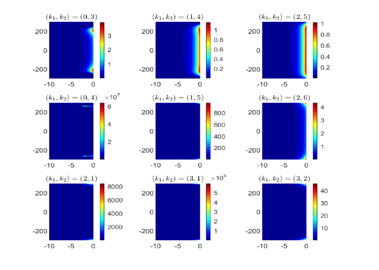
Fig. 2: Stability domains of the block generalized Adams method with $k_{2}<k_{1}$ or $k_{2}-k_{1}>2.$

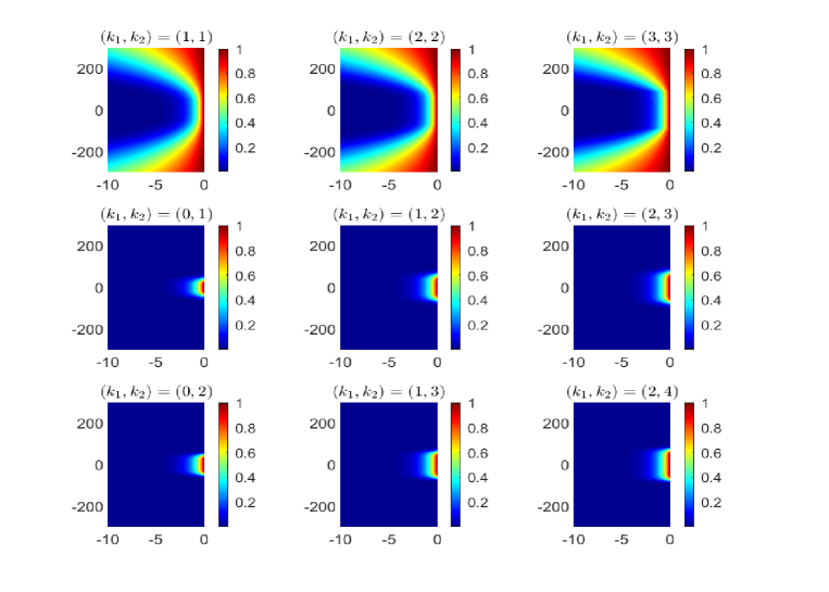
Fig. 3: Stability domain of the block generalized Adams method with $0\leq k_{2}-k_{1}\leq 2.$

Suppose the block generalized Adams method is $A(\theta)-$stable with $\theta>\phi$ and Assumption 2.1 is satisfied. For any complex number $z$ locating in the domain $\mathbb{C}\setminus\mathbb{C}_{\varphi}$ and $|\zeta|<1,$ it follows that

$$\Delta(\zeta)-z\mathbf{E}_{m}= (\mathbf{A}+\zeta\mathbf{D})^{-1}((\mathbf{B}-\zeta\mathbf{C})-z(\mathbf{A}+\zeta\mathbf{D}))$$

$$= (\mathbf{A}+\zeta\mathbf{D})^{-1}((\mathbf{B}-z\mathbf{A})-\zeta(\mathbf{C}+z\mathbf{D}))$$

Since all eigenvalues of $\mathbf{A}^{-1}\mathbf{B}$ locate at the domain $\mathbb{C}_{\varphi},$ we obtain $\mathbf{B}-z\mathbf{A}$ is invertible according to Assumption 2.1. Therefore, we have

$$\Delta(\zeta)-z\mathbf{E}_{m}=(\mathbf{A}+\zeta\mathbf{D})^{-1}(\mathbf{B}-z\mathbf{A})(\mathbf{E}_{m}-\zeta(\mathbf{B}-z\mathbf{A})^{-1}(\mathbf{C}+z\mathbf{D})).$$

Noting that for $j\geq 2$

$$((\mathbf{B}-z\mathbf{A})^{-1}(\mathbf{C}+z\mathbf{D}))^{j}= ((\mathbf{B}-z\mathbf{A})^{-1}(\mathbf{C}+z\mathbf{D})\mathbf{e}_{m}\mathbf{e}^{T}_{m})^{j}$$

$$= \mathbf{R}^{j-1}(z)(\mathbf{B}-z\mathbf{A})^{-1}(\mathbf{C}+z\mathbf{D})$$

and $|\mathbf{R}^{j-1}(z)|\leq 1,$ we obtain $\mathbf{E}_{m}-\zeta(\mathbf{B}-z\mathbf{A})^{-1}(\mathbf{C}+z\mathbf{D})$ is invertible with $|\zeta|<1.$ Finally, we conclude that all eigenvalues of $\Delta(\zeta)$ lie in the domain $\mathbb{C}_{\varphi}.$ According to Cauchy’s integral formula, we have

(30) $$\mathbf{U}(\zeta)=\frac{1}{2\pi\mathrm{i}}\int_{\Gamma}K(\lambda)\left(\Delta(\zeta)/h-\lambda\mathbf{E}_{m}\right)^{-1}\mathbf{G}(\zeta)d\lambda=K\left(\Delta(\zeta)/h\right)\mathbf{G}(\zeta),$$

where $\mathbf{U}(\zeta)=\sum_{n=0}^{\infty}\mathbf{U}_{n}\zeta^{n},$ $\mathbf{U}_{n}=(u^{n}_{1}~{}~{}\cdots~{}~{}u^{n}_{m})^{T}$ and $u^{n}_{j}$ denotes the approximation to $\mathrm{I}[k,g](t^{n}_{j}).$ Then BGACQ${}_{k_{1},k_{2}}$ is defined by

(31) $$\mathbf{U}_{n}=\sum_{j=0}^{n}\mathbf{W}_{j}\mathbf{G}_{n-j},~{}~{}n=0,1,\cdots,N,$$

where $K\left(\Delta(\zeta)/h\right)=\sum_{n=0}^{\infty}\mathbf{W}_{n}\zeta^{n}.$ Particularly, we obtain approximations to CI (1) at $t^{n+1}\in\mathbb{X}_{N}$ by

(32) $$\mathrm{I}[k,g](t^{n+1})\approx\mathbf{e}_{m}^{T}\sum_{j=0}^{n}\mathbf{W}_{j}\mathbf{G}_{n-j}.$$

In this paper, we use the composite trapezoid rule to numerically compute the coefficient matrix $\mathbf{W}_{j},$ that is,

$$\mathbf{W}_{j}=\frac{1}{2\pi\mathrm{i}}\int_{|\zeta|=\rho}K\left(\Delta(\zeta)/h\right)\zeta^{-j-1}d\zeta\approx\frac{\rho^{-j}}{L}\sum_{l=0}^{L-1}K\left(\Delta\left(\rho\mathrm{e}^{\mathrm{i}l2\pi/L}\right)/h\right)\mathrm{e}^{-\mathrm{i}jl2\pi/L},$$

where $\rho=\mathrm{tol}^{1/L},$ $L=10Nm$ and $\mathrm{tol}=10^{-16}.$

The above BGACQ${}_{k_{1},k_{2}}$ can be seemed to be a special class of multistage CQs. It has a similar structure to RKCQ and also uses a two-grid method. However, BGACQ${}_{k_{1},k_{2}}$ allows us to easily change the size of the matrix in the discrete differentiation symbol by selecting the parameter $m.$ Meanwhile, it is possible to construct many high-order stable algorithms by choosing the parameters $k_{1},k_{2},m.$

3 Analysis for BGACQ${}_{k_{1},k_{2}}$

In this section, we investigate the convergence property of BGACQ${}_{k_{1},k_{2}}$ when the stepsize $h$ of the coarse grid $\mathbb{X}_{N}$ is reduced and the parameters $k_{1},k_{2},m$ are fixed. Following the work of [18], we firstly explore the numerical error of the block generalized Adams method for IVP (6). Then the error bound for BGACQ${}_{k_{1},k_{2}}$ is analyzed by integrating the product of the numerical error and $K(\lambda)$ over the curve $\Gamma.$ The convergence property of BGACQ${}_{k_{1},k_{2}}$ with respect to the stepsize $h$ is summarized in the following theorem.

Theorem 1.

Suppose that

• The Laplace transform $K$ of the kernel function $k$ is analytic in the sector $\mathbb{C}_{\varphi};$

• $g$ has a continuous derivative of order $k_{1}+k_{2}+2$ over $[0,T];$

• Assumption 2.1 is satisfied.

Then, for any $n$ satisfying $0\leq n\leq N-1,$ the difference between $\mathrm{I}[k,g](t^{n+1})$ and $u^{n}_{m}$ computed by BGACQ${}_{k_{1},k_{2}}$ satisfies

$$|\mathrm{I}[k,g](t^{n+1})-u^{n}_{m}|\leq Ch^{k_{1}+k_{2}+2}(\sum_{l=1}^{k_{1}+k_{2}+1}g^{(l)}(0)(1+(nh)^{\mu+l-k_{1}-k_{2}-2})+h^{\mu}+1).$$

where the constant $C$ is independent of $h.$

Proof.

We begin by exploring the interpolation remainder in three cases as is done in Section 2. In the case of $t\in[t^{n}_{0},t^{n}_{k_{1}}],$ we can represent the remainder $f(t)-f_{N}(t)$ by Peano’s kernel theorem [7, pp. 43] in the form of

$$f(t^{n}_{k_{1}}+sh/m)-f_{N}(t^{n}_{k_{1}}+sh/m)=h^{k_{1}+k_{2}+2}\mathcal{E}_{k_{1}}(s),$$

where $\mathcal{E}_{k_{1}}(s)=\int_{-k_{1}}^{k_{2}+1}\kappa(s,v)f^{(k_{1}+k_{2}+2)}(t^{n}_{k_{1}}+vh/m)dv$ with $s\in[-k_{1},0],$ and the kernel $\kappa(s,v)$ is defined by

$$\kappa(s,v)=\frac{1}{(k_{1}+k_{2}+1)!}\left((s-v)_{+}^{k_{1}+k_{2}+1}-\sum_{i=-k_{1}}^{k_{2}+1}\phi_{i}^{k_{1},k_{2}}(s)(i-v)_{+}^{k_{1}+k_{2}+1}\right).$$

If $t\in[t^{n}_{j},t^{n}_{j+1}]$ with $j=k_{1},\cdots,m-k_{2}-1,$ we can represent $f(t)-f_{N}(t)$ by

$$f(t^{n}_{j}+sh/m)-f_{N}(t^{n}_{j}+sh/m)=h^{k_{1}+k_{2}+2}\mathcal{E}_{j}(s),$$

where $\mathcal{E}_{j}(s)=\int_{-k_{1}}^{k_{2}+1}\kappa(s,v)f^{(k_{1}+k_{2}+2)}(t^{n}_{j}+vh/m)dv$ with $s\in[0,1],$ and the kernel is defined as the same as above. In the case of $t\in[t^{n}_{j},t^{n}_{j+1}]$ with $j=m-k_{2},\cdots,m-1,$ the approximation error is represented by

$$f(t^{n}_{m-k_{2}-1}+sh/m)-f_{N}(t^{n}_{m-k_{2}-1}+sh/m)=h^{k_{1}+k_{2}+2}\mathcal{E}_{m-k_{2}-1}(s),$$

where $\mathcal{E}_{m-k_{2}-1}(s)=\int_{-k_{1}}^{k_{2}+1}\kappa(s,v)f^{(k_{1}+k_{2}+2)}(t^{n}_{m-k_{2}-1}+vh/m)dv$ with $s\in[1,k_{2}+1].$ As a result, the quadrature error $q^{n}_{j+1}$ produced by the quadrature rule (24) is represented by

$$q^{n}_{j+1}=\left\{\begin{array}[]{l}\frac{h^{k_{1}+k_{2}+3}}{m}\int_{j-k_{1}}^{j-k_{1}+1}\mathcal{E}_{k_{1}}(s)ds,~{}~{}j=0,\cdots,k_{1}-1,\\ \frac{h^{k_{1}+k_{2}+3}}{m}\int_{0}^{1}\mathcal{E}_{j}(s)ds,~{}~{}j=k_{1},\cdots,m-k_{2}-1,\\ \frac{h^{k_{1}+k_{2}+3}}{m}\int_{j-m+k_{2}+1}^{j-m+k_{2}+2}\mathcal{E}_{m-k_{2}-1}(s)ds,~{}~{}j=m-k_{2},\cdots,m-1.\end{array}\right.$$

For $n=0,\cdots,N-1,$ defining $\mathbf{Q}_{n}=\left(\begin{array}[]{cccc}q^{n}_{1}&q^{n}_{2}&\cdots&q^{n}_{m}\\ \end{array}\right),$ we have

(33) $$\mathbf{B}\mathbf{Y}_{n}^{ref}-\mathbf{C}\mathbf{Y}_{n-1}^{ref}=h\lambda\mathbf{D}\mathbf{Y}_{n-1}^{ref}+h\lambda\mathbf{A}\mathbf{Y}_{n}^{ref}+h\mathbf{D}\mathbf{G}_{n-1}+h\mathbf{A}\mathbf{G}_{n}+\mathbf{Q}_{n}.$$

According to Eqs. (25) and (33), we obtain by a direct calculation

(34) $$\mathbf{B}(\mathbf{Y}_{n}^{ref}-\mathbf{Y}_{n})-\mathbf{C}(\mathbf{Y}_{n-1}^{ref}-\mathbf{Y}_{n-1})=h\lambda\mathbf{D}(\mathbf{Y}_{n-1}^{ref}-\mathbf{Y}_{n-1})+h\lambda\mathbf{A}(\mathbf{Y}_{n}^{ref}-\mathbf{Y}_{n})+\mathbf{Q}_{n}.$$

Denoting the collocation error $\epsilon^{n}=y(t^{n}_{m})-y^{n}_{m}$ and $\epsilon^{-1}=0,$ we get

(35) $$\epsilon^{n}=\mathbf{R}(h\lambda)\epsilon^{n-1}+\mathbf{e}_{m}^{T}(\mathbf{B}-h\lambda\mathbf{A})^{-1}\mathbf{Q}_{n}.$$

As a result, we have

(36) $$\epsilon^{n}=\sum_{j=0}^{n}\mathbf{R}^{j}(h\lambda)\mathbf{e}_{m}^{T}(\mathbf{B}-h\lambda\mathbf{A})^{-1}\mathbf{Q}_{n-j}.$$

Now let us turn to consider the bound for $\left|\int_{\Gamma}K(\lambda)\epsilon^{n}d\lambda\right|.$ First of all, we split the curve $\Gamma$ into three parts, that is,

$$\Gamma_{1}:= \{\lambda:\lambda\in\Gamma,|\lambda|\leq\textsc{Const}\},$$

$$\Gamma_{2}:= \{\lambda:\lambda\in\Gamma,h\textsc{Const}\leq|h\lambda|\leq 1,\mathrm{arg}(\lambda)=\pi-\varphi\},$$

$$\Gamma_{3}:= \{\lambda:\lambda\in\Gamma,|h\lambda|\geq 1,\mathrm{arg}(\lambda)=\pi-\varphi\},$$

where Const is a given positive number.

Assumption 2.1 states that there exists a constant $h_{0}$ such that for any $h\in(0,h_{0}),$ the maximum norm of the inverse of $\mathbf{B}-h\lambda\mathbf{A}$ is bounded by a constant $M_{AB}$ that is independent of $h$ and $\lambda$ for any $\lambda\in\Gamma_{1}.$ Hence, we obtain

$$\|\mathbf{e}_{m}^{T}(\mathbf{B}-h\lambda\mathbf{A})^{-1}\mathbf{1}\|\leq M_{AB},~{}~{}\lambda\in\Gamma_{1},$$

where $\|\cdot\|$ denotes the maximum norm, $\mathbf{1}$ denotes the $m\times 1$ vector with all elements being $1.$ Besides, since $\mathbf{R}(h\lambda)$ is an approximation to $\mathrm{e}^{h\lambda},$ $|\mathbf{R}^{n}(h\lambda)|$ is bounded by a constant $M_{R}.$ On the other hand, noting that

$$\lambda y^{(k_{1}+k_{2}+2)}(t)=\sum_{l=0}^{k_{1}+k_{2}+1}\lambda^{k_{1}+k_{2}+2-l}\mathrm{e}^{\lambda t}g^{(l)}(0)+\lambda\int_{0}^{t}g^{(k_{1}+k_{2}+2)}(t-s)\mathrm{e}^{\lambda s}ds,$$

we show that $\|\mathbf{Q}_{n}\|$ is of order $1$ as the stepsize $h$ reduces when $\lambda$ falls in the curve $\Gamma_{1}.$ Letting

$$M_{\kappa}:=\max_{s\in[-k_{1},k_{2}+1]}\left\{\int_{-k_{1}}^{k_{2}+1}|\kappa(s,v)|dv\right\},~{}~{}M_{f}^{1}:=\max_{t\in[0,T],\lambda\in\Gamma_{1}}\{|f^{(k_{1}+k_{2}+2)}(t)|\},$$

we obtain for $n=0,1,\cdots,N-1,$

(37) $$\|\mathbf{Q}_{n}\|\leq\frac{h^{k_{1}+k_{2}+3}}{m}M_{\kappa}M_{f}^{1}.$$

As a result, we have

$$\left|\int_{\Gamma_{1}}K(\lambda)\epsilon^{n}d\lambda\right|\leq \frac{M_{AB}M_{\kappa}M_{f}^{1}}{m}h^{k_{1}+k_{2}+3}\int_{\Gamma_{1}}|K(\lambda)|\left(\sum_{j=0}^{n}|\mathbf{R}^{j}(h\lambda)|\right)|d\lambda|$$

$$\leq \frac{M_{AB}M_{\kappa}M_{f}^{1}M_{R}T}{m}\int_{\Gamma_{1}}|K(\lambda)||d\lambda|h^{k_{1}+k_{2}+2}=C_{1}h^{k_{1}+k_{2}+2},$$

where $C_{1}=\frac{M_{AB}M_{\kappa}M_{f}^{1}M_{R}T}{m}\int_{\Gamma_{1}}|K(\lambda)||d\lambda|.$

In the case of $\lambda\in\Gamma_{2},$ we suppose $|\mathbf{R}(h\lambda)|$ is bounded by $C_{R}<1.$ It follows that

$$\left|\int_{\Gamma_{2}}K(\lambda)\epsilon^{n}d\lambda\right|$$

$$\leq \frac{M_{\kappa}M_{AB}}{m}\sum_{l=1}^{k_{1}+k_{2}+1}g^{(l)}(0)h^{k_{1}+k_{2}+3}\int_{\Gamma_{2}}|K(\lambda)|\sum_{j=0}^{n}|\mathbf{R}^{j}(h\lambda)||\lambda|^{k_{1}+k_{2}+2-l}|\mathrm{e}^{\lambda t^{n}}||d\lambda|$$

$$+\frac{M_{\kappa}M_{AB}M_{g}^{n}}{m}h^{k_{1}+k_{2}+3}\int_{\Gamma_{2}}|K(\lambda)|\sum_{j=0}^{n}|\mathbf{R}^{j}(h\lambda)||\mathrm{e}^{\lambda t^{n}}||d\lambda|,$$

where $M_{g}^{n}:=\max_{0\leq t\leq t^{n}}\{g^{(k_{1}+k_{2}+2)}(t)\}.$ Noting that

$$\sum_{j=0}^{n}|\mathbf{R}^{j}(h\lambda)|=\frac{1-|\mathbf{R}^{n}(h\lambda)|}{1-|\mathbf{R}(h\lambda)|}\leq\frac{1}{1-C_{R}},$$

we have

$$\left|\int_{\Gamma_{2}}K(\lambda)\epsilon^{n}d\lambda\right|$$

$$\leq \frac{M_{\kappa}M_{AB}M}{m(1-C_{R})}\sum_{l=1}^{k_{1}+k_{2}+1}g^{(l)}(0)\int_{\Gamma_{2}}|\lambda|^{-\mu-l-1}|h\lambda|^{k_{1}+k_{2}+2}|\mathrm{e}^{\lambda t^{n}}||d\lambda|$$

$$+\frac{M_{\kappa}M_{AB}M_{g}^{n}M}{m(1-C_{R})}h^{k_{1}+k_{2}+2}\int_{\Gamma_{2}}|\lambda|^{-\mu-1}|h\lambda||\mathrm{e}^{\lambda t^{n}}||d\lambda|.$$

In addition, there exist constants $C_{\lambda}^{1}$ and $C_{\lambda}^{2}$ independent of $h$ such that

$$\int_{\Gamma_{2}}|\lambda|^{-\mu-l-1}|h\lambda|^{k_{1}+k_{2}+2}|\mathrm{e}^{\lambda t^{n}}||d\lambda|\leq C_{\lambda}^{1}h^{k_{1}+k_{2}+2}(1+(nh)^{\mu+l-k_{1}-k_{2}-2})$$

and

$$\int_{\Gamma_{2}}|\lambda|^{-\mu-1}||h\lambda||\mathrm{e}^{\lambda t^{n}}||d\lambda|\leq C_{\lambda}^{2}h(1+(nh)^{\mu-1}).$$

Hence, we obtain

$$\left|\int_{\Gamma_{2}}K(\lambda)\epsilon^{n}d\lambda\right|$$

$$\leq \frac{M_{\kappa}M_{AB}MC_{\lambda}^{1}}{m(1-C_{R})}\sum_{l=1}^{k_{1}+k_{2}+1}g^{(l)}(0)h^{k_{1}+k_{2}+2}(1+(nh)^{\mu+l-k_{1}-k_{2}-2})$$

$$+\frac{M_{\kappa}M_{AB}M_{g}^{n}MC_{\lambda}^{2}}{m(1-C_{R})}h^{k_{1}+k_{2}+3}(1+(nh)^{\mu-1})$$

$$= C_{2}\sum_{l=1}^{k_{1}+k_{2}+1}g^{(l)}(0)h^{k_{1}+k_{2}+2}(1+(nh)^{\mu+l-k_{1}-k_{2}-2})+C_{3}h^{k_{1}+k_{2}+3}(1+(nh)^{\mu-1}),$$

where $C_{2}=\frac{M_{\kappa}M_{AB}MC_{\lambda}^{1}}{m(1-C_{R})}$ and $C_{3}=\frac{M_{\kappa}M_{AB}M_{g}^{n}MC_{\lambda}^{2}}{m(1-C_{R})}.$

In the case of $\lambda\in\Gamma_{3},$ it can be shown that $f^{(k_{1}+k_{2}+2)}(t)$ is bounded by a constant $M_{f}^{3}$. Besides, Assumption 2.1 indicates that $\|(\mathbf{B}-h\lambda\mathbf{A})^{-1}\||h\lambda|$ is bounded by a constant $\hat{M}_{AB}.$ As a result, we get

$$\left|\int_{\Gamma_{3}}K(\lambda)\epsilon^{n}d\lambda\right|\leq \frac{h^{k_{1}+k_{2}+2}M_{\kappa}M_{f}^{3}}{m}\int_{\Gamma_{3}}|K(\lambda)|\sum_{j=0}^{n}|\mathbf{R}(h\lambda)|^{j}|h\lambda|^{-1}\|(\mathbf{B}-h\lambda\mathbf{A})^{-1}\||h\lambda||d\lambda|$$

$$\leq \frac{MM_{\kappa}M_{f}^{3}\hat{M}_{AB}}{m(1-C_{R})}\int_{\Gamma_{3}}|\lambda|^{-\mu-1}|d\lambda|h^{k_{1}+k_{2}+2}=C_{4}h^{k_{1}+k_{2}+2},$$

where $C_{4}=\frac{MM_{\kappa}M_{f}^{3}\hat{M}_{AB}}{m(1-C_{R})}\int_{\Gamma_{3}}|\lambda|^{-\mu-1}|d\lambda|.$

Letting $C=\max\{3C_{1},C_{2},3C_{3},3C_{4}\},$ we arrive at the estimation

$$|\mathrm{I}[k,g](t^{n+1})-u^{n}_{m}|\leq Ch^{k_{1}+k_{2}+2}(\sum_{l=1}^{k_{1}+k_{2}+1}g^{(l)}(0)(1+(nh)^{\mu+l-k_{1}-k_{2}-2})+h^{\mu}+1).$$

This completes the proof. ∎

Removing the assumption $g(0)=0$ from the previous theorem will introduce an error term in Eq. (25), which definitely has a negative impact on the convergence rate of BGACQ${}_{k_{1},k_{2}}.$ Meanwhile, the pointwise error at $t^{1}$ depends heavily on the derivatives of $g(t)$ at $t=0.$ Therefore, we should modify BGACQ${}_{k_{1},k_{2}}$ by firstly solving the following equations for $i=1,\cdots,m,$ and $q=0,1,\cdots,k_{1}+k_{2}+1,$

(38) $$\mathrm{I}[k,t^{q}](t^{n}_{i})=\mathbf{e}_{i}^{T}\sum_{j=0}^{n}\mathbf{W}_{n-j}\mathbf{t}^{j}_{q}+\sum_{j=0}^{k_{1}+k_{2}+1}\omega_{i,j}^{n}(t_{j}^{0})^{q},$$

where $\mathbf{e}_{i}$ denotes the $m\times 1$ column vector with all elements being zero except for the $i$-th element, which is one, and $\mathbf{t}^{j}_{q}=((t_{1}^{j})^{q}~{}~{}(t_{2}^{j})^{q}~{}~{}\cdots~{}~{}(t_{m}^{j})^{q})^{T}.$ Then, the modified BGACQ${}_{k_{1},k_{2}}$ (MBGACQ${}_{k_{1},k_{2}}$) is defined by

(39) $$\mathrm{I}[k,g](t^{n+1})\approx\mathbf{e}_{m}^{T}\sum_{j=0}^{n}\mathbf{W}_{n-j}\mathbf{G}_{j}+\sum_{j=0}^{k_{1}+k_{2}+1}\omega_{m,j}^{n}g(t_{j}^{0}).$$

By checking the convergence results in Theorem 1, it can be easily founded that MBGACQ${}_{k_{1},k_{2}}$ has a uniform convergence order of $k_{1}+k_{2}+2$ on the interval $[0,T].$

According to Theorem 1, the stability function $\mathbf{R}(z)$ approximates $\mathrm{e}^{z}$ with a convergence order of $\mathcal{O}(z^{k_{1}+k_{2}+2})$ as $z$ approaches zero. In Tables 2 and 3 , we compute Taylor’s expansion of $\mathbf{R}(z)-\mathrm{e}^{z}$ for BGACQ${}_{k_{1},k_{2}}$ with various $k_{1},k_{2},m.$ As a comparison, the same expansions for RKCQs are listed in Table 4. We find that the dissipation of BGACQ${}_{k_{1},k_{2}}$ can be improved by increasing the stage parameter $m.$ The dissipation of RKCQ, on the other hand, is fixed. Therefore, BGACQ${}_{k_{1},k_{2}}$ is expected to have a great potential for solving long-time integration problems with a good stability.

Table 2: Expansion of the stability function of BGACQ${}_{k_{1},k_{2}}$ with $m=10.$

  $(k_{1},k_{2})=(1,0)$ $\mathrm{e}^{z}+3.3\times 10^{-5}z^{4}+3.2\times 10^{-5}z^{5}+\mathcal{O}(z^{6})$ $(k_{1},k_{2})=(1,2)$ $\mathrm{e}^{z}+4.6\times 10^{-8}z^{6}+4.3\times 10^{-8}z^{7}+\mathcal{O}(z^{8})$ $(k_{1},k_{2})=(1,3)$ $\mathrm{e}^{z}+3.3\times 10^{-11}z^{7}-1.7\times 10^{-10}z^{8}+\mathcal{O}(z^{9})$ $(k_{1},k_{2})=(1,4)$ $\mathrm{e}^{z}+1.2\times 10^{-10}z^{8}+8.2\times 10^{-11}z^{9}+\mathcal{O}(z^{10})$  

Table 3: Expansion of the stability function of BGACQ${}_{k_{1},k_{2}}$ with $m=50.$

  $(k_{1},k_{2})=(1,0)$ $\mathrm{e}^{z}+3.2\times 10^{-7}z^{4}+3.2\times 10^{-7}z^{5}+\mathcal{O}(z^{6})$ $(k_{1},k_{2})=(1,2)$ $\mathrm{e}^{z}+2.3\times 10^{-11}z^{6}+2.2\times 10^{-11}z^{7}+\mathcal{O}(z^{8})$ $(k_{1},k_{2})=(1,3)$ $\mathrm{e}^{z}-2.3\times 10^{-13}z^{7}-2.3\times 10^{-13}z^{8}+\mathcal{O}(z^{9})$ $(k_{1},k_{2})=(1,4)$ $\mathrm{e}^{z}+3.3\times 10^{-15}z^{8}+3.3\times 10^{-15}z^{9}+\mathcal{O}(z^{10})$  

Table 4: Expansion of the stability function of RKCQs.

  2-stage Radau IIA $\mathrm{e}^{z}-1.4\times 10^{-2}z^{4}-1.8\times 10^{-2}z^{5}+\mathcal{O}(z^{6})$ 3-stage Radau IIA $\mathrm{e}^{z}+1.4\times 10^{-4}z^{6}+1.6\times 10^{-4}z^{7}+\mathcal{O}(z^{8})$ 3-stage Lobatto IIIC $\mathrm{e}^{z}+2.1\times 10^{-3}z^{5}+2.9\times 10^{-3}z^{6}+\mathcal{O}(z^{7})$ 4-stage Lobatto IIIC $\mathrm{e}^{z}-1.3\times 10^{-5}z^{7}-1.7\times 10^{-5}z^{8}+\mathcal{O}(z^{9})$  

4 Numerical Experiments

In this section, we first give several numerical experiments that confirm the theoretical estimation in Theorem 1. In addition, we consider the application of MBGACQ${}_{k_{1},k_{2}}$ to numerical solutions to integral equations with weakly singular kernels and rapidly varying solutions.

4.1 CI with a Smooth Kernel

We first test the performance of BGACQ${}_{k_{1},k_{2}}$ by numerically solving the following CI

(40) $$\int_{0}^{t}\mathrm{e}^{-(t-s)}\cos(s)ds,~{}~{}t\in[0,10].$$

The Laplace transform of $\mathrm{e}^{-t}$ is $1/(\lambda+1),$ which is analytic in the whole complex plane except for $\lambda=-1$. In Tables 5–6, we show the magnitude of the quadrature error at $t=10$ denoted as ‘$\mathrm{Err}_{N}$’ with various $N.$ The stage parameter $m$ is fixed to be $8.$ Besides, we compute in these tables the numerical rates of quadrature errors by

$$\mathrm{Order}=\log_{2}\left(\frac{\mathrm{Err}_{N_{1}}}{\mathrm{Err}_{N_{2}}}\right)/\log_{2}\left(\frac{N_{2}}{N_{1}}\right).$$

The expected convergence order of BGACQ${}_{k_{1},k_{2}}$ is $1,$ since $\cos(s)$ does not vanish at $s=0.$ It can be seen from Table 5 the numerical results match this estimation. In Table 6, it is found that the computed convergence order of MBGACQ${}_{k_{1},k_{2}}$ is approximately $k_{1}+k_{2}+2,$ which coincides well with the theoretical estimation in Theorem 1. In Table 7, we show the pointwise errors and convergence orders of MBGACQ${}_{k_{1},k_{2}}$ at $t^{1}.$ The rapid decrease in quadrature errors with increasing $N$ in this table suggests that MBGACQ${}_{k_{1},k_{2}}$ is uniformly convergent.

Table 5: Errors and convergence rates of BGACQ${}_{k_{1},k_{2}}$ for CI (40) with $m=8$ at $t=10.$

  $N$ $(k_{1},k_{2})=(1,1)$ $(k_{1},k_{2})=(1,2)$ $(k_{1},k_{2})=(1,3)$ $\mathrm{Err}_{N}$ $\mathrm{Order}$ $\mathrm{Err}_{N}$ $\mathrm{Order}$ $\mathrm{Err}_{N}$ $\mathrm{Order}$ 8 $1.14\times 10^{-6}$ - $2.18\times 10^{-6}$ - $2.27\times 10^{-6}$ - 10 $1.41\times 10^{-6}$ -0.9 $1.82\times 10^{-6}$ 0.8 $1.81\times 10^{-6}$ 1.0 12 $1.36\times 10^{-6}$ 0.2 $1.54\times 10^{-6}$ 0.9 $1.51\times 10^{-6}$ 1.0 14 $1.24\times 10^{-6}$ 0.6 $1.32\times 10^{-6}$ 1.0 $1.29\times 10^{-6}$ 1.0 16 $1.12\times 10^{-6}$ 0.8 $1.16\times 10^{-6}$ 1.0 $1.12\times 10^{-6}$ 1.0  

Table 6: Errors and convergence rates of MBGACQ${}_{k_{1},k_{2}}$ for CI (40) with $m=8$ at $t=10.$

  $N$ $(k_{1},k_{2})=(1,1)$ $(k_{1},k_{2})=(1,2)$ $(k_{1},k_{2})=(1,3)$ $\mathrm{Err}_{N}$ $\mathrm{Order}$ $\mathrm{Err}_{N}$ $\mathrm{Order}$ $\mathrm{Err}_{N}$ $\mathrm{Order}$ 8 $1.28\times 10^{-6}$ - $1.83\times 10^{-7}$ - $1.04\times 10^{-8}$ - 10 $5.18\times 10^{-7}$ 4.1 $5.51\times 10^{-8}$ 5.4 $2.46\times 10^{-9}$ 6.5 12 $2.47\times 10^{-7}$ 4.1 $2.07\times 10^{-8}$ 5.4 $7.72\times 10^{-10}$ 6.4 14 $1.33\times 10^{-7}$ 4.0 $9.11\times 10^{-9}$ 5.3 $2.94\times 10^{-10}$ 6.3 16 $7.73\times 10^{-8}$ 4.0 $4.48\times 10^{-9}$ 5.3 $1.28\times 10^{-10}$ 6.2  

Table 7: Errors and convergence rates of MBGACQ${}_{k_{1},k_{2}}$ for CI (40) with $m=8$ at $t^{1}.$

  $N$ $(k_{1},k_{2})=(1,1)$ $(k_{1},k_{2})=(1,2)$ $(k_{1},k_{2})=(1,3)$ $\mathrm{Err}_{N}$ $\mathrm{Order}$ $\mathrm{Err}_{N}$ $\mathrm{Order}$ $\mathrm{Err}_{N}$ $\mathrm{Order}$ 8 $1.20\times 10^{-6}$ - $1.96\times 10^{-7}$ - $6.39\times 10^{-9}$ - 10 $4.90\times 10^{-7}$ 4.0 $4.94\times 10^{-8}$ 6.2 $2.01\times 10^{-9}$ 5.2 12 $2.29\times 10^{-7}$ 4.2 $1.54\times 10^{-8}$ 6.4 $6.82\times 10^{-10}$ 5.9 14 $1.18\times 10^{-7}$ 4.3 $5.66\times 10^{-9}$ 6.5 $2.61\times 10^{-10}$ 6.2 16 $6.57\times 10^{-8}$ 4.4 $2.35\times 10^{-9}$ 6.6 $1.11\times 10^{-10}$ 6.4  

4.2 CI with a Weakly Singular Kernel

Next, we consider the application of MBGACQ${}_{k_{1},k_{2}}$ to the calculation of the fractional integral

(41) $$\frac{1}{\Gamma(\alpha)}\int_{0}^{t}(t-s)^{\alpha-1}(\sin(s)+1)\mathrm{e}^{0.8s}ds,~{}~{}t\in[0,10],$$

where $\alpha\in(0,1).$ The computed errors at $t=10$ are listed in Tables 8–10, where we can see the parameter $\alpha$ does not affect the convergence rate of MBGACQ${}_{k_{1},k_{2}}.$ In Tables 11–13, we again list the computed errors at $t^{1},$ which indicates the convergence of MBGACQ${}_{k_{1},k_{2}}$ is uniform.

Table 8: Errors and convergence rates of MBGACQ${}_{k_{1},k_{2}}$ for CI (41) with $\alpha=0.1,~{}m=16$ at $t=10.$

  $N$ $(k_{1},k_{2})=(1,1)$ $(k_{1},k_{2})=(1,2)$ $(k_{1},k_{2})=(1,3)$ $\mathrm{Err}_{N}$ $\mathrm{Order}$ $\mathrm{Err}_{N}$ $\mathrm{Order}$ $\mathrm{Err}_{N}$ $\mathrm{Order}$ 8 $5.87\times 10^{-5}$ - $2.50\times 10^{-5}$ - $5.19\times 10^{-7}$ - 10 $4.25\times 10^{-5}$ 1.5 $7.76\times 10^{-6}$ 5.2 $1.31\times 10^{-7}$ 6.1 12 $2.65\times 10^{-5}$ 2.6 $3.00\times 10^{-6}$ 5.2 $4.21\times 10^{-8}$ 6.3 14 $1.66\times 10^{-5}$ 3.0 $1.35\times 10^{-6}$ 5.2 $1.59\times 10^{-8}$ 6.3 16 $1.08\times 10^{-5}$ 3.3 $6.77\times 10^{-7}$ 5.2 $6.91\times 10^{-9}$ 6.2  

Table 9: Errors and convergence rates of MBGACQ${}_{k_{1},k_{2}}$ for CI (41) with $\alpha=0.5,~{}m=16$ at $t=10.$

  $N$ $(k_{1},k_{2})=(1,1)$ $(k_{1},k_{2})=(1,2)$ $(k_{1},k_{2})=(1,3)$ $\mathrm{Err}_{N}$ $\mathrm{Order}$ $\mathrm{Err}_{N}$ $\mathrm{Order}$ $\mathrm{Err}_{N}$ $\mathrm{Order}$ 8 $5.77\times 10^{-4}$ - $1.04\times 10^{-4}$ - $2.11\times 10^{-6}$ - 10 $2.80\times 10^{-4}$ 3.2 $3.29\times 10^{-5}$ 5.2 $5.38\times 10^{-7}$ 6.1 12 $1.48\times 10^{-4}$ 3.5 $1.29\times 10^{-5}$ 5.1 $1.76\times 10^{-7}$ 6.1 14 $8.47\times 10^{-5}$ 3.6 $5.86\times 10^{-6}$ 5.1 $6.80\times 10^{-8}$ 6.2 16 $5.16\times 10^{-5}$ 3.7 $2.96\times 10^{-6}$ 5.1 $3.04\times 10^{-8}$ 6.0  

Table 10: Errors and convergence rates of MBGACQ${}_{k_{1},k_{2}}$ for CI (41) with $\alpha=0.9,~{}m=16$ at $t=10.$

  $N$ $(k_{1},k_{2})=(1,1)$ $(k_{1},k_{2})=(1,2)$ $(k_{1},k_{2})=(1,3)$ $\mathrm{Err}_{N}$ $\mathrm{Order}$ $\mathrm{Err}_{N}$ $\mathrm{Order}$ $\mathrm{Err}_{N}$ $\mathrm{Order}$ 8 $7.34\times 10^{-4}$ - $1.53\times 10^{-4}$ - $3.84\times 10^{-6}$ - 10 $3.32\times 10^{-4}$ 3.6 $4.86\times 10^{-5}$ 5.1 $9.87\times 10^{-7}$ 6.1 12 $1.69\times 10^{-4}$ 3.7 $1.91\times 10^{-5}$ 5.1 $3.26\times 10^{-7}$ 6.1 14 $9.38\times 10^{-5}$ 3.8 $8.70\times 10^{-6}$ 5.1 $1.29\times 10^{-7}$ 6.0 16 $5.61\times 10^{-5}$ 3.9 $4.41\times 10^{-6}$ 5.1 $5.79\times 10^{-8}$ 6.0  

Table 11: Errors and convergence rates of MBGACQ${}_{k_{1},k_{2}}$ for CI (41) with $\alpha=0.1,~{}m=16$ at $t^{1}.$

  $N$ $(k_{1},k_{2})=(1,1)$ $(k_{1},k_{2})=(1,2)$ $(k_{1},k_{2})=(1,3)$ $\mathrm{Err}_{N}$ $\mathrm{Order}$ $\mathrm{Err}_{N}$ $\mathrm{Order}$ $\mathrm{Err}_{N}$ $\mathrm{Order}$ 8 $1.42\times 10^{-7}$ - $8.07\times 10^{-9}$ - $7.54\times 10^{-10}$ - 10 $4.56\times 10^{-8}$ 5.1 $3.29\times 10^{-9}$ 4.0 $1.26\times 10^{-10}$ 8.0 12 $1.87\times 10^{-8}$ 4.9 $1.35\times 10^{-9}$ 4.9 $3.08\times 10^{-11}$ 7.7 14 $8.98\times 10^{-9}$ 4.8 $6.09\times 10^{-10}$ 5.2 $9.68\times 10^{-12}$ 7.5 16 $4.80\times 10^{-9}$ 4.7 $3.01\times 10^{-10}$ 5.3 $3.66\times 10^{-12}$ 7.3  

Table 12: Errors and convergence rates of MBGACQ${}_{k_{1},k_{2}}$ for CI (41) with $\alpha=0.5,~{}m=16$ at $t^{1}.$

  $N$ $(k_{1},k_{2})=(1,1)$ $(k_{1},k_{2})=(1,2)$ $(k_{1},k_{2})=(1,3)$ $\mathrm{Err}_{N}$ $\mathrm{Order}$ $\mathrm{Err}_{N}$ $\mathrm{Order}$ $\mathrm{Err}_{N}$ $\mathrm{Order}$ 8 $8.57\times 10^{-7}$ - $5.18\times 10^{-8}$ - $1.24\times 10^{-9}$ - 10 $2.55\times 10^{-7}$ 5.4 $1.59\times 10^{-8}$ 5.3 $2.43\times 10^{-10}$ 7.3 12 $9.63\times 10^{-8}$ 5.3 $5.76\times 10^{-9}$ 5.6 $6.71\times 10^{-11}$ 7.1 14 $4.27\times 10^{-8}$ 5.3 $2.40\times 10^{-9}$ 5.7 $2.32\times 10^{-11}$ 6.9 16 $2.12\times 10^{-8}$ 5.2 $1.12\times 10^{-9}$ 5.7 $9.41\times 10^{-12}$ 6.8  

Table 13: Errors and convergence rates of MBGACQ${}_{k_{1},k_{2}}$ for CI (41) with $\alpha=0.9,~{}m=16$ at $t^{1}.$

  $N$ $(k_{1},k_{2})=(1,1)$ $(k_{1},k_{2})=(1,2)$ $(k_{1},k_{2})=(1,3)$ $\mathrm{Err}_{N}$ $\mathrm{Order}$ $\mathrm{Err}_{N}$ $\mathrm{Order}$ $\mathrm{Err}_{N}$ $\mathrm{Order}$ 8 $1.43\times 10^{-6}$ - $9.02\times 10^{-8}$ - $9.66\times 10^{-10}$ - 10 $3.93\times 10^{-7}$ 5.8 $2.40\times 10^{-8}$ 5.9 $2.40\times 10^{-10}$ 6.2 12 $1.38\times 10^{-7}$ 5.7 $7.95\times 10^{-9}$ 6.1 $7.31\times 10^{-11}$ 6.5 14 $5.77\times 10^{-8}$ 5.7 $3.10\times 10^{-9}$ 6.1 $2.63\times 10^{-11}$ 6.6 16 $2.73\times 10^{-8}$ 5.6 $1.37\times 10^{-9}$ 6.1 $1.07\times 10^{-11}$ 6.7  

Furthermore, let us solve Abel’s integral equation using MBGACQ${}_{k_{1},k_{2}},$

(42) $$\int_{0}^{t}\frac{u(s)ds}{\sqrt{t-s}}=g(t),~{}~{}t\in[0,5].$$

We choose $g(t)$ such that the exact solution is $u(t)=t\mathrm{e}^{-t}.$ The final discretization for Eq. (42) is as follows:

$$(\mathbf{W}_{n}+\mathbf{\widehat{W}}_{n})\mathbf{U}_{0}+\sum_{j=1}^{n}\mathbf{W}_{n-j}\mathbf{U}_{j}=\mathbf{G}_{n},$$

with an $m\times m$ matrix

$$\mathbf{\widehat{W}}_{n}=\left(\begin{array}[]{cc}\mathbf{M}_{n}^{k_{1},k_{2}}&\mathbf{0}\\ \end{array}\right).$$

Here $\mathbf{W}_{-1}$ is denoted as the $m\times m$ null matrix, and $\mathbf{M}_{n}^{k_{1},k_{2}}$ is an $m\times(k_{1}+k_{2}+2)$ matrix

$$\mathbf{M}_{n}^{k_{1},k_{2}}=\left(\begin{array}[]{cccc}\omega_{1,1}^{n}&\omega_{1,2}^{n}&\cdots&\omega_{1,k_{1}+k_{2}+2}^{n}\\ \omega_{2,1}^{n}&\omega_{2,2}^{n}&\cdots&\omega_{2,k_{1}+k_{2}+2}^{n}\\ \vdots&\vdots&\vdots&\vdots\\ \omega_{m,1}^{n}&\omega_{m,2}^{n}&\cdots&\omega_{m,k_{1}+k_{2}+2}^{n}\\ \end{array}\right),$$

which is generated by solving Eq. (38) for $q=0,1,\cdots,k_{1}+k_{2}+1,$ and $t_{j}^{0}$ with $j=1,\cdots,k_{1}+k_{2}+2.$

In Figures 4 and 5, we plot the pointwise errors of BGACQ${}_{k_{1},k_{2}}$ and MBGACQ${}_{k_{1},k_{2}}$ from $t=0$ to $t=5$ for various values of $N.$ It is found that the correction terms in MBGACQ${}_{k_{1},k_{2}}$ appear to improve the computational accuracy in the initial steps. In Table 14, we show the maximum norm of the collocation errors and convergence orders of MBGACQ${}_{k_{1},k_{2}}.$ It is found that the convergence order coincides with the quadrature error, which means that the method is very efficient.

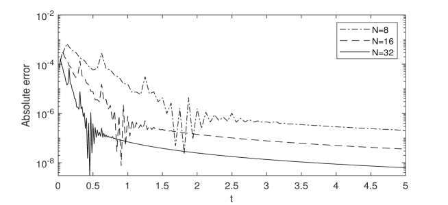
Fig. 4: Pointwise errors of BGACQ_1,2 for Eq. (42) with various N.

Fig. 5: Pointwise errors of MBGACQ_1,2 for Eq. (42) with various N.

Table 14: Errors and convergence rates of MBGACQ${}_{k_{1},k_{2}}$ for Eq. (42) with $m=10.$

  $N$ $(k_{1},k_{2})=(1,1)$ $(k_{1},k_{2})=(1,2)$ $(k_{1},k_{2})=(1,3)$ $\mathrm{Err}_{N}$ $\mathrm{Order}$ $\mathrm{Err}_{N}$ $\mathrm{Order}$ $\mathrm{Err}_{N}$ $\mathrm{Order}$ 8 $4.46\times 10^{-6}$ - $2.80\times 10^{-7}$ - $1.75\times 10^{-8}$ - 10 $1.88\times 10^{-6}$ 3.9 $9.52\times 10^{-8}$ 4.8 $4.80\times 10^{-9}$ 5.8 12 $9.27\times 10^{-7}$ 3.9 $3.92\times 10^{-8}$ 4.9 $1.65\times 10^{-9}$ 5.8 14 $5.08\times 10^{-7}$ 3.9 $1.85\times 10^{-8}$ 4.9 $6.70\times 10^{-10}$ 5.9 16 $3.01\times 10^{-7}$ 3.9 $9.60\times 10^{-9}$ 4.9 $3.05\times 10^{-10}$ 5.9 18 $1.89\times 10^{-7}$ 3.9 $5.38\times 10^{-9}$ 4.9 $1.52\times 10^{-10}$ 5.9  

4.3 Integral Equation With a Rapidly Varying Solution

Finally, let us test the stability of MBGACQ${}_{k_{1},k_{2}}$ by solving the integral equation

(43) $$\int_{0}^{t}k(t-s)u(s)ds=g(t),~{}~{}t\in[0,4],$$

where the Laplace transform of $k(t)$ is selected to be $K(\lambda)=1-\mathrm{e}^{-\lambda}$ and $g(t)=\mathrm{e}^{-100(t-0.5)^{2}}.$ Its exact solution is $u(t)=\sum_{j=0}^{3}g(t-j)$ (see [3]). As a comparison, we also apply BDF2CQ and RKCQs of $3-$stage Radau IIA and $4-$stage Labatto IIIC to solve Eq. (43). The total quadrature nodes of all approaches are set to be fixed 180. Computed results are shown in Figures 6–11. It can be seen that MBGACQ${}_{k_{1},k_{2}}$ is able to accurately solve Eq. (43), while RKCQs and BDF2CQ perform poorly. We conclude that BGACQ${}_{k_{1},k_{2}}$ is much more stable than existing CQs.

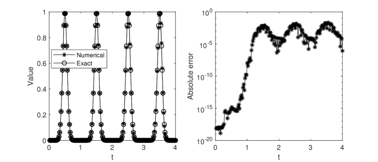
Fig. 6: Computed results of MBGACQ_1,1 for Eq. (43) with 180 quadrature nodes.

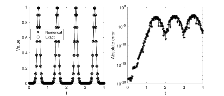
Fig. 7: Computed results of MBGACQ_1,2 for Eq. (43) with 180 quadrature nodes.

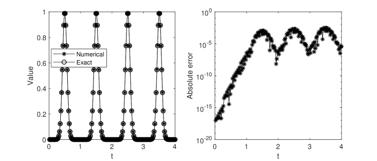
Fig. 8: Computed results of MBGACQ_1,3 for Eq. (43) with 180 quadrature nodes.

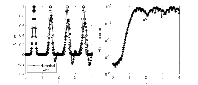
Fig. 9: Computed results of BDF2CQ for Eq. (43) with 180 quadrature nodes.

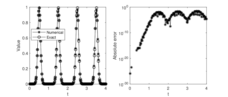
Fig. 10: Computed results of 3-stage Radau IIA RKCQ for Eq. (43) with 180 quadrature nodes.

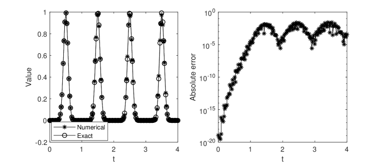
Fig. 11: Computed results of 4-stage Lobatto IIIC RKCQ for Eq. (43) with 180 quadrature nodes.

5 Conclusions

Up to now, we have described a class of multistage CQs with the help of the block generalized Adams method. The analysis in Section 2 indicates using the block generalized Adams method enables the resulting algorithm to efficiently compute CI (1). According to the numerical results, it is evident that BGACQ allows for the stable calculation with a large integration interval. Besides, the proposed CQ works well as the approximation to integral equations. Therefore, we can foresee that the proposed CQ has a great potential to numerical studies on fractional differential equations, time-domain boundary integral equations, Volterra integral equations and so on.

References

[1]
Banjai, L.: Multistep and multistage convolution quadrature for the wave equation: algorithms and experiments. SIAM Journal on Scientific Computing, 32(5): 2964–2994 (2010).
[2]
Banjai, L., Lubich, C.: An error analysis of Runge-Kutta convolution quadrature[J]. BIT Numerical Mathematics, 51: 483–496 (2011).
[3]
Banjai, L., Sayas, F.: Integral Equation Methods for Evolutionary PDE: A Convolution Quadrature
Approach. Springer Nature (2022).
[4]
Banjai, L., Ferrari, M.: Runge-Kutta convolution quadrature based on Gauss methods. arXiv preprint, arXiv:2212.07170 (2022).
[5]
Banjai, L., Ferrari, M.: Generalized convolution quadrature based on the trapezoidal rule. arXiv preprint, arXiv:2305.11134 (2023).
[6]
Brugnano, L., Trigiante, D.: Solving Differential Equations by Multistep Initial and Boundary Value Methods. CRC Press (1998).
[7]
Brunner, H.: Collocation Methods for Volterra Integral and Related Functional Differential Equations. Cambridge University Press (2004).
[8]
Brunner, H.: Volterra Integral Equations: An Introduction to Theory and Applications. Cambridge University Press (2017).
[9]
Cuesta, E., Lubich, C., Palencia, C.: Convolution quadrature time discretization of fractional diffusion-wave equations. Mathematics of Computation, 75(254): 673–696 (2006).
[10]
Davies, P., Duncan, D.: Convolution-in-time approximations of time domain boundary integral equations. SIAM Journal on Scientific Computing, 35(1): 43–61 (2013).
[12]
Fischer, M.: Fast and parallel Runge-Kutta approximation of fractional evolution equations. SIAM Journal on Scientific Computing, 41(2): 927–947 (2019).
[14]
Iavernaro, F., Mazzia, F.: Block-boundary value methods for the solution of ordinary differential equations. SIAM Journal on Scientific Computing, 21(1): 323–339 (1999).
[15]
Jin, B., Li, B., Zhou, Z.: Correction of high-order BDF convolution quadrature for fractional evolution
equations. SIAM Journal on Scientific Computing, 39(6): 3129–3152 (2017).
[16]
Jin, B., Li, B., Zhou, Z.: An analysis of the Crank-Nicolson method for subdiffusion. IMA Journal of Numerical Analysis, 38(1): 518–541 (2018).
[17]
López-Fernández, M., Sauter, S.: Generalized convolution quadrature based on Runge-Kutta methods.
Numerische Mathematik, 133(4): 743–779 (2016).
[18]
Lubich, C.: Convolution quadrature and discretized operational calculus. I. Numerische Mathematik,
52(2): 129–145 (1988).
[19]
Lubich, C.: Convolution quadrature and discretized operational calculus. II. Numerische Mathematik,
52(4): 413–425 (1988).
[20]
Lubich, C., Ostermann, A.: Runge-Kutta methods for parabolic equations and convolution quadrature.
Mathematics of Computation, 60(201): 105–131 (1993).
[22]
Melenk, J., Rieder, A.: On superconvergence of Runge-Kutta convolution quadrature for the wave equation. Numerische Mathematik, 147(1): 157–188 (2021).
[24]
Rieder, A., Sayas, F., Melenk, J.: Time domain boundary integral equations and convolution quadrature for scattering by composite media. Mathematics of Computation, 91(337): 2165–2195 (2022).
[25]
Shi, J., Chen, M.: High-order BDF convolution quadrature for subdiffusion models with a singular source term. arXiv preprint, arXiv: 2305.03384 (2023).
[26]
Wang, X., Wildman, R., Weile, D., Monk, P.: A finite difference delay modeling approach to the discretization of the time domain integral equations of electromagnetics. IEEE Transactions on Antennas and Propagation, 56(8): 2442–2452 (2008).
[27]
Xu, K., Austin, A., Wei, K.: A fast algorithm for the convolution of functions with compact support using Fourier extensions. SIAM Journal on Scientific Computing, 39(6): 3089–3106 (2017).
[28]
Xu, K., Loureiro, F.: Spectral approximation of convoution operators. SIAM Journal on Scientific
Computing, 40(4): 2336–2355 (2018).