Purity-Assisted Zero-Noise Extrapolation for Quantum Error Mitigation

Abstract

Quantum error mitigation is a technique used to post-process errors occurring in the quantum system, which reduces the expected errors and achieves higher accuracy. One method of quantum error mitigation is zero-noise extrapolation, which involves amplifying the noise and then extrapolating the observable expectation of interest back to a noise-free point. This method usually relies on the error model of the noise, as error rates for different levels of noise are assumed during the noise amplification process. In this paper, we propose that the purity of output states in noisy circuits can assist in the extrapolation process, eliminating the need for assumptions about error rates. We also introduce the quasi-polynomial model from the linearity of quantum channel for extrapolation of experimental data, which can be reduced to other proposed models. Furthermore, we verify our purity-assisted zero-noise extrapolation by performing numerical simulations and experiments on the online public quantum computation platform, Quafu, to compare it with the routine zero-noise extrapolation and virtual distillation methods. Our results demonstrate that this modified method can suppress the random fluctuation of operator expectation measurement, and effectively reduces the bias in extrapolation to a level lower than both the zero-noise extrapolation and virtual distillation methods, especially when the error rate is moderate.

I Introduction

It is believed that quantum computation should have superiority beyond classical computation for certain problems. However, the realization of a useful quantum computer is difficult because the qubits are vulnerable to the noise of the environment. Thus, fault-tolerant quantum computation is vital to the application of quantum computation. Quantum error correction code (QECC) provides a systematic solution to fault-tolerant quantum computation [1], while whose application requires many physical qubits and error rate should be lower than a threshold [2, 3, 4]. With remarkable progress [5, 6], however, it is challenging for the state-of-the-art technique to meet the requirements for the full implementation of QECCs. Therefore, fault-tolerant quantum computation based on high-precision logic qubits is still a far-reaching task.

In the noisy intermediate-scale quantum era [7], quantum error mitigation (QEM) provides an alternative technique for noise processing. QECCs detect and correct the errors occurring in the quantum process to make sure that there is no error occurring on coded logic qubits. On the contrary, QEMs allow the occurrence of errors, but use some post-processing techniques to reduce the bias between the output information of noisy quantum circuit and the ideal quantum circuit [8, 9, 10].

In recent years, several QEM schemes are proposed, like zero-noise extrapolation (ZNE) [11, 12, 13, 14], probabilistic error cancellation (PEC) [12, 13], symmetry verification methods [15, 16, 17], purification methods [18, 19, 20, 21], and subspace expansion [22]. These methods have been applied in different quantum computation platforms and interesting physics [23, 24, 25, 26, 27, 28, 29, 30, 31, 32, 33, 34, 35, 36, 25]. Besides, there have been some efforts to integrate various QEM schemes in a generalized framework [17, 37, 38, 10, 37]. Among these various error mitigation schemes, the ZNE and PEC are used to deal with quantum circuits, which require specific error models of noise. The PEC method mitigates the error by post-canceling the noise, which is previously estimated from experiments in the selected error basis. Thus, the effectiveness of PEC closely depends on the error model described by the error basis. Recently, an attempt was made to integrate ZNE into the PEC framework [38].

However, the case of the ZNE method is subtle. This method is based on the analyticity of the observable expectation concerning the error rate, which is a general physical condition. The relation to the error model emerges when the error rate is considered. To perform the ZNE, the error should be amplified, and the ideal value is obtained by extrapolating the expectation reversely to the point of zero noise. In the early application, the error is amplified by stretching the time of pulse for each gate [23], and they have to verify that the error is time scalable. This amplification is not suitable for digital quantum gates either. Another implementation is by deliberately adding redundant gates in the circuit [24]. Then, a treatment called unitary folding is put forward [39]. In this method, the circuit evolves forward and backward successively, and the error rate is characterized by the number of folds. Although the amplifications of the error are developed more feasible, the estimation of the error rate is a priori, which has limitations on the noise type. Moreover, for the complex circuit in the experiment, the effect of errors can hardly be parametrized only by a single parameter of error rate.

The universality of the basic idea of the ZNE method is different from the dependency of error rate on the noise type in implementation. In this paper, we try to release the limitation of noise in the ZNE method, by determining the error rate posteriorly from the experiment. Here, we introduce the purity-assisted zero-noise extrapolation (pZNE) method. In specific, we propose that purity can be used to determine the error rate. Moreover, we can perform the extrapolation on the measured purity, instead of the presumed error rates. For the fitting models of experiment data, we derive the quasi-polynomial model from the linearity of the quantum channel, which can be reduced to other proposed models.

This paper is organized as follows. In Sec. II, we review the routine ZNE method and analyze how this method is based on the error model of noise. Then, we show that the purity of the output state can assist the extrapolation in zero-noise error mitigation in Sec. III. We describe the details of pZNE in Sec. IV, including the fitting model, purity estimation methods, and the measurement overhead. We also verify this method by numerical simulations and experiments on Quafu cloud-based quantum computation platform in Sec. V. The conclusion and discussion are given in Sec. VI.

II Zero-noise Extrapolation with Unitary Folding

The ZNE method consists of two steps:

1. Noise amplification: Collecting the raw data of different error rates via measuring on modulated circuits.

2. Extrapolation: Post-processing the experiment data to obtain the mitigated expectation value based on some fitting models.

In this section, we will review the ZNE method, the fitting models, and the noise amplification method of unitary folding. Besides, we discuss how the presumption that the error rate is proportional to the number of folds is based on the error model of noise.

Let the ideal unitary circuit of interest be $\mathcal{U}$. In practice, we cannot perform this circuit exactly, but a noisy one $\mathcal{U}_{\lambda}$ instead. Then the experimental expectation value $\braket{\hat{O}}_{\lambda}=\mathrm{Tr}[\hat{O}\rho_{\lambda}]$ of observable $\hat{O}$ of interest is different from the ideal one $\braket{\hat{O}}_{0}=\mathrm{Tr}[\hat{O}\rho_{0}]$, where $\rho_{\lambda}=\mathcal{U}_{\lambda}(\rho)$ is the noisy output state, and $\rho_{0}=\mathcal{U}(\rho)$ is the ideal output state. Now, we are going to infer the ideal value $\braket{\hat{O}}_{0}$ from some noisy expectation values $\braket{\hat{O}}_{\lambda}$.

This method is inspired by a simple idea that the expectation value $\braket{\hat{O}}_{\lambda}$ is an analytic function of a parameter $\lambda\geq 0$, which characterizes the noise level of noisy circuit $\mathcal{U}_{\lambda}$, and assume $\braket{\hat{O}}_{\lambda}=\braket{\hat{O}}_{0}$ when $\lambda=0$. With the definition of analyticity, the expectation value can be expanded in a power series of $\lambda$ as

$$\braket{\hat{O}}_{\lambda}=O(\lambda)=\sum_{n=0}^{\infty}O_{n}\lambda^{n},$$ (1)

and by definition of $\lambda$, we have $O_{0}=O(0)=\braket{\hat{O}}_{0}$. So by interpolation the function $O(\lambda)$ with expectations $\braket{\hat{O}}_{\lambda_{i}}$ of different error rate $\lambda_{i}$, one can infer the noise-free expectation value $\braket{\hat{O}}_{0}$.

For the number of experimental data is finite, the expansion of $O(\lambda)$ should be truncated at some order $M$ of $\lambda$, which requires that the error rate $\lambda$ should small enough, and this is the polynomial model of function $O(\lambda)$ [11, 12]. Besides, there are also (multi-)exponential model [14]

$$\braket{\hat{O}}_{\lambda}=O(\lambda)=\sum_{a=0}^{M}B_{a}e^{-\gamma_{a}\lambda},$$ (2)

and poly-exponential model [39]

$$\braket{\hat{O}}_{\lambda}=O(\lambda)=e^{f(\lambda)}+O_{\infty},$$ (3)

where $f(\lambda)$ is a polynomial of $\lambda$. These fitting models are put forward under the consideration that the physical observable should be bounded.

Then, the noisy data of different error rates $\lambda_{i}$ is obtained by error amplification. The unitary folding performs the circuit sequence in the experiment

$$\mathcal{U}_{n}=\mathcal{U}_{\lambda}\circ(\mathcal{U}_{\lambda}^{\dagger}\circ\mathcal{U}_{\lambda})^{n}=(\mathcal{U}_{\lambda}\circ\mathcal{U}_{\lambda}^{\dagger})^{n}\circ\mathcal{U}_{\lambda},$$ (4)

where $\circ$ denotes the composition of quantum operations, the corresponding error rate is expected as $\lambda_{n}=(2n+1)\lambda_{0}$, and the resolution is $2\lambda_{0}$. The circuit is shown in Fig. 1. To have a more fine-grained resolution, it can also perform the layer (gate) folding [39], which assumes the gate can be decomposed into layers $\mathcal{U}_{\lambda}=\prod_{i=1}^{d}\circ\mathcal{L}_{i}$, and performs the folding on these layers

$$\mathcal{L}_{i}\mapsto(\mathcal{L}_{i}\circ\mathcal{L}_{i}^{\dagger})^{n}\circ\mathcal{L}_{i}$$ (5)

in the circuit. By doing so, the resolution can be promoted to $2\lambda/d$.

Figure 1: The circuit of unitary folding.

To consider the procedure of unitary folding in more detail, we assume the circuit is a gate only, and set the noise in forward and backward evolutions as

$$\mathcal{U}_{\lambda} =\mathcal{E}_{f}\circ\mathcal{U},$$ (6)

$$\mathcal{U}_{\lambda}^{\dagger} =\mathcal{U}^{\dagger}\circ\mathcal{E}_{b},$$ (7)

which can be interpreted as the definition of the forward error $\mathcal{E}_{f}$ and backward error $\mathcal{E}_{b}$, whose error rate is denoted as $\lambda_{f}$ and $\lambda_{b}$ correspondingly. Then, we formally have

$$\mathcal{U}_{\lambda}\circ\mathcal{U}_{\lambda}^{\dagger}=\mathcal{E}_{f}\circ\mathcal{E}_{b}\equiv\mathcal{E},$$ (8)

thus the noisy gate is

$$\mathcal{U}_{n}=\mathcal{E}_{n}\circ\mathcal{U},$$ (9)

where $\mathcal{E}_{n}=\mathcal{E}^{n}\circ\mathcal{E}_{f}$ is the error channel with the error rate $\lambda_{n}=n\tilde{\lambda}+\lambda_{f}$, where $\tilde{\lambda}$ is the error rate of error channel $\mathcal{E}$.

To obtain $\lambda_{n}=(2n+1)\lambda_{f}$, we should assume $\tilde{\lambda}=2\lambda_{f}$, which is true when the error channel satisfies $\mathcal{E}_{f}=\mathcal{E}_{b}$. However, this assumption is not always realized. (For more details, see Appendix A.) If we approximate $\tilde{\lambda}\approx 2\lambda_{f}$, it will introduce an additional error in the inference of the ideal value $O(0)$ before fitting the data of experiments. Thus, the ZNE method is constrained by the error model of noise. The simplest way to solve this problem is to determine the error rate $\lambda$ from experiments.

III Extrapolation with Purity

Fidelity is always used to witness the difference between the state with an ideal state, however, the ideal state $\rho_{0}$ cannot be prepared precisely for the unavoidable noise in the experiment. Thus, measuring the fidelity of the noisy state and the ideal state requires the classical simulation of the quantum circuit, which is not feasible in general for large systems. In this section, we will describe the idea of using the purity of the output state of the noisy circuit

$$p(\rho_{\lambda})=\mathrm{Tr}|\rho_{\lambda}|^{2}=\mathrm{Tr}(\rho_{\lambda}^{\dagger}\rho_{\lambda})$$ (10)

to reflect the influence of noise in the circuit. The ideal unitary circuit will not influence the purity of the state. We assume the error is not unitary, otherwise, it can be canceled by the folding of the well-calibrated circuit. Then, the influence of noise on the observable expectation is reflected by the influence on the purity.

In the unitary folding, the folded channel, which is denoted as $\chi$ here, defines a homogenous linear difference equation

$$\rho(x+1)=\chi(\rho(x)),$$ (11)

in the matrix space, where $x$ is a continuous variable of the folding number $n$, which is proportional to the error rate $\lambda$, and we call $x$ also as error rate in the following. Therefore, the phase flow of this equation $g^{x}:\rho(0)\mapsto g^{x}\rho(0)=\rho(x)$, is determined by the channel $\chi$ completely. The extrapolation is actually to infer the ideal expectation along the phase flow where the ideal output state $\rho(0)$ is located.

For the error amplification procedure via unitary folding, we consider the following two folding sequences

$$\tilde{\mathcal{U}}_{n} =(\mathcal{U}_{\lambda}^{\dagger}\circ\mathcal{U}_{\lambda})^{n},$$ (12)

$$\mathcal{U}_{n} =(\mathcal{U}_{\lambda}\circ\mathcal{U}_{\lambda}^{\dagger})^{n}\circ\mathcal{U}_{\lambda}.$$ (13)

There are two different folded channels $\mathcal{U}_{\lambda}^{\dagger}\circ\mathcal{U}_{\lambda},\mathcal{U}_{\lambda}\circ\mathcal{U}_{\lambda}^{\dagger}$, which correspond to two different phase flows. In the folding sequence of $\tilde{\mathcal{U}}_{n}$, the noise-free state is located at $n=0$, but this sequence contains no information of ideal evolution $\mathcal{U}$. Therefore, we should extrapolate the expectation following this sequence to the noise-free point, but the expectations cannot be measured from this sequence. On the contrary, the folding sequence $\mathcal{U}_{n}$ contains the information of ideal channel $\mathcal{U}$, while the noise-free point is not located in its phase flow. Although we can obtain the expectations of observable, we cannot extrapolate to the noise-free point following this sequence.

The purity of the output state can connect the phase flows of the two folding sequences. With the forward and backward errors defined above, we have

$$\mathcal{U}_{n} =\mathcal{E}_{n}\circ\mathcal{U},$$ (14)

$$\tilde{\mathcal{U}}_{n} =\mathcal{U}^{\dagger}\circ\tilde{\mathcal{E}}_{n}\circ\mathcal{U},$$ (15)

where

$${\mathcal{E}}_{n} =(\mathcal{E}_{f}\circ\mathcal{E}_{b})^{n}\circ\mathcal{E}_{f},$$ (16)

$$\tilde{\mathcal{E}}_{n} =\mathcal{E}_{b}\circ\mathcal{E}_{n-1}=(\mathcal{E}_{b}\circ\mathcal{E}_{f})^{n}.$$ (17)

Now, we consider another sequence

$$\breve{\mathcal{U}}_{n}=\tilde{\mathcal{E}}_{n}\circ\mathcal{U},$$ (18)

where the noise-free point is located and the information of forward circuit $\mathcal{U}$ is maintained. This sequence is suitable for our extrapolation, but cannot be performed via the unitary folding technique. However, the purity of the output state of this circuit sequence

$$p\left(\breve{\mathcal{U}}_{n}(\rho)\right)=p\left(\tilde{\mathcal{U}}_{n}(\rho)\right)$$ (19)

is same as the sequence $\tilde{\mathcal{U}}_{n}$, for purity is invariant under unitary evolution. This allowed us to label the phase flow of $\breve{\mathcal{U}}_{n}(\rho)$ with purity measured from the experiment. The error rate of $\breve{\mathcal{U}}_{n}$ is $x=n$ without problem when $x=0$ denotes the noise-free point, and purity of output state of $\tilde{\mathcal{U}}_{n}$ allows us to find the function $p(x)$ on the phase flow of the sequence $\breve{\mathcal{U}}_{n}$. Then, the error rate ${x}_{n}$ of $\mathcal{U}_{n}$ should satisfy

$$p({x}_{n})=p\left(\mathcal{U}_{n}(\rho)\right),$$ (20)

where the purity $p\left(\mathcal{U}_{n}(\rho)\right)$ can be measured from experiments. Particularly, the difference $\lambda_{n}={x}_{n}-{x}_{n-1}$ of error rate should not be uniform for different $n$ in general. With the value of ${x}_{n}$, we can fit the curve of expectation $O(x)$ versus error rate $x$ with the experimental data $O({{x}_{n}})=\mathrm{Tr}(\hat{O}\mathcal{U}_{n}(\rho))$ to the noise-free point $x=0$.

However, solving the error rate ${x}_{n}$ from purity is not an easy task. We can extrapolate to the noise-free point directly on the purity instead. To do so, we measure the purity $p(0)$ of the noise-free state from the circuit $\tilde{\mathcal{U}}_{0}$ without evolution ${\mathcal{U}}_{\lambda}$. This purity $p(0)$ describes the error occurring in the procedure of preparation and measurement, which cannot be amplified by unitary folding. Here, we should assume the noise of preparation and measurement is mitigated beforehand. The reason we measure the noise-free state purity $p(0)$ is that we cannot always assume the initial state is always a pure state. However, if the ideal state is a pure state, we can assume $p(0)=1$, and the above procedure can be interpreted as a way to “purify” the noisy state. Different from the QEM method of purification, which virtually purifies a mixed state to the pure state closest to it, here the noisy state is virtually purified along the phase flow of the noise. (For information on the purification method, see Appendix B.)

IV Details of Methods

In Sec. III, we discuss the procedure of the pZNE method. Different from the routine ZNE method, the pZNE method requires measurement of purity to determine the error rate. In the following, we will show more details of pZNE in practice, including the specific fitting model and purity estimation. Besides, we will also discuss the measurement overhead of this mitigation scheme.

IV.1 Fitting model

With the assumption of the analyticity of the expectation $O(x)$ concerning the error rate $x$, we can expand it into a power series. However, the experiment data are finite, thus it should be truncated as a polynomial. This model is not perfect, since it is in effect only when the error rate is small enough. Moreover, when error rate $x\rightarrow\infty$, the polynomial fitting model will give divergence also. But, the state $\rho(\infty)$ is still normalized, thus $O(\infty)=\mathrm{Tr}[\hat{O}\rho(\infty)]\leq\|\hat{O}\|_{\infty}$, where $\|\hat{O}\|_{\infty}$ is the spectrum radius, the supremum of moduli of eigenvalues, of the observable $\hat{O}$. The spectrum radius of the observable $\hat{O}$ of finite dimension quantum system, qubits or qudits, are always finite. Even in the continuous quantum system, which allows the infinity spectrum radius, the infinity is not a real experience, but a limit. Thus, the boundedness of the physical observable is convinced. The simplest fitting model, the exponential model, with the additional assumption of boundedness is proposed, and then the multi-exponential model and the poly-exponential model.

Although all these models are reasonable, we can derive the fitting model in more detail. Here, we notice that all the quantum channels (without post-selection) are linear, which gives a homogenous linear difference equation, namely Eq. (11). With this property, we conclude from the theory of linear differential equation that the solutions are linear combinations of quasi-polynomials $q_{k}(x)=P_{k}(x)e^{kx}$, where $P_{k}(x)$ are polynomials. Then, we show the details.

In an orthonormal basis $\ket{i}$, we choose the matrix basis $M_{i}^{\,j}\equiv\ket{i}\bra{j}$ with the multiplication rule $M_{i}^{\,j}M_{k}^{\,l}=\delta_{k}^{\,j}M_{i}^{\,l}$. With this basis, we expand the super-operators $\chi$ as

$$\mathcal{\chi}(\rho)=\chi^{i\,k}_{\,j\,l}M_{i}^{\,j}\rho M_{k}^{\,l},$$ (21)

and density matrix

$$\rho=\rho^{m}_{\,n}M_{m}^{\,n}.$$ (22)

Here we adopt the Einstein convention that repeated index means summation. By simple calculation, we get the tensor representation of super-operator on operators

$$\mathcal{\chi}(\rho)^{i}_{\,j}=\chi^{i\,n}_{\,m\,j}\rho^{m}_{\,n}.$$ (23)

It is possible to rephrase this representation in the more familiar form of the vector [40], which just raises the “bra” index of the density matrix, thus we are still working in the tensor here.

We now consider the phase flow defined by a channel $\chi$ in the matrix space

$$\rho^{i}_{\,j}(x+1)=\chi^{i\,n}_{\,m\,j}\rho^{m}_{\,n}(x),$$ (24)

where $\chi^{i\,n}_{\,m\,j}$ is the tensor of channel $\chi$. There exists a “unitary” transformation $u$, which preserves the inner product $(\hat{A},\hat{B})=\mathrm{Tr}(\hat{A}^{\dagger}\hat{B})$ of matrix space, transform the tensor $\chi$ into Jordan canonical form, in some orthonormal matrix basis. This transformation preserves the Frobenius norm of the density matrix, namely the square root of purity $p(\rho)$, but not the trace, thus may be non-physical. Notice that the unitary transformation is performed on density matrix $\rho^{m}_{\,n}$, which only preserves the norm of purity $p(\rho)$ of density, but not the trace, thus may not be physical. Under this transformation, the density $\rho^{i}_{\,j}$ is transformed into a non-normalized “state” $\tilde{\rho}^{i}_{\,j}$, which is the root vector of $\chi$, thus has the form of quasi-polynomial (see Appendix C)

$$\tilde{\rho}^{i}_{\,j}(x)=\tilde{\chi}_{ij}^{x}P_{ij}(x),$$ (25)

where $\tilde{\chi}_{ij}$ are the eigenvalues of $\chi$, and $P_{ij}(x)$ are polynomials whose degree are less than the order of corresponding eigenvalues $\mathrm{ord}\tilde{\chi}_{ij}$. Since it is possible that some eigenvalues are the same, we reorder them as $\tilde{\chi}_{a}$, where $a$ runs from $0$ to $M$, and in the original basis the density matrix is a linear combination of these quasi-polynomials

$$\rho^{i}_{\,j}(x)=\sum_{a}P^{\ i}_{a\,j}(x)\tilde{\chi}_{a}^{n}.$$ (26)

On the other hand, because the unitary transformation $u$ preserves the norm of purity, the purity is also the linear combination of quasi-polynomials

$$p(\chi^{n}(\rho))=p(\tilde{\chi}^{n}(\tilde{\rho}))=\sum_{a}A_{a}(x)|\tilde{\chi}_{a}|^{2n},$$ (27)

where $\deg A_{a}<2\mathrm{ord}\tilde{\chi}_{a}$. Since the purity is over the bounded range $[1/d,1]$, $|\tilde{\chi}_{a}|\leq 1$ must be satisfied. Defining $k_{a}$ satisfying $e^{-k_{a}}=\tilde{\chi}_{a}$, we get the quasi-polynomials model of observable and purity

$$O(x) =\sum_{a=1}^{M}B_{a}(x)e^{-k_{a}x}+B_{0},$$ (28)

$$p(x) =\sum_{a=1}^{M}A_{a}(x)e^{-2\Re(k_{a})x}+A_{0},$$ (29)

where $k_{0}=0$, $\Re(k_{a})$ is the real part of $k_{a}$, $B_{a}=O_{i}^{\,j}P^{\ i}_{a\,j}$, and $O_{i}^{\,j}$ is the matrix element of operator $\hat{O}$. The reason the polynomials $A_{0}$ and $B_{0}$ have zero degrees is that otherwise, they will be divergent at infinity. In the large error limit $x\rightarrow\infty$, the state can be set as the maximal mixed state $I/d$, thus $A_{0}=1/d,B_{0}=\mathrm{Tr}[\hat{O}/d]$, or we can fit $A_{0},B_{0}$ from experiment data.

Now we can fit the experimental data with this quasi-polynomial form as Eqs. (28) and (29). However, the number of eigenvalues and the degree of corresponding quasi-polynomials depend on the specific error, which is unknown, thus we must perform some approximation in practice. For example, we may assume the degree of quasi-polynomials corresponding to each eigenvalue are all the same, and then the number of eigenvalues should be determined by the size of the experiment data. For more simplicity, the degree of quasi-polynomials may be assigned as zero, which reduces to the multi-exponential model. Moreover, by viewing the $n$-th degree coefficients of polynomials with different exponential decay as non-normalized quasi-probabilistic measures of index $a$, by cumulant expansion, the model can be written as

$$O(x)=\sum_{n}x^{n}e^{-v_{n}(x)}+B_{0},$$ (30)

$$p(x)=\sum_{n}x^{n}e^{-u_{n}(x)}+A_{0},$$ (31)

where the coefficients of polynomials $u_{n}(x),v_{n}(x)$ are the cumulants of $k_{a}$. With the approximation that the degree of quasi-polynomials is zero, this model is reduced to the poly-exponential model. Besides, if we assume the decay rate $k_{a}$ of the exponential function is zero, we come back to the polynomial model. Thus, the quasi-polynomial model from the linearity of the quantum channel allows us to unify all the fitting models that have been proposed.

As previously mentioned, we can fit the expectation versus the purity, but the form of the fitting model will be more complex and cannot be explicitly written out here. However, we can write a phenomenological fitting model here. In specific, we represent the purity $p$ as an index $s=\ln\frac{d-1}{dp-1}$, where $d$ is the dimension of the system, so this index $s$ equal to $0$ at pure state, and $\infty$ at maximally mixed state. So, this index is an error-rate-like index, with which we can temporarily write the fitting model as the form of quasi-polynomial by substituting the error rate $x$. For $s$ is not the real error rate, we must generalize the quasi-polynomial model, which can be taken as the form of “quasi-poly-exponential”

$$O(s)=\sum_{j}g_{j}(x)e^{-f_{j}(s)}+B_{0},$$ (32)

where $f_{j}(s),g_{j}(s)$ are some polynomials of $s$. This model can also be reduced to the case of multi-exponential or poly-exponential forms as the approximations used.

IV.2 Purity estimation

In this subsection, we will introduce the purity measurement method. Since purity is not a linear operator of the density matrix, it cannot be easily evaluated in experiments. The most trivial way to measure the purity is to perform the quantum state tomography (QST), and then calculate the purity by definition. However, QST is so expensive that it is hard to perform on a large system. This difficulty may hinder the usage of purity in extrapolation. We can reduce the size of the system we measured. If the operator we care about is located on some sites, we can only measure the purity of these sites. Nevertheless, there may exist the case that we must measure the purity of a relatively large system. Therefore, we need more efficient methods to measure purity.

Figure 2: The circuit of random measurement. The gate $\mathcal{U}_{i}$ is uniformly sampled from an ensemble of unitary gates, like the n-qubit or tensor products of single-qubit Clifford unitaries. The quantum state $\rho$ can be recovered from the n-bit measurement outcome and the choice of the unitary gate $\mathcal{U}_{i}$

The purity can be measured by random measurement [41], where we randomly measure the operators sampled from an ensemble, typically the Pauli string of the qubits. The circuit is shown in Fig. 2. This method is called classical shadow, which can substitute QST. By random measurement of operators with the Monte Carlo sampling, this method is more efficient than QST for large-size systems. The number of measurements is shown in the order of

$$\sim\frac{\log(M)\sup_{i}\|O_{i}\|}{\epsilon^{2}},$$ (33)

which is determined by the observable operators $\hat{O}_{i},(i=1,\dots,M)$ of interest, the ensemble of unitary gates, and the precision $\epsilon$.

Figure 3: The circuit of $\hat{S}^{(M)}$.

In the purification method, the measurement of quantities $\mathrm{Tr}(\rho^{M})$ is the key problem. The measurement method with a replica is proposed, which is founded on the following equation

$$\mathrm{Tr}\left(\hat{O}\rho^{M}\right)=\mathrm{Tr}\left(\hat{O}_{(i)}\hat{S}^{(M)}\rho^{\otimes M}\right),$$ (34)

where $\rho^{\otimes M}$ is $M$ copies of $\rho$, $\hat{O}_{(i)}$ is the operator $\hat{O}$ acted on the $i$-th copy, typically $i=1$, and $\hat{S}^{(M)}$ is cyclic permutation on $M$ copies

$$\hat{S}^{(M)}\ket{\psi_{1}}\otimes\ket{\psi_{2}}\otimes\dots\otimes\ket{\psi_{M}}=\ket{\psi_{2}}\otimes\dots\otimes\ket{\psi_{M}}\otimes\ket{\psi_{1}}.$$ (35)

The purity can be mapped to the expectation of $\hat{S}^{(2)}$ on two-replica state $\rho^{\otimes 2}$. The circuit of $\hat{S}^{(M)}$ is shown in Fig. 3. This method allows us to measure the purity directly from the quantum circuit, which is generally used in the so-called virtual distillation or error suppression by derangement (VD/ESD) in the purification method [19]. Although it can reduce the exponentially increasing quantities measured in QST, it enlarges the space complexity of qubits for the preparation of $2$ copies, and the SWAP gates needed in applying $\hat{S}^{(2)}$ will enlarge the time complexity of the quantum circuit.

IV.3 Extrapolation with echo

(a) $p_{e}$

(b) $p_{f}$

Figure 4: The circuits to measure $p_{e}$ of $p_{f}$ and $\braket{\hat{O}}$ simultaneously for folding gate $\mathcal{U}_{n}$.

Besides the above-mentioned methods in the last subsection, there is a variation of purity estimation called echo or state verification. Inspired by this echo protocol of purification method [17], we modify the extrapolation method. We consider the purity of $\rho(x)=\mathcal{U}_{x}(\rho)$, where $\mathcal{U}_{x}$ is $2x+1$ folds of $\mathcal{U}_{\lambda}$, then the purity of the output state

$$p(x) =\mathrm{Tr}\rho(x)^{2}=\mathrm{Tr}\left[\mathcal{U}_{x}(\rho)^{2}\right]$$

$$=\mathrm{Tr}\left[\rho\left(\mathcal{U}_{x}\right)^{\dagger}\circ\mathcal{U}_{x}(\rho)\right]=\mathrm{Tr}\left[\rho\hat{\rho}_{x}\right],$$ (36)

is the overlap of initial state $\rho$ with quasi-state $\hat{\rho}_{x}=\left(\mathcal{U}_{x}\right)^{\dagger}\circ\mathcal{U}_{x}(\rho)$, which is not physical in general. Here, the $\dagger$ on the channel $\mathcal{U}_{x}$ is acted on its Kraus operators, but not the output state $\mathcal{U}_{x}(\rho)$. For $\mathcal{U}_{x}=(\mathcal{U}_{\lambda}\circ\mathcal{U}_{\lambda}^{\dagger})^{n}\circ\mathcal{U}_{\lambda}$, the quasi-channel is

$$\left(\mathcal{U}_{x}\right)^{\dagger}\circ\mathcal{U}_{x}=\left(\mathcal{U}_{\lambda}\right)^{\dagger}\circ(\mathcal{U}_{\lambda}\circ\mathcal{U}_{\lambda}^{\dagger})^{\dagger n}\circ(\mathcal{U}_{\lambda}\circ\mathcal{U}_{\lambda}^{\dagger})^{n}\circ\mathcal{U}_{\lambda}.$$ (37)

In ideal case, $\lambda=0$, $\left(\mathcal{U}_{\lambda}\right)^{\dagger}=\mathcal{U}_{\lambda}^{\dagger}=\mathcal{U}^{\dagger}$, we have

$$\left.\left(\mathcal{U}_{x}\right)^{\dagger}\circ\mathcal{U}_{x}\right|_{\lambda=0}=\left.\tilde{\mathcal{U}}_{2x+1}\right|_{\lambda=0},$$ (38)

thus we can consider the echo instead

$$p_{e}(x)=\mathrm{Tr}\left[\rho\rho_{x}\right],$$ (39)

where $\rho_{x}=\tilde{\mathcal{U}}_{2x+1}(\rho)$ is a physical state, to determine the error rates. For the ideal state, we measure the ideal echo as $p_{e0}=\mathrm{Tr}[\hat{P}_{0}\rho]=p(\rho)$, which is the purity of the initial state $\rho$, thus the echo is a purity-like quantity.

The echo given above is coincident with the purity if the error channels satisfy

$$\left(\mathcal{E}_{f}\right)^{\dagger}=\mathcal{E}_{b},$$ (40)

which is not satisfied in the general case, but with the assumption that the noise is time independent, this can also be assumed (see Appendix A). However, the advantage is that the echo is easier to measure than purity. Since the initial state can usually reduce to a pure state, and typically, $\ket{0}$, the echo is the recurrence probability

$$p_{e}(x)=\mathrm{Tr}\left[\hat{P}_{0}\rho_{x}\right],$$ (41)

which can be measured from projective measurement. If we want to measure the echo and the observable expectations simultaneously, we can use the non-destructive measurement, like the Hadamard test or phase estimation. In conclusion, to measure the echo, we need not the copy of the system, and the complicated circuit of $\hat{S}^{(M)}$. On the contrary, we lose the universality, as well as, the accuracy to some extent.

As the method described above, we measure the curve of $p=p(x)$ or $p=p_{e}(x)$ to determine the error rate $x$, which is used to extrapolate the expectation $O(x)$. For echo, the inverse function $x=p_{e}^{-1}(p_{e})$ exists in the neighborhood of the zero $x=0$, then the expectation $O(x)$ can locally be written as the function of echo $p_{e}$

$$O(p_{e})=O[p_{e}^{-1}(p_{e})].$$ (42)

Then, we consider another quantity

$$p_{f}(x) =p_{e}(x/2)=\mathrm{Tr}\left[\hat{P}_{0}\tilde{\mathcal{U}}_{x+1}(\rho)\right]$$ (43)

$$=\mathrm{Tr}\left[\rho_{0}\mathcal{E}_{b}\circ\mathcal{E}_{x}(\rho_{0})\right]$$

$$\stackrel{{\scriptstyle x\gg 1}}{{\longrightarrow}}\mathrm{Tr}\left[\rho_{0}\mathcal{E}_{x}(\rho_{0})\right]=\mathrm{Tr}\left[\rho_{0}\rho(x)\right].$$

When $x$ is large enough, the impact of error channel $\mathcal{E}_{b}$ in the last can be ignored, so this quantity approximates the fidelity of noisy state $\rho(x)$ with the ideal state $\rho_{0}$, which is a pure state. With this quantity, we can get the error rate near $x=0$ locally as

$$x=p_{f}^{-1}(p_{f})=2p_{e}^{-1}(p_{f}).$$ (44)

Assume the quantity of ideal state $p_{e0}=\mathrm{Tr}[\hat{P}_{0}\rho]$ is measured the same as the case of echo, then the ideal error rate is

$$x_{0}=p_{e}^{-1}(p_{e0})=\frac{1}{2}p_{f}^{-1}(p_{e0}).$$ (45)

So, the expectation

$$O(p_{f})=O[p_{f}^{-1}(p_{f})]$$ (46)

is extrapolated to

$$p_{f0}=p_{f}\left(\frac{1}{2}p_{f}^{-1}(p_{e0})\right)$$ (47)

The reason we use the quantity $p_{f}(x)$ is that for the folding gate with odd $m=2n+1$ layers, the depth of the circuit to measure the $p_{e}$ is $2m$ layer, while $p_{f}$ with $m+1$. Therefore, the time complexity of quantum circuits measuring $p_{f}$ is less than $p_{e}$. The circuits are shown in Fig. 4.

IV.4 Efficiency

In this subsection, we consider the overhead [9, 17] of extrapolation assisted with purity. The overhead depends on the fitting model, and here, we abstractly denote the fitting model as

$$O_{em}=O(0)=F(\{p_{i},O_{i}\}),$$ (48)

where $F(\{p_{i},O_{i}\})$ is a function of the data $\{p_{i},O_{i}\}$ of purity and observable expectation from the experiment. Then, we calculate the overhead $C_{em}$ of pZNE.

Since the estimator $O_{em}$ is not linear, the variance is not defined rigidly. But up to linear order, we can derive it approximately.

$$\mathrm{Var}[O_{em}]\sim\ \mathrm{Var}[\Delta F]$$ (49)

$$=\mathrm{Var}\left[\sum_{i}\left(\frac{\partial F}{\partial O_{i}}\Delta O_{i}+\frac{\partial F}{\partial p_{i}}\Delta p_{i}\right)\right]$$

$$=\sum_{i}\left(\frac{\partial F}{\partial O_{i}}\right)^{2}\mathrm{Var}[O_{i}]+\left(\frac{\partial F}{\partial p_{i}}\right)^{2}\mathrm{Var}[p_{i}]$$

$$\sim\mathrm{Var}[O]\sum_{i}\left(\frac{\partial F}{\partial O_{i}}\right)^{2}+\mathrm{Var}[p]\sum_{i}\left(\frac{\partial F}{\partial p_{i}}\right)^{2}.$$ (50)

According to the law of large numbers (LLN), the overhead is given by

$$C_{em} \equiv\frac{N^{\epsilon}(O_{em})}{N^{\epsilon}(O)}=\frac{\mathrm{Var}[O_{em}]}{\mathrm{Var}[O]}$$

$$\sim\sum_{i}\left(\frac{\partial F}{\partial O_{i}}\right)^{2}+\frac{\mathrm{Var}[p]}{\mathrm{Var}[O]}\sum_{i}\left(\frac{\partial F}{\partial p_{i}}\right)^{2}$$

$$\sim C_{em}^{\textrm{ZNE}}+\frac{\mathrm{Var}[p]}{\mathrm{Var}[O]}\sum_{i}\left(\frac{\partial F}{\partial p_{i}}\right)^{2},$$ (51)

where $N^{\epsilon}(O_{em})$ and $N^{\epsilon}(O)$ is the number of shots to measure the mitigated estimator $O_{em}$ and the raw estimator $O$ up to $\epsilon$ precision correspondingly. Here, we assume the overhead of routine ZNE method $C_{em}^{\textrm{ZNE}}\sim\sum_{i}\left({\partial F}/{\partial O_{i}}\right)^{2}$ approximates to the observable expectation part of the overhead of pZNE. The reason is that the purity influences the mitigated estimator $O_{em}$ via the error-rate-like index $s$, thus the fitting model $O(s)$ is similar to the one $O(x)$ of ZNE.

In the second term of the overhead $C_{em}$, the part depending on $F$ is correlated to the specific fitting model. We only consider the variance $\mathrm{Var}[p]$ of purity in the latter. The variance $\mathrm{Var}[p]$ depends on the method to measure the purity, and as we previously discussed, there are two kinds of methods to measure the purity. One is the replica measurement method, which is based on the Eq. (34). Another one is the QST-like method, QST and classical shadow, which measure the expectation of all Pauli operators $\braket{\hat{\sigma}_{\alpha}}$, where $\alpha\in\{1,2,\dots,4^{L}-1\}$, and $L$ is the subsystem size of interest. The definition of the purity is

$$p=\frac{1}{2^{L}}\left(1+\sum_{\alpha}\braket{\hat{\sigma}_{\alpha}}^{2}\right).$$ (52)

Then, we calculate the overhead of these two different measurement methods respectively.

For the replica measurement method, the variance of purity is

$$\mathrm{Var}[p]=\frac{1}{N}\mathrm{Var}\left[\hat{S}^{(2)}\right]=\frac{1-p^{2}}{N}.$$ (53)

Next, if we assume the observable of interest is a Pauli operator, we have $\mathrm{Var}[O]=\frac{1-O^{2}}{N}$, thus

$$\frac{\mathrm{Var}[p]}{\mathrm{Var}[O]}=\frac{1-p^{2}}{1-O^{2}}.$$ (54)

When the error rate $x\rightarrow 1$, we have $p\rightarrow 1$, if $O\not\rightarrow 1$, then the second term of the overhead $C_{em}$ has less influence, and we have

$$C_{em}\sim C_{em}^{\textrm{ZNE}}.$$ (55)

In the contrary, if $O\rightarrow 1$ also, with Eq. (28) and (29), we have

$$\frac{\mathrm{Var}[p]}{\mathrm{Var}[O]}\rightarrow\frac{1-p}{1-O}\rightarrow\frac{2K_{A}}{K_{B}}\equiv 2\kappa<\infty,$$ (56)

where $K_{A}\equiv\sum_{a}A_{a}(0)\Re(k_{a})$, and $K_{B}\equiv\sum_{a}B_{a}(0)k_{a}=\sum_{a}\tilde{B}_{a}(0)\Re(k_{a})$. The second equality of $K_{B}$ is because that $O=\braket{\hat{O}}$ is real. Then the overhead is

$$C_{em}^{\textrm{ZNE}}\lesssim C_{em}\lesssim C_{em}^{\textrm{ZNE}}+2\kappa\sum_{i}\left(\frac{\partial F}{\partial p_{i}}\right)^{2}.$$ (57)

For the QST-like measurement method, we assume the observable $\hat{O}$ is a Pauli operator located on $L$ qubits, namely $\hat{O}$ is not identity $\hat{I}$ exactly on $L$ qubits, and we call it $L$-weight Pauli operator in below. Then, the variance of purity of these $L$ qubits is

$$\mathrm{Var}[p] =\mathrm{Var}\left[\sum_{\alpha}\frac{\partial p}{\partial\sigma_{\alpha}}\Delta\sigma_{\alpha}\right]=\sum_{\alpha}\left(\frac{\partial p}{\partial\sigma_{\alpha}}\right)^{2}\mathrm{Var}[\sigma_{\alpha}]$$

$$=\frac{1}{4^{L-1}}\sum_{\alpha}\braket{\hat{\sigma}_{\alpha}}^{2}\mathrm{Var}[\sigma_{\alpha}].$$ (58)

We measure the $3^{L}$ different $L$-weight Pauli operators with the same number $N_{L}$ of shots to perform the QST-like method. To estimate the $l$-weight Pauli operator shorter than $L$, the measurement results of $L$-weight Pauli operators, which have the same components of $\{X,Y,Z\}$ on the nontrivial $l$ qubits as $l$-weight operator, can be used, namely $N_{l}=3^{L-l}N_{L}$. Thus, by LLN, the variance of the $l$-weight Pauli operator is

$$\mathrm{Var}[\sigma_{|\alpha|=l}]\sim\frac{N_{L}}{N_{l}}\mathrm{Var}[\sigma_{|\alpha|=L}]=3^{l-L}\mathrm{Var}[O].$$ (59)

Dividing the summation of $\alpha$ into the summation of weight $|\alpha|=l$, we have

$$\mathrm{Var}[p] =\frac{1}{4^{L-1}}\sum_{l>0}3^{l}C_{L}^{l}\overline{\braket{\hat{\sigma}{\alpha}{=l}}{}{2}}\mathrm{Var}[\sigma_{|\alpha|=l}]$$

$$\sim\frac{\mathrm{Var}[O]}{4^{L-1}}\sum_{l>0}3^{2l-L}C_{L}^{l}\overline{\braket{\hat{\sigma}{\alpha}{=l}}{}{2}}$$

$$\lesssim\frac{4\mathrm{Var}[O]}{12^{L}}\sum_{l>0}3^{2l}C_{L}^{l}=\frac{4(10^{L}-1)}{12^{L}}\mathrm{Var}[O],$$ (60)

where $\overline{\braket{\hat{\sigma}{\alpha}{=l}}{}{2}}\equiv\frac{1}{3^{l}C_{L}^{l}}\sum_{|\alpha|=l}\braket{\hat{\sigma}_{\alpha}}^{2}\leq 1$. Therefore, the overhead is bounded as

$$\tilde{C}_{em}^{\textrm{ZNE}}\lesssim C_{em}\lesssim\tilde{C}_{em}^{\textrm{ZNE}}+\frac{4(10^{L}-1)}{12^{L}}\sum_{i}\left(\frac{\partial F}{\partial p_{i}}\right)^{2}.$$ (61)

When $L\rightarrow\infty$, the second term in the rightest inequality goes to zero, which means that the overhead

$$\lim_{L\rightarrow\infty}C_{em}\sim\tilde{C}_{em}^{\textrm{ZNE}}.$$ (62)

This result is actually of intuition, which states that the Pauli operators of higher weight have more contribution to purity [10], thus the variance of purity $\mathrm{Var}[p]$ is well controlled by the variance of the highest weighted Pauli operator $\mathrm{Var}[O]$. However, we note that the overhead of ZNE $\tilde{C}_{em}^{\textrm{ZNE}}$ here is calculated under the assumption that the expectation of $\braket{\hat{O}}$ is measured from QST-like method. In the ZNE method, we need not perform QST to measure $\braket{\hat{O}}$, thus the real ZNE overhead is

$$C_{em}^{\textrm{ZNE}}\sim 3^{-L}Z\tilde{C}_{em}^{\textrm{ZNE}},$$ (63)

where $Z$ is the number of different $L$-weight operators $\hat{O}_{i}$ of interest. Therefore, the overhead asymptotically is

$$\lim_{L\rightarrow\infty}C_{em}\sim\frac{3^{L}}{Z}C_{em}^{\textrm{ZNE}}.$$ (64)

From this result, we find that the more the operators of interest are, and the smaller the subsystem the operators located in is, the more efficient the pZNE is.

V Verification

Figure 5: Simulation result mitigated by pZNE of the expectation $\braket{\hat{Z}_{0}}$ with the output state of CNOT gate for initial state $\ket{00}$. The fitting model is an exponential model. The error model is the depolarizing error, with different error rates $q$. For each error rate, three instances of folding sequence are sampled for fitting, and the folded number $\Delta N$ between each sample is different for different error rates. The purity and observable are measured by QST, where each Pauli basis of $2$-weight is measured with $1000$ shots.

(a) Circuit

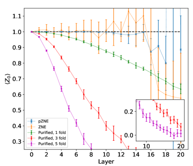
(b) Mitigated expectation

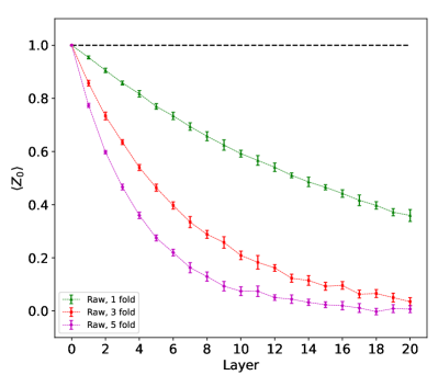
(c) Raw expectation

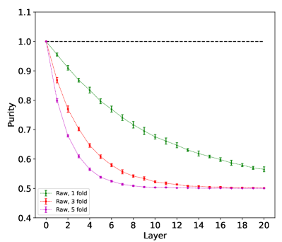
(d) Purity

Figure 6: The numerical simulation of pZNE, ZNE, and VD/ESD with the depolarizing error $\mathcal{D}_{q}$, where error rate $q=0.05$ per gate. The circuit is shown in LABEL:sub@subfig:_run_circuit, which includes several layers of folded noisy CNOT gate $\mathcal{U}_{n}$. Each circuit is simulated with $10$ repetitions, and the QST results are obtained by performing $1000$ single-shot measurements on each $2$-weight Pauli basis. The mitigated expectations of pZNE, ZNE, and VD/ESD are shown in LABEL:sub@subfig:_run_error. The raw data of expectation $\braket{\hat{Z}_{0}}$ and purity are shown in LABEL:sub@subfig:_run_raw and LABEL:sub@subfig:_run_purity.

(a) Circuit

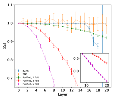
(b) Mitigated expectation

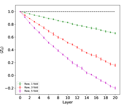
(c) Raw expectation

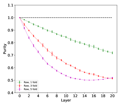
(d) Purity

Figure 7: The numerical simulation of pZNE, ZNE and VD/ESD with the thermal relaxation error $\mathcal{T}$, where the ground state is $\ket{11}$, the relaxation times of the $0$th qubit are $T_{10}=54.5\mu s,T_{20}=4.8\mu s$, the relaxation times of the $1$st qubit are $T_{11}=33.6\mu s,T_{21}=5.3\mu s$, and the gate time is $T_{\textrm{gate}}=0.5\mu s$. The circuit is shown in LABEL:sub@subfig:_run_circuit, which consists of layers of folded noisy CNOT gate $\mathcal{U}_{n}$. Each circuit is simulated with $10$ repetitions, and the QST results are obtained by performing $1000$ single-shot measurements on each $2$-weight Pauli basis. The mitigated expectations of pZNE, ZNE, and VD/ESD are shown in LABEL:sub@subfig:_run_error. The raw data of expectation $\braket{\hat{Z}_{0}}$ and purity are shown in LABEL:sub@subfig:_run_raw and LABEL:sub@subfig:_run_purity.

(a) Circuit

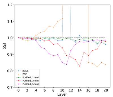
(b) Mitigated expectation

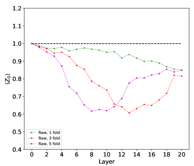
(c) Raw expectation

(d) Purity

Figure 8: The experimental simulation of pZNE, ZNE, and VD/ESD. The circuit is shown is LABEL:sub@subfig:_exper_circuit, which consists of layers of folded noisy CNOT gate $\mathcal{U}_{n}$, where the noise $\mathcal{E}$ is determined by the experiment device. The expectation $\braket{\hat{Z}_{0}}$ with the initial state $\ket{00}$ under increasing CNOT gate folding layers is shown. The fitting model is an exponential model. Each Pauli basis is repeatedly measured with $1000$ shots. The mitigated expectations of pZNE, ZNE, and VD/ESD are shown in LABEL:sub@subfig:_run_error. The raw data of expectation $\braket{\hat{Z}_{0}}$ and purity are shown in LABEL:sub@subfig:_run_raw and LABEL:sub@subfig:_run_purity.

In this section, we simulate the pZNE method numerically and experimentally.

V.1 Numerical simulation: depolarizing error

First, we verify the effectiveness of pZNE by numerical simulation. The CNOT gates under the depolarizing error of different error rates are simulated. The initial state is selected as the $\ket{00}$ state, and the observable expectation $\braket{\hat{Z}_{0}}$ of Pauli $Z$ operator on the qubit $q_{0}$ is measured to present the effect of the error. For an ideal CNOT gate, the expectation $\braket{\hat{Z}_{0}}=1$ is invariant for any number of folds. However, the depolarizing error will lead to the decay of the expectation. The mitigated expectation of pZNE is close to the ideal expectation $\braket{\hat{Z}_{0}}=1$. The result is shown in Fig. 5. The decay of expectation well accords with the theoretical result of the relation between expectation and purity

$$\braket{Z_{0}}=e^{-\frac{1}{2}s}=\left(\frac{dp-1}{d-1}\right)^{\frac{1}{2}},$$ (65)

which is derived from the depolarizing error model.

Then, we compare the pZNE to the routine ZNE method and the VD/ESD method. We still perform the CNOT gate simulated under the depolarizing error as verification. The initial state and the observable are the same as the previous one. Each layer of CNOT gate is a folded gate, with $1,3$ and $5$ CNOT gates. We simulate the circuit with different layers, and show the result in Fig. 6. The estimators of pZNE, ZNE and VD/ESD of $1,3$ and $5$ folded gate are shown in the Fig. 6(b), the raw value of expectations $\braket{\hat{Z}_{0}}$ are shown in the Fig. 6(c), and the purities of the noisy state are shown in the Fig. 6(d). (For details of data processing, see Appendix D.)

Comparing the pZNE with the ZNE, before the $10$-th layer, where the purity of $1$ folded noisy state $p\geq 0.675$ in the Fig. 6(d), the average mitigated data of pZNE are closer to the ideal value than that of ZNE, and the standard deviation of pZNE is much less than ZNE. We note that this reduction of standard deviation is not majorly due to LLN. Because the total number of pZNE is $3$ times of ZNE, and the overhead $C_{em}$ of pZNE is larger than that of ZNE from QST $\tilde{C}_{em}^{\textrm{ZNE}}$. Then, the precision is $\epsilon=\sqrt{\frac{\mathrm{Var}[O_{em}]}{N}}=\sqrt{\frac{C_{em}\mathrm{Var}[O]}{N}}$, and reduction of LLN is

$$\frac{\epsilon_{\textrm{pZNE}}}{\epsilon_{\textrm{ZNE}}} =\sqrt{\frac{N_{\textrm{ZNE}}}{N_{\textrm{pZNE}}}\frac{C_{em}^{\textrm{pZNE}}}{\tilde{C}_{em}^{\textrm{ZNE}}}}\gtrsim\sqrt{\frac{N_{\textrm{ZNE}}}{N_{\textrm{pZNE}}}}$$

$$=\frac{1}{\sqrt{3}}\approx 0.577.$$ (66)

However, the deviation of pZNE is less than ZNE an order of magnitude at least before the $10$-th layers. This is because the measurement of purity and the expectation of $\hat{Z}_{0}$ is not independent, and for the exponential fitting model we used, it will lead to the cancellation of the deviation. (For details, see Appendix D.) This effect has less influence in large system, since the variance of purity will decrease to zero with the increase of the system size. Nevertheless, it suggests that a suitable fitting model of the error will lead the pZNE method more efficient.

After the $11$-th layer, the bias between the average value of pZNE and the ideal value increases, while the standard deviations of pZNE are still much lower than that of ZNE. After the $14$-th layer, where the $3$ and $5$ folded noisy state is close to the completely mixed state, namely $p\approx 0.5$ in Fig 6(d), the bias and the standard deviation of pZNE and ZNE grow rapidly. The reason is that when the $3$ and $5$ folded noisy states are close to the steady state, the completely mixed state, the random fluctuation of measurement will easily lead to the error rate corresponding to the measured expectation and purity deviating from the real error rate. The large inaccuracy of error rates estimation, both the assumption in ZNE and the estimation with purity in pZNE, will increase the bias of extrapolation. Thus, we need more measurements to promote precision. These results show that the mitigated data of pZNE is better than ZNE in the low-error stage.

Comparing the pZNE with the VD/ESD method, we find that when the error is not large, namely in the stage where the purity $p>0.8$, the VD/ESD method works well. When purity is largely deviated from $1$, the mitigated data of VD/ESD have a large deviation from the ideal expectation. This is because the purification method which purifies a noisy state to the pure state closest to that state provides a good estimation of the ideal state only when the error is not large enough. Besides, the standard variance of VD/ESD is not rapidly increasing when the error is large. The overhead of pZNE is in the same order as the VD/ESD, therefore, in the stage where the noise of the circuit is moderate, namely $0.675\leq p\leq 0.8$ in Fig 6, the pZNE method can perform better than both ZNE and VD/ESD method.

V.2 Numerical simulation: thermal relaxation error

We simulate the pZNE method with the thermal relaxation error. We still use the exponential fitting model of $\braket{Z_{0}}$ versus $s$, because Eq. (65) also holds in this case. The results are shown in Fig. 7. The estimators of pZNE, ZNE, and VD/ESD of $1,3$ and $5$ folded gate are shown in the Fig. 7(b), the raw value of expectations $\braket{\hat{Z}_{0}}$ are shown in the Fig. 7(c), and the purities of the noisy state are shown in the Fig. 7(d). (For details of data processing, see Appendix D.)

Same as the depolarizing error, when error is moderate, namely before the $12$-th layer in Fig. 7(b), the bias of pZNE mitigated data between the ideal value is less than both ZNE and VD/ESD. After the $12$-th layer, the bias of average and the standard deviation of pZNE increase rapidly as the depolarizing errors, while the data of ZNE are less influenced. The reason is that in the thermal relaxation error, the steady state is $\ket{0}$, so the expectation $\braket{\hat{Z}_{0}}$ will relax to $-1$, which is not reached in our simulation. Therefore, the random fluctuation of measurement will lead less inaccuracy of error rates in the ZNE method, which only use the expectations. On the other hand, for the thermal relaxation error, the expectation $\braket{\hat{Z}_{0}}$ is a global multivalued function of purify $p$, so pZNE can be used only for moderate error rate, where the expectation is locally single-value function of purity. Otherwise, we should cut the branches. Here, we can define an extended “purity”

$$\tilde{p}_{n}=\mathrm{sgn}(\braket{\hat{Z}_{0}}_{n})\left(p-\frac{1}{d}\right)+\frac{1}{d},$$ (67)

and more generally

$$\tilde{p}_{n}=\mathrm{sgn}\left(\frac{O_{n}-O_{\infty}}{O_{1}-O_{\infty}}\right)\left(p-\frac{1}{d}\right)+\frac{1}{d},$$ (68)

where $O_{n}=\mathrm{Tr}(\hat{O}\rho_{n})$ is the $n$ folded expectation, $O_{1}=\mathrm{Tr}(\hat{O}\rho_{\lambda})$ is the raw expectation without mitigation, and $O_{\infty}={\mathrm{Tr}(\hat{O})}/{d}$ is the expectation of the maximal mixed state. This is a cut of a general branch point crossing the maximal mixed state, however, there are other branches depend on the noise model.

V.3 Experiment

We perform the pZNE and ZNE on the cloud-based superconducting quantum computation platform, Quafu [42]. (For the information of the Quafu platform and device, see Appendix E.) The parameters used in the experiment are the same as those used in the numerical simulation. The result is shown in Fig. 8, where the estimators of pZNE, ZNE and VD/ESD of $1,3$ and $5$ folded gate are shown in the Fig. 8(b), the raw value of expectations $\braket{\hat{Z}_{0}}$ are shown in the Fig. 8(c), and the purities of the noisy state are shown in the Fig. 8(d). The detail of data processing is same as the numerical simulation, except without the calculation of standard deviations.

Different from the simulation, where the depolarizing error or the thermal relaxation error is considered, both the raw data of observable expectation $\braket{\hat{Z}_{0}}$ and purity are not monotonically decreasing with the layer increasing, and in particular, the purity does not reach the minimum value $\frac{1}{d}$. This leads to the undesired behavior of ZNE at the stage where the number of layers is larger than $10$. With the help of purity, the mitigated data of pZNE is closer to the ideal expectation $\braket{\hat{Z}_{0}}=1$, except at the $11$-th layer, where the expectation and purity of $3$ and $5$ folded noisy state are close, while both of them are far from the $1$ folded noisy state.

For the mitigated estimators of VD/ESD method, the result of $1$ folded noisy state is closer to ideal value than the pZNE method. This is because the fidelity of CNOT gate is about 0.989, so the error of $20$ layer of $1$ folded gate is not so large that the purity of noisy state $p\geq 0.8$. When the purity $p<0.8$ in the layers of $3$ and $5$ folded gate, the results of VD/ESD method deviate the ideal expectation $1$. The comparison of experiment result between pZNE and VD/ESD method is consistent with the results of numerical simulations.

VI Conclusion

In this paper, we discuss the method using purity to determine the error rates of noise, which is in principle more accurate than the conventionally presumed error rates in the routine ZNE method. We can perform the pZNE method without the inaccuracy of error rates for the different error models of noise. Thus, this method can ensure the accuracy and the universality. Besides, we derive the quasi-polynomial model of the observable expectation versus error rate from the linearity of the quantum channel. We also show that it can reduce to other proposed models, e.g. the polynomial, multi-exponential, and poly-exponential models.

We calculate the overhead of the pZNE under different methods of purity estimation, including the replica measurement method and the QST-like method. We show that for these estimation methods, the upper bounds of pZNE behave differently. The overhead of the replica measurement method is bounded by the overhead of ZNE adding a finite constant, while the overhead of a QST-like method will increase exponentially with the increasing of subsystem size of interest.

For the exponentially increasing overhead, the pZNE is not efficient for large systems via a QST-like method. However, the complexity of the quantum circuit of the replica measurement method also limits its implementation. Thus, a variant method based on the state verification method is proposed. This method requires a simpler quantum circuit compared to the replica measurement method, but its universality and accuracy may be lost.

In addition, we verify the pZNE method with the numerical simulations under the depolarizing error and the thermal relaxation error, as well as the experiments on the quantum computation platform, Quafu. We compare it with the routine ZNE and the VD/ESD method. The results show that the bias of pZNE is less than both ZNE and VD/ESD when the error rate is moderate. The standard deviation of pZNE is lower than ZNE in numerical simulation when LLN is considered, which implies that a suitable fitting model for the error model will help to cancel the random fluctuations of measurements in pZNE. However, the expectation is a multivalued function of purity, thus it may confine the usage of pZNE only in the stage of moderate noise.

Our results demonstrate that the purity of the noisy state can be used in the ZNE method to evaluate the level of noise, which will reduce the bias of extrapolation. It can be expected that pZNE will reinforce the wide usage of the ZNE method in the NISQ era.

Appendix A The Forward and Backward Errors

In this appendix, we consider the forward and backward Errors in the form of Lindblad equation, with the assumption of time independent errors. The ideal evolution $\mathcal{U}$ can be formally written as $\mathcal{U}=\exp[-\mathrm{i}t\mathcal{H}]$, where the action of the super-operator $\mathcal{H}$ is $\mathcal{H}\rho=[H,\rho]$. Assuming the decoherence error is time invariant, then the noisy evolution can be described by master equation formally

$$\partial_{t}\rho=-\mathrm{i}\mathcal{H}\rho+\lambda\mathcal{L}\rho,$$ (69)

where the Lindblad term $\mathcal{L}\rho$ due to the system-environment interaction in the master equation does not depend on time explicitly. Thus, we can write the noisy evolution as

$$\mathcal{U}_{\lambda}=\exp[-\mathrm{i}t\mathcal{H}+\lambda t\mathcal{L}]$$ (70)

For backward evolution, we substitute $\mathcal{H}$ by $-\mathcal{H}$, and

$$\mathcal{U}_{\lambda}^{\dagger}=\exp[\mathrm{i}t\mathcal{H}+\lambda t\mathcal{L}]$$ (71)

By definitions, the error channels are

$$\begin{split}\mathcal{E}_{f}&=\exp[-\mathrm{i}t\mathcal{H}+\lambda t\mathcal{L}]\exp[\mathrm{i}t\mathcal{H}],\\ \mathcal{E}_{b}&=\exp[-\mathrm{i}t\mathcal{H}]\exp[\mathrm{i}t\mathcal{H}+\lambda t\mathcal{L}],\end{split}$$ (72)

which means that $\mathcal{E}_{f}^{\dagger}=\mathcal{E}_{b}$. The equality of the forward and backward errors means that the forward error $\mathcal{E}_{f}$ is Hermitian, which is generally hard to satisfied, and a sufficient condition is that $[\mathcal{H},\mathcal{L}]=0$.

Appendix B Brief Introduction to Purification Method

The purification method is based on the belief that in practice the output state is always mixed, while the ideal state is a pure state. If the error is not so large, the ideal pure state should not far away from the experimental mixed state. Thus, the pure state closest to the mixed state may be a good approximation of the ideal state, and this state is the aim of the purification method.

Let the mixed state $\rho$ decomposed as

$$\rho=\sum_{n}p_{n}\ket{n}\bra{n},$$ (73)

where $p_{n}$ are the spectrum of the density ordered descendingly, and $\ket{n}$ are the corresponding eigenstates. For some other pure state $\ket{\psi}=\sum_{n}\psi_{n}\ket{n}$, the distance

$$\begin{split}D^{2}(\rho,\ket{\psi})&=\mathrm{Tr}\rho^{2}+1-2\bra{\psi}\rho\ket{\psi}\\ &=\mathrm{Tr}\rho^{2}+1-2\sum_{n}p_{n}|\psi_{n}|^{2}\end{split}$$ (74)

minimizes when $|\psi_{n}|=\delta_{n,0}$, namely the state with the largest probability in the mixed state is the closest pure state. It is clear that if we know the mixed state completely, by diagonalization we can get the closest pure state.

For large system, the dimension of the matrix is too overwhelmed to perform the diagonalization. The better way is to realize the purification by iteration. One of the iteration procedure is the McWeeny purification [43, 34]

$$\rho_{n+1}=3\rho_{n}^{2}-2\rho_{n}^{3}.$$ (75)

In basis which can diagonalize the mixed state, this iteration only maps the spectrum. However, the attractive fixed point of this map is $p=0,1$ and the critical point is $1/2$, thus it has the probability of convergence to $0$ for all eigenvalue, which is not what we desire. Only if there is an eigenvalue $p_{n}$ greater than $1/2$, namely the error is small enough, the purification is working. Another one is the map

$$\rho\mapsto\frac{\rho^{M}}{\mathrm{Tr}\rho^{M}}.$$ (76)

In the diagonal representation, the spectra are mapping as

$$p_{n}\mapsto\frac{p_{n}^{M}}{\sum_{m}p_{m}^{M}}=\frac{1}{1+\sum_{m\neq n}(p_{m}/p_{n})^{M}}.$$ (77)

In the limit $M\rightarrow\infty$, the spectra $p_{n}\rightarrow\delta_{n0}$, since $p_{n}$ is in descending order, which is what pure state we want.

To do the purification, one can perform the tomography of target density, and then iterate the procedure given above on classical computer. However, tomography is expansive for large system, other method is also needed. One can prepare the purified state by post-selection, Other strategy is to realize the purification virtually. The purified state can be approximated as $\frac{\rho^{M}}{\mathrm{Tr}\rho^{M}}$ for some given integer $M$, so the expectation of quantity $\hat{O}$ under the purified state approximate as

$$\braket{\hat{O}}_{\mathrm{p}}\approx\frac{\mathrm{Tr}\left(\hat{O}\rho_{\lambda}^{M}\right)}{\mathrm{Tr}\rho_{\lambda}^{M}}.$$ (78)

If the value $\mathrm{Tr}\left(\hat{O}\rho_{\lambda}^{M}\right),\mathrm{Tr}\rho_{\lambda}^{M}$ can be evaluated from the experiment, the purified expectation value can be obtained.

A method called virtual distillation or error suppression by derangement is proposed [19], which is based on the Eq. (34). where $\rho^{\otimes M}$ is $M$ copies of $\rho$, $\hat{O}_{(i)}$ is the operator $\hat{O}$ acted on the $i$-th copy, typically $i=1$, and $\hat{S}^{(M)}$ is cyclic Thus, $\mathrm{Tr}\left(\hat{O}\rho_{\lambda}^{M}\right)$ and $\mathrm{Tr}\rho_{\lambda}^{M}$ can be measured with $M$ copies of $\rho$. For $\hat{S}^{(M)}$ is cyclic permutation on $M$ copies, the expectation of operator $\hat{O}^{(M)}=\frac{1}{M}\sum_{i}\hat{O}_{(i)}$ is same as the original one

$$\mathrm{Tr}\left(\hat{O}_{(i)}\hat{S}^{(M)}\rho^{\otimes M}\right)=\mathrm{Tr}\left(\hat{O}^{(M)}\hat{S}^{(M)}\rho^{\otimes M}\right).$$ (79)

Since $\hat{O}^{(M)}$ are commute with $\hat{S}^{(M)}$, we can find the common eigenstates as the basis, which allows measuring $\mathrm{Tr}\left(\hat{O}\rho^{M}\right)$ and $\mathrm{Tr}\rho^{M}$ simultaneously. One can measure the expectation $\mathrm{Tr}\left(\hat{O}^{(M)}\hat{S}^{(M)}\rho^{\otimes M}\right)$ and $\mathrm{Tr}\left(\hat{S}^{(M)}\rho^{\otimes M}\right)$ by Hadamard test (see Fig. 9) or by diagonalization [19].

Figure 9: The circuit of Hadamard test of VD/ESD.

For the measurement by diagonalization, in a qubit system, let $\hat{O}$ be the $\hat{Z}$ operator, the eigenstates are just spin waves. Moreover, considering the case with two copies, i.e. $M=2$, the eigenstates states are just the spin singlet and triplet, and the transformation is

$$\hat{B}^{(2)}=\left(\begin{array}[]{cccc}1&0&0&0\\ 0&\frac{1}{\sqrt{2}}&-\frac{1}{\sqrt{2}}&0\\ 0&\frac{1}{\sqrt{2}}&\frac{1}{\sqrt{2}}&0\\ 0&0&0&1\end{array}\right).$$ (80)

Under this transformation,

$$\begin{split}\hat{S}^{(2)}&\rightarrow\frac{1}{2}(1+\hat{Z}_{(1)}-\hat{Z}_{(2)}+\hat{Z}_{(1)}\hat{Z}_{(2)})\\ \hat{Z}^{(2)}&\rightarrow\hat{Z}^{(2)}=\frac{1}{2}(\hat{Z}_{(1)}+\hat{Z}_{(2)}),\end{split}$$ (81)

and we can verify that $\hat{Z}^{(2)}\hat{S}^{(2)}=\hat{Z}^{(2)}$.

Appendix C Quasi-Polynomials

The quasi-polynomials are the basis of solutions of an autonomous linear ordinary differential equation system

$$\frac{d}{dt}X=WX,$$ (82)

where $W$ is a matrix not depending on $t$ and $X$. Any evolution equation of linear systems, typically, time-independent quantum system, can be represented in this form. The solution is

$$X(t)=e^{Wt}X(0).$$ (83)

If the matrix $W$ is Hermitian, it can be diagonalized with the eigenvalues $w_{i}$ by the unitary matrix $U=(u_{ij})$

$$W=U\Lambda U^{\dagger},$$ (84)

where $\Lambda=\mathrm{diag}(w_{1},\dots,w_{n})$. The solution of this system is the multi-exponential function

$$x_{i}(t)=\sum_{j,k}e^{w_{j}t}u_{ij}u_{kj}^{\ast}x_{k}(0),$$ (85)

where $x_{i}$ is the component of vector $X$.

In general, if the matrix $W$ is not Hermitian, we cannot diagonalize the matrix with a unitary matrix but a general invertible matrix. However, if we insist on the unitary transformation, this matrix can be diagonalized as the Jordan canonical form

$$W=U\bigoplus_{i}W_{i}U^{\dagger},$$ (86)

where $W_{i}-w_{i}I$ is a nilpotent matrix

$$(W_{i}-w_{i}I)^{d_{i}}=0,$$ (87)

where $d_{i}$ is the dimension of the matrix $W_{i}$. Therefore, we have

$$W_{i}=w_{i}I+b_{i}N_{i},$$ (88)

where

$$N_{i}=\left(\begin{array}[]{cccc}0&1&\\ &0&\ddots&\\ &&\ddots&1\\ &&&0\end{array}\right)$$ (89)

is a nilpotent matrix of $n_{i}$ dimension, $b_{i}$ is a coefficient. Then, the evolution matrix

$$\exp({Wt})=\bigoplus_{i}e^{w_{i}t}U\exp({b_{i}N_{i}t})U^{\dagger}.$$ (90)

Since $N_{i}$ is nilpotent, we have

$$\exp({b_{i}N_{i}t})=\sum_{n=0}^{n_{i}}\frac{b_{i}^{n}t^{n}}{n!}N^{n},$$ (91)

whose elements are polynomials of the parameter $t$, so the elements $U\exp({b_{i}N_{i}t})U^{\dagger}=(n_{ijk}(t))$ are also polynomial of $t$. The solution

$$x_{i}(t)=\sum_{l,j}e^{a_{l}t}n_{lij}(t)x_{j}(0)$$ (92)

is the linear combination of quasi-polynomials $e^{w_{l}t}n_{kij}(t)$.

Appendix D The detail of numerical simulation

D.1 Data Process

For the extrapolation, we substitute the gates with the folded gates with odd numbers $1,3$ and $5$. Besides, we also simulate the case without any gate to separate the error of the circuit and the error of preparation and measurement. The circuit with layers from $1$ to $20$ is simulated $10$ times. After each circuit with given layers, we perform the projective measurement on each qubit on the basis of all three Pauli operators. Each Pauli operator is measured with $1000$ shots.

With the measurement outcome, we estimate the expectations of all Pauli operators of the subsystem of interest, which is used to calculate the purity of this subsystem. For the operator $\hat{Z}_{0}$, it is estimated from $3000$ shots, while the purity of the $0$-th qubit is estimated from $9000$ shots. For a given number of layers, there are results of four different circuits, whose single layer is $0,1,3$ and $5$ folded gate. The estimator of ZNE is extrapolated to the noise-free gate from the expectation $\braket{\hat{Z}_{0}}$ of $1,3$ and $5$ folded gate, with the exponential fitting model

$$\braket{\hat{Z}_{0}}(x)=Ae^{-kx}+B,$$ (93)

where $(A,k,B)$ are the parameters to be determined, and $x$ is the number of folding, namely $1,3$ and $5$. The estimator of pZNE is extrapolated from the expectation $\braket{\hat{Z}_{0}}$ of $1,3$ and $5$ folded gates, and the purity $p(x)$ of $0,1,3$ and $5$ folded gates. The purity is convert to the error-rate-like parameter $s(x)=-\ln\frac{dp(x)-1}{d-1}$, and then the expectation $\braket{\hat{Z}_{0}}$ of the noise-free gate is extrapolated to the $s(0)$ with the exponential fitting model

$$\braket{\hat{Z}_{0}}(s)=Ae^{-ks}+B.$$ (94)

We fit the parameters $A$, $k$ and $B$ by the least square method.

For the VD/ESD method, we use the state estimator with $M=2$ replica

$$\rho_{\mathrm{p}}(x)=\frac{\rho^{2}(x)}{\mathrm{Tr}\rho^{2}(x)},$$ (95)

where $\rho(x)$ is the noisy state of the qubit $q_{0}$. The estimator of expectation is

$$\braket{\hat{Z}_{0}}_{\mathrm{p}}(x)=\mathrm{Tr}(\hat{Z}_{0}\rho_{\mathrm{p}}(x))=\frac{\mathrm{Tr}[\hat{Z}_{0}\rho^{2}(x)]}{\mathrm{Tr}\rho^{2}(x)}.$$ (96)

It can be verified that $\mathrm{Tr}[\hat{Z}_{0}\rho^{2}(x)]=\mathrm{Tr}[\hat{Z}_{0}\rho(x)]=Z({x})$, thus

$$\braket{\hat{Z}_{0}}_{\mathrm{p}}(x)=\frac{Z(x)}{p(x)}.$$ (97)

Since the expectation $\braket{\hat{Z}_{0}}(x)$ and the purity $p(x)$ of $1,3$ and $5$ folded noisy states are measured in the pZNE method, we can calculate the average and standard deviation of the VD/ESD estimators for the $1,3$ and $5$ folding.

D.2 Stochastic Error of pZNE

For convenience, we assume the parameter $B=0$ in our fitting model, which is reasonable for the depolarizing error, otherwise, the estimators are complex for analytical analysis. With this assumption, the extrapolation is performed only with two points of data, $(x_{1},Z_{1})$ and $(x_{2},Z_{2})$, or $(s_{1},Z_{1})$ and $(s_{2},Z_{2})$, which are measured from $1$ and $3$ folded gates. The expectations of noise-free points are estimated as

$$Z_{0}^{\textrm{ZNE}} =\sqrt{\frac{Z_{1}^{3}}{Z_{2}}},$$ (98)

$$Z_{0}^{\textrm{pZNE}} =\left(\frac{Z_{1}^{s_{2}}}{Z_{2}^{s_{1}}}\right)^{1/(s_{2}-s_{1})}.$$ (99)

The noisy state is $\rho_{i}=q_{i}\rho_{0}+(1-q_{i})I/d$ for $q_{1}=q,q_{2}=q^{3}$, so the average expectation and purity is

$$\bar{Z}_{i} =q_{i}$$ (100)

$$\bar{p}_{i} =(1-1/d)q_{i}^{2}+1/d.$$ (101)

The differential of noise-free estimators at the average value are

$$\mathrm{d}Z_{0}^{\textrm{ZNE}} =\frac{3}{2q}\mathrm{d}Z_{1}-\frac{1}{2q^{3}}\mathrm{d}Z_{2},$$ (102)

$$\mathrm{d}Z_{0}^{\textrm{pZNE}} =\frac{3}{2q}\mathrm{d}Z_{1}-\frac{1}{2q^{3}}\mathrm{d}Z_{2}+\frac{3}{4}\mathrm{d}s_{1}-\frac{1}{4}\mathrm{d}s_{2}.$$ (103)

For $s_{i}=-\ln\frac{dp_{i}-1}{d-1}$ and $p_{i}=\frac{1}{d}\left(1+Z_{i}^{2}+\sum_{\sigma\neq Z}\sigma_{i}^{2}\right)$, we have

$$\mathrm{d}s_{i}=-\frac{d}{(d-1)q_{i}^{2}}\mathrm{d}p_{i}=-\frac{2}{(d-1)q_{i}}\mathrm{d}Z_{1},$$ (104)

where the second equality is from the fact that $\rho_{0}=\ket{0}\bra{0}$, and $\bar{\sigma}_{i}=\bar{Z}_{i}\delta_{\sigma,Z}$. Therefore, we get

$$\mathrm{d}Z_{0}^{\textrm{pZNE}}=\left(1-\frac{1}{d-1}\right)\mathrm{d}Z_{0}^{\textrm{ZNE}},$$ (105)

and the ratio of overhead

$$\frac{C_{em}^{\textrm{pZNE}}}{\tilde{C}_{em}^{\textrm{ZNE}}}\approx\frac{\mathrm{Var}[\mathrm{d}Z_{0}^{\textrm{pZNE}}]}{\mathrm{Var}[\mathrm{d}Z_{0}^{\textrm{ZNE}}]}=\left(1-\frac{1}{d-1}\right)^{2}.$$ (106)

When the dimension of subsystem of interest is $d=2$, the ratio $\frac{C_{em}^{\textrm{pZNE}}}{\tilde{C}_{em}^{\textrm{ZNE}}}\approx 0$ up to linear order.

For more simplicity, the key point is that for the depolarizing error, there is the relation

$$Z_{i}=e^{-\frac{1}{2}s_{i}}=\left(\frac{dp_{i}-1}{d-1}\right)^{\frac{1}{2}},$$ (107)

which is verified by the Fig. 5. Therefore, the exponential fitting model is suitable for the depolarizing error. This result demonstrates the importance of a suitable fitting model for the noise.

D.3 Stochastic Error of pZNE: thermal relaxation error

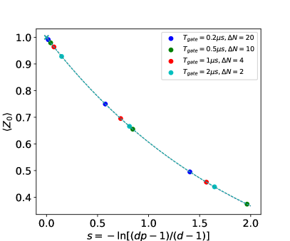
Figure 10: The exponential fitting of the expectation $\braket{\hat{Z}_{0}}$ with purity. The error model is thermal relaxation error, where the ground state is $\ket{11}$, the decoherence times of qubit $q_{0}$ are $T_{10}=54.5\mu s,T_{20}=4.8\mu s$, the decoherence times of qubit $q_{1}$ are $T_{11}=33.6\mu s,T_{21}=5.3\mu s$, and the gate time vary from $T_{\textrm{gate}}=0.2\mu s$ to $2\mu s$. For each error rate, three instances of folding sequence are sampled for fitting, and the folded number $\Delta N$ between each sample is different for different error rates. The purity and observable are measured by QST, where each Pauli basis of $2$-weight is measured with $1000$ shots.

For the thermal relaxation error, the noise state is $\rho_{i}=e^{-\lambda t_{i}}\ket{0}\bra{0}+(1-e^{-\lambda t_{i}})\ket{1}\bra{1}$, where $\lambda$ is a parameter depending on $T_{1}$, so the expectation and the purity are

$$\bar{Z}_{i} =2e^{-\lambda t_{i}}-1,$$ (108)

$$\bar{p}_{i} =2e^{-2\lambda t_{i}}-2e^{-\lambda t_{i}}+1.$$ (109)

It can verify that the expectation and purity also satisfy Eq. (65) with $d=2$ (except the signal of the expectation), which can be verified by simulation (Fig. 10) so we also select the exponential fitting model.

With the assumption that $B^{\textrm{ZNE}}=-1,B^{\textrm{pZNE}}=0$, we can also use two point of data, $(x_{1},Z_{1})$ and $(x_{2},Z_{2})$, or $(s_{1},Z_{1})$ and $(s_{2},Z_{2})$ to estimate the expectations of noise-free point

$$Z_{0}^{\textrm{ZNE}} =\sqrt{\frac{(Z_{1}+1)^{3}}{(Z_{2}+1)}}-1,$$ (110)

$$Z_{0}^{\textrm{pZNE}} =\left(\frac{Z_{1}^{s_{2}}}{Z_{2}^{s_{1}}}\right)^{1/(s_{2}-s_{1})}.$$ (111)

These estimators are similar to the depolarizing error, thus the differentials of $Z_{i}$ can be calculated similarly with $2e^{-\lambda t_{i}}$ substituting $p_{i}$ for ZNE, and $2e^{-\lambda t_{i}}-1$ substituting $p_{i}$ for pZNE. It also has

$$\mathrm{d}Z_{0}^{\textrm{pZNE}}=0,$$ (112)

with the dimension of subsystem of interest $d=2$. Therefore, the ratio $\frac{C_{em}^{\textrm{pZNE}}}{\tilde{C}_{em}^{\textrm{ZNE}}}\approx 0$ up to linear order is also holds.

Appendix E Device Information on Quafu Cloud Platform

In Sec. V, we use the ScQ-P18 device on Quafu cloud platform for experimental verification. Here we utilize the open-source Python SDK, namely PyQuafu, to write the experimental code for running the circuits. The layout of the ScQ-P18 device and the error rates of CZ gates are shown in Fig. 11. We use qubits 0 and 1 on ScQ-P18 for the two-qubit demonstration. The fidelity of their CZ gate is about 0.989. More information about the two used qubits can be found in Table 1.

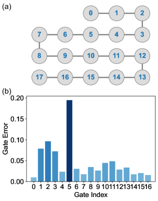
Figure 11: The layout of the chip and the error rates of CZ gates.

Qubit index	0	1
Qubit frequency, $f_{10}$ ($\mathrm{GHz}$)	4.530	5.043
Readout frequency, $f_{r}$ ($\mathrm{GHz}$)	6.776	6.759
Anharmonicity, $\eta$ ($\mathrm{MHz}$)	-204.8	-191.7
Relaxation time, $T_{1}$ ($\mu\mathrm{s}$)	54.7	33.6
Coherence time, $T_{2}$ ($\mu\mathrm{s}$)	4.8	5.2
Readout fidelity of state $\ket{0}$, $F_{0}$	0.954	0.974
Readout fidelity of state $\ket{1}$, $F_{1}$	0.869	0.890

Table 1: The parameters of the two used qubits.

Here we mitigate the readout error of the experimental results on the cloud platform. In specific, we first assume the ideal and noisy measurements are in bases $\ket{x}$ and $\ket{E_{x}}$, respectively. According to the Bayesian readout correction, the relation between the noisy measurement operator $M_{x}:=\ket{E_{x}}\bra{E_{x}}$ and the ideal operator $P_{x}:=\ket{x}\bra{x}$ can be expressed as

$$M_{x}=\sum_{y}R_{xy}P_{y},$$ (113)

where the matrix $R$ can be evaluated from the probability of experimental outcome when performing the noisy measurement on the prepared states $\ket{x}$, namely

$$R_{xy}=\mathrm{Tr}(M_{x}P_{y}).$$ (114)

In the single-qubit case, the matrix $R$ is constructed by the readout fidelities:

$$R=\left(\begin{array}[]{cc}F_{0}&1-F_{1}\\ 1-F_{1}&F_{1}\end{array}\right)$$ (115)

where $F_{0}$ and $F_{1}$ are the readout fidelities of states $\ket{0}$ and $\ket{1}$. Ignoring the readout crosstalk, the multi-qubit $R$ matrix can be reduced to the direct product of each single-qubit $R$ matrix.

With the knowledge of matrix $R$, we can construct the ideal measurement outcome by using its inverse

$$P_{x}=\sum_{y}(R^{-1})_{xy}M_{y},$$ (116)

and the probability $p_{x}=\mathrm{Tr}(P_{x}\rho)$ of some state $\rho$ in state $\ket{x}$ is thus

$$p_{x}=\sum_{y}(R^{-1})_{xy}q_{y},$$ (117)

where $q_{x}=\mathrm{Tr}(M_{x}\rho)$ is the probability of this state in $\ket{E_{x}}$. In addition, we also use the least square method to limit the mitigated probabilities, so that all of them meet the non-negative and normalization conditions.

References

- Terhal [2015] B. M. Terhal, Quantum error correction for quantum memories, Rev. Mod. Phys. 87, 307 (2015).
- Knill et al. [1996] E. Knill, R. Laflamme, and W. Zurek, Threshold accuracy for quantum computation, arXiv:9610011 (1996).
- Aharonov and Ben-Or [1997] D. Aharonov and M. Ben-Or, Fault-tolerant quantum computation with constant error, in Proceedings of the Twenty-Ninth Annual ACM Symposium on Theory of Computing, STOC ’97 (Association for Computing Machinery, New York, NY, USA, 1997) p. 176–188.
- Kitaev [1997] A. Y. Kitaev, Quantum computations: algorithms and error correction, Russian Mathematical Surveys 52, 1191 (1997).
- Zhao et al. [2022] Y. Zhao, Y. Ye, H.-L. Huang, Y. Zhang, D. Wu, H. Guan, Q. Zhu, Z. Wei, T. He, S. Cao, et al., Realization of an error-correcting surface code with superconducting qubits, Phys. Rev. Lett. 129, 030501 (2022).
- AI [2023] G. Q. AI, Suppressing quantum errors by scaling a surface code logical qubit, Nature 614, 676 (2023).
- Preskill [2018] J. Preskill, Quantum Computing in the NISQ era and beyond, Quantum 2, 79 (2018).
- Endo et al. [2021] S. Endo, Z. Cai, S. C. Benjamin, and X. Yuan, Hybrid quantum-classical algorithms and quantum error mitigation, Journal of the Physical Society of Japan 90, 032001 (2021).
- Cai et al. [2023] Z. Cai, R. Babbush, S. C. Benjamin, S. Endo, W. J. Huggins, Y. Li, J. R. McClean, and T. E. O’Brien, Quantum error mitigation, arXiv:2210.00921 (2023).
- Quek et al. [2023] Y. Quek, D. S. França, S. Khatri, J. J. Meyer, and J. Eisert, Exponentially tighter bounds on limitations of quantum error mitigation, arXiv:2210.11505 (2023).
- Li and Benjamin [2017] Y. Li and S. C. Benjamin, Efficient variational quantum simulator incorporating active error minimization, Phys. Rev. X 7, 021050 (2017).
- Temme et al. [2017] K. Temme, S. Bravyi, and J. M. Gambetta, Error mitigation for short-depth quantum circuits, Phys. Rev. Lett. 119, 180509 (2017).
- Endo et al. [2018] S. Endo, S. C. Benjamin, and Y. Li, Practical quantum error mitigation for near-future applications, Phys. Rev. X 8, 031027 (2018).
- Cai [2021a] Z. Cai, Multi-exponential error extrapolation and combining error mitigation techniques for nisq applications, npj Quantum Information 7, 80 (2021a).
- Bonet-Monroig et al. [2018] X. Bonet-Monroig, R. Sagastizabal, M. Singh, and T. E. O’Brien, Low-cost error mitigation by symmetry verification, Phys. Rev. A 98, 062339 (2018).
- McArdle et al. [2019] S. McArdle, X. Yuan, and S. Benjamin, Error-mitigated digital quantum simulation, Phys. Rev. Lett. 122, 180501 (2019).
- Cai [2021b] Z. Cai, A practical framework for quantum error mitigation, arXiv:2110.05389 (2021b).
- Koczor [2021] B. Koczor, Exponential error suppression for near-term quantum devices, Phys. Rev. X 11, 031057 (2021).
- Huggins et al. [2021] W. J. Huggins, S. McArdle, T. E. O’Brien, J. Lee, N. C. Rubin, S. Boixo, K. B. Whaley, R. Babbush, and J. R. McClean, Virtual distillation for quantum error mitigation, Phys. Rev. X 11, 041036 (2021).
- Huo and Li [2022] M. Huo and Y. Li, Dual-state purification for practical quantum error mitigation, Phys. Rev. A 105, 022427 (2022).
- Cai [2021c] Z. Cai, Resource-efficient purification-based quantum error mitigation, arXiv:2107.07279 (2021c).
- McClean et al. [2017] J. R. McClean, M. E. Kimchi-Schwartz, J. Carter, and W. A. de Jong, Hybrid quantum-classical hierarchy for mitigation of decoherence and determination of excited states, Phys. Rev. A 95, 042308 (2017).
- Kandala et al. [2019] A. Kandala, K. Temme, A. D. Córcoles, A. Mezzacapo, J. M. Chow, and J. M. Gambetta, Error mitigation extends the computational reach of a noisy quantum processor, Nature 567, 491 (2019).
- Dumitrescu et al. [2018] E. F. Dumitrescu, A. J. McCaskey, G. Hagen, G. R. Jansen, T. D. Morris, T. Papenbrock, R. C. Pooser, D. J. Dean, and P. Lougovski, Cloud quantum computing of an atomic nucleus, Phys. Rev. Lett. 120, 210501 (2018).
- Kim et al. [2023a] Y. Kim, C. J. Wood, T. J. Yoder, S. T. Merkel, J. M. Gambetta, K. Temme, and A. Kandala, Scalable error mitigation for noisy quantum circuits produces competitive expectation values, Nature Physics 19, 752–759 (2023a).
- Foss-Feig et al. [2022] M. Foss-Feig, S. Ragole, A. Potter, J. Dreiling, C. Figgatt, J. Gaebler, A. Hall, S. Moses, J. Pino, B. Spaun, B. Neyenhuis, and D. Hayes, Entanglement from tensor networks on a trapped-ion quantum computer, Phys. Rev. Lett. 128, 150504 (2022).
- Song et al. [2019] C. Song, J. Cui, H. Wang, J. Hao, H. Feng, and Y. Li, Quantum computation with universal error mitigation on a superconducting quantum processor, Science Advances 5, eaaw5686 (2019).
- Van Den Berg et al. [2023] E. Van Den Berg, Z. K. Minev, A. Kandala, and K. Temme, Probabilistic error cancellation with sparse pauli-lindblad models on noisy quantum processors, Nature Physics 19, 1116–1121 (2023).
- Zhang et al. [2020] S. Zhang, Y. Lu, K. Zhang, W. Chen, Y. Li, J.-N. Zhang, and K. Kim, Error-mitigated quantum gates exceeding physical fidelities in a trapped-ion system, Nature communications 11, 587 (2020).
- Sagastizabal et al. [2019] R. Sagastizabal, X. Bonet-Monroig, M. Singh, M. A. Rol, C. Bultink, X. Fu, C. Price, V. Ostroukh, N. Muthusubramanian, A. Bruno, et al., Experimental error mitigation via symmetry verification in a variational quantum eigensolver, Phys. Rev. A 100, 010302(R) (2019).
- Ren et al. [2023] L.-H. Ren, Y.-H. Shi, J.-J. Chen, and H. Fan, Multipartite entanglement detection based on the generalized state-dependent entropic uncertainty relation for multiple measurements, Phys. Rev. A 107, 052617 (2023).
- Zhu et al. [2020] D. Zhu, S. Johri, N. M. Linke, K. A. Landsman, C. H. Alderete, N. H. Nguyen, A. Y. Matsuura, T. H. Hsieh, and C. Monroe, Generation of thermofield double states and critical ground states with a quantum computer, Proceedings of the National Academy of Sciences 117, 25402 (2020).
- Colless et al. [2018] J. I. Colless, V. V. Ramasesh, D. Dahlen, M. S. Blok, M. E. Kimchi-Schwartz, J. R. McClean, J. Carter, W. A. de Jong, and I. Siddiqi, Computation of molecular spectra on a quantum processor with an error-resilient algorithm, Phys. Rev. X 8, 011021 (2018).
- Google AI Quantum and Collaborators [2020] Google AI Quantum and Collaborators, Hartree-fock on a superconducting qubit quantum computer, Science 369, 1084 (2020).
- Arute et al. [2020] F. Arute et al., Observation of separated dynamics of charge and spin in the fermi-hubbard model, arXiv:2010.07965 (2020).
- Stanisic et al. [2022] S. Stanisic, J. L. Bosse, F. M. Gambetta, R. A. Santos, W. Mruczkiewicz, T. E. O’Brien, E. Ostby, and A. Montanaro, Observing ground-state properties of the fermi-hubbard model using a scalable algorithm on a quantum computer, Nature Communications 13, 5743 (2022).
- Cai [2021d] Z. Cai, Quantum error mitigation using symmetry expansion, Quantum 5, 548 (2021d).
- Kim et al. [2023b] Y. Kim, A. Eddins, S. Anand, K. X. Wei, E. Van Den Berg, S. Rosenblatt, H. Nayfeh, Y. Wu, M. Zaletel, K. Temme, et al., Evidence for the utility of quantum computing before fault tolerance, Nature 618, 500 (2023b).
- Giurgica-Tiron et al. [2020] T. Giurgica-Tiron, Y. Hindy, R. LaRose, A. Mari, and W. J. Zeng, Digital zero noise extrapolation for quantum error mitigation, in 2020 IEEE International Conference on Quantum Computing and Engineering (QCE) (2020) pp. 306–316.
- Gilchrist et al. [2011] A. Gilchrist, D. R. Terno, and C. J. Wood, Vectorization of quantum operations and its use, arXiv:0911.2539 (2011).
- Huang et al. [2020] H.-Y. Huang, R. Kueng, and J. Preskill, Predicting many properties of a quantum system from very few measurements, Nature Physics 16, 1050 (2020).
- Chen et al. [2022] C.-T. Chen, Y.-H. Shi, Z. Xiang, Z.-A. Wang, T.-M. Li, H.-Y. Sun, T.-S. He, X. Song, S. Zhao, D. Zheng, et al., Scq cloud quantum computation for generating greenberger-horne-zeilinger states of up to 10 qubits, Sci. China-Phys. Mech. Astron. 65, 110362 (2022).
- McWeeny [1960] R. McWeeny, Some recent advances in density matrix theory, Rev. Mod. Phys. 32, 335 (1960).