$N_{\rm eff}$ as a new physics probe in the precision era of cosmology

Abstract

We perform a global fit to the electroweak vertices and 4-fermion operators of the standard model effective field theory in this work using $N_{\rm eff}$ from cosmological probes, as well as data sets from colliders and low-energy experiments. We find $N_{\rm eff}$, both its current measurement and future projections, can only marginally improve the fit in both the flavor universal and the most general flavor scenarios. The resulting $1\sigma$ bound on $N_{\rm eff}$ is significantly improved from the global fit and becomes comparable to its current theoretical uncertainty, such that the latter will become important for this study at next generation experiments like future lepton colliders. $N_{\rm eff}$ from the global fit is also adopted to predict the primordial helium abundance $Y_{P}$, which significantly reduces the parameter space on the $Y_{P}$-$N_{\rm eff}$ plane. Through error propagation, we also conclude that reducing the experimental uncertainty of $Y_{P}$ from metal-poor galaxies down below 0.2% could play an important role in deepening our understanding on the free neutron lifetime anomaly.

1 Introduction

The standard model (SM) of particle physics has been very successful in explaining almost all experimental data up to now, yet it is also broadly accepted that the SM cannot be the complete theory as it does not provide any explanation for several puzzles: the nature of dark matter, the masses of neutrinos, the origin of nucleon mass and spin, the quantum nature of gravity etc.

While many well-motivated new models can be constructed to explain the unresolved aforementioned puzzles, it is unclear which one would be realized in nature due to the null observation of any new particles at the LHC since the discovery of the Higgs boson in 2012 ATLAS:2012yve ; CMS:2012qbp . With its increasing luminosity and center-of-mass energy in particular, the LHC is gradually pushing the new physics scale above around 1 TeV, a scale much larger than the weak one. This, in turn, suggests that at the weak scale, we can integrate the underlying new heavy physics out and work in its low-energy effective theory that contains the standard matter contents of the SM only. The apparent difference with the SM is that we now have contact interactions with mass dimension larger than 4. Generically, we can parameterize the corresponding Lagrangian of this kind of effective field theories as

$$\mathcal{L}=\mathcal{L}_{\rm SM}+\sum_{n=5}C_{4-n}\mathcal{O}_{n},$$ (1)

with $n$ the mass dimension of the operator $\mathcal{O}_{n}$, and $(4-n)$ that of the Wilson coefficient $C_{4-n}$. In this work, we will work in the SM Effective Field Theory (SMEFT) that respects the same local gauge group of the SM with the same field components, and only consider the leading order corrections from these operators. Recall that the dimension-5 operators only contribute to neutrino masses Weinberg:1979sa , this approximation thus means that we will only consider dimension-6 SMEFT operators Buchmuller:1985jz ; Grzadkowski:2010es in this work.

These dimension-6 operators will, on the one hand, change the SM interaction strength, and on the other hand, introduce contact interactions that are absent in the SM Lagrangian. One well-known example is the semi-leptonic 4-fermion operator $\bar{u}de\bar{\nu}$ responsible for beta decay as proposed by Fermi in 1933 Fermi:1934sk . In a similar pattern and in the SMEFT framework, pure leptonic 4-fermion operators like $\bar{l}l\bar{l}l$ will be present. These 4-fermion operators, together with those modifying the SM vertices, could affect lepton pair production measured at LEP ALEPH:2013dgf for instance. Provided these corrections from the SMEFT operators are large, these deviations from the SM prediction will have the chance to be observed experimentally. Alternatively, if no significant deviation is captured by detectors, constraints can be put on the corresponding Wilson coefficients.

Due to the high energy and/or the high luminosity, tremendous studies utilizing the SMEFT framework have been carried out given the very rich data from LEP and/or the LHC, see for example Efrati:2015eaa ; Falkowski:2015krw ; Berthier:2016tkq ; Falkowski:2017pss ; Barklow:2017suo ; Barklow:2017awn ; Cirigliano:2018dyk ; DeBlas:2019qco ; Ellis:2020unq ; Gu:2020ldn ; Ethier:2021bye ; Cirigliano:2021yto ; Durieux:2022cvf ; Ellis:2022zdw ; Aoude:2022deh ; Schwienhorst:2022yqu ; Breso-Pla:2023tnz ; Ellis:2023ucy and references therein. As mentioned earlier, since the SM has been working so well to fit these data, results are generically presented as constraints on the Wilson coefficients. While it is a common practice in literature to consider one operator at a time in this procedure, a model-independent study shall include all contributing operators since in the underlying model(s), different operators are likely interdependent. This in turn motivates us to perform a global fit to the SMEFT operators when doing such an exercise.

In this work, we will combine colliders with cosmological probes and consider SMEFT global fit during neutrino decoupling in the early Universe. At the beginning, neutrinos were in thermal equilibrium with the other components in the thermal plasma through weak interactions. However, as the Universe expands, the temperature drops such that when the temperature is below about 2 MeV Dolgov:2002wy , this equilibrium could not be maintained any longer and neutrinos then decoupled from the rest of the plasma and started free streaming. In the SMEFT, several types of new interactions between neutrinos, electrons, as well as neutrinos and electrons, are present. As a result, the evolution history of neutrinos in the early Universe will be modified and neutrinos could decouple from the plasma at a different epoch than that in the standard scenario. Consequently, $N_{\rm eff}$, the effective number of relativistic species in the early Universe, will be predicted differently, and this difference may then be detected from precision cosmology. Theoretically, $N_{\rm eff}$ has recently been calculated with a precision of $\mathcal{O}(10^{-4})$ Akita:2020szl ; Froustey:2020mcq . Experimentally, though the current Planck uncertainty is still at the 10% level, the planned next generation experiments such as SPT-3G Benson:2014qhw , CMB-S4 Abazajian:2016yjj , CORE DiValentino:2016foa , the Simon Observatory Ade:2018sbj , PICO Hanany:2019lle and CMB-HD Sehgal:2019ewc ; CMB-HD:2022bsz would be able to eventually reduce the uncertainty down below the percent level. This therefore motivates us to perform the global fit of the SMEFT mentioned at the beginning of this paragraph.

By including $N_{\rm eff}$ in the global fit, we then find that

• using the numerical expression in eq. (38), the inclusion of $N_{\rm eff}$ only marginally improves the SMEFT global fit in both the flavor universal and the most general flavor scenarios;

• the $1\sigma$ bound on $N_{\rm eff}$ from the global fit is reduced significantly and becomes comparable to its current theoretical uncertainty. Consequently, the theoretical uncertainty can no longer be ignored for next generation experiments like future lepton colliders. In addition, $N_{\rm eff}$ from the global fit also significantly narrows down the parameter space on the $Y_{P}$-$N_{\rm eff}$ plane, as shown by the inset in the upper right corner of figure 3.

• improving the extraction precision of the primordial abundance of helium down below 0.2% experimentally could help answer if new ingredients beyond the standard big-bang nucleosynthesis are needed in understanding the free neutron lifetime anomaly, as illustrated in figure 3.

In obtaining these results, we firstly discuss $N_{\rm eff}$ calculation within the SM and in the presence of SMEFT operators in section 2, we discuss the input parameters used in this study in the end, and then show our results in section 3. In presenting our results, we show the numbers in both the flavor universal scenario and the flavor general scenario. Then in section 4, we discuss how the global fit could affect the prediction of the primordial abundance of helium, as well as its connection to the free neutron lifetime anomaly. We then conclude in section 5.

2 $N_{\rm eff}$ in the SMEFT

In this section, we will firstly briefly review the precision calculation of $N_{\rm eff}$ in the SM, and then introduce corrections from the dimension-6 operators in the SMEFT. Given our treatment on lepton flavors, a brief comment on $\nu_{\mu,\tau}$ will also be discussed.

2.1 Brief review of $N_{\rm eff}$ in the SM

Neutrinos, electrons and positrons, as well as photons are in thermal equilibrium in the very early Universe with an equal temperature, i.e., $T_{\gamma}=T_{e}=T_{\nu}$. However, as the Universe expands, weak interactions start to decouple from the thermal plasma at around $T_{\rm dec}=2$ MeV Dolgov:2002wy when the weak interaction strength falls below the Hubble parameter. At the same time, photons and electrons are still tightly coupled with each other with $T_{\gamma}=T_{e}$ thanks to quantum electrodynamics (QED). The neutrinos will simply undergo dilution after the decoupling, while the photons can still receive energy injection from the plasma even when the temperature of the Universe drops below $m_{e}$ from $e^{+}e^{-}\to\gamma\gamma$. As a result, the photon temperature will be slightly higher than that of the neutrino, which can be parameterized as Shvartsman:1969mm ; Steigman:1977kc ; Mangano:2001iu :

$$\rho_{R}=\left[1+\frac{7}{8}\left(\frac{4}{11}\right)^{\frac{4}{3}}N_{\rm eff}\right]\rho_{\gamma}.$$ (2)

Here, $\rho_{\gamma}=(\pi^{2}/30)g_{\gamma}T_{\gamma}^{4}$ is the photon energy density, $\rho_{R}=\rho_{\gamma}+3\rho_{\nu}+3\rho_{\bar{\nu}}$ with $\rho_{\nu}=\rho_{\bar{\nu}}=(7\pi^{2}/240)g_{\nu}T_{\nu}^{4}$ is the total energy density of all relativistic species at the considered time, whose effective number is denoted as $N_{\rm eff}$, and $g_{i}$ is the intrinsic degrees of freedom of particle $i$. In the instantaneous neutrino decoupling limit, it is well-known that $N_{\rm eff}=3$, while in general, it is straightforward to solve from the above equations that

$$N_{\rm eff}=3\times\left(\frac{11}{4}\right)^{\frac{4}{3}}\times\left(\frac{T_{\nu}}{T_{\gamma}}\right)^{4}.$$ (3)

Taking the neutrino non-instantaneous decoupling effects, neutrino oscillations during neutrino decoupling Hannestad:2001iy ; Dolgov:2002ab ; Mangano:2005cc ; deSalas:2016ztq ; Gariazzo:2019gyi , as well as finite temperature QED corrections Heckler:1994tv ; Fornengo:1997wa ; Bennett:2019ewm into account, it has been calculated that $N_{\rm eff}=3.044$ Akita:2020szl ; Froustey:2020mcq , with higher-order theoretical corrections at $\mathcal{O}(10^{-4})$ and can be safely neglected for this study.

Therefore, at this stage, it is clear that to precisely predict $N_{\rm eff}$ at any time during the evolution of the Universe, one shall track the evolution of $T_{\gamma}$ and $T_{\nu}$ and then make use of eq. (3). On the other hand, the evolution of $T_{\gamma}$ and $T_{\nu}$ can be obtained by solving the Boltzmann equations, which read

$$\frac{dn}{dt}+3Hn =\frac{\delta n}{\delta t}\equiv\int g\frac{d^{3}p}{(2\pi)^{3}}\mathcal{C}[f],$$ (4)

$$\frac{d\rho}{dt}+3H(\rho+p) =\frac{\delta\rho}{\delta t}\equiv\int gE\frac{d^{3}p}{(2\pi)^{3}}\mathcal{C}[f],$$ (5)

where $g$ is the intrinsic degrees of freedom of the particle under consideration, $E$ is its energy, and $n$ and $\rho$ are the number and the energy densities, respectively. The collision term $\mathcal{C}$ is given by

$$\mathcal{C}\left[f_{i}\right]\equiv \frac{1}{2E_{i}}\sum_{X,Y}\int\prod_{i,j}d\Pi_{X_{i}}d\Pi_{Y_{j}}(2\pi)^{4}\delta^{4}\left(p_{i}+p_{X}-p_{Y}\right)$$

$$\times\left(\langle\mathcal{M}^{2}\rangle_{Y\rightarrow i+X}\prod_{i,j}f_{Y_{j}}\left[1\pm f_{i}\right]\left[1\pm f_{X_{i}}\right]-\langle\mathcal{M}^{2}\rangle_{i+X\rightarrow Y}\prod_{i,j}f_{i}f_{X_{i}}\left[1\pm f_{Y_{j}}\right]\right),$$ (6)

with $d\Pi_{{i}}\equiv d^{3}p_{i}/[(2\pi)^{3}2E_{i}]$, and “+ ($-$)” for bosonic (fermionic) particles. The evolution of $T_{\gamma}$, $T_{\nu}$, and the chemical potential $\mu$ can then be obtained through applying chain rules to eq. (4-5) to give Escudero:2020dfa

$$\frac{dT_{\gamma}}{dt}= \,-\frac{4H\rho_{\gamma}+3H\left(\rho_{e}+p_{e}\right)+3HT_{\gamma}\frac{dP_{\text{int }}}{dT_{\gamma}}+\frac{\delta\rho_{\nu e}}{\delta t}+\frac{\delta\rho_{\nu\mu}}{\delta t}+\frac{\delta\rho_{\nu\tau}}{\delta t}}{\frac{\partial\rho_{\gamma}}{\partial T_{\gamma}}+\frac{\partial\rho_{e}}{\partial T_{\gamma}}+T_{\gamma}\frac{d^{2}P_{\text{int }}}{dT_{\gamma}^{2}}},$$ (7)

$$\frac{dT_{\nu_{\alpha}}}{dt}= \,-HT_{\nu_{\alpha}}+\frac{\delta\rho_{\nu_{\alpha}}}{\delta t}/\frac{\partial\rho_{\nu_{\alpha}}}{\partial T_{\nu_{\alpha}}},\quad\quad\alpha=e,\mu,\tau,$$ (8)

$${\frac{d\mu_{\nu_{\alpha}}}{dt}=} \,{\frac{-1}{\frac{\partial n_{\nu_{\alpha}}}{\partial\mu_{\nu_{\alpha}}}\frac{\partial\rho_{\nu_{\alpha}}}{\partial T_{\nu_{\alpha}}}-\frac{\partial n_{\nu_{\alpha}}}{\partial T_{\nu_{\alpha}}}\frac{\partial\rho_{\nu_{\alpha}}}{\partial\mu_{\nu_{\alpha}}}}\left[-3H\left((p_{\nu_{\alpha}}+\rho_{\nu_{\alpha}})\frac{\partial n_{\nu_{\alpha}}}{\partial T_{\nu_{\alpha}}}-n_{\nu_{\alpha}}\frac{\partial\rho_{\nu_{\alpha}}}{\partial T_{\nu_{\alpha}}}\right)\right.}$$

$${\left.\,\hskip 113.81102pt+\frac{\partial n_{\nu_{\alpha}}}{\partial T_{\nu_{\alpha}}}\frac{\delta\rho_{\nu_{\alpha}}}{\delta t}-\frac{\partial\rho_{\nu_{\alpha}}}{\partial T_{\nu_{\alpha}}}\frac{\delta n_{\nu_{\alpha}}}{\delta t}\right]}.$$ (9)

Here, $P_{\rm int}$ and $\rho_{\rm int}\equiv-P_{\rm int}+dP_{\rm int}/d\ln T_{\gamma}$, calculated in Bennett:2019ewm , are finite temperature corrections to the electromagnetic pressure and energy density, respectively. Solving eqs. (7-9) is in general quite challenging and time-consuming since, for any $2\to 2$ processes, the collision term integrals are 12-fold ones whose analytical expressions are not known. In the EFT language as we adopt in this work, a complete, analytical, and generic dictionary for the collision term integrals have been built in Du:2021idh up to dimension 7, rendering numerically solving eqs. (7 -9) or $N_{\rm eff}$ efficient when including dimension-6 operators in the SMEFT.

Scattering/Annihilation Processes
Label	$\nu_{e}$ case ($j={\mu,\tau}$)	$\nu_{i}$ case ($i={\mu,\tau}$; $j=i\cup{e}$, $i\neq j$)
1	$\nu_{e}+\bar{\nu}_{e}\to\nu_{e}+\bar{\nu}_{e}$	$\nu_{i}+\bar{\nu}_{i}\to\nu_{i}+\bar{\nu}_{i}$
2	$\nu_{e}+\nu_{e}\to\nu_{e}+\nu_{e}$	$\nu_{i}+\nu_{i}\to\nu_{i}+\nu_{i}$
3	$\nu_{e}+\bar{\nu}_{e}\to\nu_{j}+\bar{\nu}_{j}$	$\nu_{i}+\bar{\nu}_{i}\to\nu_{j}+\bar{\nu}_{j}$
4	$\nu_{e}+\bar{\nu}_{j}\to\nu_{e}+\bar{\nu}_{j}$	$\nu_{i}+\bar{\nu}_{j}\to\nu_{i}+\bar{\nu}_{j}$
5	$\nu_{e}+\nu_{j}\to\nu_{e}+\nu_{j}$	$\nu_{i}+\nu_{j}\to\nu_{i}+\nu_{j}$
6	$\nu_{e}+\bar{\nu}_{e}\to e^{+}+e^{-}$	$\nu_{i}+\bar{\nu}_{i}\to e^{+}+e^{-}$
7	$\nu_{e}+e^{-}\to\nu_{e}+e^{-}$	$\nu_{i}+e^{-}\to\nu_{i}+e^{-}$
8	$\nu_{e}+e^{+}\to\nu_{e}+e^{+}$	$\nu_{i}+e^{+}\to\nu_{i}+e^{+}$

Table 1: $\nu_{e}$ and $\nu_{\mu,\tau}$ scattering/annihilating processes contributing to non-instantaneous neutrino decoupling in the early Universe. For each process above, the incoming neutrino can be replaced by its anti-partner, which also contributes to $N_{\rm eff}$ and is implicitly implied in the table above.

In the SM, the collision term integrals come from the scattering/annihilation processes summarized in Table 1. All these processes are mediated by an off-shell $Z/W^{\pm}$, which will be modified in the presence of new physics that modifies $Z\bar{f}f/Wff^{\prime}$ couplings and/or introduces contact 4-fermion interactions. Specific ultraviolet examples include the $Z^{\prime}$ model or a neutral scalar $\phi$ in the neutral current case, and an intermediate $W_{R}$ exchange from the left-right symmetric model for example or a charged scalar $\phi^{\pm}$ in the charged current case. Here in this work, we are aiming at a model independent analysis of $N_{\rm eff}$ in the SMEFT, thus we will avoid any specific model discussion in the following even though this extension is straightforward.

2.2 From the SMEFT to $N_{\rm eff}$

As mentioned in last subsection, if new physics modifies $Z\bar{f}f/Wff^{\prime}$ couplings and/or introduces effective 4-fermion interactions, the prediction of $N_{\rm eff}$ will be modified in general. Examples include the $Z^{\prime}$ model and the $W_{R}$ exchange from the left-right symmetric model discussed earlier. While these models may have very rich physics at colliders or low-energy experiments like neutrino oscillations, we will adopt the SMEFT framework in this work to avoid any bias in model selection. We shall point out that the results presented in this work can be directly translated onto specific models, provided the new physics is heavy to ensure the validity of the SMEFT, see deBlas:2022ofj for example in this regard. In what follows, we will first review the SMEFT operators relevant for $N_{\rm eff}$, and then discuss their impact on the latter.

2.2.1 The SMEFT framework

In the SMEFT, we parameterize the electroweak vertices and the contact 4-fermion interactions in the Higgs basis LHCHiggsCrossSectionWorkingGroup:2016ypw , and summarize our notations in eq. (10) and Table 2, respectively. There $g_{L}$ and $g_{Y}$ represent the SU(2)_L and U(1)_Y gauge couplings, $f_{I}\,(f=e,\nu)$ and $e^{c}_{I}$ with $I=1,2,3$ are the left- and right-handed leptons following the 2-component spinor formalism in Dreiner:2008tw . $T_{3}^{f}$ is the isospin projector for fermion $f$ whose electric charge is given by $Q_{f}$, and $s_{W}=g_{Y}/\sqrt{g_{L}^{2}+g_{Y}^{2}}$ is the sine of the weak mixing angle. Generically speaking, $Zqq$ and $Wqq^{\prime}$ vertices are also modified by SMEFT operators and can be parameterized in a similar way as those in eq. (10). These quark vertices are however irrelevant for the calculation of $N_{\rm eff}$ due to the approximation we adopt here and thus not included explicitly. Similar arguments apply to semi-leptonic 4-fermion operators, and we therefore only show the pure leptonic operators in Table 2.

$${\cal L}_{Vff}=\, {g_{L}\over\sqrt{2}}\left[W^{\mu+}\bar{\nu}_{I}\bar{\sigma}_{\mu}(\delta_{IJ}+[\delta g^{W\ell}_{L}]_{IJ})e_{J}+h.c.\right]$$

$$+\sqrt{g_{L}^{2}+g_{Y}^{2}}Z^{\mu}\sum_{f=e,\nu}\bar{f}_{I}\bar{\sigma}_{\mu}\left((T_{3}^{f}-s_{W}^{2}Q_{f})\delta_{IJ}+\left[\delta g^{Zf}_{L}\right]_{IJ}\right)f_{J}$$

$$+\sqrt{g_{L}^{2}+g_{Y}^{2}}Z^{\mu}e_{I}^{c}\sigma_{\mu}\left(-s^{2}_{W}Q_{e}\delta_{IJ}+\left[\delta g^{Ze}_{R}\right]_{IJ}\right)\bar{e}_{J}^{c},$$ (10)

4-fermion operators
One flavor ($p,r=1,2,3$)	Two flavors ($p<r=1,2,3$)
$[\mathcal{O}_{ll}]_{pppp}={1\over 2}(\bar{\ell}_{p}\bar{\sigma}_{\mu}\ell_{p})(\bar{\ell}_{p}\bar{\sigma}^{\mu}\ell_{p})$	$[\mathcal{O}_{ll}]_{pprr}=(\bar{\ell}_{p}\bar{\sigma}_{\mu}\ell_{p})(\bar{\ell}_{r}\bar{\sigma}^{\mu}\ell_{r})$
$[\mathcal{O}_{le}]_{pppp}=(\bar{\ell}_{p}\bar{\sigma}_{\mu}\ell_{p})(e_{p}^{c}\sigma^{\mu}\bar{e}_{p}^{c})$	$[\mathcal{O}_{ll}]_{prrp}=(\bar{\ell}_{p}\bar{\sigma}_{\mu}\ell_{r})(\bar{\ell}_{r}\bar{\sigma}^{\mu}\ell_{p})$
	$[\mathcal{O}_{le}]_{pprr}=(\bar{\ell}_{p}\bar{\sigma}_{\mu}\ell_{p})(e_{r}^{c}\sigma^{\mu}\bar{e}_{r}^{c})$
	$[\mathcal{O}_{le}]_{rrpp}=(\bar{\ell}_{r}\bar{\sigma}_{\mu}\ell_{r})(e_{p}^{c}\sigma^{\mu}\bar{e}_{p}^{c})$
	$[\mathcal{O}_{le}]_{prrp}=(\bar{\ell}_{p}\bar{\sigma}_{\mu}\ell_{r})(e_{r}^{c}\sigma^{\mu}\bar{e}_{p}^{c})$

Table 2: 4-fermion operators contributing to $N_{\rm eff}$, where $\ell$ represents the SU(2)_L leptons, either neutral or charged, and $e^{c}$ the right-handed charged lepton singlet.

Several comments are in order:

• One extra 4-lepton operator $[\mathcal{O}_{ee}]_{1111}$ is present in the SMEFT. This operator will contribute to electron scattering/annihilation during neutrino decoupling, which in general also depends on $[\mathcal{O}_{ll,le}]_{1111}$. The Bhabha process at LEP ALEPH:2013dgf with different energy runs and the Møller process at SLAC-E158 SLACE158:2005uay , as well as the next generation parity-violating electron scattering experiment MOLLER at the Jefferson Laboratory MOLLER:2014iki with polarized electron beams, can be used to stringently constrain them. For this study, since $[\mathcal{O}_{ee}]_{1111}$ neither changes the number nor the energy density of electrons, it will not modify $N_{\rm eff}$ and can therefore be neglected.

• The two 4-fermion operators in the left column contribute to $\nu_{e}$-$e$ and $\nu_{e}$-$\nu_{e}$ scattering/annihilation. The first process had been measured in the past by several experiments including the Savannah River Plant Reines:1976pv , LAMPF Allen:1992qe , CHARM CHARM-II:1994aeb ; CHARM-II:1995xfh , LSND LSND:2001akn , and TEXONO Deniz:2010mp , as nicely reviewed in Formaggio:2012cpf . The latter process is more challenging from homemade targets, but the cosmological probe $N_{\rm eff}$ can be used to provide this missing information.

• The remaining 4-fermion operators in the right column of Table 2 would contribute to $\nu_{\mu,\tau}$ scattering/annihilation. Depending on the strength of the corresponding Wilson coefficients, they can either delay or advance the decoupling of neutrinos from the plasma, thus modifying the prediction of $N_{\rm eff}$ at late time. In turn, a precision measurement of $N_{\rm eff}$ from Planck Aghanim:2018eyx can be used to constrain these operators, which will be further improved by next-generation experiments introduced in the previous section, and will be the main focus of this work.

• Similar to the 4-fermion operators, electroweak vertices in eq. (10) can also change the prediction of $N_{\rm eff}$ through modifying the interacting strengths between the SU(2) gauge bosons and the SM fermions. These vertices are stringently constrained at the $10^{-3}\sim 10^{-4}$ level currently deBlas:2022ofj , such that one can safely ignore their effects on $N_{\rm eff}$ during the global fit. For this study, we nevertheless include them in our analysis, and confirm that their impact on $N_{\rm eff}$ is marginal, as will become clear in section 3.

• Specific flavor assumption can be made to reduce the number of parameters and thus simplify the analysis. We will not make any flavor assumption in this work in order to be generic. Generalization to specific preferred flavor scenarios will be straightforward at the end of the analysis, and global fit results in the flavor universal case will be presented for illustration.

• It is common in literature to assume the indistinguishability between $\nu_{\mu}$ and $\nu_{\tau}$ for the calculation of $N_{\rm eff}$ during the evolution of the Universe, i.e., completely ignoring the flavor difference between $\nu_{\mu}$ and $\nu_{\tau}$. This is, however, in contradiction with the spirit of this work, viz, a flavor general global fit of electroweak vertices and 4-fermion operators. For this reason, we will track independently the evolution of $T_{\gamma,\nu_{e},\nu_{\mu},\nu_{\tau}}$ for a precision calculation of $N_{\rm eff}$ in the SMEFT, which is one of the novel aspects of this work. As a result, as we shall see shortly, we are able to probe more SMEFT operators in the $\tau$ sector utilizing $N_{\rm eff}$.

With this, we will then calculate SMEFT corrections to the collision term integrals in the next subsection. Before presenting the details of SMEFT corrections to $N_{\rm eff}$, here we also briefly comment on the difference between this work and that in Du:2021idh . This difference basically lies in the following three aspects: (1) Ref. Du:2021idh considered the neutral current neutrino non-standard interactions in the low-energy EFT (LEFT) framework below the weak scale, while in this work we will utilize the SMEFT framework above the weak scale with dramatically different operators; (2) Constraints on the LEFT operators in Ref. Du:2021idh were obtained by considering one operator at a time, while this work will take the full correlations among different SMEFT operators into account for the reason detailed in the Introduction; (3) To obtain constraints on the SMEFT operators from a global analysis, this work will combine different data sets from various high- and low-energy experiments together with $N_{\rm eff}$ from Planck, CMB-S4/HD. In contrast, those constraints on the LEFT operators in Ref. Du:2021idh were obtained by only using $N_{\rm eff}$ from Planck and CMB-S4.

2.2.2 Corrections to the collision terms from the SMEFT

The invariant amplitude for each process in Table 1 receives SMEFT corrections from eq. (10) and Table 2, which can be generically written as

$$\langle\mathcal{M}^{2}\rangle \,=\langle\mathcal{M}_{\rm SM}^{2}\rangle+2\,{\rm Re}\langle\mathcal{M}_{\rm SM}\cdot\mathcal{M}_{\rm SMEFT}^{\dagger}\rangle+\langle\mathcal{M}_{\rm SMEFT}^{2}\rangle$$

$$\,\approx\langle\mathcal{M}_{\rm SM}^{2}\rangle+2\,{\rm Re}\langle\mathcal{M}_{\rm SM}\cdot\mathcal{M}_{\rm SMEFT}^{\dagger}\rangle,$$ (11)

where $\mathcal{M}_{\rm SM}$ and $\mathcal{M}_{\rm SMEFT}$ are the SM and the SMEFT amplitudes, respectively. As mentioned earlier, in this work, we will only keep the leading order corrections from the SMEFT operators, thus the last term in the first line of eq. (11) will be neglected in the following.

For reference, we summarize the leading order SMEFT corrections to the invariant amplitudes of each process in Table 1 in this subsection. In each case, the amplitudes are given in the same order as that in each column of Table 1, with the symmetry factor implicitly included.

• $\nu_{e}$ case ($j=\mu,\tau$, or equivalently, $j=2,3$):

  $$\langle\mathcal{M}^{2}\rangle_{1} \,=128G_{F}^{2}\cdot p_{14}^{2}\cdot\left(1-2[c_{ll}]_{1111}+8\delta g_{W}^{e\nu}+8\delta g_{Z,L}^{ee}\right),$$ (12)

  $$\langle\mathcal{M}^{2}\rangle_{2} \,=64G_{F}^{2}\cdot p_{12}^{2}\cdot\left(1-2[c_{ll}]_{1111}+8\delta g_{W}^{e\nu}+8\delta g_{Z,L}^{ee}\right),$$ (13)

  $$\langle\mathcal{M}^{2}\rangle_{3}^{j} \,=32G_{F}^{2}\cdot p_{14}^{2}\cdot\left(1-2[c_{ll}]_{11jj}-2[c_{ll}]_{1jj1}+4\delta g_{W}^{e\nu}\right.$$

  $$\left.\qquad\qquad\qquad\quad+4\delta g_{W}^{j\nu_{j}}+4\delta g_{Z,L}^{ee}+4\delta g_{Z,L}^{jj}\right),$$ (14)

  $$\langle\mathcal{M}^{2}\rangle_{4}^{j} \,=\langle\mathcal{M}^{2}\rangle_{3}^{j},$$ (15)

  $$\langle\mathcal{M}^{2}\rangle_{5}^{j} \,=\frac{p_{12}^{2}}{p_{14}^{2}}\cdot\langle\mathcal{M}^{2}\rangle_{3}^{j},$$ (16)

  $$\langle\mathcal{M}^{2}\rangle_{6} \,=32G_{F}^{2}\left[2m_{e}^{2}s_{W}^{2}(1+2s_{W}^{2})p_{12}+(1+2s_{W}^{2})^{2}p_{13}^{2}+4s_{W}^{4}p_{14}^{2}\right.$$

  $$\left.\qquad\qquad\quad-2[c_{ll}]_{1111}(p_{13}^{2}+(m_{e}^{2}p_{12}+2p_{13}^{2})s_{W}^{2})\right.$$

  $$\left.\qquad\qquad\quad-[c_{le}]_{1111}(4p_{14}^{2}s_{W}^{2}+m_{e}^{2}p_{12}(1+2s_{W}^{2}))\right.$$

  $$\left.\qquad\qquad\quad+4(p_{13}^{2}+2(m_{e}^{2}p_{12}+2p_{13}^{2})s_{W}^{2}+4(m_{e}^{2}p_{12}+p_{13}^{2}+p_{14}^{2})s_{W}^{4})\delta g_{W}^{e\nu}\right.$$

  $$\left.\qquad\qquad\quad+4s_{W}^{2}(m_{e}^{2}p_{12}+2p_{13}^{2}+4(m_{e}^{2}p_{12}+p_{13}^{2}+p_{14}^{2})s_{W}^{2})\delta g_{Z,L}^{ee}\right.$$

  $$\left.\qquad\qquad\quad+(8s_{W}^{2}p_{14}^{2}+2m_{e}^{2}(1+2s_{W}^{2})p_{12})\delta g_{Z,R}^{ee}\right],$$ (17)

  $$\langle\mathcal{M}^{2}\rangle_{7} \,=32G_{F}^{2}\left[(1+2s_{W}^{2})^{2}p_{12}^{2}-2m_{e}^{2}s_{W}^{2}(1+2s_{W}^{2})p_{13}+4s_{W}^{4}p_{14}^{2}\right.$$

  $$\left.\qquad\qquad\quad-2[c_{ll}]_{1111}(p_{12}^{2}+(2p_{12}^{2}-m_{e}^{2}p_{13})s_{W}^{2})\right.$$

  $$\left.\qquad\qquad\quad-[c_{le}]_{1111}(4p_{14}^{2}s_{W}^{2}-m_{e}^{2}p_{13}(1+2s_{W}^{2}))\right.$$

  $$\left.\qquad\qquad\quad+4(p_{12}^{2}+2(2p_{12}^{2}-m_{e}^{2}p_{13})s_{W}^{2}+4(p_{12}^{2}-m_{e}^{2}p_{13}+p_{14}^{2})s_{W}^{4})\delta g_{W}^{e\nu}\right.$$

  $$\left.\qquad\qquad\quad+4s_{W}^{2}(2p_{12}^{2}-m_{e}^{2}p_{13}+4(p_{12}^{2}-m_{e}^{2}p_{13}+p_{14}^{2})s_{W}^{2})\delta g_{Z,L}^{ee}\right.$$

  $$\left.\qquad\qquad\quad+(8s_{W}^{2}p_{14}^{2}-2m_{e}^{2}(1+2s_{W}^{2})p_{13})\delta g_{Z,R}^{ee}\right],$$ (18)

  $$\langle\mathcal{M}^{2}\rangle_{8} \,=32G_{F}^{2}\left[4s_{W}^{4}p_{12}^{2}-2m_{e}^{2}s_{W}^{2}(1+2s_{W}^{2})p_{13}+(1+2s_{W}^{2})^{2}p_{14}^{2}\right.$$

  $$\left.\qquad\qquad\quad-2[c_{ll}]_{1111}(p_{14}^{2}+(2p_{14}^{2}-m_{e}^{2}p_{13})s_{W}^{2})\right.$$

  $$\left.\qquad\qquad\quad-[c_{le}]_{1111}(4p_{12}^{2}s_{W}^{2}-m_{e}^{2}p_{13}(1+2s_{W}^{2}))\right.$$

  $$\left.\qquad\qquad\quad+4(p_{14}^{2}+2(2p_{14}^{2}-m_{e}^{2}p_{13})s_{W}^{2}+4(p_{12}^{2}-m_{e}^{2}p_{13}+p_{14}^{2})s_{W}^{4})\delta g_{W}^{e\nu}\right.$$

  $$\left.\qquad\qquad\quad+4s_{W}^{2}(2p_{14}^{2}-m_{e}^{2}p_{13}+4(p_{12}^{2}-m_{e}^{2}p_{13}+p_{14}^{2})s_{W}^{2})\delta g_{Z,L}^{ee}\right.$$

  $$\left.\qquad\qquad\quad+(8s_{W}^{2}p_{12}^{2}-2m_{e}^{2}(1+2s_{W}^{2})p_{13})\delta g_{Z,R}^{ee}\right],$$ (19)

  with $G_{F}$ the Fermi constant, $m_{e}$ the electron mass, and

  $$p_{ij}\equiv p_{i}\cdot p_{j},$$ (20)

  the scalar product of any two four-momenta.

• $\nu_{j}$ ($j=\mu,\tau$, or equivalently, $j=2,3$, respectively) case:

  $$\langle\mathcal{M}^{2}\rangle_{1}^{j} \,=128G_{F}^{2}\cdot p_{14}^{2}\cdot\left(1-2[c_{ll}]_{jjjj}+8\delta g_{W}^{j\nu_{j}}+8\delta g_{Z,L}^{jj}\right),$$ (21)

  $$\langle\mathcal{M}^{2}\rangle_{2} \,=64G_{F}^{2}\cdot p_{12}^{2}\cdot\left(1-2[c_{ll}]_{jjjj}+8\delta g_{W}^{j\nu_{j}}+8\delta g_{Z,L}^{jj}\right),$$ (22)

  $$\langle\mathcal{M}^{2}\rangle_{3} \,=32G_{F}^{2}\cdot p_{14}^{2}\cdot\left(1-2[c_{ll}]_{11jj}-2[c_{ll}]_{1jj1}+4\delta g_{W}^{e\nu}\right.$$

  $$\left.\qquad\qquad\qquad\quad+4\delta g_{W}^{j\nu_{j}}+4\delta g_{Z,L}^{ee}+4\delta g_{Z,L}^{jj}\right),\quad\text{for }(\nu_{j}\bar{\nu}_{j}\to\nu_{e}\bar{\nu}_{e})$$ (23)

  $$\langle\mathcal{M}^{2}\rangle_{3} \,=32G_{F}^{2}\cdot p_{14}^{2}\cdot\left(1-2[c_{ll}]_{2233}-2[c_{ll}]_{2332}+4\delta g_{W}^{\mu\nu}\right.$$

  $$\left.\qquad\qquad\qquad\quad+4\delta g_{W}^{\tau\nu}+4\delta g_{Z,L}^{\mu\mu}+4\delta g_{Z,L}^{\tau\tau}\right),\quad\text{for }(\nu_{j}\bar{\nu}_{j}\to\nu^{\prime}_{j}\bar{\nu}^{\prime}_{j})$$ (24)

  $$\langle\mathcal{M}^{2}\rangle_{4}^{j} \,=\langle\mathcal{M}^{2}\rangle_{3}^{j},$$ (25)

  $$\langle\mathcal{M}^{2}\rangle_{5}^{j} \,=\frac{p_{12}^{2}}{p_{14}^{2}}\cdot\langle\mathcal{M}^{2}\rangle_{3}^{j},$$ (26)

  $$\langle\mathcal{M}^{2}\rangle_{6}^{j} \,=32G_{F}^{2}\left[2m_{e}^{2}s_{W}^{2}(2s_{W}^{2}-1)p_{12}+(1-2s_{W}^{2})^{2}p_{13}^{2}+4s_{W}^{4}p_{14}^{2}\right.$$

  $$\left.\qquad\qquad\quad+[c_{ll}]_{11jj}(2p_{13}^{2}-2(m_{e}^{2}p_{12}+2p_{13}^{2})s_{W}^{2})\right.$$

  $$\left.\qquad\qquad\quad-[c_{le}]_{jj11}(4p_{14}^{2}s_{W}^{2}-m_{e}^{2}p_{12}(1-2s_{W}^{2}))\right.$$

  $$\left.\qquad\qquad\quad+4(p_{13}^{2}-2(m_{e}^{2}p_{12}+2p_{13}^{2})s_{W}^{2}+4(m_{e}^{2}p_{12}+p_{13}^{2}+p_{14}^{2})s_{W}^{4})\delta g_{W}^{j\nu_{j}}\right.$$

  $$\left.\qquad\qquad\quad-4(p_{13}^{2}-(m_{e}^{2}p_{12}+2p_{13}^{2})s_{W}^{2})\delta g_{Z,L}^{ee}\right.$$

  $$\left.\qquad\qquad\quad+4(p_{13}^{2}-2(m_{e}^{2}p_{12}+2p_{13}^{2})s_{W}^{2}+4(m_{e}^{2}p_{12}+p_{13}^{2}+p_{14}^{2})s_{W}^{4})\delta g_{Z,L}^{jj}\right.$$

  $$\left.\qquad\qquad\quad+(8s_{W}^{2}p_{14}^{2}-2m_{e}^{2}(1-2s_{W}^{2})p_{12})\delta g_{Z,R}^{ee}\right],$$ (27)

  $$\langle\mathcal{M}^{2}\rangle_{7}^{j} \,=32G_{F}^{2}\left[(1-2s_{W}^{2})^{2}p_{12}^{2}+2m_{e}^{2}s_{W}^{2}(1-2s_{W}^{2})p_{13}+4s_{W}^{4}p_{14}^{2}\right.$$

  $$\left.\qquad\qquad\quad+2[c_{ll}]_{11jj}(p_{12}^{2}+m_{e}^{2}s_{W}^{2}p_{13}-2p_{12}^{2}s_{W}^{2})\right.$$

  $$\left.\qquad\qquad\quad-[c_{le}]_{jj11}(4p_{14}^{2}s_{W}^{2}+m_{e}^{2}p_{13}(1-2s_{W}^{2}))\right.$$

  $$\left.\qquad\qquad\quad+4(p_{12}^{2}+2(m_{e}^{2}p_{13}-2p_{12}^{2})s_{W}^{2}+4(p_{12}^{2}-m_{e}^{2}p_{13}+p_{14}^{2})s_{W}^{4})\delta g_{W}^{j\nu_{j}}\right.$$

  $$\left.\qquad\qquad\quad-4(p_{12}^{2}+m_{e}^{2}p_{13}s_{W}^{2}-2p_{12}^{2}s_{W}^{2})\delta g_{Z,L}^{ee}\right.$$

  $$\left.\qquad\qquad\quad+4(p_{12}^{2}+2(m_{e}^{2}p_{13}-2p_{12}^{2})s_{W}^{2}+4(p_{12}^{2}-m_{e}^{2}p_{13}+p_{14}^{2})s_{W}^{4})\delta g_{Z,L}^{jj}\right.$$

  $$\left.\qquad\qquad\quad+(8s_{W}^{2}p_{14}^{2}+2m_{e}^{2}(1-2s_{W}^{2})p_{13})\delta g_{Z,R}^{ee}\right],$$ (28)

  $$\langle\mathcal{M}^{2}\rangle_{8}^{j} \,=32G_{F}^{2}\left[4s_{W}^{4}p_{12}^{2}+2m_{e}^{2}s_{W}^{2}(1-2s_{W}^{2})p_{13}+(1-2s_{W}^{2})^{2}p_{14}^{2}\right.$$

  $$\left.\qquad\qquad\quad+2[c_{ll}]_{11jj}(p_{14}^{2}+m_{e}^{2}s_{W}^{2}p_{13}-2p_{14}^{2}s_{W}^{2})\right.$$

  $$\left.\qquad\qquad\quad-[c_{le}]_{jj11}(4p_{12}^{2}s_{W}^{2}+m_{e}^{2}p_{13}(1-2s_{W}^{2}))\right.$$

  $$\left.\qquad\qquad\quad+4(p_{14}^{2}+2(m_{e}^{2}p_{13}-2p_{14}^{2})s_{W}^{2}+4(p_{12}^{2}-m_{e}^{2}p_{13}+p_{14}^{2})s_{W}^{4})\delta g_{W}^{j\nu_{j}}\right.$$

  $$\left.\qquad\qquad\quad-4(p_{14}^{2}+m_{e}^{2}p_{13}s_{W}^{2}-2p_{14}^{2}s_{W}^{2})\delta g_{Z,L}^{ee}\right.$$

  $$\left.\qquad\qquad\quad+4(p_{14}^{2}+2(m_{e}^{2}p_{13}-2p_{14}^{2})s_{W}^{2}+4(p_{12}^{2}-m_{e}^{2}p_{13}+p_{14}^{2})s_{W}^{4})\delta g_{Z,L}^{jj}\right.$$

  $$\left.\qquad\qquad\quad+(8s_{W}^{2}p_{12}^{2}+2m_{e}^{2}(1-2s_{W}^{2})p_{13})\delta g_{Z,R}^{ee}\right],$$ (29)

In each case, we reproduce the corresponding SM result when setting all the Wilson coefficients to zero. Then, with the results above, the collision term integrals can be directly obtained from the dictionary derived in Du:2021idh , which will serve as the input for us to numerically solve $T_{\gamma}$ and $T_{\nu_{\alpha}}$ before obtaining $N_{\rm eff}$ through eq. (3). As an example, we consider SMEFT corrections to $\nu_{e}+\bar{\nu}_{e}\to\nu_{j}+\bar{\nu}_{j}\,(j=\mu,\tau)$. The invariant amplitudes are given in eq. (14). Then, from the dictionary in Du:2021idh , their eq.(4.19) to be more specific, one immediately finds, for the number and the energy density respectively,

$$\frac{\delta n_{\nu_{e}}}{\delta t}= \,\frac{1}{8\pi^{5}}\left[-{e}^{\frac{2\mu_{\nu_{e}}}{T_{\nu_{e}}}}T_{\nu_{e}}^{8}+{e}^{\frac{2\mu_{\nu_{j}}}{T_{\nu_{j}}}}T_{\nu_{j}}^{8}\right]$$

$$\,\times 32G_{F}^{2}\cdot\left(1-2[c_{ll}]_{11jj}-2[c_{ll}]_{1jj1}+4\delta g_{W}^{e\nu}+4\delta g_{W}^{j\nu_{j}}+4\delta g_{Z,L}^{ee}+4\delta g_{Z,L}^{jj}\right),$$ (30)

$$\frac{\delta\rho_{\nu_{e}}}{\delta t}= \,\frac{1}{8\pi^{5}}\left[-4{e}^{\frac{2\mu_{\nu_{e}}}{T_{\nu_{e}}}}T_{\nu_{e}}^{9}+4{e}^{\frac{2\mu_{\nu_{j}}}{T_{\nu_{j}}}}T_{\nu_{j}}^{9}\right]$$

$$\,\times 32G_{F}^{2}\cdot\left(1-2[c_{ll}]_{11jj}-2[c_{ll}]_{1jj1}+4\delta g_{W}^{e\nu}+4\delta g_{W}^{j\nu_{j}}+4\delta g_{Z,L}^{ee}+4\delta g_{Z,L}^{jj}\right).$$ (31)

The same procedure is applied to all the processes in Table 1 using the invariant amplitudes in eqs. (12-29), and keeping the leading order SMEFT corrections to $T_{\gamma}$ and $T_{\nu_{\alpha}}$ only. Then we numerically solve eqs. (7-9) to get $N_{\rm eff}$ from eq. (3), which we discuss in the following subsections.

2.2.3 Numerical strategy to $N_{\rm eff}$ calculation within the SMEFT

In the presence of SMEFT operators, the differential equations in eqs. (7-9) can be generically written as

$$\frac{dT_{\gamma}}{dt}= \,f_{0}(T_{\gamma},T_{\nu_{\alpha}},\mu_{\nu_{\alpha}},g_{SM})+\sum_{i}c_{i}\,f_{i}(T_{\gamma},T_{\nu_{\alpha}},\mu_{\nu_{\alpha}},g_{SM}),$$ (32)

$$\frac{dT_{\nu_{\alpha}}}{dt}= \,g_{0}(T_{\gamma},T_{\nu_{\alpha}},\mu_{\nu_{\alpha}},g_{SM})+\sum_{i}c_{i}\,g_{i}(T_{\gamma},T_{\nu_{\alpha}},\mu_{\nu_{\alpha}},g_{SM}),$$ (33)

$$\frac{d\mu_{\nu_{\alpha}}}{dt}= \,h_{0}(T_{\gamma},T_{\nu_{\alpha}},\mu_{\nu_{\alpha}},g_{SM})+\sum_{i}c_{i}\,h_{i}(T_{\gamma},T_{\nu_{\alpha}},\mu_{\nu_{\alpha}},g_{SM}),$$ (34)

where $f_{0}$, $g_{0}$, and $h_{0}$ include contributions from both the scattering/annihilation processes in the SM and the dilution effect due to the expanding Universe, and are functions of the photon and neutrino temperatures, and the neutrino chemical potentials. $f_{i}$, $g_{i}$, and $h_{i}$ account for the extra scattering/annihilation corrections from the SMEFT, where $c_{i}$’s are the Wilson coefficients of the vertex and 4-fermion types introduced earlier. $g_{SM}$ represents the SM input parameters, and the summation is over the SMEFT operators. Solutions to the above differential equations can be generically written as

$$T_{\gamma}=T_{\gamma}(g_{SM},c_{i}),\quad T_{\nu_{\alpha}}=T_{\nu_{\alpha}}(g_{SM},c_{i}),\quad\mu_{\nu_{\alpha}}=\mu_{\nu_{\alpha}}(g_{SM},c_{i}),$$ (35)

which are expressed as parametric functions of the Wilson coefficients after solving eqs. (32-34) numerically. These parametric functions are then used to compute $N_{\rm eff}$ as follows:

$$N_{\rm eff}=N_{\rm eff,\,SM}+\sum_{i}c_{i}\,k_{i}+\sum_{i,j}c_{i}c_{j}\,l_{i,j}+\cdots\approx N_{\rm eff,\,SM}+\sum_{i}c_{i}\,k_{i},$$ (36)

where the first term $N_{\rm eff,\,SM}$ is the SM prediction of $N_{\rm eff}$, and the following terms corrections from the SMEFT at the linear, quadratic and higher orders. Due to the smallness of $c_{i}$’s, we only keep terms linear in them in the final step, and determine $N_{\rm eff,\,SM}$ and $k_{i}$’s from

$$N_{\rm eff,\,SM}=N_{\rm eff}(\{c\}=0),\quad k_{i}=\left.\frac{\partial N_{\rm eff}}{\partial c_{i}}\right|_{\{c\}=0},$$ (37)

where $\{c\}$ represents the collection of Wilson coefficients considered in this work.

2.2.4 Corrections to $N_{\rm eff}$ from the SMEFT

Including the electroweak vertex and the 4-fermion operator corrections discussed above, we use the Mathematica code EFT2Neff implemented in-house and based on the dictionary in Du:2021idh and the setup code nudec_BSM of Escudero:2020dfa but with a new ordinary differential equation solver appropriate for the SMEFT, to numerically solve $N_{\rm eff}$ in the SMEFT following the strategy detailed in the last subsection in the $0.009{\rm\,MeV}<T_{\gamma}<10{\rm\,MeV}$ temperature range. In addition, as commented above, we do not make any flavor assumption when calculating $N_{\rm eff}$ within the SMEFT, and assume that all three flavor neutrinos have the same initial conditions with $T_{\gamma}^{0}=T_{\nu_{\alpha}}^{0}=10\rm\,MeV$, $\mu_{\gamma}=0=\mu_{e}$ since photons and electrons/positions are still tightly coupled, and initial $\mu_{\nu_{\alpha}}^{0}=-10^{-3}\rm\,MeV$ whose impact on $N_{\rm eff}$ turns out to be negligible. Then to the linear order in the SMEFT Wilson coefficients, we obtain

$$N_{\rm eff}= \,3.044-0.006[c_{le}]_{1111}-0.017[c_{ll}]_{1111}$$

$$\,+0.058\delta g_{W}^{e\nu}-0.006\delta g_{Z,L}^{ee}+0.038\delta g_{Z,R}^{ee}$$

$$\,+0.007\left([c_{ll}]_{1122}-[c_{le}]_{2211}\right)+0.007\left([c_{ll}]_{1133}-[c_{le}]_{3311}\right)$$

$$\,+0.015\left(\delta g_{W}^{\mu\nu}+\delta g_{Z,L}^{\mu\mu}\right)+0.015\left(\delta g_{W}^{\tau\nu}+\delta g_{Z,L}^{\tau\tau}\right),$$ (38)

where we truncate the numbers in the above expression at the fourth digit due to the fact that, in practice, we find the linear order approximation in eq. (36) introduces a numerical relative uncertainty at the $\mathcal{O}(10^{-5})$ level. Note that the uncertainty at this level is already beyond the precision goal of CMB-S4/HD even for $\mathcal{O}(1)$ $c$’s and/or $\delta g$’s, so corrections to $N_{\rm eff}$ from any operator at/beyond this order can be safely neglected.

Several points regarding eq. (38) merit addressing:

• It is clear from the first line that the SM prediction $N_{\rm eff}=3.044$ Akita:2020szl ; Froustey:2020mcq is reproduced when all SMEFT corrections are absent.

• $[c_{ll}]_{1221,1331,2233,2332}$ barely modify $N_{\rm eff}$ due to the reason following eq. (38). In particular, contributions to $N_{\rm eff}$ from $[c_{ll}]_{2233,2332}$ vanish due to the fact that $\nu_{\mu}$ and $\nu_{\tau}$ share identical thermodynamics, which is also why the coefficients are the same for the second and third generation neutrinos as seen in the last two lines of eq. (38). Furthermore, the coefficients of $\delta g_{W}^{\mu\nu}$ and $\delta g_{Z,L}^{\mu\mu}$, and similarly for $\tau$, are equal since both currents become purely left-handed for $\nu_{\mu,\tau}$.

• Even though the amplitudes depend on $[c_{ll}]_{2222,3333}$ as can be directly seen from eqs. (21-22), $N_{\rm eff}$ is independent of them since they do not change the energy and number densities of $\nu_{\mu,\tau}$. In contrast, the dependence of $N_{\rm eff}$ on $[c_{ll}]_{1111}$ and $[c_{le}]_{1111}$ comes from the fact these two operators can change the energy and number densities of $\nu_{e}$ even though they do not affect those of $e^{\pm}$. We also comment that, experimentally, $[c_{ll}]_{2233}$ can be measured at a future muon collider Ankenbrandt:1999cta ; Forslund:2022xjq ; deBlas:2022aow , and $[c_{ll}]_{2222,3333}$ can be measured through $Z\to 4\mu/\tau$ or $h\to 4\mu/\tau$ CMS:2022kdx even though the current statistics in the $\tau$ channel is extremely limited.

• The relative sign and magnitude of each term in eq. (38) can be most straightforwardly understood from $\delta\rho_{\nu_{\alpha}}/\delta t$ and $\delta n_{\nu_{\alpha}}/\delta t$, which directly modify the time evolution of $T_{\gamma,\nu_{\alpha}}$ and $\mu_{\nu_{\alpha}}$ as seen in eqs. (7-9). For example, the total neutrino number density changing rate is given by

  $$\frac{\delta n_{\nu}^{\rm tot}}{\delta t}= \,\frac{8G_{F}^{2}}{\pi^{5}}\left[\left(8s_{W}^{4}+4s_{W}^{2}+1\right)\left(T_{\gamma}^{8}-T_{\nu_{e}}^{8}\right)+2\left(8s_{W}^{4}-4s_{W}^{2}+1\right)\left(T_{\gamma}^{8}-T_{\nu_{\mu}}^{8}\right)\right.$$

  $$\left.\,-4[c_{le}]_{1111}s_{W}^{2}\left(T_{\gamma}^{8}-T_{\nu_{e}}^{8}\right)-2[c_{ll}]_{1111}\left(2s_{W}^{2}+1\right)\left(T_{\gamma}^{8}-T_{\nu_{e}}^{8}\right)\right.$$

  $$\left.\,+4\delta g_{W}^{e\nu}\left(8s_{W}^{4}+4s_{W}^{2}+1\right)\left(T_{\gamma}^{8}-T_{\nu_{e}}^{8}\right)\right.$$

  $$\left.\,+8\delta g_{Z,L}^{ee}\left(\left(4s_{W}^{4}+3s_{W}^{2}-1\right)T_{\gamma}^{8}-\left(4s_{W}^{2}+1\right)s_{W}^{2}T_{\nu_{e}}^{8}-\left(2s_{W}^{2}-1\right)T_{\nu_{\mu}}^{8}\right)\right.$$

  $$\left.\,+8\delta g_{Z,R}^{ee}s_{W}^{2}\left(3T_{\gamma}^{8}-2T_{\nu_{\mu}}^{8}-T_{\nu_{e}}^{8}\right)\right.$$

  $$\left.\,-4\left([c_{le}]_{2211}+[c_{le}]_{3311}\right)s_{W}^{2}\left(T_{\gamma}^{8}-T_{\nu_{\mu}}^{8}\right)\right.$$

  $$\left.\,+2\left([c_{ll}]_{1122}+[c_{ll}]_{1133}\right)\left(1-2s_{W}^{2}\right)\left(T_{\gamma}^{8}-T_{\nu_{\mu}}^{8}\right)\right.$$

  $$\left.\,+4\left(\delta g_{W}^{\mu\nu}+\delta g_{Z,L}^{\mu\mu}+\delta g_{W}^{\tau\nu}+\delta g_{Z,L}^{\tau\tau}\right)\left(8s_{W}^{4}-4s_{W}^{2}+1\right)\left(T_{\gamma}^{8}-T_{\nu_{\mu}}^{8}\right)\right],$$ (39)

  where for simplicity, we ignore small corrections from the finite electron mass and Fermi-Dirac statistics, and set $T_{\nu_{\mu}}=T_{\nu_{\tau}}$ and $\mu_{\nu_{\alpha}}=0$. The expression for $\delta\rho_{\nu}^{\rm tot}/\delta t$ is lengthy but very similar to ${\delta n_{\nu}^{\rm tot}}/{\delta t}$, which we show in Appendix A for reference. Recall that since $s_{W}^{2}\approx 1/4$, the second and third to last lines have approximately the same coefficients, which explains the coefficients in the second to last line of eq. (38). Similarly, the accidental cancellation explains why the correction to $N_{\rm eff}$ from $\delta g_{Z,L}^{ee}$ in eq. (38) is much smaller than the other operators. On the other hand, the signs of each term in eq. (38) can be understood from the fact that $T_{\gamma}>T_{\nu_{\alpha}}$ during the decoupling and the signs in eqs. (7-9). For example, the negative sign of the $[c_{le}]_{1111}$ term in eq. (39) would effectively imply an increase in $T_{\gamma}$ and a decrease in $T_{\nu_{e}}$, thus a negative shift in $N_{\rm eff}$, which is also consistent with eq. (38).

• The evolution of $T_{\gamma}$ is dominated by the expansion of the Universe, and that from neutrino collisions with the electromagnetic plasma is marginal during neutrino decoupling. This can be clearly seen from figure 1, where the vertical axis $\mathcal{R}_{\gamma}$ represents the ratio of the expansion, plus the thermal effects, and the collision parts in eq. (7):

  $$\mathcal{R}_{\gamma} \equiv\frac{4H\rho_{\gamma}+3H\left(\rho_{e}+p_{e}\right)+3HT_{\gamma}\frac{dP_{\text{int }}}{dT_{\gamma}}}{\frac{\delta\rho_{\nu e}}{\delta t}+\frac{\delta\rho_{\nu\mu}}{\delta t}+\frac{\delta\rho_{\nu\tau}}{\delta t}}.$$ (40)

  

  Figure 1: Plot for $\mathcal{R}_{\gamma}$ as a function of $T_{\gamma}$. The upper left plot is the ratio in the SM, and the others those for $\delta g_{W}^{e\nu}$, $[c_{ll}]_{1122}$ and $\delta g_{W}^{\mu\nu}$ as representatives of the SMEFT operators with larger, comparative, and smaller $\delta\rho^{\rm tot}_{\nu}/\delta t$ compared to the SM. In each plot, different colors represent different neutrino temperatures as indicated by the legend, and the horizontal dashed line in purple is for $\mathcal{R}_{\gamma}=1$.

  In each subplot of figure 1, we set $\mu_{\nu_{\alpha}}=0$, $T_{\nu_{e}}=T_{\nu_{\mu}}=T_{\nu_{\tau}}=T_{\nu}$ for simplicity. Different colors in each plot represent variations of $T_{\nu}$ in terms of $T_{\gamma}$ as indicated by the legend. The very large $\mathcal{R}_{\gamma}$ during neutrino decoupling around $T_{\gamma}=2{\rm\,MeV}$ clearly justifies our claim about $T_{\gamma}$ evolution above. Similarly, for the neutrinos, we define

  $$\mathcal{R}_{\nu_{\alpha}} \equiv-\frac{3H\left[\left(\rho_{\nu_{\alpha}}+p_{\nu_{\alpha}}\right)\frac{\partial n_{\nu_{\alpha}}}{\partial\mu_{\nu_{\alpha}}}-n_{\nu_{\alpha}}\frac{\partial\rho_{\nu_{\alpha}}}{\partial\mu_{\nu_{\alpha}}}\right]}{\frac{1}{2}\left[\frac{\partial n_{\nu_{\alpha}}}{\partial\mu_{\nu_{\alpha}}}\frac{\delta\rho_{\nu_{\alpha}}}{\delta t}-\frac{\partial\rho_{\nu_{\alpha}}}{\partial\mu_{\nu_{\alpha}}}\frac{\delta\rho_{\nu_{\alpha}}}{\delta t}\right]},$$ (41)

  where $1/2$ in the denominator is to account for anti-neutrinos and the overall negative sign is to account for their relative signs. The corresponding plots for $\mathcal{R}_{\nu_{\alpha}}$ are shown in figure 2. From these plots, one can see that the evolution of $T_{\nu_{\alpha}}$ is different from that of $T_{\gamma}$ and critically depends on the relative contributions from both the expansion and the collisions, as expected. Note that for $\delta g_{W}^{e\nu}$ as shown in the upper right panel of figure 2, it will be the collisions rather than the expansion that mainly dominate the evolution of $T_{\nu_{\alpha}}$ relative to the SM scenario. As a result, the presence of this operator will tend to borrow more energy from the electromagnetic plasma to heat up the neutrinos, thus a larger shift of $N_{\rm eff}$ as already seen in eq. (38).

  

  Figure 2: Same as figire 1 but for $\mathcal{R}_{\nu_{\alpha}}$. The negative sign in the vertical axis is simply to make the $y$-value positive for a logarithm plot. See the main text for details.

With $N_{\rm eff}$ in eq. (38), we will next include it in the SMEFT global fit in the following section. Before presenting the results, we summarize the experimental inputs/projections we use for $N_{\rm eff}$ in the next subsection.

2.3 Experimental input parameters

For the fit without $N_{\rm eff}$, dubbed “current fit” in the following, we use the same input as summarized in deBlas:2022ofj except that we do not include any data from future experiments. This includes fermion-pair production except the top quark, electroweak precision observables, and low-energy pure leptonic and semi-leptonic processes. When including $N_{\rm eff}$, dubbed “+CMB-S4” for example when including the projection of $N_{\rm eff}$ from CMB-S4, we use the following data/projections from Planck Aghanim:2018eyx , CMB-S4 Abazajian:2016yjj , and CMB-HD Sehgal:2019ewc ; CMB-HD:2022bsz , respectively,

$$N_{\rm eff}^{\rm Planck}=2.99\pm 0.34,\quad N_{\rm eff}^{\rm CMB-S4}=2.99\pm 0.027,\quad N_{\rm eff}^{\rm CMB-HD}=2.99\pm 0.014,$$ (42)

assuming the central value of $N_{\rm eff}$ stays the same as the current one from Planck.

3 Results

A global fit is then performed for the 61 parameters simultaneously, and the results are presented below in the flavor universal case in section 3.1 and the flavor general case in section 3.2.

$$\begin{pmatrix}\\ \,\delta g_{Wl}\\ \,\delta g_{Z,L}^{l}\\ \,\delta g_{Z,R}^{l}\\ \,\delta g_{Z,L}^{u}\\ \,\delta g_{Z,R}^{u}\\ \,\delta g_{Z,L}^{d}\\ \,\delta g_{Z,R}^{d}\\ \,c_{ll}\\ \,c_{le}\\ \,c_{ee}\\ \,c_{lq}\\ \,c_{lq}^{(3)}\\ \,c_{eu}\\ \,c_{ed}\\ \,c_{eq}\\ \,c_{lu}\\ \,c_{ld}\\ \,c_{lequ}\\ \,c_{lequ}^{(3)}\\ \,c_{ledq}\\ \,c_{ledq}^{(3)}\\ \end{pmatrix}=\begin{pmatrix}{\rm current\,fit}\\ -0.024(0.036)\\ -0.023(0.019)\\ -0.0091(0.021)\\ -0.14(0.17)\\ -0.16(0.34)\\ 0.19(0.14)\\ 1.5(0.73)\\ -0.29(0.43)\\ -0.17(0.13)\\ 0.071(0.13)\\ 0.15(0.31)\\ -1.9(0.89)\\ -0.67(0.52)\\ 0.26(1.1)\\ 3.8(1.9)\\ -0.57(2.2)\\ 1.4(2.5)\\ 2.7(4.0)\\ -0.078(0.075)\\ -0.024(0.19)\\ -0.078(0.075)\\ -0.25(7.1)\\ \end{pmatrix}\times 10^{-2}\to\begin{pmatrix}\text{+CMB-S4}\\ -0.024(0.036)\\ -0.023(0.019)\\ -0.0091(0.021)\\ -0.14(0.17)\\ -0.16(0.34)\\ 0.19(0.14)\\ 1.5(0.73)\\ -0.29(0.43)\\ -0.17(0.13)\\ 0.071(0.13)\\ 0.15(0.31)\\ -1.9(0.89)\\ -0.67(0.52)\\ 0.26(1.1)\\ 3.8(1.9)\\ -0.57(2.2)\\ 1.4(2.5)\\ 2.7(4.0)\\ -0.078(0.075)\\ -0.024(0.19)\\ -0.078(0.075)\\ -0.25(7.1)\\ \end{pmatrix}\times 10^{-2},$$ (43)

3.1 Flavor universal case

In this section, we present the global fit results with the inclusion of $N_{\rm eff}$ from precision cosmology in the flavor universal case, and the results are shown in eq. (43) with the first number in each column the central value and the second number in parenthesis the corresponding 1$\sigma$ uncertainty. The left column corresponds to the current fit, and the right column corresponds to the global fit with $N_{\rm eff}$ from CMB-S4. Impact on the global fit from the current value of $N_{\rm eff}$ from Planck is marginal compared with the current fit, we thus do not include them here. Similarly, the global fit results using $N_{\rm eff}$ from CMB-HD are very close to those in the CMB-S4 case and are therefore not shown explicitly.

From eq. (43), we find that the overall impact of $N_{\rm eff}$ on the SMEFT global fit is marginal even for CMB-S4/HD in the flavor universal case. The reason is that $c_{ll,le,ee}$ can already be well constrained using the differential cross section of Bhabha scattering measured at LEP ALEPH:2005ab . Note that these constraints will be surpassed by the MOLLER experiment MOLLER:2014iki that is planned to start data collection in 2026 mollerexp1 ; mollerexp2 , or future lepton colliders such as CLIC CLICPhysicsWorkingGroup:2004qvu ; Robson:2018zje , ILC ILC:2013jhg ; ILCInternationalDevelopmentTeam:2022izu , CEPC CEPCStudyGroup:2018ghi ; CEPCPhysicsStudyGroup:2022uwl , FCC-ee FCC:2018evy ; Bernardi:2022hny , or a muon collider Ankenbrandt:1999cta ; Forslund:2022xjq ; deBlas:2022aow . For the electroweak vertices, they are constrained at or even below the per-mille level, thanks to the $Z/W$ pole runs of LEP. The helicity-conserving operators, i.e., $c_{ll}\to c_{ld}$, are generically constrained at the percent level, limited by the energy and luminosity of LEP. In contrast, the helicity-violating ones, i.e., $c_{lequ}\to c_{ledq}^{(3)}$, are also constrained at or below the per-mille level, due to (semi-)leptonic kaon decay from flavor studies Gonzalez-Alonso:2016etj . In summary, we find the data consistent with the SM within $\sim 2\sigma$.

$$\begin{pmatrix}\\ \,\delta g_{W}^{e\nu}\\ \,\delta g_{W}^{\mu\nu}\\ \,\delta g_{W}^{\tau\nu}\\ \,\delta g_{Z,L}^{ee}\\ \,\delta g_{Z,L}^{\mu\mu}\\ \,\delta g_{Z,L}^{\tau\tau}\\ \,\delta g_{Z,R}^{ee}\\ \,\delta g_{Z,R}^{\mu\mu}\\ \,\delta g_{Z,R}^{\tau\tau}\\ \,\delta g_{Z,L}^{uu}\\ \,\delta g_{Z,L}^{cc}\\ \,\delta g_{Z,L}^{tt}\\ \,\delta g_{Z,R}^{uu}\\ \,\delta g_{Z,R}^{cc}\\ \,\delta g_{Z,L}^{dd}\\ \,\delta g_{Z,L}^{ss}\\ \,\delta g_{Z,L}^{bb}\\ \,\delta g_{Z,R}^{dd}\\ \,\delta g_{Z,R}^{ss}\\ \,\delta g_{Z,R}^{bb}\\ \,\delta g^{Wq_{1}}_{R}\\ \end{pmatrix}=\begin{pmatrix}{\rm current\,fit}\\ -1.0(0.64)\\ -1.4(0.59)\\ 1.9(0.79)\\ -0.023(0.027)\\ 0.012(0.12)\\ 0.019(0.059)\\ -0.031(0.027)\\ 0.0054(0.14)\\ 0.042(0.062)\\ -2.1(2.3)\\ -0.15(0.36)\\ 0.13(4.1)\\ -1.1(2.8)\\ -0.35(0.53)\\ -2.9(3.4)\\ 1.6(2.5)\\ 0.33(0.17)\\ -3.0(12)\\ 3.3(4.9)\\ 2.3(0.87)\\ -1.3(1.7)\\ \end{pmatrix}\times 10^{-2}\to\begin{pmatrix}\text{+CMB-S4}\\ -1.0(0.64)\\ -1.4(0.59)\\ 1.9(0.79)\\ -0.023(0.027)\\ 0.012(0.12)\\ 0.019(0.059)\\ -0.031(0.027)\\ 0.0054(0.14)\\ 0.042(0.062)\\ -2.1(2.3)\\ -0.15(0.36)\\ 0.13(4.1)\\ -1.1(2.8)\\ -0.35(0.53)\\ -2.9(3.4)\\ 1.6(2.5)\\ 0.33(0.17)\\ -3.0(12)\\ 3.3(4.9)\\ 2.3(0.87)\\ -1.3(1.7)\\ \end{pmatrix}\times 10^{-2},$$ (44)

3.2 Flavor general case

Global fit results in the most general flavor scenario are summarized in this section in eqs. (44-46). Again, the left column summarizes the results from the current fit, and the right column those by including $N_{\rm eff}$ from CMB-S4. Results from the inclusion of $N_{\rm eff}$ from the Planck are very close to the current fit results, we thus do not include them here. This is similarly true when comparing CMB-S4 with CMB-HD. Again, in the most general scenario, we find the improvement on SMEFT global fit from the inclusion of $N_{\rm eff}$ is marginal. This can be understood from eq. (38): Since those corrections from the operators are of $\mathcal{O}(10^{-3}\sim 10^{-2})$ even when one takes $\mathcal{O}(1)$ values for the Wilson coefficients, these modifications can hardly be captured by future $N_{\rm eff}$ experiments with $\sim 1\%$ precision. Furthermore, since these Wilson coefficients are already stringently constraints to be around or even below $1\%$, it seems very challenging to use $N_{\rm eff}$ to explore heavy new physics within the validity of the SMEFT given the current/planned precision on $N_{\rm eff}$.

$$\begin{pmatrix}\\ \,[c_{ll}]_{1111}\\ \,[c_{le}]_{1111}\\ \,[c_{ee}]_{1111}\\ \,[c_{ll}]_{1221}\\ \,[c_{ll}]_{1122}\\ \,[c_{le}]_{1122}\\ \,[c_{le}]_{2211}\\ \,[c_{ee}]_{1122}\\ \,[c_{ll}]_{1331}\\ \,[c_{ll}]_{1133}\\ \,[c_{le}]_{1133}\\ \,[c_{le}]_{3311}\\ \,[c_{ee}]_{1133}\\ \,[\hat{c}_{ll}]_{2222}\\ \,[c_{ll}]_{2332}\\ \,[\hat{c}_{ll}]_{2233}\\ \end{pmatrix}=\begin{pmatrix}{\rm current\,fit}\\ 0.91(0.40)\\ -0.22(0.22)\\ 0.17(0.40)\\ -4.8(1.6)\\ 0.59(1.8)\\ 1.6(1.9)\\ -1.4(1.8)\\ 4.3(2.4)\\ 1.5(1.3)\\ -0.11(16)\\ -2.3(10)\\ 1.7(10)\\ -1.3(17)\\ 10(23)\\ 3.0(2.3)\\ \end{pmatrix}\times 10^{-2}\to\begin{pmatrix}\text{+CMB-S4}\\ 0.91(0.40)\\ -0.22(0.22)\\ 0.17(0.40)\\ -4.8(1.6)\\ 0.59(1.8)\\ 1.6(1.9)\\ -1.4(1.8)\\ 4.3(2.4)\\ 1.5(1.3)\\ -0.092(16)\\ -2.3(10)\\ 1.7(10)\\ -1.3(17)\\ 10(23)\\ 3.0(2.3)\\ \end{pmatrix}\times 10^{-2},$$ (45)

4 $Y_{P}$ and the neutron lifetime anomaly

With the results presented in last section, one can then compute $N_{\rm eff}$ and its uncertainty from the global fit. The uncertainty of $N_{\rm eff}$ also affects the precision of $Y_{P}$, the primordial abundance of helium, through error propagation. In addition, the uncertainty of $Y_{P}$ also depends on that in the free neutron lifetime. Therefore, $N_{\rm eff}$ from the global fit may provide, from a different angle, information on the free neutron lifetime anomaly. This section is devoted to this point from the global fit.

4.1 Brief overview of the free neutron lifetime anomaly

Free neutrons have a finite lifetime, they can decay weakly through $n\to p+e^{-}+\bar{\nu}_{e}$, with a lifetime $\tau_{n}$ of about 15 minutes ParticleDataGroup:2022pth . Due to the flavor- and mass-eigenstate misalignment, the decay amplitude depends on the $V_{ud}$ element of the Cabibbo-Kobayashi-Maskawa (CKM) matrix Cabibbo:1963yz ; Kobayashi:1973fv . Therefore, a precision measurement of $\tau_{n}$ can play a precision role in terms of SM test through checking the unitarity of the CKM matrix. We refer the readers to the seminal paper by Sirlin Sirlin:1977sv in radiative corrections to $\tau_{n}$ and Marciano:2005ec ; Seng:2018yzq for the recent progress.

$$\begin{pmatrix}\\ \,[c_{lq}^{(3)}]_{1111}\\ \,[\hat{c}_{eq}]_{1111}\\ \,[\hat{c}_{lu}]_{1111}\\ \,[\hat{c}_{ld}]_{1111}\\ \,[\hat{c}_{eu}]_{1111}\\ \,[\hat{c}_{ed}]_{1111}\\ \,[\hat{c}_{lq}^{(3)}]_{1122}\\ \,[c_{lu}]_{1122}\\ \,[\hat{c}_{ld}]_{1122}\\ \,[c_{eq}]_{1122}\\ \,[c_{eu}]_{1122}\\ \,[\hat{c}_{ed}]_{1122}\\ \,[\hat{c}_{lq}^{(3)}]_{1133}\\ \,[c_{ld}]_{1133}\\ \,[c_{eq}]_{1133}\\ \,[c_{ed}]_{1133}\\ \,[c_{lq}^{(3)}]_{2211}\\ \,[c_{lq}]_{2211}\\ \,[c_{lu}]_{2211}\\ \,[c_{ld}]_{2211}\\ \,[\hat{c}_{eq}]_{2211}\\ \,[c_{lequ}]_{1111}\\ \,[c_{ledq}]_{1111}\\ \,[c_{lequ}^{(3)}]_{1111}\\ \,\epsilon_{P}^{d\mu}[{\rm 2\,GeV}]\\ \end{pmatrix}=\begin{pmatrix}\text{current}\\ -1.5(2.9)\\ 79(180)\\ 0.51(8.8)\\ 4.3(18)\\ -4.2(9.4)\\ -9.4(17)\\ -50(31)\\ 1.9(7.6)\\ -260(128)\\ -18(25)\\ -71(45)\\ 221(134)\\ -3.7(7.2)\\ 1.3(10)\\ -1.9(5.0)\\ 6.2(18)\\ -0.45(3.6)\\ -2.0(5.9)\\ 9.8(8.1)\\ 12(26)\\ 0.77(41)\\ -0.082(0.076)\\ -0.081(0.076)\\ -0.024(0.19)\\ 0.021(0.14)\\ \end{pmatrix}\times 10^{-2}\to\begin{pmatrix}\text{+CMB-S4}\\ -1.5(2.9)\\ 79(180)\\ 0.51(8.8)\\ 4.3(18)\\ -4.2(9.4)\\ -9.4(17)\\ -50(31)\\ 1.9(7.6)\\ -260(128)\\ -18(25)\\ -71(45)\\ 221(134)\\ -3.7(7.2)\\ 1.3(10)\\ -1.9(5.0)\\ 6.2(18)\\ -0.45(3.6)\\ -2.0(5.9)\\ 9.8(8.1)\\ 12(26)\\ 0.76(40)\\ -0.082(0.076)\\ -0.081(0.076)\\ -0.024(0.19)\\ 0.021(0.14)\\ \end{pmatrix}\times 10^{-2},$$ (46)

The leading $\tau_{n}$ measurements come from two different and independent groups using the beam and the bottle methods, respectively. In the former case, it is the decay product $p$ of free neutrons that is measured, and in the latter case, it is the number of surviving free neutrons that is counted. Currently, the most precise result in the beam case is obtained by Sussex-ILL-NIST, with

$$\tau_{n}=(887.7\pm 1.2\,{\rm[stat.]}\pm 1.9{\rm[syst.]})\,s\quad\text{\cite[cite]{\@@bibref{Authors Phrase1YearPhrase2}{Yue:2013qrc}{\@@citephrase{(}}{\@@citephrase{)}}}}.$$ (47)

Note that the current uncertainty in the beam case is still above 1 second. In the bottle case, this uncertainty has recently been reduced below 1 second in Pattie:2017vsj ; UCNt:2021pcg using ultra cold neutrons to reduce wall loss, and the latest result from UCN$\tau$ is

$$\tau_{n}=(877.75\pm 0.28\,{\rm[stat.]}^{+0.22}_{-0.16}\,{\rm[syst.]})\,s\quad\text{\cite[cite]{\@@bibref{Authors Phrase1YearPhrase2}{UCNt:2021pcg}{\@@citephrase{(}}{\@@citephrase{)}}}}.$$ (48)

These two most precise results differ by about 10 seconds in their central values, which is beyond $3\sigma$ and known as the neutron lifetime anomaly. For a recent review on this topic, see Wietfeldt:2011suo . This anomaly could possibly be accounted for by exotic neutron decay(s), though the corresponding decay branching ratio is highly constrained Fornal:2018eol ; Czarnecki:2018okw ; Dubbers:2018kgh .

As mentioned at the beginning of this section, the uncertainty in $\tau_{n}$ enters that in $Y_{P}$ in the Standard Big-Bang Nucleosynthesis (SBBN) calculation. The same is true in $N_{\rm eff}$, whose absolute theoretical uncertainty is currently at the $10^{-4}$ level as discussed earlier. In this work, we ask ourselves the following question: Given the global fit results presented in last section, what is their impact on $Y_{P}$ and what light it can shed on the neutron lifetime anomaly? We will try to answer this question in the next subsection.

4.2 From SMEFT global fit to the primordial helium abundance

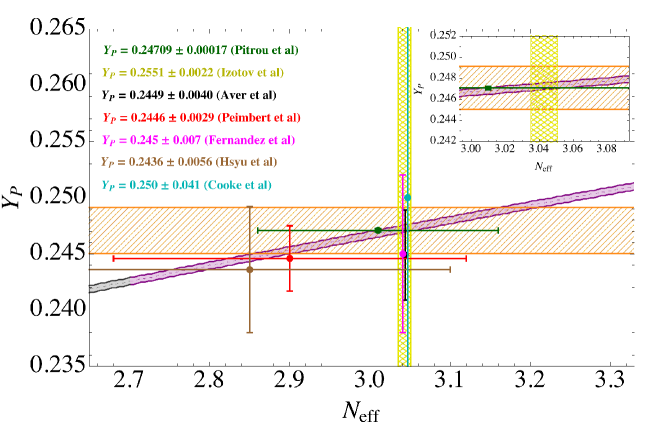
Figure 3: The plot for the predicted primordial Helium abundance $Y_{P}$ as a function of $N_{\rm eff}$. The standard model primordial value $Y_{P}=0.24709\pm 0.00017$ Pitrou:2018cgg at 95% confidence level (CL) is indicated by the green cross. The predicted 95% CL value of $Y_{P}$ with $N_{\rm eff}$ in the Planck range is given by the diagonal band, where the dashed line represents its central value. The gray band in the lower left corner is disfavored by BBN. $N_{\rm eff}$ from the global fit is shown by the vertical hatched region in yellow. The inset at the upper right corner represents the enlarged intersection between the yellow hatched region and the diagonal band in purple. The other crosses are experimental measurements of $Y_{P}$ from different groups as indicated by the legends (see the text for more details).

With the $1\sigma$ bounds for the electroweak vertices and the 4-fermion operators in eqs. (44-46), we randomly varying the dependent Wilson coefficients in eq. (38) inside the 13-dimensional $1\sigma$ sphere with $10^{9}$ points to fit $N_{\rm eff}$ and obtain

$$N_{\rm eff}=3.043\pm 0.008,$$ (49)

which is consistent with the current measurement from Planck Aghanim:2018eyx and the SM prediction Akita:2020szl ; Froustey:2020mcq within $1\sigma$. Note also that the error of $N_{\rm eff}$ in eq. (49) is of the same order as its current theoretical uncertainty. Since the error would be further reduced, for example, at future lepton colliders deBlas:2022ofj , the theoretical uncertainty will become important and shall be included for the study at these next generation experiments. We then make use of AlterBBN Arbey:2018zfh to predict the primordial abundance of helium $Y_{P}$ with $N_{\rm eff}$ being the only free parameter but varying in the Planck range in eq. (42) and by fixing the neutron lifetime $\tau_{n}$ and its uncertainty $\Delta\tau_{n}$ from UCNt:2021pcg . The result is shown in figure 3 by the diagonal band, whose half-width corresponds to the uncertainty in $Y_{P}$. The gray part in the lower-left corner is disfavored by BBN, ignoring the correlation of ${}^{4}{\rm He}$ with the other light elements. The predicted $Y_{P}=0.24709\pm 0.00017$ Pitrou:2018cgg from the SBBN is indicated by the green cross, whose absolute error is given by the vertical bar and is invisible in the plot. The fitted $N_{\rm eff}$ in eq. (49) is then shown by the vertical hatched region in yellow, whose intersection with the diagonal band in purple is shown by the inset in the upper right corner. There, one can clearly see that $N_{\rm eff}$ from the global fit significantly narrows down the space on the $Y_{P}$-$N_{\rm eff}$ plane, corresponding to a significant improvement compared with the diagonal band in the Planck scenario.

Experimentally, $Y_{P}$ can be measured from metal-poor galaxies by observing the ${}^{4}{\rm He}$ and hydrogen emission lines as a function of the galaxy metallicity and extrapolating back to the zero metallicity point for the estimation. In Izotov:2014fga ; Aver:2015iza ; Peimbert:2016bdg ; Fernandez:2018xyz ; Hsyu:2020uqb , they obtained, respectively,

$$Y_{P}=0.2551\pm 0.0022, \,\quad Y_{P}=0.2449\pm 0.0040,\quad Y_{P}=0.2446\pm 0.0029,$$

$$\,Y_{P}=0.245\pm 0.007,\quad Y_{P}=0.2436_{-0.0040}^{+0.0039}.$$ (50)

In addition, from the intergalactic medium, Cooke:2018qzw recently found

$$Y_{P}=0.250_{-0.025}^{+0.033}.$$ (51)

Note that the error in the latter case is much larger than that from metal-poor galaxies. All these experimental results are shown in order in figure 3 as indicated by the legend, with the outlier from Izotov:2014fga beyond the scope of this plot. From this figure, we find all these experimental results also consistent with $N_{\rm eff}$ from the global fit but with large uncertainties.

Recall that the uncertainty in $Y_{P}$ is directly related to that in neutron lifetime Pitrou:2018cgg , we show in figure 3 the uncertainty band of $Y_{P}$ in hatched orange to show explicitly the region insufficient to resolve the $\sim 10\,s$ neutron lifetime anomaly. We stress that, to get this hatched region, we assume the central value of $Y_{P}$ is aligned with the SBBN prediction in Pitrou:2018cgg , and use the central value of $\tau_{n}$ from Pattie:2017vsj ; UCNt:2021pcg as its uncertainty is small below 1 s. Clearly, the SBBN result precludes its possibility in accounting for the difference between the beam and the bottle results, as is well-known. On the other hand, an improvement in extracting $Y_{P}$ from astrophysical observation, reducing the uncertainty in $Y_{P}$ to be within the orange band to be more quantitative, would deepen our understanding on the connection between SBBN and the neutron lifetime anomaly. Here we stress that, at this point, the results in figure 3 are not obtained from the SMEFT global fit except the vertical hatched region in yellow. A full global analysis including all the light elements in the combined framework of SMEFT and SBBN would be desirable, but is beyond the scope of this work since it is more involved and will therefore be investigated in a future work.

5 Conclusions

In light of the percent level precision target of $N_{\rm eff}$ from future cosmological probes like CMB-S4, we think it is now proper to combine the cosmological data together with the collider and the low-energy data sets available to perform a global fit of the SMEFT in searching for new physics indirectly. In this work, by utilizing the $N_{\rm eff}$ data from Planck, as well as its projections for CMB-S4 and CMB-HD, we perform a global fit of the SMEFT without any flavor assumption in the electroweak vertex and (semi-)leptonic 4-fermion sectors. From this work, we find that:

1. In both the flavor universal and the most general flavor scenarios, we find the inclusion of $N_{\rm eff}$ marginally improves the SMEFT global fit due to very small corrections to $N_{\rm eff}$ from the SMEFT operators as seen in eq. (38). The agreement on $N_{\rm eff}$ between the SM prediction and the SMEFT global fit also suggests that the current/planned experimental precision of $N_{\rm eff}$ is very challenging in studying heavy new physics model independently within the SMEFT, rooted in already very stringent constraints on these operators from colliders and low-energy experiments. On the other hand, thanks to these very strong constraints, the $1\sigma$ bound on $N_{\rm eff}$ from the global fit is also significantly reduced and becomes comparable to its current theoretical uncertainty as seen in eq. (49). Since this $1\sigma$ bound would be further reduced at future lepton colliders for example, the theoretical uncertainty in $N_{\rm eff}$ will become important at that stage.

2. $N_{\rm eff}$ from the global fit significantly narrows down the parameter space on the $Y_{P}$-$N_{\rm eff}$ plane compared with that using $N_{\rm eff}$ from Planck, as compared in figure 3. Therefore, improving the experimental precision for both $N_{\rm eff}$ and $Y_{P}$ could add important inputs for a precision test of the SM and the SBBN.

3. By comparing $Y_{P}$ from astrophysical experiments and the global fitted result of $N_{\rm eff}$, we find that improving the experimental precision on $Y_{P}$ from metal-poor galaxies will play an important role in our understanding on the neutron lifetime anomaly within the SBBN, as shown in figure 3.

In the flavor universal case, we commented that the precision in $[\mathcal{O}_{\ell\ell,\ell e,ee}]$ was currently limited by Bhabha scattering at LEP. Looking ahead into the near future, the MOLLER experiment at the Jefferson Laboratory, planned to start data collection in early 2026, will measure the weak mixing angle at a low momentum transfer at the per-mille level. We expect the global fit in this sector to be improved by at least a factor of a few in both the flavor universal and the flavor general cases. Furthermore, in the current work, we only consider $Y_{P}$ by using the global fitted result of $N_{\rm eff}$ and leaving out the other light elements from the consideration of their current uncertainties. It would be desirable to include the full relevant SMEFT operators during BBN for studying $N_{\rm eff}$, the primordial abundances of light elements, and its interplay with the neutron lifetime. This is left for a future work.

Appendix A Analytical expression for $\delta\rho_{\nu}^{\rm tot}/\delta t$ in the SMEFT

Similar to eq. (39), the total neutrino energy density changing rate, ${\delta\rho_{\nu}^{\rm tot}}/{\delta t}\equiv\sum\limits_{\alpha=e}^{\tau}{\delta\rho_{\nu_{\alpha}}}/{\delta t}$ including anti-neutrinos, is given here explicitly:

$$\frac{\delta\rho_{\nu}^{\rm tot}}{\delta t}= \,\frac{8G_{F}^{2}}{\pi^{5}}\left[4\left(8s_{W}^{4}+4s_{W}^{2}+1\right)\left(T_{\gamma}^{9}-T_{\nu_{e}}^{9}\right)+8\left(8s_{W}^{4}-4s_{W}^{2}+1\right)\left(T_{\gamma}^{9}-T_{\nu_{\mu}}^{9}\right)\right.$$

$$\left.\qquad\quad+7T_{\gamma}^{4}\left(\left(8s_{W}^{4}+4s_{W}^{2}+1\right)T_{\nu_{e}}^{4}(T_{\gamma}-T_{\nu_{e}})+2\left(8s_{W}^{4}-4s_{W}^{2}+1\right)T_{\nu_{\mu}}^{4}(T_{\gamma}-T_{\nu_{\mu}})\right)\right.$$

$$\left.\qquad\quad-4[c_{le}]_{1111}s_{W}^{2}\left(4\left(T_{\gamma}^{9}-T_{\nu_{e}}^{9}\right)+7T_{\gamma}^{4}T_{\nu_{e}}^{4}(T_{\gamma}-T_{\nu_{e}})\right)\right.$$

$$\left.\qquad\quad-2[c_{ll}]_{1111}\left(2s_{W}^{2}+1\right)\left(4\left(T_{\gamma}^{9}-T_{\nu_{e}}^{9}\right)+7T_{\gamma}^{4}T_{\nu_{e}}^{4}(T_{\gamma}-T_{\nu_{e}})\right)\right.$$

$$\left.\qquad\quad+4\delta g_{W}^{e\nu}\left(8s_{W}^{4}+4s_{W}^{2}+1\right)\left(4T_{\gamma}^{9}+7T_{\gamma}^{5}T_{\nu_{e}}^{4}-7T_{\gamma}^{4}T_{\nu_{e}}^{5}-4T_{\nu_{e}}^{9}\right)\right.$$

$$\left.\qquad\quad+8\delta g_{Z,L}^{ee}\left(4T_{\gamma}^{9}(4s_{W}^{4}+3s_{W}^{2}-1)-4T_{\nu_{e}}^{9}(4s_{W}^{4}+s_{W}^{2})+(4-8s_{W}^{2})T_{\nu_{\mu}}^{9}\right.\right.$$

$$\left.\left.\qquad\qquad\qquad\qquad+\left(28s_{W}^{4}+7s_{W}^{2}\right)\left(T_{\gamma}^{5}T_{\nu_{e}}^{4}-T_{\gamma}^{4}T_{\nu_{e}}^{5}\right)+\left(7-14s_{W}^{2}\right)\left(T_{\gamma}^{4}T_{\nu_{e}}^{5}-T_{\gamma}^{5}T_{\nu_{e}}^{4}\right)\right)\right.$$

$$\left.\qquad\quad+8\delta g_{Z,R}^{ee}s_{W}^{2}\left(12T_{\gamma}^{9}+7T_{\gamma}^{5}\left(T_{\nu_{e}}^{4}+2T_{\nu_{\mu}}^{4}\right)-7T_{\gamma}^{4}\left(T_{\nu_{e}}^{5}+2T_{\nu_{\mu}}^{5}\right)-4\left(T_{\nu_{e}}^{9}+2T_{\nu_{\mu}}^{9}\right)\right)\right.$$

$$\left.\qquad\quad-4\left([c_{le}]_{2211}+[c_{le}]_{3311}\right)s_{W}^{2}\left(4T_{\gamma}^{9}+7T_{\gamma}^{5}T_{\nu_{\mu}}^{4}-7T_{\gamma}^{4}T_{\nu_{\mu}}^{5}-4T_{\nu_{\mu}}^{9}\right)\right.$$

$$\left.\qquad\quad+2\left([c_{ll}]_{1122}+[c_{ll}]_{1133}\right)\left(1-2s_{W}^{2}\right)\left(4T_{\gamma}^{9}+7T_{\gamma}^{5}T_{\nu_{\mu}}^{4}-7T_{\gamma}^{4}T_{\nu_{\mu}}^{5}-4T_{\nu_{\mu}}^{9}\right)\right.$$

$$\left.\qquad\quad+4\left(\delta g_{W}^{\mu\nu}+\delta g_{W}^{\tau\nu}+\delta g_{Z,L}^{\mu\mu}+\delta g_{Z,L}^{\tau\tau}\right)\left(8s_{W}^{4}-4s_{W}^{2}+1\right)\right.$$

$$\left.\qquad\qquad\times\left(4T_{\gamma}^{9}+7T_{\gamma}^{5}T_{\nu_{\mu}}^{4}-7T_{\gamma}^{4}T_{\nu_{\mu}}^{5}-4T_{\nu_{\mu}}^{9}\right)\right],$$ (52)

where small corrections from non-vanishing $m_{e}$ and Fermi-Dirac statistics are also ignored, and we fix $T_{\nu_{\mu}}=T_{\nu_{\tau}}$ and $\mu_{\nu_{\alpha}}=0$ for simplicity. Clearly, our argument for $\delta n_{\nu}^{\rm tot}/\delta t$ below eq. (39) applies similarly for ${\delta\rho_{\nu}^{\rm tot}}/{\delta t}$. For example, since $s_{W}^{2}\approx 1/4$, the $\delta g_{Z,L}^{ee}$ term also becomes proportional to an overall factor $4s_{W}^{4}+3s_{W}^{2}-1\approx 0$ in the $T_{\nu_{e}}\approx T_{\nu_{\mu}}=T_{\nu_{\tau}}$ limit, explaining why the contribution to $N_{\rm eff}$ from $\delta g_{Z,L}^{ee}$ is relatively small in eq. (38).

References

• (1) ATLAS Collaboration, G.Β Aad etΒ al., Observation of a new particle in the search for the Standard Model Higgs boson with the ATLAS detector at the LHC, Phys. Lett. B 716 (2012) 1–29, [arXiv:1207.7214].
• (2) CMS Collaboration, S.Β Chatrchyan etΒ al., Observation of a New Boson at a Mass of 125 GeV with the CMS Experiment at the LHC, Phys. Lett. B 716 (2012) 30–61, [arXiv:1207.7235].
• (3) S.Β Weinberg, Baryon and Lepton Nonconserving Processes, Phys. Rev. Lett. 43 (1979) 1566–1570.
• (4) W.Β Buchmuller and D.Β Wyler, Effective Lagrangian Analysis of New Interactions and Flavor Conservation, Nucl. Phys. B 268 (1986) 621–653.
• (5) B.Β Grzadkowski, M.Β Iskrzynski, M.Β Misiak, and J.Β Rosiek, Dimension-Six Terms in the Standard Model Lagrangian, JHEP 10 (2010) 085, [arXiv:1008.4884].
• (6) E.Β Fermi, Trends to a Theory of beta Radiation. (In Italian), Nuovo Cim. 11 (1934) 1–19.
• (7) ALEPH, DELPHI, L3, OPAL, LEP Electroweak Collaboration, S.Β Schael etΒ al., Electroweak Measurements in Electron-Positron Collisions at W-Boson-Pair Energies at LEP, Phys. Rept. 532 (2013) 119–244, [arXiv:1302.3415].
• (8) A.Β Efrati, A.Β Falkowski, and Y.Β Soreq, Electroweak constraints on flavorful effective theories, JHEP 07 (2015) 018, [arXiv:1503.07872].
• (9) A.Β Falkowski and K.Β Mimouni, Model independent constraints on four-lepton operators, JHEP 02 (2016) 086, [arXiv:1511.07434].
• (10) L.Β Berthier, M.Β BjΓΈrn, and M.Β Trott, Incorporating doubly resonant $W^{\pm}$ data in a global fit of SMEFT parameters to lift flat directions, JHEP 09 (2016) 157, [arXiv:1606.06693].
• (11) A.Β Falkowski, M.Β GonzΓ‘lez-Alonso, and K.Β Mimouni, Compilation of low-energy constraints on 4-fermion operators in the SMEFT, JHEP 08 (2017) 123, [arXiv:1706.03783].
• (12) T.Β Barklow, K.Β Fujii, S.Β Jung, R.Β Karl, J.Β List, T.Β Ogawa, M.Β E. Peskin, and J.Β Tian, Improved Formalism for Precision Higgs Coupling Fits, Phys. Rev. D 97 (2018), no.Β 5 053003, [arXiv:1708.08912].
• (13) T.Β Barklow, K.Β Fujii, S.Β Jung, M.Β E. Peskin, and J.Β Tian, Model-Independent Determination of the Triple Higgs Coupling at e+e- Colliders, Phys. Rev. D 97 (2018), no.Β 5 053004, [arXiv:1708.09079].
• (14) V.Β Cirigliano, A.Β Falkowski, M.Β GonzΓ‘lez-Alonso, and A.Β RodrΓ­guez-SΓ‘nchez, Hadronic $\tau$ Decays as New Physics Probes in the LHC Era, Phys. Rev. Lett. 122 (2019), no.Β 22 221801, [arXiv:1809.01161].
• (15) J.Β DeΒ Blas, G.Β Durieux, C.Β Grojean, J.Β Gu, and A.Β Paul, On the future of Higgs, electroweak and diboson measurements at lepton colliders, JHEP 12 (2019) 117, [arXiv:1907.04311].
• (16) J.Β Ellis, M.Β Madigan, K.Β Mimasu, V.Β Sanz, and T.Β You, Top, Higgs, Diboson and Electroweak Fit to the Standard Model Effective Field Theory, JHEP 04 (2021) 279, [arXiv:2012.02779].
• (17) J.Β Gu, L.-T. Wang, and C.Β Zhang, Unambiguously Testing Positivity at Lepton Colliders, Phys. Rev. Lett. 129 (2022), no.Β 1 011805, [arXiv:2011.03055].
• (18) SMEFiT Collaboration, J.Β J. Ethier, G.Β Magni, F.Β Maltoni, L.Β Mantani, E.Β R. Nocera, J.Β Rojo, E.Β Slade, E.Β Vryonidou, and C.Β Zhang, Combined SMEFT interpretation of Higgs, diboson, and top quark data from the LHC, JHEP 11 (2021) 089, [arXiv:2105.00006].
• (19) V.Β Cirigliano, D.Β DΓ­az-CalderΓ³n, A.Β Falkowski, M.Β GonzΓ‘lez-Alonso, and A.Β RodrΓ­guez-SΓ‘nchez, Semileptonic tau decays beyond the Standard Model, JHEP 04 (2022) 152, [arXiv:2112.02087].
• (20) G.Β Durieux, A.Β G. Camacho, L.Β Mantani, V.Β Miralles, M.Β M. LΓ³pez, M.Β LlΓ‘cerΒ Moreno, R.Β Poncelet, E.Β Vryonidou, and M.Β Vos, Snowmass White Paper: prospects for the measurement of top-quark couplings, in Snowmass 2021, 5, 2022. arXiv:2205.02140.
• (21) J.Β Ellis, H.-J. He, and R.-Q. Xiao, Probing neutral triple gauge couplings at the LHC and future hadron colliders, Phys. Rev. D 107 (2023), no.Β 3 035005, [arXiv:2206.11676].
• (22) R.Β Aoude, H.Β ElΒ Faham, F.Β Maltoni, and E.Β Vryonidou, Complete SMEFT predictions for four top quark production at hadron colliders, JHEP 10 (2022) 163, [arXiv:2208.04962].
• (23) K.Β Agashe etΒ al., Report of the Topical Group on Top quark physics and heavy flavor production for Snowmass 2021, arXiv:2209.11267.
• (24) V.Β BresΓ³-Pla, A.Β Falkowski, M.Β GonzΓ‘lez-Alonso, and K.Β MonsΓ‘lvez-Pozo, EFT analysis of New Physics at COHERENT, JHEP 05 (2023) 074, [arXiv:2301.07036].
• (25) J.Β Ellis, H.-J. He, and R.-Q. Xiao, Probing Neutral Triple Gauge Couplings with $Z^{*}\gamma\,(\nu\bar{\nu}\gamma)$ Production at Hadron Colliders, arXiv:2308.16887.
• (26) A.Β Dolgov, Neutrinos in cosmology, Phys. Rept. 370 (2002) 333–535, [hep-ph/0202122].
• (27) K.Β Akita and M.Β Yamaguchi, A precision calculation of relic neutrino decoupling, JCAP 08 (2020) 012, [arXiv:2005.07047].
• (28) J.Β Froustey, C.Β Pitrou, and M.Β C. Volpe, Neutrino decoupling including flavour oscillations and primordial nucleosynthesis, JCAP 12 (2020) 015, [arXiv:2008.01074].
• (29) SPT-3G Collaboration, B.Β A. Benson etΒ al., SPT-3G: A Next-Generation Cosmic Microwave Background Polarization Experiment on the South Pole Telescope, Proc. SPIE Int. Soc. Opt. Eng. 9153 (2014) 91531P, [arXiv:1407.2973].
• (30) CMB-S4 Collaboration, K.Β N. Abazajian etΒ al., CMB-S4 Science Book, First Edition, arXiv:1610.02743.
• (31) CORE Collaboration, E.Β DiΒ Valentino etΒ al., Exploring cosmic origins with CORE: Cosmological parameters, JCAP 04 (2018) 017, [arXiv:1612.00021].
• (32) Simons Observatory Collaboration, P.Β Ade etΒ al., The Simons Observatory: Science goals and forecasts, JCAP 02 (2019) 056, [arXiv:1808.07445].
• (33) NASA PICO Collaboration, S.Β Hanany etΒ al., PICO: Probe of Inflation and Cosmic Origins, arXiv:1902.10541.
• (34) N.Β Sehgal etΒ al., CMB-HD: An Ultra-Deep, High-Resolution Millimeter-Wave Survey Over Half the Sky, arXiv:1906.10134.
• (35) CMB-HD Collaboration, S.Β Aiola etΒ al., Snowmass2021 CMB-HD White Paper, arXiv:2203.05728.
• (36) V.Β Shvartsman, Density of relict particles with zero rest mass in the universe, Pisma Zh. Eksp. Teor. Fiz. 9 (1969) 315–317.
• (37) G.Β Steigman, D.Β Schramm, and J.Β Gunn, Cosmological Limits to the Number of Massive Leptons, Phys. Lett. B 66 (1977) 202–204.
• (38) G.Β Mangano, G.Β Miele, S.Β Pastor, and M.Β Peloso, A Precision calculation of the effective number of cosmological neutrinos, Phys. Lett. B 534 (2002) 8–16, [astro-ph/0111408].
• (39) S.Β Hannestad, Oscillation effects on neutrino decoupling in the early universe, Phys. Rev. D 65 (2002) 083006, [astro-ph/0111423].
• (40) A.Β Dolgov, S.Β Hansen, S.Β Pastor, S.Β Petcov, G.Β Raffelt, and D.Β Semikoz, Cosmological bounds on neutrino degeneracy improved by flavor oscillations, Nucl. Phys. B 632 (2002) 363–382, [hep-ph/0201287].
• (41) G.Β Mangano, G.Β Miele, S.Β Pastor, T.Β Pinto, O.Β Pisanti, and P.Β D. Serpico, Relic neutrino decoupling including flavor oscillations, Nucl. Phys. B 729 (2005) 221–234, [hep-ph/0506164].
• (42) P.Β F. deΒ Salas and S.Β Pastor, Relic neutrino decoupling with flavour oscillations revisited, JCAP 07 (2016) 051, [arXiv:1606.06986].
• (43) S.Β Gariazzo, P.Β deΒ Salas, and S.Β Pastor, Thermalisation of sterile neutrinos in the early Universe in the 3+1 scheme with full mixing matrix, JCAP 07 (2019) 014, [arXiv:1905.11290].
• (44) A.Β Heckler, Astrophysical applications of quantum corrections to the equation of state of a plasma, Phys. Rev. D 49 (1994) 611–617.
• (45) N.Β Fornengo, C.Β Kim, and J.Β Song, Finite temperature effects on the neutrino decoupling in the early universe, Phys. Rev. D 56 (1997) 5123–5134, [hep-ph/9702324].
• (46) J.Β J. Bennett, G.Β Buldgen, M.Β Drewes, and Y.Β Y. Wong, Towards a precision calculation of the effective number of neutrinos $N_{\rm eff}$ in the Standard Model I: The QED equation of state, JCAP 03 (2020) 003, [arXiv:1911.04504].
• (47) M.Β EscuderoΒ Abenza, Precision early universe thermodynamics made simple: $N_{\rm eff}$ and neutrino decoupling in the Standard Model and beyond, JCAP 05 (2020) 048, [arXiv:2001.04466].
• (48) Y.Β Du and J.-H. Yu, Neutrino non-standard interactions meet precision measurements of Neff, JHEP 05 (2021) 058, [arXiv:2101.10475].
• (49) J.Β deΒ Blas, Y.Β Du, C.Β Grojean, J.Β Gu, V.Β Miralles, M.Β E. Peskin, J.Β Tian, M.Β Vos, and E.Β Vryonidou, Global SMEFT Fits at Future Colliders, in Snowmass 2021, 6, 2022. arXiv:2206.08326.
• (50) LHC Higgs Cross Section Working Group Collaboration, D.Β deΒ Florian etΒ al., Handbook of LHC Higgs Cross Sections: 4. Deciphering the Nature of the Higgs Sector, arXiv:1610.07922.
• (51) H.Β K. Dreiner, H.Β E. Haber, and S.Β P. Martin, Two-component spinor techniques and Feynman rules for quantum field theory and supersymmetry, Phys. Rept. 494 (2010) 1–196, [arXiv:0812.1594].
• (52) SLAC E158 Collaboration, P.Β L. Anthony etΒ al., Precision measurement of the weak mixing angle in Moller scattering, Phys. Rev. Lett. 95 (2005) 081601, [hep-ex/0504049].
• (53) MOLLER Collaboration, J.Β Benesch etΒ al., The MOLLER Experiment: An Ultra-Precise Measurement of the Weak Mixing Angle Using M\oller Scattering, arXiv:1411.4088.
• (54) F.Β Reines, H.Β S. Gurr, and H.Β W. Sobel, Detection of anti-electron-neutrino e Scattering, Phys. Rev. Lett. 37 (1976) 315–318.
• (55) R.Β C. Allen etΒ al., Study of electron-neutrino electron elastic scattering at LAMPF, Phys. Rev. D 47 (1993) 11–28.
• (56) CHARM-II Collaboration, P.Β Vilain etΒ al., Experimental study of electromagnetic properties of the muon-neutrino in neutrino - electron scattering, Phys. Lett. B 345 (1995) 115–118.
• (57) CHARM-II Collaboration, P.Β Vilain etΒ al., A Precise measurement of the cross-section of the inverse muon decay muon-neutrino + e- –$>$ mu- + electron-neutrino, Phys. Lett. B 364 (1995) 121–126.
• (58) LSND Collaboration, L.Β B. Auerbach etΒ al., Measurement of electron - neutrino - electron elastic scattering, Phys. Rev. D 63 (2001) 112001, [hep-ex/0101039].
• (59) TEXONO Collaboration, M.Β Deniz etΒ al., Constraints on Non-Standard Neutrino Interactions and Unparticle Physics with Neutrino-Electron Scattering at the Kuo-Sheng Nuclear Power Reactor, Phys. Rev. D 82 (2010) 033004, [arXiv:1006.1947].
• (60) J.Β A. Formaggio and G.Β P. Zeller, From eV to EeV: Neutrino Cross Sections Across Energy Scales, Rev. Mod. Phys. 84 (2012) 1307–1341, [arXiv:1305.7513].
• (61) Planck Collaboration, N.Β Aghanim etΒ al., Planck 2018 results. VI. Cosmological parameters, Astron. Astrophys. 641 (2020) A6, [arXiv:1807.06209].
• (62) C.Β M. Ankenbrandt etΒ al., Status of muon collider research and development and future plans, Phys. Rev. ST Accel. Beams 2 (1999) 081001, [physics/9901022].
• (63) M.Β Forslund and P.Β Meade, High precision higgs from high energy muon colliders, JHEP 08 (2022) 185, [arXiv:2203.09425].
• (64) J.Β deΒ Blas, J.Β Gu, and Z.Β Liu, Higgs boson precision measurements at a 125Β GeV muon collider, Phys. Rev. D 106 (2022), no.Β 7 073007, [arXiv:2203.04324].
• (65) CMS Collaboration, A.Β Tumasyan etΒ al., Search for Higgs boson pairs decaying to WW*WW*, WW*$\tau\tau$, and $\tau\tau\tau\tau$ in proton-proton collisions at $\sqrt{s}$ = 13 TeV, JHEP 07 (2023) 095, [arXiv:2206.10268].
• (66) ALEPH, DELPHI, L3, OPAL, SLD, LEP Electroweak Working Group, SLD Electroweak Group, SLD Heavy Flavour Group Collaboration, S.Β Schael etΒ al., Precision electroweak measurements on the $Z$ resonance, Phys. Rept. 427 (2006) 257–454, [hep-ex/0509008].
• (67) https://moller.jlab.org/moller_root/.
• (68) https://www.umass.edu/physics/news/2022-11-22-moller-project-funded.
• (69) CLIC Physics Working Group Collaboration, E.Β Accomando etΒ al., Physics at the CLIC multi-TeV linear collider, in 11th International Conference on Hadron Spectroscopy, CERN Yellow Reports: Monographs, 6, 2004. hep-ph/0412251.
• (70) A.Β Robson and P.Β Roloff, Updated CLIC luminosity staging baseline and Higgs coupling prospects, arXiv:1812.01644.
• (71) ILC Collaboration, The International Linear Collider Technical Design Report - Volume 2: Physics, arXiv:1306.6352.
• (72) ILC International Development Team Collaboration, A.Β Aryshev etΒ al., The International Linear Collider: Report to Snowmass 2021, arXiv:2203.07622.
• (73) CEPC Study Group Collaboration, M.Β Dong etΒ al., CEPC Conceptual Design Report: Volume 2 - Physics & Detector, arXiv:1811.10545.
• (74) CEPC Physics Study Group Collaboration, H.Β Cheng etΒ al., The Physics potential of the CEPC. Prepared for the US Snowmass Community Planning Exercise (Snowmass 2021), in Snowmass 2021, 5, 2022. arXiv:2205.08553.
• (75) FCC Collaboration, A.Β Abada etΒ al., FCC-ee: The Lepton Collider: Future Circular Collider Conceptual Design Report Volume 2, Eur. Phys. J. ST 228 (2019), no.Β 2 261–623.
• (76) G.Β Bernardi etΒ al., The Future Circular Collider: a Summary for the US 2021 Snowmass Process, arXiv:2203.06520.
• (77) M.Β GonzΓ‘lez-Alonso and J.Β MartinΒ Camalich, Global Effective-Field-Theory analysis of New-Physics effects in (semi)leptonic kaon decays, JHEP 12 (2016) 052, [arXiv:1605.07114].
• (78) Particle Data Group Collaboration, R.Β L. Workman etΒ al., Review of Particle Physics, PTEP 2022 (2022) 083C01.
• (79) N.Β Cabibbo, Unitary Symmetry and Leptonic Decays, Phys. Rev. Lett. 10 (1963) 531–533.
• (80) M.Β Kobayashi and T.Β Maskawa, CP Violation in the Renormalizable Theory of Weak Interaction, Prog. Theor. Phys. 49 (1973) 652–657.
• (81) A.Β Sirlin, Current Algebra Formulation of Radiative Corrections in Gauge Theories and the Universality of the Weak Interactions, Rev. Mod. Phys. 50 (1978) 573. [Erratum: Rev.Mod.Phys. 50, 905 (1978)].
• (82) W.Β J. Marciano and A.Β Sirlin, Improved calculation of electroweak radiative corrections and the value of V(ud), Phys. Rev. Lett. 96 (2006) 032002, [hep-ph/0510099].
• (83) C.-Y. Seng, M.Β Gorchtein, H.Β H. Patel, and M.Β J. Ramsey-Musolf, Reduced Hadronic Uncertainty in the Determination of $V_{ud}$, Phys. Rev. Lett. 121 (2018), no.Β 24 241804, [arXiv:1807.10197].
• (84) A.Β T. Yue, M.Β S. Dewey, D.Β M. Gilliam, G.Β L. Greene, A.Β B. Laptev, J.Β S. Nico, W.Β M. Snow, and F.Β E. Wietfeldt, Improved Determination of the Neutron Lifetime, Phys. Rev. Lett. 111 (2013), no.Β 22 222501, [arXiv:1309.2623].
• (85) R.Β W. Pattie, Jr. etΒ al., Measurement of the neutron lifetime using a magneto-gravitational trap and in situ detection, Science 360 (2018), no.Β 6389 627–632, [arXiv:1707.01817].
• (86) UCN$\tau$ Collaboration, F.Β M. Gonzalez etΒ al., Improved neutron lifetime measurement with UCN$\tau$, Phys. Rev. Lett. 127 (2021), no.Β 16 162501, [arXiv:2106.10375].
• (87) F.Β E. Wietfeldt and G.Β L. Greene, Colloquium: The neutron lifetime, Rev. Mod. Phys. 83 (2011), no.Β 4 1173–1192.
• (88) B.Β Fornal and B.Β Grinstein, Dark Matter Interpretation of the Neutron Decay Anomaly, Phys. Rev. Lett. 120 (2018), no.Β 19 191801, [arXiv:1801.01124]. [Erratum: Phys.Rev.Lett. 124, 219901 (2020)].
• (89) A.Β Czarnecki, W.Β J. Marciano, and A.Β Sirlin, Neutron Lifetime and Axial Coupling Connection, Phys. Rev. Lett. 120 (2018), no.Β 20 202002, [arXiv:1802.01804].
• (90) D.Β Dubbers, H.Β Saul, B.Β MΓ€rkisch, T.Β Soldner, and H.Β Abele, Exotic decay channels are not the cause of the neutron lifetime anomaly, Phys. Lett. B 791 (2019) 6–10, [arXiv:1812.00626].
• (91) C.Β Pitrou, A.Β Coc, J.-P. Uzan, and E.Β Vangioni, Precision big bang nucleosynthesis with improved Helium-4 predictions, Phys. Rept. 754 (2018) 1–66, [arXiv:1801.08023].
• (92) A.Β Arbey, J.Β Auffinger, K.Β P. Hickerson, and E.Β S. Jenssen, AlterBBN v2: A public code for calculating Big-Bang nucleosynthesis constraints in alternative cosmologies, Comput. Phys. Commun. 248 (2020) 106982, [arXiv:1806.11095].
• (93) Y.Β I. Izotov, T.Β X. Thuan, and N.Β G. Guseva, A new determination of the primordial He abundance using the He i $\lambda$10830 Γ… emission line: cosmological implications, Mon. Not. Roy. Astron. Soc. 445 (2014), no.Β 1 778–793, [arXiv:1408.6953].
• (94) E.Β Aver, K.Β A. Olive, and E.Β D. Skillman, The effects of He I $\lambda$10830 on helium abundance determinations, JCAP 07 (2015) 011, [arXiv:1503.08146].
• (95) A.Β Peimbert, M.Β Peimbert, and V.Β Luridiana, The primordial helium abundance and the number of neutrino families, Rev. Mex. Astron. Astrofis. 52 (2016), no.Β 2 419–424, [arXiv:1608.02062].
• (96) V.Β FernΓ‘ndez, E.Β Terlevich, A.Β I. DΓ­az, R.Β Terlevich, and F.Β F. Rosales-Ortega, Primordial helium abundance determination using sulphur as metallicity tracer, Monthly Notices of the Royal Astronomical Society 478 (05, 2018) 5301–5319, [arXiv:1804.10701].
• (97) T.Β Hsyu, R.Β J. Cooke, J.Β X. Prochaska, and M.Β Bolte, The PHLEK Survey: A New Determination of the Primordial Helium Abundance, Astrophys. J. 896 (2020), no.Β 1 77, [arXiv:2005.12290].
• (98) R.Β Cooke and M.Β Fumagalli, Measurement of the primordial helium abundance from the intergalactic medium, Nature Astron. 2 (2018), no.Β 12, 957–961, [arXiv:1810.06561].
• (99) A.Β G. Polnarev and M.Β Y. Khlopov, The ERA of superheavy-particle dominance and big bang nucleosynthesis, Astron. Zh. 59 (1982) 15–19 [English translation: Sov. Astron. (1982) V. 26, 9–12].
• (100) A.Β G. Doroshkevich and M.Β Y. Khlopov, Grand Unification Cosmology and the Parameters of a Neutrino Dominated Universe, Astron. Zh. 9 (1983) 323–326 [English translation: Sov. Astron. Lett. (1983) V. 9, no.3, 171–173].
• (101) A.Β G. Doroshkevich and M.Β Y. Khlopov, On the physical nature of dark matter of the Universe, Yadernaya Fizika 39 (1984) 869–870 [English translation: Sov.J.Nucl.Phys. (1984) V.39, 551–553].
• (102) A.Β G. Doroshkevich and M.Β Y. Khlopov, Formation of structure in the Universe with unstable neutrinos, Mon. Not. Roy. astr. Soc. 211 (1984) 279–282.
• (103) A.Β G. Doroshkevich and M.Β Y. Khlopov, Fluctuations of the Cosmic Background Temperature in Unstable-Particle Cosmologies, Astron. Zh. 11 (1985) 563–568 [English translation: Sov. Astronomy Lett. (1985) V.11, no.4, 236–238].
• (104) A.Β G. Doroshkevich, A.Β A. Klypin, and M.Β Y. Khlopov, Cosmological Models with Unstable Neutrinos, Astron. Zh. 65 (1988) 248–262 [English translation: Sov. Astron. (1988), V. 32, no.2, 127].
• (105) A.Β G. Doroshkevich, M.Β Y. Khlopov, and A.Β A. Klypin, Large-scale structure formation by decaying massive neutrinos, Mon.Not.Roy.astr.soc. 239 (1989) 923–938.
• (106) M.Β Y. Khlopov, Physical arguments, favouring multicomponent dark matter. In: Dark matter in cosmology, clocks and tests of fundamental laws, Eds.B.Guiderdoni et al., Editions Frontieres (1989) 133–138.
• (107) Z.Β G. Berezhiani and M.Β Y. Khlopov, Physics of cosmological dark matter in the theory of broken family symmetry, Yadernaya Fizika 52 (1990) 96–103 [English translation: Sov.J.Nucl.Phys. (1990) V.52, PP.60–64].
• (108) Z.Β G. Berezhiani and M.Β Y. Khlopov, Cosmology of spontaneously broken gauge family symmetry with axion solution of strong CP-problem, Z.Phys.C- Particles and Fields 49 (1991) 73–78.
• (109) A.Β S. Sakharov and M.Β Y. Khlopov, Horizontal unification as the phenomenology of the theory of everything, Yadernaya Fizika 57 (1994) 690–697 [English translation: Phys.Atom.Nucl. (1994) V. 57, PP. 651–658].
• (110) M.Β Khlopov, Fundamental Particle Structure in the Cosmological Dark Matter, Int. J. Mod. Phys. A 28 (2013) 1330042, [arXiv:1311.2468].
• (111) S.Β Deng and L.Β Bian, Constraints on new physics around the MeV scale with cosmological observations, Phys. Rev. D 108 (2023), no.Β 6 063516, [arXiv:2304.06576].