Passivity and Decentralized Stability Conditions for Grid-Forming Converters

Xiuqiang He,  and Florian Dörfler,  This work was supported by the European Union’s Horizon 2020 research and innovation program under Grant 883985.The authors are with the Automatic Control Laboratory, ETH Zurich, 8092 Zurich, Switzerland. Email:{xiuqhe,dorfler}@ethz.ch.
Abstract

We prove that the popular grid-forming control, i.e., dispatchable virtual oscillator control (dVOC), also termed complex droop control, exhibits output-feedback passivity in its large-signal model, featuring an explicit and physically meaningful passivity index. Using this passivity property, we derive decentralized stability conditions for the transient stability of dVOC in multi-converter grid-connected systems, beyond prior small-signal stability results. The decentralized conditions are of practical significance, particularly for ensuring the transient stability of renewable power plants under grid disturbances.

Index Terms:
Complex droop control, dispatchable virtual oscillator control, grid-forming control, passivity, transient stability.

I Introduction

Renewable energy sources are being ever-increasingly integrated into power grids. Grid-forming control technologies are emerging in power systems to maintain system strength and stability. Unlike large-capacity synchronous generators, renewable power generation features a substantial number of small-capacity generating units connected to power grids. Conventional stability analysis faces growing difficulties when applied to investigate numerous renewable power generating units in a centralized manner. These challenges stem from both analytical intractability and computational burdens due to numerous generating units as well as confidentiality restrictions on system-wide data or model availability [1]. Additionally, since grid-forming converters operate autonomously, and exhibit rich and varied dynamic behavior, aggregated equivalent modeling and analysis [2] is rarely applicable.

Decentralized stability analysis has drawn increasing attention in recent years [3, 4, 5]. Decentralized approaches divide nodes and networks, treating each node’s dynamics and the network coupling separately, relying solely on local and essential network data. Passivity serves as a fundamental tool in decentralized stability analysis, applicable to both nonlinear and linearized systems [6] (roughly corresponding to transient stability and small-signal stability analysis in power systems). There have been many studies exploring passivity-based conditions for small-signal stability of linearized converter systems [3, 4]. However, the area of decentralized stability analysis for large-signal transient stability remains underexplored [1]. In [5], decentralized stability conditions for nonlinear dynamics of synchronous generators and classical grid-forming controls are established, ensuring the local stability of a given equilibrium point and corresponding controller setpoints.

We examine the passivity and decentralized stability conditions for the most recent grid-forming control, dispatchable virtual oscillator control (dVOC), also called complex droop control [7]. Our results feature large-signal passivity analysis for global asymptotic stability, which, to the best of our knowledge, cannot or can hardly be achieved through classical grid-forming controls. We reveal that dVOC-controlled multi-converter grid-connected systems, satisfying our prescribed decentralized conditions, achieve large-signal/transient stability.

II System Model With Feedback Connection

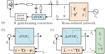
Grid-forming converters measure their output currents and establish the terminal voltages, as depicted in Fig. 1(a). In our modeling and analysis, a three-phase balanced condition is considered, and the grid synchronous reference frame is employed [3] since the system’s steady state converges to the grid frequency. In the grid reference frame, the converter voltage and the output current are expressed with $dq$-axis components as $\underline{v}_{k}\coloneqq v_{{\rm d},k}+jv_{{\rm q},k}$ and $\underline{i}_{k}\coloneqq i_{{\rm d},k}+ji_{{\rm q},k}$, respectively. We use underlines throughout to indicate complex variables.

Refer to caption
Figure 1: (a) Multi-converter grid-connected systems with dVOC grid-forming control. (b) System model with feedback connection. (c) In incremental form w.r.t to equilibria, the passivity index of the dVOC-controlled node dynamics is denoted as $\delta_{k}$ while the passivity index of the (rotated) network is denoted as $\varepsilon_{\rm net}$, establishing decentralized stability conditions as $\delta_{k}+\varepsilon_{\rm net}>0,\forall k$.

1) Grid-Forming Dynamics: After transformed into the grid reference frame, the dVOC grid-forming voltage dynamics in complex-voltage coordinates are given as [7]

$$\dot{\underline{v}}_{k}=j\omega_{\Delta}\underline{v}_{k}+\eta_{k}e^{j\varphi}\bigl{(}\tfrac{p_{k}^{\star}-jq_{k}^{\star}}{v_{k}^{\star 2}}\underline{v}_{k}-\underline{i}_{k}\bigr{)}+\eta_{k}\alpha_{k}\tfrac{v_{k}^{\star 2}-|\underline{v}_{k}|^{2}}{v_{k}^{\star 2}}\underline{v}_{k},$$ (1)

with gains $\eta_{k}\in\mathbb{R}_{>0}$, $\alpha_{k}\in\mathbb{R}_{>0}$, and grid frequency deviation $\omega_{\Delta}\coloneqq\omega_{0}-\omega_{\rm g}$. The angle ${\varphi}\in[0,\pi/2]$ is chosen typically as the network impedance angle, and $p_{k}^{\star}$, $q_{k}^{\star}$, and $v_{k}^{\star}$ are the setpoints for active power, reactive power, and voltage amplitude, respectively. In (1), the first term $j\omega_{0}\underline{v}_{k}$ (before rotation) stands for an oscillator at $\omega_{0}$, the second term synchronizes the relative phases to track the power setpoints via current feedback, and the third term regulates the voltage amplitude.

2) Network Representation: For the set of $N$ converters, we denote $\underline{\boldsymbol{v}}\coloneqq[\underline{v}_{1},\cdots,\underline{v}_{N}]^{\mathsf{T}}$ and $\underline{\boldsymbol{i}}\coloneqq[\underline{i}_{1},\cdots,\underline{i}_{N}]^{\mathsf{T}}$. Consider that the network electromagnetic dynamics and the converter inner-loop dynamics are sufficiently fast such that the dVOC dynamics do not interfere with these dynamics. Under this assumption, we consider a static network representation as

$$\underline{\boldsymbol{i}}=\underline{\boldsymbol{Y}}\,\underline{\boldsymbol{v}}-\underline{\boldsymbol{y}}v_{\rm g},$$ (2)

where $v_{\rm g}$ is the grid voltage, and the admittance matrix $\underline{\boldsymbol{Y}}$ and vector $\underline{\boldsymbol{y}}$ can be obtained from Kron reduction, where the intermediate nodes in the network are eliminated, see Fig. 1(a). If a virtual impedance is used for current limiting during grid faults [8], it should also be included in (2).

3) System Model With Feedback Connection: We synthesize the node dynamics in (1) and the network equation in (2) to establish the closed-loop feedback system, as shown in Fig. 1(b). We further define an equivalent system, where the network admittance is rotated by $\varphi$, i.e., the angle employed in dVOC. This equivalent system proves to be more tractable in passivity analysis, and this rotation transformation is also consistent with the typical $p$-$q$ frame transformation in grid-forming feedback controls concerning inductive-resistive networks [9]. To do so, we define rotated current as $\underline{i}_{\varphi,k}\coloneqq e^{j\varphi}\underline{i}_{k}$ and $\underline{\boldsymbol{i}}_{\varphi}\coloneqq e^{j\varphi}\underline{\boldsymbol{i}}$. The node dynamics in (1) and the network equation in (2) are represented equivalently as

$\displaystyle\dot{\underline{v}}_{k}$ $\displaystyle=\eta_{k}\bigl{[}\tfrac{j\omega_{\Delta}}{\eta_{k}}\underline{v}_{k}+(\sigma_{\varphi,k}^{\star}+j\rho_{\varphi,k}^{\star})\underline{v}_{k}-\underline{i}_{\varphi,k}+\alpha_{k}\tfrac{v_{k}^{\star 2}-|\underline{v}_{k}|^{2}}{v_{k}^{\star 2}}\underline{v}_{k}\bigr{]},$ (3)
$\displaystyle\underline{\boldsymbol{i}}_{\varphi}$ $\displaystyle=e^{j\varphi}\underline{\boldsymbol{Y}}\,\underline{\boldsymbol{v}}-e^{j\varphi}\underline{\boldsymbol{y}}v_{\rm g}.$ (4)

where $\sigma_{\varphi,k}^{\star}+j\rho_{\varphi,k}^{\star}\coloneqq e^{j\varphi}\tfrac{p_{k}^{\star}-jq_{k}^{\star}}{v_{k}^{\star 2}}$. We define steady-state voltages and currents with a subscript $\rm s$ as $\underline{\boldsymbol{v}}_{\rm s}=[\underline{v}_{{\rm s},1},\cdots,\underline{v}_{{\rm s},N}]^{\mathsf{T}}$, $\underline{\boldsymbol{i}}_{\varphi{\rm s}}=[\underline{i}_{\varphi{\rm s},1},\cdots,\underline{i}_{\varphi{\rm s},N}]^{\mathsf{T}}$, and increment variables w.r.t the steady state as $\tilde{\underline{\boldsymbol{v}}}\coloneqq\underline{\boldsymbol{v}}-\underline{\boldsymbol{v}}_{\rm s}$ and $\tilde{\underline{\boldsymbol{i}}}_{\varphi}\coloneqq\underline{\boldsymbol{i}}_{\varphi}-\underline{\boldsymbol{i}}_{\varphi{\rm s}}$.

III Passivity and Stability Results

We first recall the definition of passivity. The system $\dot{\boldsymbol{x}}=\boldsymbol{f}(\boldsymbol{x},\boldsymbol{u})$, $\boldsymbol{y}=\boldsymbol{h}(\boldsymbol{x},\boldsymbol{u})$ is said to be output-feedback passive if there exists a positive semidefinite storage function $V(\boldsymbol{x})$ such that $\boldsymbol{u}^{\mathsf{T}}\boldsymbol{y}\geq\dot{V}+\boldsymbol{y}^{\mathsf{T}}\boldsymbol{\rho}(\boldsymbol{y})$ for some function $\boldsymbol{\rho}$ [6, Def. 6.3]. Moreover, it is said to be input-feedforward passive if $\boldsymbol{u}^{\mathsf{T}}\boldsymbol{y}\geq\dot{V}+\boldsymbol{u}^{\mathsf{T}}\boldsymbol{\varphi}(\boldsymbol{u})$ for some function $\boldsymbol{\varphi}$ [6, Def. 6.1]. If there exits $\boldsymbol{\rho}(\boldsymbol{y})=\delta\boldsymbol{y}$ for some $\delta\in\mathbb{R}$ or $\boldsymbol{\varphi}(\boldsymbol{u})=\varepsilon\boldsymbol{u}$ for some $\varepsilon\in\mathbb{R}$, we refer $\delta$ or $\varepsilon$ to as the passivity index.

III-A Passivity Index of Grid-Forming Dynamics

Proposition 1.

The dVOC dynamics in (3), with input $-\underline{i}_{\varphi,k}$ and output $\underline{v}_{k}$, are output-feedback passive w.r.t an equilibrium $\underline{v}_{{\rm s},k}$, where the passivity index is given as

δkRe{ejφpkjqkvk2}αk+αk12vk2|v¯s,k|2.subscript𝛿𝑘superscript𝑒𝑗𝜑superscriptsubscript𝑝𝑘𝑗superscriptsubscript𝑞𝑘superscriptsubscript𝑣𝑘absent2subscript𝛼𝑘subscript𝛼𝑘12superscriptsubscript𝑣𝑘absent2superscriptsubscript¯𝑣s𝑘2\delta_{k}\coloneqq-\real\{e^{j\varphi}\tfrac{p_{k}^{\star}-jq_{k}^{\star}}{v_{k}^{\star 2}}\bigr{\}}-\alpha_{k}+\alpha_{k}\tfrac{1}{2v_{k}^{\star 2}}|\underline{v}_{{\rm s},k}|^{2}. (5)
{proof}

A positive-definite storage function is defined as

$$V_{k}\coloneqq\tfrac{1}{2\eta_{k}}(\overline{\underline{v}}_{k}-\overline{\underline{v}}_{{\rm s},k})(\underline{v}_{k}-\underline{v}_{{\rm s},k}),$$

where $\overline{\underline{v}}_{k}$ and $\overline{\underline{v}}_{{\rm s},k}$ are the complex conjugate of $\underline{v}_{k}$ and $\underline{v}_{{\rm s},k}$, respectively (overlines indicate complex conjugate), and $\underline{v}_{{\rm s},k}$ satisfies the steady-state relationship of (3) as

$$\underline{i}_{\varphi{\rm s},k}=\tfrac{j\omega_{\Delta}}{\eta_{k}}\underline{v}_{{\rm s},k}+(\sigma_{\varphi,k}^{\star}+j\rho_{\varphi,k}^{\star})\underline{v}_{{\rm s},k}+\alpha_{k}\tfrac{v_{k}^{\star 2}-|\underline{v}_{{\rm s},k}|^{2}}{v_{k}^{\star 2}}\underline{v}_{{\rm s},k}.$$ (6)

The time derivative of $V_{k}$ along the node dynamics in (3) is V˙k=12ηk(v¯¯kv¯¯s,k)v¯˙k+12ηkv¯¯˙k(v¯kv¯s,k)=1ηkRe{(v¯¯kv¯¯s,k)v¯˙k}=Re{(v¯¯kv¯¯s,k)[jωΔηkv¯k+(σφ,k+jρφ,k)v¯ki¯φs,k+αkvk2|v¯k|2vk2v¯k]}+Re{(v¯¯kv¯¯s,k)(i¯φs,ki¯φ,k)}subscript˙𝑉𝑘12subscript𝜂𝑘subscript¯¯𝑣𝑘subscript¯¯𝑣s𝑘subscript˙¯𝑣𝑘12subscript𝜂𝑘subscript˙¯¯𝑣𝑘subscript¯𝑣𝑘subscript¯𝑣s𝑘1subscript𝜂𝑘subscript¯¯𝑣𝑘subscript¯¯𝑣s𝑘subscript˙¯𝑣𝑘subscript¯¯𝑣𝑘subscript¯¯𝑣s𝑘delimited-[]𝑗subscript𝜔Δsubscript𝜂𝑘subscript¯𝑣𝑘superscriptsubscript𝜎𝜑𝑘𝑗superscriptsubscript𝜌𝜑𝑘subscript¯𝑣𝑘subscript¯𝑖𝜑s𝑘subscript𝛼𝑘superscriptsubscript𝑣𝑘absent2superscriptsubscript¯𝑣𝑘2superscriptsubscript𝑣𝑘absent2subscript¯𝑣𝑘subscript¯¯𝑣𝑘subscript¯¯𝑣s𝑘subscript¯𝑖𝜑s𝑘subscript¯𝑖𝜑𝑘{\dot{V}}_{k}=\tfrac{1}{2\eta_{k}}(\overline{\underline{v}}_{k}-\overline{\underline{v}}_{{\rm s},k})\dot{\underline{v}}_{k}+\tfrac{1}{2\eta_{k}}\dot{\overline{\underline{v}}}_{k}(\underline{v}_{k}-\underline{v}_{{\rm s},k})=\tfrac{1}{\eta_{k}}\real\{(\overline{\underline{v}}_{k}-\overline{\underline{v}}_{{\rm s},k})\dot{\underline{v}}_{k}\}=\real\{(\overline{\underline{v}}_{k}-\overline{\underline{v}}_{{\rm s},k})\bigl{[}\tfrac{j\omega_{\Delta}}{\eta_{k}}\underline{v}_{k}+(\sigma_{\varphi,k}^{\star}+j\rho_{\varphi,k}^{\star})\underline{v}_{k}-\underline{i}_{\varphi{\rm s},k}+\alpha_{k}\tfrac{v_{k}^{\star 2}-|\underline{v}_{k}|^{2}}{v_{k}^{\star 2}}{\underline{v}_{k}}\bigr{]}\bigr{\}}+\real\{(\overline{\underline{v}}_{k}-\overline{\underline{v}}_{{\rm s},k})(\underline{i}_{\varphi{\rm s},k}-\underline{i}_{\varphi,k})\}. By applying (6), we obtain that V˙k=(σφ,k+αk)|v¯kv¯s,k|2αk1vk2Re{(v¯¯kv¯¯s,k)(|v¯k|2v¯k|v¯s,k|2v¯s,k)}+Re{(v¯¯kv¯¯s,k)(i¯φs,ki¯φ,k)}subscript˙𝑉𝑘superscriptsubscript𝜎𝜑𝑘subscript𝛼𝑘superscriptsubscript¯𝑣𝑘subscript¯𝑣s𝑘2subscript𝛼𝑘1superscriptsubscript𝑣𝑘absent2subscript¯¯𝑣𝑘subscript¯¯𝑣s𝑘superscriptsubscript¯𝑣𝑘2subscript¯𝑣𝑘superscriptsubscript¯𝑣s𝑘2subscript¯𝑣s𝑘subscript¯¯𝑣𝑘subscript¯¯𝑣s𝑘subscript¯𝑖𝜑s𝑘subscript¯𝑖𝜑𝑘{\dot{V}}_{k}=(\sigma_{\varphi,k}^{\star}+\alpha_{k})|{\underline{v}_{k}-\underline{v}_{{\rm s},k}}|^{2}-\alpha_{k}\tfrac{1}{v_{k}^{\star 2}}\real\{(\overline{\underline{v}}_{k}-\overline{\underline{v}}_{{\rm s},k})(|\underline{v}_{k}|^{2}\underline{v}_{k}-|\underline{v}_{{\rm s},k}|^{2}\underline{v}_{{\rm s},k})\bigr{\}}+\real\{(\overline{\underline{v}}_{k}-\overline{\underline{v}}_{{\rm s},k})(\underline{i}_{\varphi{\rm s},k}-\underline{i}_{\varphi,k})\}. We bound the second term as Re{(v¯¯kv¯¯s,k)(|v¯k|2v¯k|v¯s,k|2v¯s,k)}12|v¯s,k|2|v¯kv¯s,k|2subscript¯¯𝑣𝑘subscript¯¯𝑣s𝑘superscriptsubscript¯𝑣𝑘2subscript¯𝑣𝑘superscriptsubscript¯𝑣s𝑘2subscript¯𝑣s𝑘12superscriptsubscript¯𝑣s𝑘2superscriptsubscript¯𝑣𝑘subscript¯𝑣s𝑘2\real\{(\overline{\underline{v}}_{k}-\overline{\underline{v}}_{{\rm s},k})(|\underline{v}_{k}|^{2}\underline{v}_{k}-|\underline{v}_{{\rm s},k}|^{2}\underline{v}_{{\rm s},k})\bigr{\}}\geq\tfrac{1}{2}|\underline{v}_{{\rm s},k}|^{2}|\underline{v}_{k}-\underline{v}_{{\rm s},k}|^{2}, which holds due to $(\boldsymbol{x}-\boldsymbol{y})^{\mathsf{T}}(\norm{\boldsymbol{x}}^{2}\boldsymbol{x}-\norm{\boldsymbol{y}}^{2}\boldsymbol{y})\geq\tfrac{1}{2}\norm{\boldsymbol{y}}^{2}\norm{\boldsymbol{x}-\boldsymbol{y}}^{2}$, $\forall\boldsymbol{x},\boldsymbol{y}\in\mathbb{R}^{2}$ [7, Proposition 6], in real variable form. Therefore,

$\displaystyle{\dot{V}}_{k}$ $\displaystyle\leq(\sigma_{\varphi,k}^{\star}+\alpha_{k}-\alpha_{k}\tfrac{1}{2v_{k}^{\star 2}}|\underline{v}_{{\rm s},k}|^{2})|\underline{v}_{k}-\underline{v}_{{\rm s},k}|^{2}$ (7)
+Re{(v¯¯kv¯¯s,k)(i¯φs,ki¯φ,k)},subscript¯¯𝑣𝑘subscript¯¯𝑣s𝑘subscript¯𝑖𝜑s𝑘subscript¯𝑖𝜑𝑘\displaystyle\quad\ +\real\{(\overline{\underline{v}}_{k}-\overline{\underline{v}}_{{\rm s},k})(\underline{i}_{\varphi{\rm s},k}-\underline{i}_{\varphi,k})\},

which indicates that the node dynamics with incremental input $\underline{u}_{k}\coloneqq-(\underline{i}_{\varphi,k}-\underline{i}_{\varphi{\rm s},k})$ and output $\underline{y}_{k}\coloneqq(\underline{v}_{k}-\underline{v}_{{\rm s},k})$ is output-feedback passive, as in the standard real-variable form $\boldsymbol{u}^{\mathsf{T}}\boldsymbol{y}\geq\dot{V}+\delta_{k}\boldsymbol{y}^{\mathsf{T}}\boldsymbol{y}$, where $\delta_{k}=-(\sigma_{\varphi,k}^{\star}+\alpha_{k}-\alpha_{k}\tfrac{1}{2v_{k}^{\star 2}}|\underline{v}_{{\rm s},k}|^{2})$ is identified as the node passivity index.

Remark 1.

The inequality (7) physically means that the power flowing into the converter is greater than the rate of change of the energy storage in the controller together with the excess or shortage of passivity represented by the passivity index. The passivity index is also physically meaningful in the sense that it relates the passivity excess ($\delta_{k}>0$) or shortage ($\delta_{k}<0$) to the controller setpoints, gains, and steady-state voltage levels. Typically, $\delta_{k}<0$ occurs since $\alpha>0$. High power setpoints are detrimental to passivity while high voltage levels promote passivity, which is in line with engineering experience. Moreover, we can omit the last term of $\delta_{k}$, making the passivity evaluation independent of the equilibrium point information $|\underline{v}_{{\rm s},k}|$, without affecting the rigor of the results (since the last term is always positive).

The passivity revealed in Proposition 1 is valid for the large-signal model, in contrast to the previous results for small-signal models [4, 3]. In [10], the dVOC with $\varphi=\pi/2$ is further modified to yield strict passivity w.r.t a prespecific equilibrium point. In general, $e^{j\varphi}$ rotates the current feedback according to the network impedance characteristics. The controller perceives a rotated network [9]; thus, the rotated network is the concern of the passivity and stability analysis.

III-B Passivity Index of the Network

Proposition 2.

The static network equation in (4), with input $\underline{\boldsymbol{v}}$ and output $\underline{\boldsymbol{i}}_{\varphi}$, is input-feedforward passive w.r.t an equilibrium $\underline{\boldsymbol{v}}_{\rm s}$ and $\underline{\boldsymbol{i}}_{\varphi{\rm s}}$, where the passivity index is given as

εnetλmin(Re{ejφ𝒀¯})>0,subscript𝜀netsubscript𝜆superscript𝑒𝑗𝜑¯𝒀0\varepsilon_{\rm net}\coloneqq\lambda_{\min}\bigl{(}\real\{e^{j\varphi}\underline{\boldsymbol{Y}}\}\bigr{)}>0, (8)

where $\lambda_{\min}$ denotes the minimum eigenvalue.

{proof}

In increment variables, it follows from (4) that $\tilde{\underline{\boldsymbol{i}}}_{\varphi}=e^{j\varphi}\underline{\boldsymbol{Y}}\,\tilde{\underline{\boldsymbol{v}}}$. The proof is completed with Re{𝒗¯~𝖧𝒊¯~φ}=Re{𝒗¯~𝖧ejφ𝒀¯𝒗¯~}=1/2(𝒗¯~𝖧ejφ𝒀¯𝒗¯~+𝒗¯~𝖧ejφ𝒀¯𝖧𝒗¯~)=𝒗¯~𝖧Re{ejφ𝒀¯}𝒗¯~λmin(Re{ejφ𝒀¯})𝒗¯~𝖧𝒗¯~superscript~¯𝒗𝖧subscript~¯𝒊𝜑superscript~¯𝒗𝖧superscript𝑒𝑗𝜑¯𝒀~¯𝒗12superscript~¯𝒗𝖧superscript𝑒𝑗𝜑¯𝒀~¯𝒗superscript~¯𝒗𝖧superscript𝑒𝑗𝜑superscript¯𝒀𝖧~¯𝒗superscript~¯𝒗𝖧superscript𝑒𝑗𝜑¯𝒀~¯𝒗subscript𝜆superscript𝑒𝑗𝜑¯𝒀superscript~¯𝒗𝖧~¯𝒗\real\{\tilde{\underline{\boldsymbol{v}}}^{\mathsf{H}}\tilde{\underline{\boldsymbol{i}}}_{\varphi}\bigr{\}}=\real\{\tilde{\underline{\boldsymbol{v}}}^{\mathsf{H}}e^{j\varphi}\underline{\boldsymbol{Y}}\,\tilde{\underline{\boldsymbol{v}}}\bigr{\}}=1/2(\tilde{\underline{\boldsymbol{v}}}^{\mathsf{H}}e^{j\varphi}\underline{\boldsymbol{Y}}\,\tilde{\underline{\boldsymbol{v}}}+\tilde{\underline{\boldsymbol{v}}}^{\mathsf{H}}e^{-j\varphi}\underline{\boldsymbol{Y}}^{\mathsf{H}}\,\tilde{\underline{\boldsymbol{v}}})=\tilde{\underline{\boldsymbol{v}}}^{\mathsf{H}}\real\{e^{j\varphi}\underline{\boldsymbol{Y}}\}\,\tilde{\underline{\boldsymbol{v}}}\geq\lambda_{\min}\bigl{(}\real\{e^{j\varphi}\underline{\boldsymbol{Y}}\}\bigr{)}\tilde{\underline{\boldsymbol{v}}}^{\mathsf{H}}\tilde{\underline{\boldsymbol{v}}}, where Re{𝒗¯~𝖧𝒊¯~φ}superscript~¯𝒗𝖧subscript~¯𝒊𝜑\real\{\tilde{\underline{\boldsymbol{v}}}^{\mathsf{H}}\tilde{\underline{\boldsymbol{i}}}_{\varphi}\bigr{\}} represents the power flowing into the network.

Remark 2.

Re{ejφ𝒀¯}superscript𝑒𝑗𝜑¯𝒀\real\{e^{j\varphi}\underline{\boldsymbol{Y}}\} is real symmetric positive-definite since $\underline{\boldsymbol{Y}}$ is non-singular, where the row and column associated with the grid node are absent. We relate the network passivity index in (8) to generalized short-circuit ratio (gSCR), defined as gSCRλmin(Re{ejφ𝒀¯})=εnetgSCRsubscript𝜆superscript𝑒𝑗𝜑¯𝒀subscript𝜀net{\rm gSCR}\coloneqq\lambda_{\min}\bigl{(}\real\{e^{j\varphi}\underline{\boldsymbol{Y}}\}\bigr{)}=\varepsilon_{\rm net}, for the concerned rotated inductive-resistive network. In [11], an inductive network is concerned, where $\underline{\boldsymbol{Y}}$ simplifies to $-j\boldsymbol{B}$, then ${\rm gSCR}=\lambda_{\min}\bigl{(}\boldsymbol{B}\bigr{)}$ [11, Def. 2], arising from $\varphi=\pi/2$.

III-C Decentralized Stability Conditions

Theorem 1 shows how the passivity properties of dVOC are connected to the transient stability of the closed-loop system.

Theorem 1.

Assume that there exists an equilibrium point. The multi-converter grid-connected system in (3) and (4) is asymptotically stable w.r.t the equilibrium point if it holds that

$$\delta_{k}+\varepsilon_{\rm net}>0,\ \forall k\in\{1,\cdots,N\}.$$ (9)

Moreover, if the equilibrium point is unique, the system is globally asymptotically stable.

{proof}

We define a composite Lyapunov function as $\nu\coloneqq\sum\nolimits_{k}V_{k}$, which is positive definite and radially unbounded w.r.t the equilibrium point. It follows from Propositions 1 and 2 that ν˙=kV˙kkRe{(v¯¯kv¯¯s,k)(i¯φs,ki¯φ,k)}δk|v¯kv¯s,k|2=Re{𝒗¯~𝖧𝒊¯~φ}δk𝒗¯~𝖧𝒗¯~[λmin(Re{ejφ𝒀¯})+δk]𝒗¯~𝖧𝒗¯~=(εnet+δk)𝒗¯~𝖧𝒗¯~˙𝜈subscript𝑘subscript˙𝑉𝑘subscript𝑘subscript¯¯𝑣𝑘subscript¯¯𝑣s𝑘subscript¯𝑖𝜑s𝑘subscript¯𝑖𝜑𝑘subscript𝛿𝑘superscriptsubscript¯𝑣𝑘subscript¯𝑣s𝑘2superscript~¯𝒗𝖧subscript~¯𝒊𝜑subscript𝛿𝑘superscript~¯𝒗𝖧~¯𝒗delimited-[]subscript𝜆superscript𝑒𝑗𝜑¯𝒀subscript𝛿𝑘superscript~¯𝒗𝖧~¯𝒗subscript𝜀netsubscript𝛿𝑘superscript~¯𝒗𝖧~¯𝒗\dot{\nu}=\sum\nolimits_{k}\dot{V}_{k}\leq\sum\nolimits_{k}\real\{(\overline{\underline{v}}_{k}-\overline{\underline{v}}_{{\rm s},k})(\underline{i}_{\varphi{\rm s},k}-\underline{i}_{\varphi,k})\}-\delta_{k}|\underline{v}_{k}-\underline{v}_{{\rm s},k}|^{2}=-\real\{\tilde{\underline{\boldsymbol{v}}}^{\mathsf{H}}\tilde{\underline{\boldsymbol{i}}}_{\varphi}\bigr{\}}-\delta_{k}\tilde{\underline{\boldsymbol{v}}}^{\mathsf{H}}\tilde{\underline{\boldsymbol{v}}}\leq-\bigl{[}\lambda_{\min}\bigl{(}\real\{e^{j\varphi}\underline{\boldsymbol{Y}}\}\bigr{)}+\delta_{k}\bigr{]}\tilde{\underline{\boldsymbol{v}}}^{\mathsf{H}}\tilde{\underline{\boldsymbol{v}}}=-\bigl{(}\varepsilon_{\rm net}+\delta_{k}\bigr{)}\tilde{\underline{\boldsymbol{v}}}^{\mathsf{H}}\tilde{\underline{\boldsymbol{v}}}. The condition in (9) resures that $\dot{\nu}$ is negative definite w.r.t the equilibrium point. Therefore, the equilibrium point is asymptotically stable, and it is globally asymptotically stable if the equilibrium point is unique.

Remark 3.

We do not require each node’s dynamics to be strictly passive, in contrast to [3, Theorem 1]; instead, the excess of the network’s input-feedforward passivity can compensate for the potential shortage of the node’s output-feedback passivity, mitigating the conservatism of the decentralized stability conditions. Moreover, the unique formulation of dVOC dynamics in $\alpha\beta$ coordinates allows us to exploit the natural passivity of the network. In comparison, the results based on polar coordinates in [5] typically require the passivity of nodes to compensate for the non-passivity of the network coupling.

Remark 4.

For a single-converter case, (9) reduces to our prior results in [7]. Additionally, we remark that the decentralized conditions in (9) are inapplicable to dVOC-controlled islanded microgrids since the passivity leads the system voltages to converge to zero, where the origin appears as an equilibrium in the case of microgrids [12]. To prevent this, the origin is supposed to be unstable, which can be fulfilled with consistent controller setpoints, see [12] for further details.

IV Validation

Refer to caption
Figure 2: (a) The layout of a real wind power plant. (b) The node and network passivity indices are calculated. The system maintains transient stability under a grid voltage dip, (c) without applying current limiting, or (d) with currents being properly limited throughout by a saturation-informed strategy in [13].

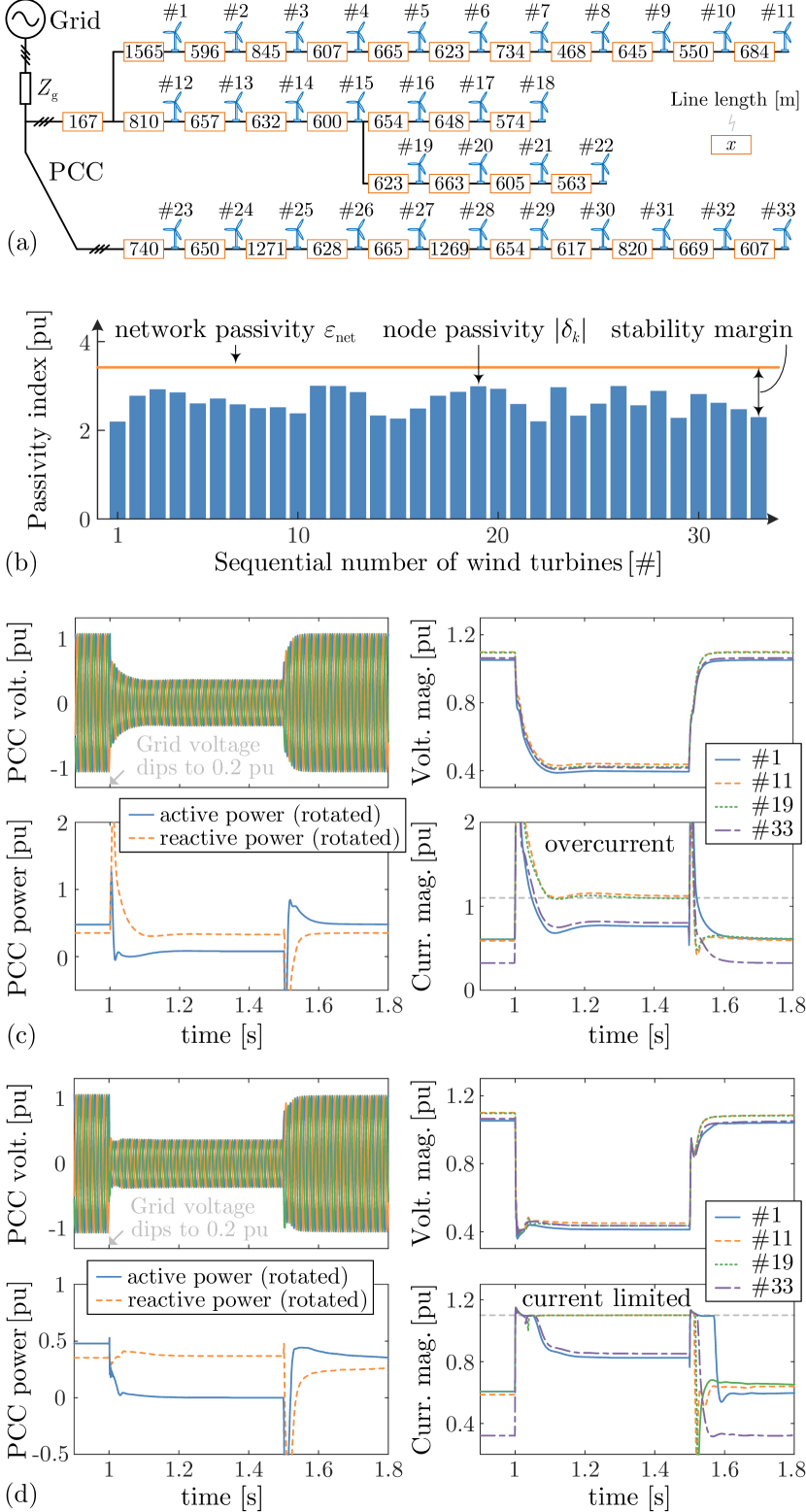
We illustrate the calculation of passivity indices and their application in ensuring the transient stability of a wind power plant (WPP). Our case study is based on a real WPP layout depicted in Fig. 2(a) [2], where all wind turbine converters are dVOC-controlled. Power setpoints are randomly selected between $[0,\sqrt{2}]$ pu but scaled down to $1.0$ pu if the apparent power exceeds this threshold. Voltage setpoints are uniformly set to $1.0$ pu. Moreover, we employ $\eta_{k}=0.04\times 100\pi$ rad/s and $\alpha_{k}=2$ pu. The grid impedance is $0.05+j0.15$ pu, and the collector line parameters are $0.1153\,\Omega$/${\rm km}$,$1.05\times 10^{-3}\,{\rm H}$/${\rm km}$.

The node passivity indices are conservatively estimated by the first two terms of (5), where $\delta_{k}<0$ happens typically, implying a shortage of node passivity. The network passivity index is computed by (8), $\varepsilon_{\rm net}>0$, contributed by the grid impedance, the collector line impedance, the step-up transformer impedance, and the virtual impedance emulated in converters. Since the equivalent grid impedance usually changes when a grid fault occurs, the changed impedance should be used when evaluating the network passivity. Moreover, the virtual impedance appearing for fault current limiting should also be incorporated into the network representation.

Fig. 2(b) displays the calculated passivity indices, where the value of $(\varepsilon_{\rm net}-\absolutevalue{\delta_{k}})$ represents the stability margin of each generating unit, $\varepsilon_{\rm net}-\absolutevalue{\delta_{k}}>0$ for all units satisfying the decentralized stability conditions. The simulation results in Fig. 2(c) and (d) based on MATLAB/Simulink validate the transient stability of the system under a grid voltage dip, where the complete control dynamics are included, and the converters are average-valued, with fixed DC voltages and sufficiently fast inner-loop dynamics. To address the overcurrent in Fig. 2(c) while maintaining the grid-forming operation of the converters, we apply a saturation-informed current limiting strategy [13] in Fig. 2(d). Alternatively, one can use the classical virtual-impedance current limiting strategy [8]. Both strategies result in an equivalent circuit with a virtual impedance and an internal voltage source. Our decentralized stability conditions readily apply to the equivalent circuit network with the virtual impedance. We have also validated the stability of the system across different voltage dip depths.

V Conclusion

We have analytically studied the transient stability of multi-converter grid-connected systems employing the grid-forming dVOC control. The passivity of dVOC in large-signal form makes itself noteworthy in stability guarantees. By leveraging the passivity index of the dVOC-controlled node dynamics and the inherent passivity of the network, we develop decentralized stability conditions, serving as a fast and effective tool for controller parameter tuning, transient stability guarantees, and stability margin assessment.

References

  • [1] T. Liu, Y. Song, L. Zhu, and D. J. Hill, “Stability and control of power grids,” Annu. Rev. Control Robot. Auton. Syst., vol. 5, no. 1, pp. 689–716, 2022.
  • [2] W. Li, P. Chao, X. Liang, J. Ma, D. Xu, and X. Jin, “A practical equivalent method for DFIG wind farms,” IEEE Trans. Sustain. Energy, vol. 9, no. 2, pp. 610–620, 2017.
  • [3] C. Spanias and I. Lestas, “A system reference frame approach for stability analysis and control of power grids,” IEEE Trans. Power Syst., vol. 34, no. 2, pp. 1105–1115, 2019.
  • [4] K. Dey and A. M. Kulkarni, “Passivity-based decentralized criteria for small-signal stability of power systems with converter-interfaced generation,” IEEE Trans. Power Syst., vol. 38, no. 3, pp. 2820–2833, 2023.
  • [5] P. Yang, F. Liu, Z. Wang, and C. Shen, “Distributed stability conditions for power systems with heterogeneous nonlinear bus dynamics,” IEEE Trans. Power Syst., vol. 35, no. 3, pp. 2313–2324, 2020.
  • [6] H. K. Khalil, Nonlinear Systems, 3rd ed.   Englewood Cliffs, NJ, USA: Prentice-Hall, 2002.
  • [7] X. He, L. Huang, I. Subotić, V. Häberle, and F. Dörfler, “Quantitative stability conditions for grid-forming converters with complex droop control,” 2023, submitted to IEEE Trans. Power Electron. [Online]. Available: https://arxiv.org/pdf/2310.09933.pdf
  • [8] T. Qoria, F. Gruson, F. Colas, X. Kestelyn, and X. Guillaud, “Current limiting algorithms and transient stability analysis of grid-forming VSCs,” Electr. Power Syst. Res., vol. 189, p. 106726, 2020.
  • [9] K. De Brabandere, B. Bolsens, J. Van den Keybus, A. Woyte, J. Driesen, and R. Belmans, “A voltage and frequency droop control method for parallel inverters,” IEEE Trans. Power Electron., vol. 22, no. 4, pp. 1107–1115, 2007.
  • [10] L. Kong, Y. Xue, L. Qiao, and F. Wang, “Control design of passive grid-forming inverters in port-hamiltonian framework,” IEEE Trans. Power Electron., pp. 1–15, 2023.
  • [11] W. Dong, H. Xin, D. Wu, and L. Huang, “Small signal stability analysis of multi-infeed power electronic systems based on grid strength assessment,” IEEE Trans. Power Syst., vol. 34, no. 2, pp. 1393–1403, 2019.
  • [12] M. Colombino, D. Groß, J.-S. Brouillon, and F. Dörfler, “Global phase and magnitude synchronization of coupled oscillators with application to the control of grid-forming power inverters,” IEEE Trans. Autom. Control, vol. 64, no. 11, pp. 4496–4511, 2019.
  • [13] M. A. Desai, X. He, L. Huang, and F. Dörfler, “Saturation-informed current-limiting control for grid-forming converters,” 2023, submitted to Electr. Power Syst. Res. and patent pending.