Quantitative Stability Conditions for Grid-Forming Converters With Complex Droop Control

Abstract

In this paper, we study analytically the transient stability of grid-connected distributed generation systems with grid-forming (GFM) complex droop control, also known as dispatchable virtual oscillator control (dVOC). We prove theoretically that complex droop control, as a state-of-the-art GFM control, always possesses steady-state equilibria whereas classical droop control does not. We provide quantitative conditions for complex droop control maintaining transient stability (global asymptotic stability) under grid disturbances, which is beyond the well-established local (non-global) stability for classical droop control. For the transient instability of complex droop control, we reveal that the unstable trajectories are bounded, manifesting as limit cycle oscillations. Moreover, we extend our stability results from second-order GFM control dynamics to full-order system dynamics that additionally encompass both circuit electromagnetic transients and inner-loop dynamics. Our theoretical results contribute an insightful understanding of the transient stability and instability of complex droop control and offer practical guidelines for parameter tuning and stability guarantees.

I Introduction

THE ubiquitous penetration of distributed generation in power grids has been displacing a substantial number of centralized synchronous generators. Grid-forming (GFM) responsibilities initially shouldered by synchronous generators for establishing and regulating grid frequency and voltage are increasingly being transferred to distributed generation systems. Therefore, grid-forming converters, serving as a powerful grid connection interface for distributed generation, are becoming indispensable assets in modern power systems [1]. Under large disturbances, GFM converters need to maintain transient stability and provide continuous support for power grid operation [2]. Since transient stability involves a wide range of changes in the system operating state, the nonlinear dynamic characteristics of GFM converters play a significant role. Moreover, in comparison to small-signal local stability, transient stability faces greater challenges in nonlinear analysis, simulation, and control [3].

Concerning early-stage GFM control strategies, e.g., classical p/f and q/v droop control [4, 5, 6, 7, 8, 9] and virtual synchronous machine (VSM) [10, 11, 12, 13], their stability in islanded or grid-connected scenarios has been studied extensively in the literature, as summarized in Table I(a). In particular, since the development of classical droop control is based on the single-input single-output (SISO) decoupling and linear approximation of the network power flow, it is generally observed that classical droop control schemes exhibit good small-signal/local stability performance [14]. In other words, their local stability can be guaranteed theoretically [4, 5, 6]. However, the large-signal/transient response behavior of classical droop control is usually inferior, with rigorous guarantees of large-signal/transient/global stability established only under assumptions of inductive networks and/or fixed voltage magnitudes [7, 11]. The VSM strategy, which follows the same droop philosophy in its building block, further introduces virtual inertia to improve the frequency response performance. The resulting second-order control structure, however, may deteriorate transient stability [15], where the region of attraction (ROA) and the critical fault clearing time (CCT) are typically the main concerns [10].

TABLE I: Past Studies on Stability of Typical GFM Controls

Ref.	Year	Type	Assumption	Method	Result	Publ.1
(a) Elementary GFM controls
[4]	2012	1st-order Kuramoto model	Volt. fixed, network inductive	Linearization	Local	Ctrl.
[5]	2012	2nd-order Kuramoto model	Volt. fixed	Singular perturbation, contraction	Local	Ctrl.
[6]	2013	p/f droop in structure- preserving network	Volt. fixed, network inductive	Graph- theoretic methods, linearization	Local	PS
[7]	2014	p/f and q/v droop	Network inductive	Lyapunov- like analysis	Local and global	Ctrl.
[8]	2019	p/f droop	Volt. fixed, network inductive	Phase portrait	Global	PE
[9]	2019	Current- limited p/f droop	Volt. fixed, network inductive	Power-angle curve analysis	ROA	PS
[10]	2019	VSM	Static q/v relationship	Energy function	ROA	PS
[11]	2019	VSM	Volt. fixed, network inductive	Multivariable cell structure, Leonov func.	Almost global	Ctrl.
[12]	2020	VSM	Volt. fixed, network inductive	Energy function	ROA	PS
[13]	2022	Current- limited VSM	Volt. fixed, network inductive	Power-angle curve analysis	ROA	PS
(b) Advanced GFM controls
[16] [17] [18] [19]	2019 2019 2021 2022	dVOC	Consistent setpoints	Lyapunov- like analysis	Almost global	Ctrl.
[20]	2021	dVOC	Network inductive	Phase portrait	Global	PE
[21]	2021	dVOC	Network static	3D phase portrait	Global	PE
[22]	2018	Matching control	Grid signal available	Hamiltonian analysis	Global	PE
[23]	2022	Hybrid angle control	Voltage fixed	Lyapunov analysis	Almost global	Ctrl.
[24]	2022	Power-bal. dual-port GFM control	Volt. fixed, network inductive	LaSalle invariance principle	Local	Ctrl.

• Publication communities include control community (Ctrl.), power electronics community (PE), and power systems community (PS).

In recent years, advanced GFM controls have been widely explored, e.g., dispatchable virtual oscillator control (dVOC) [16, 17, 18, 19, 20, 21], matching control [22], hybrid angle control [23], and dual-port GFM control [24], as shown in Table I(b). These controls are well-designed to address various control objectives and ensure stability, particularly global stability. Among these controls, dVOC, developed in [16], has attracted increasing attention due to its unique capabilities in synchronization and voltage stabilization. Our recent work [25] has reformulated dVOC equivalently as complex-power complex-frequency droop control (complex droop control for short), based on a novel concept termed “complex frequency” [26]. Complex frequency is a unifying/compact representation of angular frequency and the rate of change of voltage. In this sense, complex droop control associates active and reactive power inputs to frequency and rate-of-change-of-voltage outputs with a non-trivial coupling. As a consequence, the control is structurally multivariable and also intrinsically nonlinear, in contrast to SISO linear loops in classical droop control or VSM. In particular, complex droop control can effectively handle the inherent coupling and nonlinearity in the network’s active and reactive power flows. In [16, 17, 18, 19], a more general global stability guarantee has been established for dVOC, which goes beyond the local stability of classical droop control and beyond the scenarios of inductive networks and/or fixed voltages. The stability results have been experimentally validated and often reproduced [27, 28].

While the stability of dVOC (i.e., complex droop control) in converter-based islanded systems has been well studied in [16, 17, 18, 19], the stability in grid connection remains unaddressed theoretically. In this regard, the grid voltage appears as a forced input to the nonlinear GFM control dynamics, altering both the dynamic response and the steady-state solution, presenting different challenges in nonlinear stability analysis. As can be seen in Table I(b), the phase portrait approach has been applied in [20, 21] to geometrically observe the transient behavior of dVOC under grid disturbances. However, this approach relies on numerical solutions of dynamic trajectories, and it lacks the capability to yield analytical stability conditions. To the best of our knowledge, the analytical results of transient stability for dVOC in a grid-connected context remain absent in the literature. The absence of theoretical results hinders the application of dVOC in the control of grid-connected renewable/distributed energy resources, high-voltage DC systems, smart loads, etc. Likewise, there is limited attention on the transient instability behavior analysis for dVOC. Another big research gap exists when it comes to the analytical exploration of transient stability of full-order dynamics in GFM converters in grid connection. Namely, many prior studies as in Table I have focused solely on the dynamics of GFM controls while overlooking both circuit electromagnetic transients and inner-loop dynamics. Existing small-signal stability conditions considering full-order converter dynamics, e.g., [29, 30, 31], which are dependent on equilibrium points and limited to the small-signal regime, cannot guarantee transient stability. Quantitative conditions for transient stability remain absent in the literature.

In this paper, our objectives are threefold: firstly, to explore the transient stability condition of complex droop control (i.e., dVOC) in a reduced-order grid-connected converter system; secondly, to investigate how the transient instability of complex droop control behaves; and thirdly, to examine the transient stability condition for full-order system dynamics. The contributions of this study are summarized as follows:

• We prove that complex droop control always possesses steady-state equilibrium points whereas classical droop control and VSM do not. Additionally, complex droop control maintains transient stability under our provided quantitative parametric stability conditions.

• We prove that the trajectories of complex droop control are bounded and the transient instability of complex droop control manifests as limit cycle oscillations.

• We prove that the full-order system dynamics, which encompasses GFM control dynamics, circuit electromagnetic dynamics, and inner-loop dynamics, maintain transient stability within a wide region of attraction, and we provide quantitative parametric conditions for the transient stability of the full-order system dynamics.

The remainder of this paper proceeds as follows. The description of complex droop control and the comparison with classical droop control are presented in Section II. Full-order and reduced-order system models are formulated in Section III, where the stability problem statement is also included. Section IV presents the transient stability and instability analysis for the reduced-order system, and Section V extends the stability results to the full-order system. Case studies are presented in Section VI, and Section VII concludes this paper.

II Preliminaries

II-A Definitions of Relevant Complex Variables

1) Voltage Vector and Complex Voltage: Under three-phase balanced conditions, the voltage at the converter terminal node can be expressed in $\alpha\beta$ rectangular coordinates as

$$\boldsymbol{v}\coloneqq[v_{\alpha}\ \ v_{\beta}]^{\mathsf{T}}\coloneqq[v\cos\theta\ \ v\sin\theta]^{\mathsf{T}},$$ (1)

where $v$ denotes the voltage amplitude and $\theta$ denotes the rotational phase-angle. We define the complex voltage vector $\underline{v}$ in the associated complex vector coordinate as

$$\underline{v}\coloneqq v_{\alpha}+jv_{\beta}=v\left(\cos\theta+j\sin\theta\right)={v}{e^{j{\theta}}},$$ (2)

where the underline indicates complex-valued variables.

2) Complex Angle: Consider the complex voltage vector in (2) with $v>0$. We define the complex angle vector $\underline{\vartheta}$ [26] as

$$\underline{\vartheta}\coloneqq{u}+j{\theta}\coloneqq\ln{v}+j{\theta},\quad\Rightarrow\quad\underline{v}=e^{\underline{\vartheta}},$$ (3)

where $u\coloneqq\ln{v}$ is defined as voltage logarithm. The complex-angle $\underline{\vartheta}$ contains two-dimensional information on the amplitude and angle of the voltage. From the definition of the complex angle in (3), it follows that $\underline{v}=e^{\underline{\vartheta}}$, which serves as a transformation between complex-voltage coordinates and complex-angle coordinates.

3) Complex Frequency: Based on the time derivative of ${\underline{\vartheta}}$, we define the complex frequency $\underline{\varpi}$ [26] as

$$\underline{\varpi}\coloneqq\dot{\underline{\vartheta}}={\dot{v}}/v+j{\dot{\theta}}={\dot{\underline{v}}}/\underline{v}=:{\varepsilon}+j{\omega},$$ (4)

where $\varepsilon=\dot{v}/{v}$ is the rate of change of voltage, and $\omega$ denotes the angular frequency. More precisely, $\varepsilon$ denotes the radial frequency that represents the change in the amplitude while $\omega$ represents the standard angular frequency. This outlines a geometrical interpretation of the complex frequency.

4) Normalized Complex Power: In conventional power systems, the balance of active power indicates frequency synchronization. To indicate “complex-frequency” synchronization, we define a “complex version” of power. As in [25], the complex, conjugated, and normalized power $\overline{\underline{\varsigma}}$ is defined as

$$\overline{\underline{\varsigma}}\coloneqq\overline{\underline{s}}/v^{2}=(p-jq)/v^{2}={\overline{\underline{v}}}\,{\underline{i}}/v^{2}={\underline{i}}/{\underline{v}},$$ (5)

where the overline indicates conjugate variables, $\underline{s}$ is standard complex power with $p$ and $q$ being active and reactive power, and $\underline{i}$ represents output current. For brevity of notation, we further define normalized active and reactive power as $\rho\coloneqq p/v^{2}=\Re{\overline{\underline{\varsigma}}},\,\sigma\coloneqq q/v^{2}=-\Im{\overline{\underline{\varsigma}}}$, which will be employed in complex droop control in the following.

II-B From Classical Droop Control to Complex Droop Control

1) Classical Droop Control: We review classical droop control, which is seen as an elementary GFM control,

$$\dot{v} =\eta\left(q_{\varphi}^{\star}-q_{\varphi}\right)+\eta\alpha\left(v^{\star}-v\right),$$ (6a)

$$\dot{{\theta}} ={\omega}_{0}+\eta\left(p_{\varphi}^{\star}-p_{\varphi}\right),$$ (6b)

where $\eta\in\mathbb{R}_{>0}$ is the power droop gain, $\alpha\in\mathbb{R}_{\geq 0}$ is the voltage droop gain, $\omega_{0}$ is the nominal frequency, and the variables with superscript ^⋆ denote the associated setpoints. It is important to note that the power setpoints and feedback can be rotated by a tunable angle $\varphi$ to adapt to the network impedance characteristics [32]. Namely,

$$p_{\varphi}^{\star}+jq_{\varphi}^{\star} \coloneqq e^{j(\pi/2-\varphi)}(p^{\star}+jq^{\star}),$$ (7a)

$$p_{\varphi}+jq_{\varphi} \coloneqq e^{j(\pi/2-\varphi)}(p+jq),$$ (7b)

where the rotation angle ${\varphi}$ is chosen typically as the network impedance angle ${\varphi}=\arctan(\omega_{0}\ell/r)\in[0,\pi/2]$. For the dominantly inductive network case, ${\varphi}=\pi/2$ results in the standard decoupled p/f and q/v droop control.

2) Complex Droop Control: We augment the p/f droop control in (6b) into a complex-power complex-frequency multivariable droop control (complex droop control for short) as

$$\dot{\underline{\vartheta}}=\underline{\varpi}_{0}+\eta e^{j\varphi}\left(\overline{\underline{\varsigma}}^{\star}-\overline{\underline{\varsigma}}\right),$$ (8)

where $\underline{\varpi}_{0}\coloneqq j{\omega}_{0}$ denotes the nominal complex frequency, $\eta\in\mathbb{R}_{>0}$, $e^{j\varphi}$ denotes the rotation operator to adapt to the network impedance characteristics, and moreover, the complex power setpoint is given by $\overline{\underline{\varsigma}}^{\star}\coloneqq\rho^{\star}-j\sigma^{\star}\coloneqq(p^{\star}-jq^{\star})/v^{\star 2}$. The second term in (8) denotes the droop gain multiplied by the imbalance of complex power, which is to regulate the complex-frequency dynamics. From angular frequency to complex frequency, this complex droop control can be seen as an advancement of the elementary p/f droop control.

The complex droop control in (8) is only able to regulate the rate of change of voltage as well as the angular frequency. To directly regulate the voltage amplitude, we introduce an amplitude regulation-enabled complex droop control [19] as

$$\dot{\underline{\vartheta}}=\underline{\varpi}_{0}+\eta e^{j\varphi}\left(\overline{\underline{\varsigma}}^{\star}-\overline{\underline{\varsigma}}\right)+\eta\alpha\tfrac{v^{\star 2}-v^{2}}{v^{\star 2}},$$ (9)

where $\alpha\in\mathbb{R}_{\geq 0}$ is the voltage regulation gain, $v^{\star}$ denotes the voltage setpoint, $v=e^{\Re{\underline{\vartheta}}}$ denotes the voltage amplitude, and $(v^{\star 2}-v^{2})$ represents the voltage regulation deviation (another alternative is $(v^{\star}-v)$ [16]). We rewrite (9) in real-valued polar coordinates as

$${\dot{v}}/{v} =\eta\left(\sigma_{\varphi}^{\star}-\sigma_{\varphi}\right)+\eta\alpha\left({v^{\star 2}-v^{2}}\right)/{v^{\star 2}},$$ (10a)

$$\dot{\theta} =\omega_{0}+\eta\left(\rho_{\varphi}^{\star}-\rho_{\varphi}\right),$$ (10b)

where the subscript $\varphi$ indicates the rotated power, i.e.,

$$\sigma_{\varphi}^{\star}+j\rho_{\varphi}^{\star} \coloneqq e^{j\varphi}\overline{\underline{\varsigma}}^{\star} =(q_{\varphi}^{\star}+jp_{\varphi}^{\star})/{v^{\star 2}},$$ (11a)

$$\sigma_{\varphi}+j\rho_{\varphi} \coloneqq e^{j\varphi}\overline{\underline{\varsigma}} =(q_{\varphi}+jp_{\varphi})/{v^{2}}.$$ (11b)

The second equalities in (11a) and (11b) follow from the preceding related definitions.

The complex droop control in (9) provides two control modes [33], i.e., either with or without the voltage regulation term. The voltage-following mode is given by $\alpha=0$. The operation of this mode must rely on other voltage sources since the voltage amplitude is not controlled (though the frequency is controlled in a droop fashion). The voltage-forming mode, also termed grid-forming mode [33], is given by $\alpha\neq 0$, where both the frequency and the voltage amplitude are controlled in a droop fashion.

Remark 1 (Differences between classical and complex droop controls).

The complex droop control in (10) differs from the classical droop control in (6), where two relevant differences are identified as follows.

• The derivative of $v$ differs from that of $\ln v$, i.e., $\dot{v}/v$.

• The standard power feedback is different from the normalized power feedback.

The differences have a minor impact on the steady-state droop performance in the vicinity of $v\approx v^{\star}\approx 1.0$ pu, but they exert a substantial and positive impact on the transient stability due to the nonlinear coupling from $p_{\varphi}$ and $q_{\varphi}$ to $v$ and $\theta$ in the large-signal regime. These differences allow us to establish global asymptotic stability for complex droop control in this study, a result that remains unestablished in the general case for classical droop control [7, 11].

Remark 2 (Equivalence to dVOC [25]).

We recall the mathematical equivalence between complex droop control and dVOC [25], as illustrated in Fig. 1. Considering ${\underline{\dot{v}}}/{\underline{v}}=\underline{\dot{\vartheta}}$ following from the coordinate transformation $\underline{v}=e^{\underline{\vartheta}}$, we can rewrite the complex droop control in (9), from complex-angle coordinates to complex-voltage coordinates, as follows

$$\dot{\underline{v}}=\underline{\varpi}_{0}\underline{v}+\eta e^{j\varphi}\left(\overline{\underline{\varsigma}}^{\star}\underline{v}-\underline{i}\right)+\eta\alpha\tfrac{v^{\star 2}-v^{2}}{v^{\star 2}}\underline{v},$$ (12)

where $\underline{i}=\overline{\underline{\varsigma}}\,\underline{v}$ follows from (5). The controller in (12) is the complex variable version of the dVOC developed in [17]. In consideration of equivalence, the terms “dVOC” and “complex droop control” can be used equivalently.

III Modeling and Stability Problem Statement

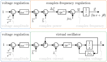
Figure 1: Complex droop control in complex-angle coordinates and equivalent dVOC in complex-voltage coordinates.

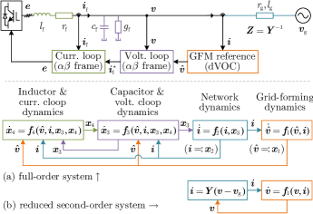
Figure 2: A grid-connected converter system with dVOC (i.e., complex droop control) and inner control loops. (a) The full-order model in (18) in a multi-time-scale nested form. (b) The reduced second-order model in (19) with GFM dynamics solely (further detailed in Fig. 3).

Consider a grid-connected converter with complex droop control, as shown in Fig. 2. We first derive its full-order model, which includes the GFM control dynamics, the network electromagnetic dynamics, the filter dynamics, the voltage loop dynamics, and the current loop dynamics. For ease of modeling and analysis, we adopt the grid synchronous reference frame oriented by the grid voltage vector angle $\theta_{\rm g}$, and we consider that all AC signals are already transformed to the grid synchronous reference frame. We define the main variables and parameters utilized throughout this paper in Table II. In the following, we use vectors $[a\enspace b]^{\mathsf{T}}$ or matrices $[\begin{smallmatrix}a&-b\\ b&a\end{smallmatrix}]$ to equivalently represent to $a+jb$ for ease of understanding.

TABLE II: Definitions of Symbols, Variables, and Parameters

Symbol	Description	Symbol	Description
$v$	Voltage amplitude	$\eta>0$	Power droop gain
$\theta$	Voltage angle	$\alpha\geq 0$	Voltage droop gain
$\underline{v}\coloneqq ve^{j\theta}$	Complex voltage	$r_{\rm g}$	Grid resistance
$\underline{\vartheta}\coloneqq\ln v+j\theta$	Complex angle	$l_{\rm g}$	Grid inductance
$\underline{\varpi}\coloneqq\dot{\underline{\vartheta}}$	Complex frequency	$\underline{z}$	$r_{\rm g}+j\omega_{\rm g}l_{\rm g}$
$\varepsilon\coloneqq\dot{v}/v$	Rate of change of voltage	$\underline{y}$	$\underline{z}^{-1}$
$\omega\coloneqq\dot{\theta}$	Angular frequency	$\boldsymbol{Z}$	$[\begin{smallmatrix}r_{\rm g}&-\omega_{\rm g}l_{\rm g}\\ \omega_{\rm g}l_{\rm g}&r_{\rm g}\end{smallmatrix}]$
$\underline{i}$	Complex current	$\boldsymbol{Y}$	$\boldsymbol{Z}^{-1}$
$\underline{s}\coloneqq p+jq$	Complex power	$r_{\rm f}$	Filter resistance
$\underline{\varsigma}\coloneqq\underline{s}/v^{2}$	Normalized power	$l_{\rm f}$	Filter inductance
$\rho\coloneqq p/v^{2}$	Normalized $p$	$g_{\rm f}$	Filter conductance
$\sigma\coloneqq q/v^{2}$	Normalized $q$	$c_{\rm f}$	Filter capacitance
$\varphi$	Rotation angle	$\boldsymbol{Y}_{\rm f}$	$[\begin{smallmatrix}g_{\rm f}&-\omega_{\rm g}c_{\rm f}\\ \omega_{\rm g}c_{\rm f}&g_{\rm f}\end{smallmatrix}]$
$p_{\varphi}+jq_{\varphi}$	Rotated by $\varphi$	$\boldsymbol{Z}_{\rm f}$	$[\begin{smallmatrix}r_{\rm f}&-\omega_{\rm g}l_{\rm f}\\ \omega_{\rm g}l_{\rm f}&r_{\rm f}\end{smallmatrix}]$
$\rho_{\varphi}+j\sigma_{\varphi}$	Rotated by $\varphi$	$\boldsymbol{i}_{\rm f}$	Inductor current
$\boldsymbol{v}_{\rm g}\coloneqq[v_{\rm g}\enspace 0]^{\mathsf{T}}$	Grid voltage	$\boldsymbol{i}_{\rm f}^{\star}$	Reference for $\boldsymbol{i}_{\rm f}$
$\hat{\boldsymbol{v}}\coloneqq[\hat{v}_{\rm d}\enspace\hat{v}_{\rm q}]^{\mathsf{T}}$	Reference voltage	$\boldsymbol{e}$	Internal voltage
$\boldsymbol{v}\coloneqq[v_{\rm d}\enspace v_{\rm q}]^{\mathsf{T}}$	Capacitor voltage	$\boldsymbol{I}_{2}$	$[\begin{smallmatrix}1&0\\ 0&1\end{smallmatrix}]$
$\boldsymbol{v}_{\rm s}$	Steady-state voltage	$\boldsymbol{J}$	$[\begin{smallmatrix}0&-1\\ 1&0\end{smallmatrix}]$
$\boldsymbol{i}$	Output current	$\boldsymbol{R}_{\varphi}$	$[\begin{smallmatrix}\cos\varphi&-\sin\varphi\\ \sin\varphi&\cos\varphi\end{smallmatrix}]$
$\Re{}$	Real part	$\boldsymbol{S}_{\varphi}^{\star}$	$[\begin{smallmatrix}\sigma_{\varphi}^{\star}&-\rho_{\varphi}^{\star}\\ \rho_{\varphi}^{\star}&\sigma_{\varphi}^{\star}\end{smallmatrix}]$
$\Im{}$	Imaginary part	$\boldsymbol{\Phi}(\hat{\boldsymbol{v}})$	$\frac{v^{\star 2}-\norm{\hat{\boldsymbol{v}}}^{2}}{v^{\star 2}}\boldsymbol{I}_{2}$
$()^{\mathsf{T}}$	Transpose	$\omega_{\rm g},\theta_{\rm g}$	Grid freq., angle
$()^{\mathsf{H}}$	Hermitian transpose	$\omega_{\Delta}$	$\omega_{0}-\omega_{\rm g}$
$()^{\star}$	Setpoint	$\boldsymbol{Y}_{\varphi}$	$\boldsymbol{R}_{\varphi}\boldsymbol{Y}$
$()_{\rm s}$	Steady state	$[\begin{smallmatrix}\kappa_{\rm r}&-\kappa_{\rm i}\\ \kappa_{\rm i}&\kappa_{\rm r}\end{smallmatrix}]$	$\boldsymbol{S}_{\varphi}^{\star}-\boldsymbol{Y}_{\varphi}$

III-A Full-Order System With Multi-Time-Scale Dynamics

GFM Reference Model: The complex droop control in (12) serves as a GFM reference model to generate the reference voltage $\hat{\boldsymbol{v}}$ for the inner voltage loop, in vector form, as

$$\dot{\hat{\boldsymbol{v}}}=\omega_{\Delta}\boldsymbol{J}\hat{\boldsymbol{v}}+\eta\boldsymbol{S}_{\varphi}^{\star}\hat{\boldsymbol{v}}-\eta\boldsymbol{R}_{\varphi}\boldsymbol{i}+\eta\alpha\boldsymbol{\Phi}(\hat{\boldsymbol{v}})\hat{\boldsymbol{v}},$$ (13)

where $\boldsymbol{S}_{\varphi}^{\star}$, as a matrix, encodes the rotated power setpoint $e^{j\varphi}\overline{\underline{\varsigma}}^{\star}$, $\boldsymbol{R}_{\varphi}$ encodes $e^{j\varphi}$, $\boldsymbol{\Phi}(\hat{\boldsymbol{v}})\coloneqq\frac{v^{\star 2}-\norm{\hat{\boldsymbol{v}}}^{2}}{v^{\star 2}}\boldsymbol{I}_{2}$, and $\norm{\cdot}$ denotes Euclidean distance. We refer to Table II for a complete description of variables/parameters.

Network Dynamics: The network electromagnetic dynamics are given as

$$l_{\rm g}\dot{\boldsymbol{i}}+\boldsymbol{Z}\boldsymbol{i}=\boldsymbol{v}-\boldsymbol{v}_{\rm g},$$ (14)

with the grid voltage $\boldsymbol{v}_{\rm g}\coloneqq[v_{\rm g}\enspace 0]^{\mathsf{T}}$.

Filter Capacitor and Inductor Dynamics: The filter capacitor and inductor dynamics are given as

$$c_{\rm f}\dot{\boldsymbol{v}}+\boldsymbol{Y}_{\rm f}\boldsymbol{v}+\boldsymbol{i} =\boldsymbol{i}_{\rm f},$$ (15a)

$$l_{\rm f}\dot{\boldsymbol{i}}_{\rm f}+\boldsymbol{Z}_{\rm f}\boldsymbol{i}_{\rm f}+\boldsymbol{v} =\boldsymbol{e},$$ (15b)

with the converter-side current $\boldsymbol{i}_{\rm f}$ and the internal voltage $\boldsymbol{e}$.

Voltage Controller: Consider a voltage reference tracking controller with feedforward compensation, which can be directly implemented in $\alpha\beta$ coordinates. When transformed into the grid reference frame, it is given as [18]

$$\dot{\boldsymbol{\zeta}}_{\rm v} =\omega_{\Delta}\boldsymbol{J}\boldsymbol{\zeta}_{\rm v}+\boldsymbol{v}-\hat{\boldsymbol{v}},$$ (16a)

$$\boldsymbol{i}_{\rm f}^{\star} =-k_{\rm p}^{\rm v}(\boldsymbol{v}-\hat{\boldsymbol{v}})-k_{\rm r}^{\rm v}\boldsymbol{\zeta}_{\rm v}+\boldsymbol{Y}_{\rm f}\boldsymbol{v}+\boldsymbol{i},$$ (16b)

where ${\boldsymbol{\zeta}}_{\rm v}$ stands for the resonant integrator state, $(\boldsymbol{Y}_{\rm f}\boldsymbol{v}+\boldsymbol{i})$ denotes the feedforward compensation, and $k_{\rm p}^{\rm v}\in\mathbb{R}_{>0}$ and $k_{\rm r}^{\rm v}\in\mathbb{R}_{>0}$ are the voltage control gains.

Current Controller: Similarly, the current reference tracking controller in the grid reference frame is given as

$$\dot{\boldsymbol{\zeta}}_{\rm c} =\omega_{\Delta}\boldsymbol{J}\boldsymbol{\zeta}_{\rm c}+\boldsymbol{i}_{\rm f}-\boldsymbol{i}_{\rm f}^{\star},$$ (17a)

$$\boldsymbol{e} =-k_{\rm p}^{\rm c}(\boldsymbol{i}_{\rm f}-\boldsymbol{i}_{\rm f}^{\star})-k_{\rm r}^{\rm c}\boldsymbol{\zeta}_{\rm c}+\boldsymbol{Z}_{\rm f}\boldsymbol{i}_{\rm f}+\boldsymbol{v},$$ (17b)

where ${\boldsymbol{\zeta}}_{\rm c}$ stands for the resonant integrator state, $(\boldsymbol{Z}_{\rm f}\boldsymbol{i}_{\rm f}+\boldsymbol{v})$ is the feedforward compensation, and $k_{\rm p}^{\rm c}\in\mathbb{R}_{>0}$ and $k_{\rm r}^{\rm c}\in\mathbb{R}_{>0}$ are the current control gains.

From (13) to (17), the full-order (twelfth-order) system is formulated as

$$\tfrac{\rm d}{{\rm d}t}\underbrace{\hat{\boldsymbol{v}}}_{=:\boldsymbol{x}_{1}} =\underbrace{\omega_{\Delta}\boldsymbol{J}\hat{\boldsymbol{v}}+\eta\boldsymbol{S}_{\varphi}^{\star}\hat{\boldsymbol{v}}-\eta\boldsymbol{R}_{\varphi}\boldsymbol{i}+\eta\alpha\boldsymbol{\Phi}(\hat{\boldsymbol{v}})\hat{\boldsymbol{v}}}_{=:\,\boldsymbol{f}_{1}(\boldsymbol{x}_{1},\boldsymbol{x}_{2})},$$ (18a)

$$\tfrac{\rm d}{{\rm d}t}\underbrace{\boldsymbol{i}}_{=:\boldsymbol{x}_{2}} =\underbrace{l_{\rm g}^{-1}(-\boldsymbol{Z}\boldsymbol{i}+\boldsymbol{v}-\boldsymbol{v}_{\rm g})}_{=:\,\boldsymbol{f}_{2}(\boldsymbol{x}_{1},\boldsymbol{x}_{2},\boldsymbol{x}_{3})},$$ (18b)

$$\tfrac{\rm d}{{\rm d}t}\underbrace{\begin{bmatrix}{\boldsymbol{v}}\\ {\boldsymbol{\zeta}}_{\rm v}\end{bmatrix}}_{=:\boldsymbol{x}_{3}} =\underbrace{\begin{bmatrix}c_{\rm f}^{-1}(-\boldsymbol{Y}_{\rm f}\boldsymbol{v}-\boldsymbol{i}+\boldsymbol{i}_{\rm f})\\ \omega_{\Delta}\boldsymbol{J}\boldsymbol{\zeta}_{\rm v}+\boldsymbol{v}-\hat{\boldsymbol{v}}\end{bmatrix}}_{=:\,\boldsymbol{f}_{3}(\boldsymbol{x}_{1},\boldsymbol{x}_{2},\boldsymbol{x}_{3},\boldsymbol{x}_{4})},$$ (18c)

$$\tfrac{\rm d}{{\rm d}t}\underbrace{\begin{bmatrix}{\boldsymbol{i}}_{\rm f}\\ {\boldsymbol{\zeta}}_{\rm c}\end{bmatrix}}_{=:\boldsymbol{x}_{4}} =\underbrace{\begin{bmatrix}l_{\rm f}^{-1}(-k_{\rm p}^{\rm c}(\boldsymbol{i}_{\rm f}-\boldsymbol{i}_{\rm f}^{\star})-k_{\rm r}^{\rm c}\boldsymbol{\zeta}_{\rm c})\\ \omega_{\Delta}\boldsymbol{J}\boldsymbol{\zeta}_{\rm c}+\boldsymbol{i}_{\rm f}-\boldsymbol{i}_{\rm f}^{\star}\end{bmatrix}}_{=:\,\boldsymbol{f}_{4}(\boldsymbol{x}_{1},\boldsymbol{x}_{2},\boldsymbol{x}_{3},\boldsymbol{x}_{4})},$$ (18d)

$$\boldsymbol{i}_{\rm f}^{\star} =-k_{\rm p}^{\rm v}(\boldsymbol{v}-\hat{\boldsymbol{v}})-k_{\rm r}^{\rm v}\boldsymbol{\zeta}_{\rm v}+\boldsymbol{Y}_{\rm f}\boldsymbol{v}+\boldsymbol{i},$$ (18e)

which is also graphically illustrated in Fig. 2 from the slowest to the fastest dynamics in the form of a nested block diagram. We note that $\boldsymbol{v}_{\rm g}$ plays as a forced input, making the model different from that in the islanded case [18, Sec. VI-C].

III-B Reduced-Order Systems

1) Reduced Second-Order System With the GFM Dynamics: To focus solely on the GFM control dynamics, we can ignore the faster dynamics such that $\hat{\boldsymbol{v}}=\boldsymbol{v}$ (voltage perfect tracking) and $\tfrac{\rm d}{{\rm d}t}{\boldsymbol{i}}=\mathbbb{0}_{2}$ (static network), resulting in a reduced-order model as shown in Fig. 3. The static network is given as $\boldsymbol{i}=\boldsymbol{Y}\left(\boldsymbol{v}-\boldsymbol{v}_{\rm g}\right)$, and the second-order system is then derived as

$$\tfrac{\rm d}{{\rm d}t}{\boldsymbol{v}}=[\omega_{\Delta}\boldsymbol{J}+\eta(\boldsymbol{S}_{\varphi}^{\star}-\boldsymbol{Y}_{\varphi})]{\boldsymbol{v}}+\eta\boldsymbol{Y}_{\varphi}\boldsymbol{v}_{\rm g}+\eta\alpha\boldsymbol{\Phi}(\boldsymbol{v}){\boldsymbol{v}},$$ (19)

where $\boldsymbol{Y}_{\varphi}=\boldsymbol{R}_{\varphi}\boldsymbol{Y}$ denotes the rotated network admittance. We illustrate two special cases of (19) in Appendix A, where their stability results can be readily obtained.

2) Reduced Fourth-Order System: We ignore the filter inductor dynamics, the current-loop dynamics, the filter capacitor dynamics, and the voltage-loop dynamics, while assuming $\hat{\boldsymbol{v}}=\boldsymbol{v}$, establishing a reduced fourth-order system, i.e.,

$$\tfrac{\rm d}{{\rm d}t}\hat{\boldsymbol{v}} =\omega_{\Delta}\boldsymbol{J}\hat{\boldsymbol{v}}+\eta\boldsymbol{S}_{\varphi}^{\star}\hat{\boldsymbol{v}}-\eta\boldsymbol{R}_{\varphi}\boldsymbol{i}+\eta\alpha\boldsymbol{\Phi}(\hat{\boldsymbol{v}})\hat{\boldsymbol{v}},$$ (20a)

$$\tfrac{\rm d}{{\rm d}t}\boldsymbol{i} =l_{\rm g}^{-1}(-\boldsymbol{Z}\boldsymbol{i}+\hat{\boldsymbol{v}}-\boldsymbol{v}_{\rm g}).$$ (20b)

3) Reduced Eighth-Order System: We ignore the filter inductor dynamics and the current-loop dynamics, while assuming $\boldsymbol{i}_{\rm f}=\boldsymbol{i}_{\rm f}^{\star}$, establishing a reduced eighth-order system, i.e.,

$$\tfrac{\rm d}{{\rm d}t}\hat{\boldsymbol{v}} =\omega_{\Delta}\boldsymbol{J}\hat{\boldsymbol{v}}+\eta\boldsymbol{S}_{\varphi}^{\star}\hat{\boldsymbol{v}}-\eta\boldsymbol{R}_{\varphi}\boldsymbol{i}+\eta\alpha\boldsymbol{\Phi}(\hat{\boldsymbol{v}})\hat{\boldsymbol{v}},$$ (21a)

$$\tfrac{\rm d}{{\rm d}t}\boldsymbol{i} =l_{\rm g}^{-1}(-\boldsymbol{Z}\boldsymbol{i}+\boldsymbol{v}-\boldsymbol{v}_{\rm g}),$$ (21b)

$$\tfrac{\rm d}{{\rm d}t}\begin{bmatrix}{\boldsymbol{v}}\\ {\boldsymbol{\zeta}}_{\rm v}\end{bmatrix} =\begin{bmatrix}c_{\rm f}^{-1}(-k_{\rm p}^{\rm v}(\boldsymbol{v}-\hat{\boldsymbol{v}})-k_{\rm r}^{\rm v}\boldsymbol{\zeta}_{\rm v})\\ \omega_{\Delta}\boldsymbol{J}\boldsymbol{\zeta}_{\rm v}+\boldsymbol{v}-\hat{\boldsymbol{v}}\end{bmatrix}.$$ (21c)

Remark 3 (The adoption of coordinates).

Classical droop control and VSM are conventionally represented and analyzed in polar coordinates with $\theta$ and $v$ dynamics [15, 10]. For complex droop control, we have represented its model in both polar coordinates in (10) and rectangular coordinates in (12). In the subsequent analysis, the polar-coordinate model will be utilized for steady-state analysis (to reflect the benefit of normalizing power variables) while the rectangular-coordinate model will be employed in transient analysis (to remain tractable when encompassing more dynamics).

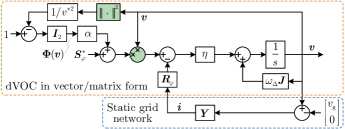
Figure 3: A detailed block diagram of the reduced second-order GFM converter system, where the nonlinear elements are highlighted in green.

III-C Stability Problem Statement

For the full-order and reduced-order systems given in (18) to (21), we aim to explore the following stability problems.

1. Under what conditions do equilibria exist?

2. Under what conditions is an equilibrium globally stable?

3. How will transient instability behave when unstable?

These stability problems are closely relevant to the planning, design, and operation (particularly relevant to fault ride-through and transient operation) of GFM converters, drawing the attention of system planners, system operators, equipment manufacturers, and many researchers. In contrast to the numerical results available in the literature, we provide analytical results and quantitative stability conditions in this study.

Remark 4 (Current limiting issue).

The transient stability of GFM converters is also related to their current limiting strategies [34]. When a grid fault occurs, the grid enters into an abnormal operation stage, during which converters should maintain GFM operation with auxiliary control/protection strategies. Ideally, we expect the converters under grid faults to remain as voltage sources and in the same model form as under normal conditions. This is motivated because, if so, we can apply the same approach in modeling, stability analysis and assessment, and system operation for both fault and non-fault conditions. This is indeed the case for conventional power systems. In another parallel work [35], we have designed a saturation-informed current-limiting strategy applicable for various GFM controls, which is able to recover an equivalent standard GFM control from the current-saturated operating condition under grid faults, achieving the specification above. In this study, we focus on addressing the stability of the standard control form. Our results have been extended to the current-saturated scenario [35].

IV Stability of Second-Order GFM Dynamics

We first study the reduced second-order system in (19) and then extend the results to the full-order system in (18). The main results are outlined in this and the next section to rapidly grasp the whole picture, while technical details are provided comprehensively in Appendices A and B. The technical details not only theoretically consolidate the stability analysis of dVOC but also provide inspiration for the stability analysis of other GFM controls.

IV-A Existence of Equilibrium Points

The existence of equilibria is necessary for achieving stability in a steady state. We prove that equilibrium points of complex droop control always exist, see Proposition 3 in Appendix A for details. In contrast, there exist scenarios in which classical droop control does not admit a steady state, and a counterexample is illustrated in Example 3 in Appendix A. In respect thereof, classical droop control can suffer from transient instability due to the absence of equilibria. Unlike classical droop control, complex droop control does not suffer from this shortage. From the argument in the proof of Proposition 3, we reveal one reason for this is that the power feedback is normalized by the voltage amplitude square. The other reason is that a fixed setpoint for the normalized power is employed, i.e., $\overline{\underline{\varsigma}}^{\star}=(p^{\star}-jq^{\star})/v^{\star 2}$.

IV-B Transient Stability of Complex Droop Control

For a unique equilibrium $\boldsymbol{v}_{\rm s}$, a sufficient condition for global stability is identified by Theorem 7 in Appendix A as

$$\real\{e^{j\varphi}\tfrac{p^{\star}-jq^{\star}}{v^{\star 2}}\bigr{\}}+\alpha<\tfrac{1}{2}\tfrac{\alpha}{v^{\star 2}}\norm{\boldsymbol{v}_{\rm s}}^{2}+\real\{e^{j\varphi}\underline{y}\bigr{\}}.$$ (22)

TABLE III: Parametric Impact on the Stability of Complex Droop Control

Parameter change	Implication	Impact
$\absolutevalue{p^{\star}-jq^{\star}}$ $\uparrow$	Enlarge the magnitude of the power setpoint.	Negative
$\lvert{\underline{y}}\rvert$ $\uparrow$	Reduce the magnitude of the grid impedance.	Positive
$\alpha$ $\uparrow$	Increase the gain of the voltage amplitude regulation.	Mostly negative1
$v_{\rm s}$ or $v_{\rm g}$ $\uparrow$	Raise the voltage level of the system.	Positive
$\cos\bigl(\varphi-\angle\underline{z}\bigr{missing})$ $\uparrow$	Match the rotation angle with the grid impedance angle.	Positive
$\cos\bigl(\varphi-\arctan\frac{q^{\star}}{p^{\star}}\bigr{missing})$ $\uparrow$	Match the rotation angle with the power factor angle setpoint.	Negative

• $\alpha$ appears on both sides of (22), where the steady-state voltage value is also involved.

The condition in (22) relies on the equilibrium point information, which may be unknown. From (22), a tighter condition for global stability can be directly provided without using the equilibrium point information as

$$\real\{e^{j\varphi}\tfrac{p^{\star}-jq^{\star}}{v^{\star 2}}\bigr{\}}+\alpha<\real\{e^{j\varphi}\underline{y}\bigr{\}}.$$ (23)

Remark 5 (Interpretation of the stability conditions).

The stability conditions in (22) and (23) provide quantitative insights into parametric impacts on stability, which are summarized in Table III. The first four pieces of insights are in line with well-known engineering experience. We provide an explanation for the last one. As seen from the model in (19), the real part of $e^{j\varphi}\overline{\underline{\varsigma}}^{\star}$ regulates the $dq$-axis voltages with positive feedback. The match of the rotation angle ($\varphi$) with the power factor angle setpoint ($\arctan\tfrac{q^{\star}}{p^{\star}}$) leads to a large regulation gain, therefore not being conducive to stability. Moreover, we notice that the stability condition in (22) for the grid-connected case resembles that in [19, Condition 3] for the microgrid case.

IV-C Transient Instability as Limit Cycle Oscillations

We prove that the trajectories of complex droop control are always bounded, see Proposition 9. The trajectory boundedness implies that transient instability will manifest as limit cycles (periodic orbits) inside the bound. More precisely, if the trajectories of the system in (19) cannot converge to equilibrium points, then they must converge to limit cycles, cf. Theorem 10 in Appendix A. Moreover, if there is only one equilibrium point and it is unstable, then all the initial states, except for the equilibrium point, converge to limit cycles, cf. Corollary 10.1. The condition for the uniqueness of equilibrium points can be found in Proposition 4, and the condition for an equilibrium point being unstable can be found in Proposition 6. Namely, Propositions 4 and 6 provide sufficient parametric conditions for transient instability.

Remark 6 (Upper bound of the voltage profile).

Under grid disturbances, there exists an upper bound for the converter voltage profile (even in the case of transient instability). The bound, denoted as $v_{\rm m}$, is identified in Proposition 9 as $v_{\rm m}=\max\bigl{\{}v_{\rm g},\,v^{\star}\bigl{(}1+\tfrac{\kappa_{\rm r}+\lvert\underline{y}\rvert}{\alpha}\bigr{)}^{1/2}\bigr{\}}$. We remark that the existence of the upper bound can bring useful insights into the overvoltage protection of converters.

V Stability of Full-Order System Dynamics

This section extends our results from the reduced second-order system to the full-order system. The main focus is exploring the second problem stated in Section III-C, i.e., under what conditions the equilibrium of the full-order system is asymptotically stable either globally or within a wide region of attraction. Concerning the other two problems, the full-order system shares the same equilibria as the reduced-order systems. Moreover, the transient instability of the full-order system, if dominated by the GFM dynamics, still manifests itself as limit cycle oscillations, as shown later in case studies.

To explore the transient stability of the full-order system, we resort to the nested singular perturbation approach developed in [18]. The approach aims to establish a stability guarantee for a nested interconnection of nonlinear dynamic systems ordered from slow to fast, where more than two time scales can be considered, beyond classical singularly perturbed systems [36, Theorem 11.3]. The approach has been applied to study converter-based islanded systems [18]. In this work, we apply it to the grid-connected case, where the grid voltage appears as a forced input, making the stability analysis largely different.

By applying the nested singular perturbation analysis (see Appendix B for details), the following conditions are identified, which bound the controller set-points ($p^{\star}$, $q^{\star}$, $v^{\star}$), grid parameters ($\underline{y}$, $l_{\rm g}$, $r_{\rm g}$), and control parameters ($\alpha$, $\eta$, $\varphi$, ${k_{\rm p}^{\rm v}}$, ${k_{\rm r}^{\rm v}}$, ${k_{\rm p}^{\rm c}}$, ${k_{\rm r}^{\rm c}}$) to ensure the stability of the full-order system, i.e.,

$$\real\{e^{j\varphi}\tfrac{p^{\star}-jq^{\star}}{v^{\star 2}}\bigr{\}}+\alpha+c_{1}<\tfrac{1}{2}\tfrac{\alpha\norm{\boldsymbol{v}_{\rm s}}^{2}}{v^{\star 2}}+\real\{e^{j\varphi}\underline{y}\bigr{\}},$$ (24a)

$$0<\eta<\frac{c_{1}}{\frac{l_{\rm g}}{r_{\rm g}}\norm{\boldsymbol{Y}}(c_{1}+c_{\epsilon})},$$ (24b)

$$0<\frac{1+{k_{\rm r}^{\rm v}}/{k_{\rm p}^{\rm v}}}{{k_{\rm r}^{\rm v}}/{c_{\rm f}}-1}<\frac{4c_{2}}{\frac{1}{r_{\rm g}}\eta(c_{\epsilon}^{2}+4)},$$ (24c)

$$0<\frac{1+{k_{\rm r}^{\rm c}}/{k_{\rm p}^{\rm c}}}{{k_{\rm r}^{\rm c}}/{l_{\rm f}}-1}<\frac{4c_{3}}{\frac{\beta_{34}}{\tilde{\beta}_{43}}(\tilde{\beta}_{41}^{2}+\tilde{\beta}_{42}^{2}+4\tilde{\beta}_{43}^{2})+c_{3}\tilde{\gamma}_{4}},$$ (24d)

where $c_{1}$, $c_{2}$, and $c_{3}$ quantify the stability margins concerning the unfavorable interaction appearing between adjacent time scales of dynamics, and $c_{\epsilon}$ is a tunable quantity related to another tunable parameter $\epsilon$. The definition of all of these parameters/variables can be found in Appendix B.

As a result of the grid voltage forced input in the grid-connected case, the stability conditions in (24) (particularly the first three) differ from those in [18] for islanded systems. However, they maintain similar physical interpretations. Broadly, the first inequality guarantees that the GFM dynamics alone are stable, the second one requires the GFM dynamics to be slow enough compared to the network dynamics, the third one implies that the voltage tracking should be sufficiently fast compared to the network dynamics, and the last one necessitates that the current tracking should be faster than the voltage tracking (see [18, Sec. VI-E] for further discussions). The above result can be also extended to multi-converter grid-connected systems, see our results in [37].

Concerning the reduced fourth-order and eighth-order systems in (20) and (21), their stability conditions can be straightforwardly extracted from those of the full-order system. More precisely, the stability conditions of the former comprise (24a) and (24b), while those of the latter comprise (24a) to (24c).

Remark 7 (Conservatism of the stability conditions).

The conservatism of the stability condition in (24a) can be reflected by one of the instability conditions given in Proposition 6, which reads as $\real\{e^{j\varphi}\tfrac{p^{\star}-jq^{\star}}{v^{\star 2}}\bigr{\}}+\alpha>2\tfrac{\alpha}{v^{\star 2}}\norm{\boldsymbol{v}_{\rm s}}^{2}+\real\{e^{j\varphi}\underline{y}\bigr{\}}$. The only difference in the coefficients $1/2$ and $2$ reveals that a smaller steady-state voltage $\norm{\boldsymbol{v}_{\rm s}}$ implies less conservatism. The conservatism of (24b) is illustrated in Fig. 5 in case studies, where the condition for $\eta$ is conservative around $1/2$ to $1/10$, affected by $\alpha$. Moreover, we have verified that (24c) is easily satisfied. However, (24d) is considerably conservative, requiring unrealistically high current control gains. In spite of this, the quantitative conditions provide valuable parameter tuning guidelines by directing engineers on the relative order and direction of tuning of the cascaded loops.

Remark 8 (Region of attraction).

Different from the global stability guarantee for the second-order system, we only obtain a non-global stability guarantee for the high-order systems. However, the region of attraction can still be guaranteed to be wide enough. Specifically, the region of attraction is given as $\{(\boldsymbol{x}_{1},\boldsymbol{x}_{2},\boldsymbol{x}_{3},\boldsymbol{x}_{4})\,\big{|}\,\norm{\boldsymbol{x}_{1}-\boldsymbol{v}_{\rm s}}<r\}$, reflecting the largest sublevel set of the Lyapunov function $V_{1}$ on the largest neighbourhood $B_{r}\coloneqq\{\boldsymbol{x}_{1}\,\big{|}\,\norm{\boldsymbol{x}_{1}-\boldsymbol{v}_{\rm s}}<r\}$, where $r>0$ is the positive real root of $\frac{(1+r/\norm{\boldsymbol{v}_{\rm s}})^{3}-1}{1/\norm{\boldsymbol{v}_{\rm s}}}=\epsilon$ (see Lemma 12 and illustrative Example 4 in Appendix B for further details). Hence, a larger $\epsilon$ implies a wider region of attraction. On the other hand, a large $\epsilon$ will downsize the control gains in (24) and accordingly slow down the whole dynamic response.

VI Simulation and Experimental Validations

We present case studies to validate our previous theoretical results. First of all, we provide a comparative illustration of transient responses among the systems of different orders in (18) to (21). Afterwards, we compare the analytical parametric stability range and associated simulation results. Thirdly, we validate that the transient instability of complex droop control manifests as limit cycle oscillations. Last, we validate that complex droop control achieves robust stability performance also in the case of non-ideal grid conditions. We remark that the full-order system encompasses all dynamics and thus serves as a high-fidelity model. The system parameters that are identically adopted in all of the case studies are given in the following: $S_{N}=2$ MVA, $V_{N}=690$ V, $f_{N}=50$ Hz, $\omega_{\rm g}=1.0$ pu, $v_{\rm g}=1.0$ pu, $l_{\rm f}=c_{\rm f}=0.05/\omega_{0}$ s/rad, $r_{\rm f}=g_{\rm f}=0.05/30$ pu, $k_{\rm p}^{\rm v}=1$ pu, $k_{\rm r}^{\rm v}=10$ pu/s, $k_{\rm p}^{\rm c}=2$ pu, $k_{\rm r}^{\rm c}=20$ pu/s. The other parameters are adjusted differently in each case study and therefore provided in their respective subsections. The main results are also validated by experimental results based on real hardware converters.

VI-A Case Study I: Transient Response for Different Orders

The following parameters are considered in this case study: $r_{\rm g}=0.08$ pu, $l_{\rm g}=0.2/\omega_{0}$ s/rad, $\varphi=\arctan\frac{l_{\rm g}}{r_{\rm g}}$, $p^{\star}=0.5$ pu, $q^{\star}=0.2$ pu, $v^{\star}=1.0$ pu, $v_{\rm g,dip}=0.5$ pu, and $\alpha=1$ pu. The transient response of the four systems with different orders under a grid voltage dip is depicted in Fig. 4. In Fig. 4(a), a smaller value of $\eta=0.02\omega_{0}$ is employed, which meets the stability condition in (24b). It can be observed that the full-order, eighth-order, and fourth-order systems exhibit similar transient responses. They, however, show deviations from the second-order system during the short period following the grid voltage dip. The deviation occurs due to the transient behaviors of circuit electromagnetic transients and/or inner-loop dynamics. From the result of decay rates, it is seen that the four different time scales of dynamics in the full-order system roughly exhibit a time-scale separation from fast to slow. While the separation among the fast dynamics is not particularly significant, all of them operate at a faster rate compared to the dVOC GFM dynamics. Provided that circuit electromagnetic transients and inner-loop dynamics decay rapidly compared to the GFM dynamics, one may choose to use the second-order system, which only includes the dVOC GFM dynamics, for transient stability analysis.

In Fig. 4(b), a larger value of $\eta=0.06\omega_{0}$ is utilized, which accelerates the dVOC GFM dynamics, violating the stability condition in (24b). Consequently, the GFM dynamics may interfere with the other dynamics. This interference is verified by the decay rate results, where the dVOC dynamics are even faster than the other dynamics. As a result, the electromagnetic dynamics exhibit poor transient characteristics, leading to noticeable oscillations, which take longer to decay. Therefore, in situations of severe interference, the second-order system may inadequately capture the transient response, necessitating the use of higher-order models. We note that similar results have been reported in prior studies pertaining to various GFM control strategies, such as in [38] concerning the interference between classical droop control and network dynamics. Our presented quantitative stability conditions in (24) provide valuable insights for mitigating such interference and offer guidance to engineers for the appropriate tuning of control gains in dVOC-controlled multi-time-scale converter systems. The following case study demonstrates that there exists an upper bound for $\eta$ to prevent the adverse interference between GFM dynamics and network dynamics.

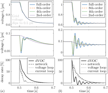
Figure 4: Transient response of systems of different orders. (a) $\eta=0.02\omega_{0}$ rad/s, (b) $\eta=0.06\omega_{0}$ rad/s. The decay rate of different time scales of dynamics in the full-order system is represented by the error coordinates (normalized by their maximums): $\norm{\hat{\boldsymbol{v}}-\boldsymbol{v}_{\rm s}}/\norm{\hat{\boldsymbol{v}}-\boldsymbol{v}_{\rm s}}_{\max}$, $\norm{\boldsymbol{y}_{2}}/\norm{\boldsymbol{y}_{2}}_{\max}$, $\norm{\boldsymbol{y}_{3}}/\norm{\boldsymbol{y}_{3}}_{\max}$, and $\norm{\boldsymbol{y}_{4}}/\norm{\boldsymbol{y}_{4}}_{\max}$, see (53) in Appendix B for the definition of the error coordinates $\boldsymbol{y}_{i}$, $i\in\{2,3,4\}$.

VI-B Case Study II: Parametric Stability Range

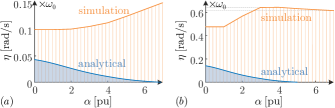
Figure 5: Comparison of the parametric stability ranges between the analytical result in (24a) and (24b) and the precise result by simulations traversing the parameter space. (a) $r_{\rm g}=0.08$ pu and (b) $r_{\rm g}=0.20$ pu.

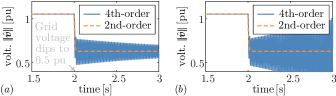
Figure 6: Concerning the critical stable case $(\alpha=1,\eta=0.100\omega_{0})$ in Fig. 5(a), the 4th-order system in (20) is stable with $\eta=0.099\omega_{0}$ in (a), whereas it is unstable with $\eta=0.101\omega_{0}$ in (b).

We consider the reduced fourth-order system with stability conditions in (24a) and (24b) as an example, where two control gains of complex droop control, i.e., $\eta$ and $\alpha$, are constrained. We use the same parameters as in Section VI-A to exemplify the parametric stability range in terms of $\eta$ and $\alpha$.

The boundary of the analytical stability conditions in (24a) and (24b) is plotted by fixing a value of $\alpha$, solving the equilibrium, and finding the upper bound of $\eta$, as shown in Fig. 5. The precise boundary is identified via simulations by traversing the parameter space. It can be seen that the analytical boundary is located strictly within the precise boundary as expected since the analytical results are sufficient but not necessary. By comparison between Fig. 5(a) and (b), we remark that a larger $r_{\rm g}$ leads to a smaller time constant (faster decay) of the network dynamics, $\frac{l_{\rm g}}{r_{\rm g}}$, which allows a larger $\eta$, i.e., faster GFM dynamics. Moreover, it is verified by the precise boundary in Fig. 5(b) that the impact of $\alpha$ on stability is not entirely negative, cf. the result in Table III, since the boundary is non-monotonically growing.

Consider a critical stable case, where $\alpha=1$, $\eta=0.100\omega_{0}$ in Fig. 5(a). It is observed from the simulation result in Fig. 6 that a larger $\eta$ immediately results in instability of the fourth-order system whereas a smaller $\eta$ can maintain stability. The second-order system, however, remains stable in both results. This is due to the fact that $\eta$ is not bounded in the stability condition (22) for the second-order system. This suggests again that $\eta$ should not be overly large (the GFM dynamics should not be too fast) in the presence of network dynamics.

VI-C Case Study III: Transient Instability as Limit Cycles

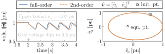
Figure 7: Transient instability of the complex-droop-controlled converter system behaves as a time-domain periodic oscillation or a phase-plane limit cycle.

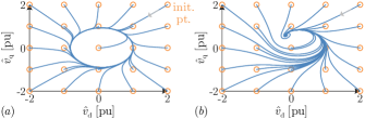
Figure 8: The complex-droop-controlled converter system (2nd-order) converges either to a limit cycle in (a), where $\alpha=3$ pu, or to an equilibrium point in (b), where $\alpha=1$ pu, from any non-equilibrium initial points.

The transient instability of complex droop control, if dominated by GFM dynamics, will manifest as periodic oscillations, since the second-order GFM dynamic trajectories are proved to be bounded. We consider the following parameters to illustrate the transient instability response: $r_{\rm g}=0.8$ pu, $l_{\rm g}=0.8/\omega_{0}$ s/rad, $\varphi=\arctan\frac{l_{\rm g}}{r_{\rm g}}$, $\eta=0.08\omega_{0}$ rad/s, $\alpha=3$ pu, $p^{\star}=0.8$ pu, $q^{\star}=-0.2$ pu, $v^{\star}=1.0$ pu, $v_{\rm g,dip}=0.5$ pu. By Proposition 4, it is identified that the system has a unique equilibrium. By Proposition 6, it is identified that the equilibrium is unstable. Therefore, it follows from Corollary 10.1 that all the initial states of the GFM dynamics, except for the equilibrium point, converge to a limit cycle.

As seen in Fig. 7, both the full- and second-order systems result in transient instability display limit cycle oscillations. The full-order system response is very close to the second-order one, implying that the instability is dominated by the GFM dynamics. Moreover, it is observed that the transient trajectory lies under the upper bound we identified, cf. Remark 6, which suggests that the converter is free of overvoltage beyond the upper bound. To further observe the transient response of the GFM dynamics initiating from different initial points, we provide the phase plane plots in Fig. 8. In Fig. 8(a), all the trajectories converge to the limit cycle. If we reduce $\alpha$ from $3$ to $1$, then a stable equilibrium point will be generated. Fig. 8(b) shows that the GFM dynamics are stable in this case, as opposed to the transient instability in Fig. 8(a), and the trajectories from all the initial points converge to the equilibrium point. For this stable case, however, we verified that the sufficient stability condition in (22) is not satisfied. This can be justified because the system admits a larger parametric stability range than our analytical result, as illustrated in Fig. 5.

VI-D Case Study IV: Robust Transient Response

The robust stability performance of complex droop control is also crucial in practice, where the power grid is not an infinite bus. We use a prototypical system in Fig. 9 to validate that complex droop control can achieve robust transient stability performance in a grid of synchronous generators. The system consists of a complex-droop-controlled converter, a synchronous generator, and a constant impedance load. The parameters are given as $r_{\rm c}=0.06$ pu, $l_{\rm c}=0.30$ pu, $r_{\rm g}=0.01$ pu, $l_{\rm g}=0.05$ pu, $r_{\rm load}=0.8$ pu, $l_{\rm load}=1.2$ pu, $r_{\rm fault}=0.01\ \Omega$, $\varphi=\arctan\frac{l_{\rm c}}{r_{\rm c}}$, $\eta=0.03\omega_{0}$ rad/s, $\alpha=3$ pu, $p^{\star}=0.6$ pu, $q^{\star}=0.2$ pu, $v^{\star}=1.0$ pu. The generator capacity is ten times the converter capacity, with the main parameters given as $x_{\rm d}^{\prime}=0.17$ pu, $r_{\rm s}=0.038$ pu, $t_{\rm d}^{\prime}=2.03$ s, $H=4$ s, $R_{\rm g}=0.03$ pu, $p_{\rm m}=0.3$ pu.

Figure 9: A GFM converter is connected to a non-ideal grid represented by a synchronous generator.

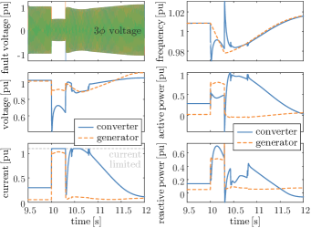
Figure 10: In a non-ideal grid scenario, the complex-droop-controlled GFM converter can also achieve transient stability during a grid fault.

A three-phase short-circuit fault occurs on the load bus at $10$ s. Then, the generator frequency drops down slowly since it supplies high active power under the fast action of a fast excitation system. The converter is configured with a saturation-informed current-limiting strategy [35], which limits the converter output current while maintaining dVOC’s synchronizing and regulating capabilities. Consequently, the converter almost achieves synchronization with the generator during the grid fault, and it supplies increased reactive power to support voltage. After the fault is cleared at $10.3$ s, the system maintains synchronization and transient stability, slowly settles down in the original steady state, and preserves power sharing between the converter and the generator.

VI-E Experimental Results

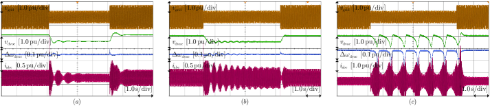
Figure 11: Experimental results indicate that the stability of dVOC (i.e., complex droop control) deteriorates with the increase of the voltage regulation gain $\alpha$, and the instability of dVOC exhibits periodic oscillation. (a) $\alpha=0$. (b) $\alpha=1$. (c) $\alpha=2$. The signal $v_{\mathrm{grid}}$ represents the grid voltage, $v_{\mathrm{dvoc}}$ and $\omega_{\mathrm{dvoc}}$ represent the control output of dVOC, and $i_{\mathrm{abc}}$ represent the output current of inverter I.

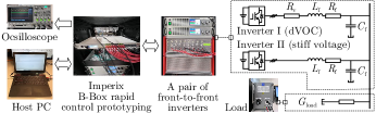
Figure 12: Experimental setup, where the nominal power capacity is $2$ kVA, the phase-to-phase RMS nominal voltage is $300$ V, and the filter parameters are as follows: $L_{\mathrm{f}}=1.5$ mH, $R_{\mathrm{f}}=1.0$ $\Omega$, and $C_{\mathrm{f}}=3.5$ $\mu$F.

The experimental setup depicted in Fig. 12 is used to further validate the theoretical results. It involves the interconnection of two inverters in a front-to-front configuration, with one employing complex droop control and the other emulating a stiff grid. A virtual resistive line impedance $R_{\mathrm{v}}$ is implemented in inverter I (although it may also be implemented in inverter II) to enable the manipulation of the grid connection strength. The power generated by the inverters is then directed to a resistive load. Both inverters are controlled by an Imperix B-Box rapid control prototyping (RCP) system, which employs a dual-core ARM processor for the execution of control algorithms. The control code is compiled from a Simulink control model residing on the host computer. The RCP system supports real-time debugging and monitoring, allowing us to adjust control parameters online as well as capture signal waveforms through an oscilloscope. The PWM switching frequency is $32$ kHz, and the sampling and control frequency is $8$ kHz. It is noteworthy that the complex droop control in polar coordinates, instead of the dVOC in $\alpha\beta$ coordinates, is implemented in the control algorithm. In the case of choosing the dVOC, a higher control frequency may be required to ensure control accuracy, given the involvement of the integration of sinusoidal signals.

The experiments incorporate the following main parameters: $R_{\rm v}=0.2$ pu, $G_{\mathrm{load}}=0.56$ pu, $\varphi=\pi/2$, $p^{\star}=0.3$ pu, $q^{\star}=0.0$ pu, $v^{\star}=1.0$ pu, $v_{\rm g,dip}=0.5$ pu, and $\alpha\in\{0,1,2\}$ pu. The transient response of the system under the grid voltage dip to $v_{\rm g,dip}$ is shown in Fig. 11. Notably, the system approaches marginal stability during the grid voltage dip, primarily due to the mismatch between the setting of $\varphi$ and the predominantly resistive network characteristic. Specifically, the system maintains transient stability with $\alpha=0$ or $1$ while instability is observed with $\alpha=2$. This observation is consistent with the theoretical results, indicating that the mismatch of $\varphi$ with the network impedance angle as well as the increase in $\alpha$ contributes to the deterioration of dVOC stability. Moreover, it is observed from Fig. 11(c) that the transient instability manifests as periodic oscillation, consistent with the theoretical results. We notice that the inverter output current exhibits high spikes during transients or instability, while both inverters still remain operating, which is because the nominal capacity is reduced for safety compared to the actual capacity. In our upcoming studies, we will assess the current limiting performance and transient stability of grid-forming controls under grid faults [35].

VII Conclusion

We have investigated the transient stability of complex droop control (i.e., dVOC) in grid-forming converters connected to power grids. We prove that complex droop control achieves transient stability explicitly under the quantitative stability conditions we derived, demonstrating its superiority over classical droop control. The transient stability of complex droop control, in the multi-time-scale full-order dynamic system, also remains guaranteed within a wide region of attraction. The transient instability of complex droop control is shown to be bounded, manifesting itself as limit cycle oscillations. Our derived analytical stability/instability conditions and identified trajectory upper bound provide theoretical insights for practical parameter tuning, stability certificating, and stable operation of grid-forming converters. In another parallel work, we explore a saturation-informed feedback control to address the current limiting issue in grid-forming converters, where the stability results of the standard grid-forming control have been extended to guarantee transient stability under current saturation. Moreover, the transient stability of converter and generator mixed systems is part of our future research.

Appendix A Stability Results of the Second-Order System

We first provide two degenerated examples of the reduced second-order system and present their stability results.

Example 1 (Voltage-following mode).

As mentioned in Section II-B, if $\alpha=0$ is employed, the GFM control will degenerate into a voltage-following one. Then, the model in (19) reduces to

$$\dot{{\boldsymbol{v}}}=[\omega_{\Delta}\boldsymbol{J}+\eta(\boldsymbol{S}_{\varphi}^{\star}-\boldsymbol{Y}_{\varphi})]{\boldsymbol{v}}+\eta\boldsymbol{Y}_{\varphi}\boldsymbol{v}_{\rm g}.$$ (25)

The dynamics in (25) are linear, and the stability analysis, in this case, is trivial, and provided in Proposition 1. We highlight that this voltage-following control mode proves to be globally stable and also naturally supports the grid frequency in a droop fashion, by contrast to classical grid-following control by phase-locked loops (PLLs) [39]. Moreover, it is linear and thus tractable from the analysis point of view.

Proposition 1.

Consider the linear system in (25) (i.e., $\alpha=0$). The system is globally asymptotically stable if and only if

$$\real\{e^{j\varphi}\tfrac{p^{\star}-jq^{\star}}{v^{\star 2}}\bigr{\}}<\real\{e^{j\varphi}\underline{y}\bigr{\}}.$$ (26)

The system matrix in (25), i.e., $[\omega_{\Delta}\boldsymbol{J}+\eta(\boldsymbol{S}_{\varphi}^{\star}-\boldsymbol{Y}_{\varphi})]$, is Hurwitz if and only if $\Re{e^{j\varphi}(\overline{\underline{\varsigma}}^{\star}-\underline{y})}<0$.

Example 2 (Off-grid mode).

Consider the other particular case where $\boldsymbol{v}_{\rm g}=\mathbbb{0}_{2}$ while $\alpha\neq 0$. This case means that the converter is off-grid/islanded to feed a constant impedance load. Accordingly, the model in (19) becomes

$$\dot{{\boldsymbol{v}}}=[\omega_{\Delta}\boldsymbol{J}+\eta(\boldsymbol{S}_{\varphi}^{\star}-\boldsymbol{Y}_{\varphi})+\eta\alpha\boldsymbol{I}_{2}]{\boldsymbol{v}}-\tfrac{\eta\alpha}{v^{\star 2}}\norm{\boldsymbol{v}}^{2}{\boldsymbol{v}}.$$ (27)

It is interesting to notice that the off-grid GFM dynamics in (27) follow the norm form of the Andronov-Hopf oscillator (also known as the Stuart-Landau oscillator) [40], i.e.,

$$\dot{\underline{z}}=\underline{\mu}\underline{z}-\underline{\xi}\absolutevalue{\underline{z}}^{2}\underline{z},$$ (28)

with gains $\underline{\xi}$, $\underline{\mu}\in\mathbb{C}$ and the state of the oscillator $\underline{z}\in\mathbb{C}$. The stability analysis of a single Andronov-Hopf oscillator is trivial and already available in [40]. The stability result of (27) is directly provided in the following.

Proposition 2.

The system in (27) (i.e., $\boldsymbol{v}_{\rm g}=\mathbbb{0}_{2}$) is globally asymptotically stable w.r.t the origin if and only if

$$\real\{e^{j\varphi}\tfrac{p^{\star}-jq^{\star}}{v^{\star 2}}\bigr{\}}+\alpha\leq\real\{e^{j\varphi}\underline{y}\bigr{\}}.$$ (29)

Otherwise, there exists a circular limit cycle, the amplitude square of which is $\norm{\boldsymbol{v}}^{2}=\tfrac{v^{\star 2}}{\alpha}\Bigl{(}\real\{e^{j\varphi}\tfrac{p^{\star}-jq^{\star}}{v^{\star 2}}-e^{j\varphi}\underline{y}\bigr{\}}+\alpha\Bigr{)}$.

Consider the norm form of the Stuart-Landau oscillator in (28). It has been shown in [40, Theorem 1] that if $\real\{\underline{\mu}\}\leq 0$, then the origin is globally asymptotically stable, while if $\real\{\underline{\mu}\}>0$, then the limit cycle $\bigl{\{}\lvert\underline{z}\rvert^{2}=\real\{\underline{\mu}\}/\real\{\underline{\xi}\}\bigr{\}}$ is globally asymptotically stable for all initial states except for the origin. We apply this result to the system in (27), which completes the proof.

From now on, we consider the general case for the second-order system in (19), where $\alpha\neq 0$ and $\boldsymbol{v}_{\rm g}\neq\mathbbb{0}_{2}$. In the general case, since $\boldsymbol{v}_{\rm g}$ plays as a forced input, the stability analysis becomes non-trivial. The stability analysis for this forced system is one of our theoretical contributions.

A-A Existence, Uniqueness, and Local Stability of Equilibria

Proposition 3.

The GFM converter system in (19) with complex droop control always has equilibrium points. In contrast, the GFM converter system with the classical droop control in (6) or with VSM does not always have an equilibrium point.

To render the steady-state equation for complex droop control comparable to that for classical droop control, we consider both models in polar coordinates. For complex droop control in a steady state, we have, cf. (10), that

$$0 =\eta\left(\sigma_{\varphi}^{\star}-\sigma_{\varphi\rm s}\right)+\eta\alpha\left({v^{\star 2}-v_{\rm s}^{2}}\right)/{v^{\star 2}},$$ (30a)

$$0 =\omega_{\Delta}+\eta\left(\rho_{\varphi}^{\star}-\rho_{\varphi\rm s}\right),$$ (30b)

where the subscript ${\rm s}$ denotes steady-state variables (the same hereinafter). From (11b), the rotated power is given as $\sigma_{\varphi\rm s}+j\rho_{\varphi\rm s}=e^{j\varphi}\overline{\underline{\varsigma}}_{\rm s}=e^{j\varphi}(p_{\rm s}-jq_{\rm s})/{v_{\rm s}^{2}}$. Given that

$$p_{\rm s} =v_{\rm s}^{2}\lvert\underline{y}\rvert\cos{(\angle{\underline{z}})}-v_{\rm g}v_{\rm s}\lvert\underline{y}\rvert\cos\left(\delta_{\rm s}+\angle{\underline{z}}\right),$$ (31a)

$$q_{\rm s} =v_{\rm s}^{2}\lvert\underline{y}\rvert\sin{(\angle{\underline{z}})}-v_{\rm g}v_{\rm s}\lvert\underline{y}\rvert\sin\left(\delta_{\rm s}+\angle{\underline{z}}\right),$$ (31b)

it follows that

$$\sigma_{\varphi\rm s} =\lvert\underline{y}\rvert\cos{\phi}-v_{\rm g}\lvert\underline{y}\rvert\cos\left(\delta_{\rm s}+\phi\right)/v_{\rm s},$$ (32a)

$$\rho_{\varphi\rm s} =-\lvert\underline{y}\rvert\sin{\phi}+v_{\rm g}\lvert\underline{y}\rvert\sin\left(\delta_{\rm s}+\phi\right)/v_{\rm s}.$$ (32b)

where $\phi\coloneqq\angle{\underline{z}}-\varphi$ denotes the rotated grid-impedance angle, and $\delta_{\rm s}$ denotes the steady state of $\delta\coloneqq\theta-\theta_{\rm g}$.

Then, it follows by substituting (32) into (30) that

$$\sigma_{\varphi}^{\star}+\alpha-\alpha\tfrac{v_{\rm s}^{2}}{v^{\star 2}} =\lvert\underline{y}\rvert\cos{\phi}-v_{\rm g}\lvert\underline{y}\rvert\cos\left(\delta_{\rm s}+\phi\right)/v_{\rm s},$$ (33a)

$$\rho_{\varphi}^{\star}+\tfrac{\omega_{\Delta}}{\eta} =-\lvert\underline{y}\rvert\sin{\phi}+v_{\rm g}\lvert\underline{y}\rvert\sin\left(\delta_{\rm s}+\phi\right)/v_{\rm s},$$ (33b)

where there are two unknown variables $v_{\rm s}$ and $\delta_{\rm s}$. By eliminating $\delta_{\rm s}$, we obtain that

$$\bigl{[}\sigma_{\varphi}^{\star}+\alpha-\alpha\tfrac{v_{\rm s}^{2}}{v^{\star 2}}-\lvert\underline{y}\rvert\cos{\phi}\bigr{]}^{2}+\bigl{[}\rho_{\varphi}^{\star}+\tfrac{\omega_{\Delta}}{\eta}+\lvert\underline{y}\rvert\sin{\phi}\bigr{]}^{2}=\tfrac{v_{\rm g}^{2}\lvert\underline{y}\rvert^{2}}{v_{\rm s}^{2}}.$$ (34)

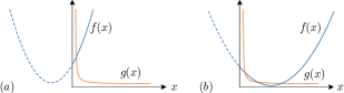
Figure 13: Equation (35) always has positive real roots, i.e., intersections between $f(x)$ and $g(x)$ in the first quadrant. (a) A unique positive real root. (b) At most three real positive roots.

To look into the positive real root of (34) for $v_{\rm s}^{2}$, we substitute $x\coloneqq v_{\rm s}^{2}\in\mathbb{R}_{>0}$ and rewrite (34) as

$$\underbrace{\bigl{[}\sigma_{\varphi}^{\star}+\alpha-\alpha\tfrac{x}{v^{\star 2}}-\lvert\underline{y}\rvert\cos{\phi}\bigr{]}^{2}+\bigl{[}\rho_{\varphi}^{\star}+\tfrac{\omega_{\Delta}}{\eta}+\lvert\underline{y}\rvert\sin{\phi}\bigr{]}^{2}}_{f(x),\,x\in\mathbb{R}_{>0}}\\ =\underbrace{\tfrac{v_{\rm g}^{2}\lvert\underline{y}\rvert^{2}}{x}}_{g(x),\,x\in\mathbb{R}_{>0}}.$$ (35)

The left-hand side represents a parabola $f(x)$ opening upwards while the right-hand side represents a hyperbola branch $g(x)$ in the first quadrant. Since $f(x)\geq 0$, the equation (35) can only have positive real roots. As geometrically shown in Fig. 13, in the first quadrant, there must exist at least one intersection between $f(x)$ and $g(x)$. This is true because $\lim_{x\to 0}f(x)-g(x)=-\infty$ while $\lim_{x\to\infty}f(x)-g(x)=\infty$. Once a root for $x$ is solved from (35) (the root can be non-unique), we then choose $v_{\rm s}=\sqrt{x}$, since a positive voltage value is proper.

Given a solution of $v_{\rm s}$, we then use it to solve for $\delta_{\rm s}$ via (33). Both the values of $\cos\left(\delta_{\rm s}+\phi\right)$ and $\sin\left(\delta_{\rm s}+\phi\right)$ are determined by applying the value of $v_{\rm s}$. Thus, there is only one unique solution for $\delta_{\rm s}+\phi$ within a periodic range $[\phi,\,2\pi+\phi)$. Namely, one solution of $v_{\rm s}$ corresponds to one solution of $\delta_{\rm s}$ within $[0,\,2\pi)$. The proof that complex droop control always has equilibrium points is now completed.

For classical droop control, VSM, or their variants, in a steady state, it holds that

$$0 =\eta\left(q_{\varphi}^{\star}-q_{\varphi\rm s}\right)+\eta\alpha\left({v^{\star}-v_{\rm s}}\right),$$ (36a)

$$0 =\omega_{\Delta}+\eta\left(p_{\varphi}^{\star}-p_{\varphi\rm s}\right).$$ (36b)

where the rotated power is referenced from (32) as

$$q_{\varphi\rm s} =\sigma_{\varphi\rm s}v_{\rm s}^{2}=v_{\rm s}^{2}\lvert\underline{y}\rvert\cos{\phi}-v_{\rm s}v_{\rm g}\lvert\underline{y}\rvert\cos\left(\delta_{\rm s}+\phi\right),$$ (37a)

$$p_{\varphi\rm s} =\rho_{\varphi\rm s}v_{\rm s}^{2}=-v_{\rm s}^{2}\lvert\underline{y}\rvert\sin{\phi}+v_{\rm s}v_{\rm g}\lvert\underline{y}\rvert\sin\left(\delta_{\rm s}+\phi\right).$$ (37b)

Similarly, it follows by substituting (37) into (36) and further eliminating $\delta_{\rm s}$ that

$$\bigl{[}q_{\varphi}^{\star}+\alpha v^{\star}-\alpha v_{\rm s}-v_{\rm s}^{2}\lvert\underline{y}\rvert\cos{\phi}\bigr{]}^{2}+\\ \bigl{[}p_{\varphi}^{\star}+\tfrac{\omega_{\Delta}}{\eta}+v_{\rm s}^{2}\lvert\underline{y}\rvert\sin{\phi}\bigr{]}^{2}=v_{\rm g}^{2}\lvert\underline{y}\rvert^{2}v_{\rm s}^{2},$$ (38)

which is a quartic equation regarding $v_{\rm s}$. An arbitrary quartic equation does not necessarily have real roots, not to mention that we require positive real roots for $v_{\rm s}$. It is not hard to find a counterexample, where (38) has no positive real roots, see Example 3. This completes the proof.

Example 3 (Classical droop control lacks an equilibrium point).

The steady-state equation in (38) has no real roots for $v_{\rm s}$ in the following case: $q_{\varphi}^{\star}=0$ pu, $\alpha=1$ pu, $v^{\star}=1$ pu, $\varphi=\pi/2$, $p_{\varphi}^{\star}=0$, $\omega_{\Delta}=0$, $\eta=0.08\omega_{0}$ rad/s, $v_{\rm g}=0.1$ pu, $r_{\rm g}=0.4$ pu, and $l_{\rm g}=0.4$ pu, which can be verified numerically. This example implies that classical droop control may lose the existence of equilibrium points when the grid voltage is far away from $1.0$ pu. However, this violates the default assumption of classical droop control, that is, it is only expected to work around the nominal operating point. One can identify the analytical conditions for the existence of equilibrium points from the quartic equation (38).

There exists at most three equilibria in the complex-droop-controlled converter system in (19), as graphically demonstrated in Fig. 13. To yield global asymptotic stability, we require equilibria to be unique. The conditions for the uniqueness of equilibria are provided in the following.

Proposition 4.

The equilibrium point of the system (19) is unique if and only if the discriminant of the cubic equation from (35), i.e., $ax^{3}+bx^{2}+cx+d=0$, satisfies

$$\Delta\coloneqq b^{2}c^{2}-4ac^{3}-4db^{3}-27a^{2}d^{2}+18abcd<0,$$ (39)

where the coefficients are given as $a\coloneqq{\alpha^{2}}/{v^{\star 4}}$, $b\coloneqq-2{\alpha}\bigl{(}\sigma_{\varphi}^{\star}+\alpha-\tfrac{\alpha}{v^{\star 2}}-\lvert\underline{y}\rvert\cos{\phi}\bigr{)}/{v^{\star 2}}$, $c\coloneqq\bigl{[}\sigma_{\varphi}^{\star}+\alpha-\lvert\underline{y}\rvert\cos{\phi}\bigr{]}^{2}+\bigl{[}\rho_{\varphi}^{\star}+\tfrac{\omega_{\Delta}}{\eta}+\lvert\underline{y}\rvert\sin{\phi}\bigr{]}^{2}$, and $d\coloneqq-v_{\rm g}^{2}\lvert\underline{y}\rvert^{2}$.

A cubic equation has a unique real root if and only if $\Delta<0$. Since we have shown in the proof of Proposition 3 that the equation (35) has only positive real roots, $\Delta<0$ serves as a necessary and sufficient condition for the uniqueness of a positive real root.

Proposition 5.

Consider an equilibrium point $\boldsymbol{v}_{\rm s}$ of the system (19). The equilibrium point is locally asymptotically stable if it holds that

$$\real\{e^{j\varphi}\tfrac{p^{\star}-jq^{\star}}{v^{\star 2}}\bigr{\}}+\alpha<\tfrac{\alpha}{v^{\star 2}}\norm{\boldsymbol{v}_{\rm s}}^{2}+\real\{e^{j\varphi}\underline{y}\bigr{\}}.$$ (40)

The Jacobian matrix of the system (19) at the equilibrium point $\boldsymbol{v}_{\rm s}\coloneqq[v_{\rm ds}\enspace v_{\rm qs}]^{\mathsf{T}}$ is derived as

$$\boldsymbol{A}\coloneqq\begin{bmatrix}\eta\kappa_{\rm r}+\eta\alpha-\eta\alpha\tfrac{3v_{\rm ds}^{2}+v_{\rm qs}^{2}}{v^{\star 2}}&-\omega_{\Delta}-\eta\kappa_{\rm i}-\eta\alpha\tfrac{2v_{\rm ds}v_{\rm qs}}{v^{\star 2}}\\ \omega_{\Delta}+\eta\kappa_{\rm i}-\eta\alpha\tfrac{2v_{\rm ds}v_{\rm qs}}{v^{\star 2}}&\eta\kappa_{\rm r}+\eta\alpha-\eta\alpha\tfrac{3v_{\rm qs}^{2}+v_{\rm ds}^{2}}{v^{\star 2}}\end{bmatrix}.$$

The characteristic equation is then given as

$${\lambda}^{2}+2\eta\bigl{(}\tfrac{2\alpha\norm{\boldsymbol{v}_{\rm s}}^{2}}{v^{\star 2}}-\alpha-\kappa_{\rm r}\bigr{)}{\lambda}\,+$$ (41)

$$\qquad\bigl{(}\kappa_{\rm r}+\alpha-\tfrac{2\alpha\norm{\boldsymbol{v}_{\rm s}}^{2}}{v^{\star 2}}\bigr{)}^{2}-\bigl{(}\tfrac{\alpha\norm{\boldsymbol{v}_{\rm s}}^{2}}{v^{\star 2}}\bigr{)}^{2}+\bigl{(}\tfrac{\omega_{\Delta}}{\eta}+\kappa_{\rm i}\bigr{)}^{2}=0.$$

The equilibrium point is asymptotically stable if it holds that

$$\left\{\begin{aligned} &\kappa_{\rm r}+\alpha<\tfrac{2\alpha\norm{\boldsymbol{v}_{\rm s}}^{2}}{v^{\star 2}},\\ &\bigl{(}\kappa_{\rm r}+\alpha-\tfrac{2\alpha\norm{\boldsymbol{v}_{\rm s}}^{2}}{v^{\star 2}}\bigr{)}^{2}+\bigl{(}\tfrac{\omega_{\Delta}}{\eta}+\kappa_{\rm i}\bigr{)}^{2}>\bigl{(}\tfrac{\alpha\norm{\boldsymbol{v}_{\rm s}}^{2}}{v^{\star 2}}\bigr{)}^{2}.\end{aligned}\right.$$ (42)

A sufficient condition for (42) is $\kappa_{\rm r}+\alpha<\tfrac{\alpha}{v^{\star 2}}\norm{\boldsymbol{v}_{\rm s}}^{2}$, that is $\real\{e^{j\varphi}\tfrac{p^{\star}-jq^{\star}}{v^{\star 2}}\bigr{\}}+\alpha<\tfrac{\alpha}{v^{\star 2}}\norm{\boldsymbol{v}_{\rm s}}^{2}+\real\{e^{j\varphi}\underline{y}\bigr{\}}$, by recalling the definition of $\kappa_{\rm r}$ in Table II. This completes the proof.

Proposition 6.

Consider an equilibrium point $\boldsymbol{v}_{\rm s}$ of the system (19). The equilibrium point is unstable if $\kappa_{\rm r}+\alpha>\tfrac{2\alpha\norm{\boldsymbol{v}_{\rm s}}^{2}}{v^{\star 2}}$ or $\bigl{(}\kappa_{\rm r}+\alpha-\tfrac{2\alpha\norm{\boldsymbol{v}_{\rm s}}^{2}}{v^{\star 2}}\bigr{)}^{2}+\bigl{(}\tfrac{\omega_{\Delta}}{\eta}+\kappa_{\rm i}\bigr{)}^{2}<\bigl{(}\tfrac{\alpha\norm{\boldsymbol{v}_{\rm s}}^{2}}{v^{\star 2}}\bigr{)}^{2}$ holds.

This proposition holds by directly referring to (42).

A-B Global Asymptotic Stability of an Equilibrium Point

Theorem 7.

Assume that the system (19) has a unique equilibrium point $\boldsymbol{v}_{\rm s}$. The equilibrium point is globally asymptotically stable if it holds that

$$\real\{e^{j\varphi}\tfrac{p^{\star}-jq^{\star}}{v^{\star 2}}\bigr{\}}+\alpha<\tfrac{1}{2}\tfrac{\alpha}{v^{\star 2}}\norm{\boldsymbol{v}_{\rm s}}^{2}+\real\{e^{j\varphi}\underline{y}\bigr{\}}.$$ (43)

We define a positive-definite and radially unbounded Lyapunov candidate function w.r.t. $\boldsymbol{v}_{\rm s}$ as

$$V\coloneqq\tfrac{1}{2\eta}\left(\boldsymbol{v}-\boldsymbol{v}_{\rm s}\right)^{\mathsf{T}}\left(\boldsymbol{v}-\boldsymbol{v}_{\rm s}\right),$$ (44)

where $\boldsymbol{v}_{\rm s}$, as a unique equilibrium point, exclusively satisfies the steady-state equation of (19) as

$$\boldsymbol{Y}_{\varphi}\boldsymbol{v}_{\rm g}=-[\tfrac{\omega_{\Delta}\boldsymbol{J}}{\eta}+(\boldsymbol{S}_{\varphi}^{\star}-\boldsymbol{Y}_{\varphi})]{\boldsymbol{v}_{\rm s}}-\alpha\boldsymbol{\Phi}(\boldsymbol{v}_{\rm s}){\boldsymbol{v}_{\rm s}}.$$ (45)

The time derivative of $V$ along the system dynamics in (19) is derived as follows,

$${\dot{V}} = \ \tfrac{1}{\eta}\left(\boldsymbol{v}-\boldsymbol{v}_{\rm s}\right)^{\mathsf{T}}\dot{\boldsymbol{v}}$$

$$= \ \left(\boldsymbol{v}-\boldsymbol{v}_{\rm s}\right)^{\mathsf{T}}\bigl{\{}[\tfrac{\omega_{\Delta}}{\eta}\boldsymbol{J}+(\boldsymbol{S}_{\varphi}^{\star}-\boldsymbol{Y}_{\varphi})]{\boldsymbol{v}}+\boldsymbol{Y}_{\varphi}\boldsymbol{v}_{\rm g}+\alpha\boldsymbol{\Phi}(\boldsymbol{v}){\boldsymbol{v}}\bigr{\}}$$

$$= \ \left(\boldsymbol{v}-\boldsymbol{v}_{\rm s}\right)^{\mathsf{T}}[\tfrac{\omega_{\Delta}}{\eta}\boldsymbol{J}+(\boldsymbol{S}_{\varphi}^{\star}-\boldsymbol{Y}_{\varphi})+\alpha\boldsymbol{I}_{2}]\left(\boldsymbol{v}-\boldsymbol{v}_{\rm s}\right)$$

$$\ -\alpha\tfrac{1}{v^{\star 2}}[\left(\boldsymbol{v}-\boldsymbol{v}_{\rm s}\right)^{\mathsf{T}}(\norm{\boldsymbol{v}}^{2}\boldsymbol{v}-\norm{\boldsymbol{v}_{\rm s}}^{2}\boldsymbol{v}_{\rm s})]$$

$$= \ (\kappa_{\rm r}+\alpha)\left(\boldsymbol{v}-\boldsymbol{v}_{\rm s}\right)^{\mathsf{T}}\left(\boldsymbol{v}-\boldsymbol{v}_{\rm s}\right)$$

$$\ -\alpha\tfrac{1}{v^{\star 2}}[\left(\boldsymbol{v}-\boldsymbol{v}_{\rm s}\right)^{\mathsf{T}}(\norm{\boldsymbol{v}}^{2}\boldsymbol{v}-\norm{\boldsymbol{v}_{\rm s}}^{2}\boldsymbol{v}_{\rm s})]$$

$$\leq \ (\kappa_{\rm r}+\alpha-\alpha\tfrac{1}{v^{\star 2}}\tfrac{1}{2}\norm{\boldsymbol{v}_{\rm s}}^{2})\left(\boldsymbol{v}-\boldsymbol{v}_{\rm s}\right)^{\mathsf{T}}\left(\boldsymbol{v}-\boldsymbol{v}_{\rm s}\right),$$

where the last inequality holds due to Proposition 8. It follows that $\dot{V}$ is negative definite w.r.t. $\boldsymbol{v}_{\rm s}$, if it holds that $\kappa_{\rm r}+\alpha<\tfrac{1}{2}\tfrac{\alpha}{v^{\star 2}}\norm{\boldsymbol{v}_{\rm s}}^{2}$, which is equivalent to (43) by recalling the definition of $\kappa_{\rm r}$ in Table II. This completes the proof.

In this theorem, we require the uniqueness of the equilibrium point to ensure that $\boldsymbol{v}_{\rm s}$ in (45) is unique and consistent with the equilibrium point used in the Lyapunov function. We refer to Proposition 4 for an identified necessary and sufficient condition for the uniqueness of an equilibrium point.

Proposition 8.

$\forall\boldsymbol{x},\boldsymbol{y}\in\mathbb{R}^{2}$, it holds that

$$(\boldsymbol{x}-\boldsymbol{y})^{\mathsf{T}}(\norm{\boldsymbol{x}}^{2}\boldsymbol{x}-\norm{\boldsymbol{y}}^{2}\boldsymbol{y})\geq\tfrac{1}{2}\norm{\boldsymbol{y}}^{2}(\boldsymbol{x}-\boldsymbol{y})^{\mathsf{T}}(\boldsymbol{x}-\boldsymbol{y}).$$

With the following argument,

$$(\boldsymbol{x}-\boldsymbol{y})^{\mathsf{T}}\bigl{(}\norm{\boldsymbol{x}}^{2}\boldsymbol{x}-\norm{\boldsymbol{y}}^{2}\boldsymbol{y}\bigr{)}$$

$$=\norm{\boldsymbol{x}}^{4}+\norm{\boldsymbol{y}}^{4}-\boldsymbol{x}^{\mathsf{T}}\boldsymbol{y}\bigl{(}\norm{\boldsymbol{x}}^{2}+\norm{\boldsymbol{y}}^{2}\bigr{)}$$

$$\geq\tfrac{1}{2}\bigl{(}\norm{\boldsymbol{x}}^{2}+\norm{\boldsymbol{y}}^{2}\bigr{)}^{2}-\boldsymbol{x}^{\mathsf{T}}\boldsymbol{y}\bigl{(}\norm{\boldsymbol{x}}^{2}+\norm{\boldsymbol{y}}^{2}\bigr{)}$$

$$=\tfrac{1}{2}\bigl{(}\norm{\boldsymbol{x}}^{2}+\norm{\boldsymbol{y}}^{2}\bigr{)}(\boldsymbol{x}-\boldsymbol{y})^{\mathsf{T}}(\boldsymbol{x}-\boldsymbol{y})$$

$$\geq\tfrac{1}{2}\norm{\boldsymbol{y}}^{2}(\boldsymbol{x}-\boldsymbol{y})^{\mathsf{T}}(\boldsymbol{x}-\boldsymbol{y}),$$

the proof is completed.

The condition in (43) for global stability is a proper subset of the condition in (40) for local stability. This is true because global stability suffices local stability. Moreover, the stability condition in (43) for the general case resembles those for the degenerated cases in (25) and (27). This resemblance implies that the condition for the general can be seen as an extension of the degenerated. However, the former is sufficient whereas the latter ones are necessary and sufficient.

A-C Transient Instability Results

Proposition 9.

The trajectories of the system in (19) are bounded, and the ultimate voltage upper bound is given as

$$v_{\rm m}\coloneqq\max\bigl{\{}v_{\rm g},\,v^{\star}\bigl{(}1+\tfrac{\kappa_{\rm r}+\lvert\underline{y}\rvert}{\alpha}\bigr{)}^{1/2}\bigr{\}}.$$ (46)

We define a Lyapunov candidate function as

$$W\coloneqq\norm{\boldsymbol{v}}^{2}=\boldsymbol{v}^{\mathsf{T}}\boldsymbol{v},$$ (47)

which represents the distance square of the voltage to the origin. The time derivative of $W$ along the system dynamics in (19) is derived as follows,

$$\dot{W} =2\boldsymbol{v}^{\mathsf{T}}\dot{\boldsymbol{v}}$$ (48)

$$=2\eta\bigl{(}\kappa_{\rm r}+\alpha-\alpha\tfrac{\norm{\boldsymbol{v}}^{2}}{v^{\star 2}}\bigr{)}\norm{\boldsymbol{v}}^{2}+2\eta\boldsymbol{v}^{\mathsf{T}}\boldsymbol{Y}_{\varphi}\boldsymbol{v}_{\rm g}$$

$$\leq 2\eta\bigl{(}\kappa_{\rm r}+\alpha-\alpha\tfrac{\norm{\boldsymbol{v}}^{2}}{v^{\star 2}}\bigr{)}\norm{\boldsymbol{v}}^{2}+2\eta\lvert\underline{y}\rvert\norm{\boldsymbol{v}}v_{\rm g}.$$

If $\norm{\boldsymbol{v}}>v_{\rm g}$ and $\norm{\boldsymbol{v}}>v^{\star}\bigl{(}1+\tfrac{\kappa_{\rm r}+\lvert\underline{y}\rvert}{\alpha}\bigr{)}^{1/2}$, then it holds that

$$\dot{W}<2\eta\bigl{(}\kappa_{\rm r}+\alpha+\lvert\underline{y}\rvert-\alpha\tfrac{\norm{\boldsymbol{v}}^{2}}{v^{\star 2}}\bigr{)}\norm{\boldsymbol{v}}^{2}<0.$$ (49)

With $v_{\rm m}=\max\bigl{\{}v_{\rm g},\,v^{\star}\bigl{(}1+\tfrac{\kappa_{\rm r}+\lvert\underline{y}\rvert}{\alpha}\bigr{)}^{1/2}\bigr{\}}$ defined in (46), it directly follows that $\dot{W}<0$ if $\norm{\boldsymbol{v}}>v_{\rm m}$. This suggests that $W$ will decrease monotonically outside the range $\{\boldsymbol{v}\,|\,W(\boldsymbol{v})\leq v_{\rm m}^{2}\}$. Therefore, each trajectory starting outside the range will decay until it enters the range, and each trajectory starting within the range will remain therein for all future time since $\dot{W}\leq 0$ on the boundary $W(\boldsymbol{v})=v_{\rm m}^{2}$.

Theorem 10.

If the system in (19) cannot converge to an equilibrium point, then it must converge to limit cycles.

Consider that the system is second-order and all the trajectories are bounded, cf. Proposition 9. The Poincaré-Bendixson Theorem [41, Theorem 7.2.5] reveals that any bounded trajectory of second-order systems converges either to an equilibrium point or to a limit cycle.

Corollary 10.1.

For the system in (19), if there is only one equilibrium point and it is unstable, then all the initial states, except for the equilibrium point, converge to limit cycles.

This corollary is straightforward since a (non-trivial) trajectory cannot converge to an unstable equilibrium point.

Appendix B Stability Results of the Full-Order System

For ease of observation, the full-order multi-time-scale dynamic system in (18) is given in the following again,

$$\tfrac{\rm d}{{\rm d}t}\underbrace{\hat{\boldsymbol{v}}}_{=:\boldsymbol{x}_{1}} =\underbrace{\omega_{\Delta}\boldsymbol{J}\hat{\boldsymbol{v}}+\eta\boldsymbol{S}_{\varphi}^{\star}\hat{\boldsymbol{v}}-\eta\boldsymbol{R}_{\varphi}\boldsymbol{i}+\eta\alpha\boldsymbol{\Phi}(\hat{\boldsymbol{v}})\hat{\boldsymbol{v}}}_{=:\,\boldsymbol{f}_{1}(\boldsymbol{x}_{1},\boldsymbol{x}_{2})},$$ (50a)

$$\tfrac{\rm d}{{\rm d}t}\underbrace{\boldsymbol{i}}_{=:\boldsymbol{x}_{2}} =\underbrace{l_{\rm g}^{-1}(-\boldsymbol{Z}\boldsymbol{i}+\boldsymbol{v}-\boldsymbol{v}_{\rm g})}_{=:\,\boldsymbol{f}_{2}(\boldsymbol{x}_{1},\boldsymbol{x}_{2},\boldsymbol{x}_{3})},$$ (50b)

$$\tfrac{\rm d}{{\rm d}t}\underbrace{\begin{bmatrix}{\boldsymbol{v}}\\ {\boldsymbol{\zeta}}_{\rm v}\end{bmatrix}}_{=:\boldsymbol{x}_{3}} =\underbrace{\begin{bmatrix}c_{\rm f}^{-1}(-\boldsymbol{Y}_{\rm f}\boldsymbol{v}-\boldsymbol{i}+\boldsymbol{i}_{\rm f})\\ \omega_{\Delta}\boldsymbol{J}\boldsymbol{\zeta}_{\rm v}+\boldsymbol{v}-\hat{\boldsymbol{v}}\end{bmatrix}}_{=:\,\boldsymbol{f}_{3}(\boldsymbol{x}_{1},\boldsymbol{x}_{2},\boldsymbol{x}_{3},\boldsymbol{x}_{4})},$$ (50c)

$$\tfrac{\rm d}{{\rm d}t}\underbrace{\begin{bmatrix}{\boldsymbol{i}}_{\rm f}\\ {\boldsymbol{\zeta}}_{\rm c}\end{bmatrix}}_{=:\boldsymbol{x}_{4}} =\underbrace{\begin{bmatrix}l_{\rm f}^{-1}(-k_{\rm p}^{\rm c}(\boldsymbol{i}_{\rm f}-\boldsymbol{i}_{\rm f}^{\star})-k_{\rm r}^{\rm c}\boldsymbol{\zeta}_{\rm c})\\ \omega_{\Delta}\boldsymbol{J}\boldsymbol{\zeta}_{\rm c}+\boldsymbol{i}_{\rm f}-\boldsymbol{i}_{\rm f}^{\star}\end{bmatrix}}_{=:\,\boldsymbol{f}_{4}(\boldsymbol{x}_{1},\boldsymbol{x}_{2},\boldsymbol{x}_{3},\boldsymbol{x}_{4})},$$ (50d)

$$\boldsymbol{i}_{\rm f}^{\star} =-k_{\rm p}^{\rm v}(\boldsymbol{v}-\hat{\boldsymbol{v}})-k_{\rm r}^{\rm v}\boldsymbol{\zeta}_{\rm v}+\boldsymbol{Y}_{\rm f}\boldsymbol{v}+\boldsymbol{i}.$$ (50e)

Theorem 11.

Consider the full-order system in (50) with $\omega_{\Delta}=0$ , and let the conditions in (24) hold. Then, the equilibrium point of the system is asymptotically stable.

We perform a nested singular perturbation analysis on the full-order system given in (50) through the subsequent procedures.

1) Steady-State Maps: From the fast to slow dynamics in (50), we obtain the steady-state maps of the fourth, third, and second subsystems as

$$\boldsymbol{\phi}_{4}(\boldsymbol{x}_{1},\boldsymbol{x}_{2},\boldsymbol{x}_{3}) =\begin{bmatrix}\boldsymbol{i}_{\rm f}^{\star}\\ \mathbbb{0}_{2}\end{bmatrix}=\begin{bmatrix}-k_{\rm p}^{\rm v}(\boldsymbol{v}-\hat{\boldsymbol{v}})-k_{\rm r}^{\rm v}\boldsymbol{\zeta}_{\rm v}+\boldsymbol{Y}_{\rm f}\boldsymbol{v}+\boldsymbol{i}\\ \mathbbb{0}_{2}\end{bmatrix},$$

$$\boldsymbol{\phi}_{3}(\boldsymbol{x}_{1},\boldsymbol{x}_{2}) =\begin{bmatrix}\hat{\boldsymbol{v}}\\ \mathbbb{0}_{2}\end{bmatrix},$$

$$\boldsymbol{\phi}_{2}(\boldsymbol{x}_{1}) =\boldsymbol{Y}(\hat{\boldsymbol{v}}-\boldsymbol{v}_{\rm g}),$$

by solving $\boldsymbol{f}_{4}(\boldsymbol{x}_{1},\boldsymbol{x}_{2},\boldsymbol{x}_{3},\boldsymbol{\phi}_{4})=0$, $\boldsymbol{f}_{3}(\boldsymbol{x}_{1},\boldsymbol{x}_{2},\boldsymbol{\phi}_{3},\boldsymbol{\phi}_{4})=0$, and $\boldsymbol{f}_{2}(\boldsymbol{x}_{1},\boldsymbol{\phi}_{2},\boldsymbol{\phi}_{3})=0$ successively. Furthermore, the equilibrium point of the full-order system can be defined as

$$\begin{bmatrix}\boldsymbol{x}_{1\rm s}\\ \boldsymbol{x}_{2\rm s}\\ \boldsymbol{x}_{3\rm s}\\ \boldsymbol{x}_{4\rm s}\end{bmatrix} \coloneqq\begin{bmatrix}\boldsymbol{v}_{\rm s}\\ \boldsymbol{\phi}_{2}(\boldsymbol{x}_{1\rm s})\\ \boldsymbol{\phi}_{3}(\boldsymbol{x}_{1\rm s},\boldsymbol{x}_{2\rm s})\\ \boldsymbol{\phi}_{4}(\boldsymbol{x}_{1\rm s},\boldsymbol{x}_{2\rm s},\boldsymbol{x}_{3\rm s})\end{bmatrix}=\begin{bmatrix}\boldsymbol{v}_{\rm s}\\ \boldsymbol{Y}({\boldsymbol{v}_{\rm s}}-\boldsymbol{v}_{\rm g})\\ \begin{bmatrix}\boldsymbol{v}_{\rm s}\\ \mathbbb{0}_{2}\end{bmatrix}\\ \begin{bmatrix}\boldsymbol{Y}_{\rm f}\boldsymbol{v}_{\rm s}+\boldsymbol{Y}({\boldsymbol{v}_{\rm s}}-\boldsymbol{v}_{\rm g})\\ \mathbbb{0}_{2}\end{bmatrix}\end{bmatrix}.$$

2) Individual Reduced-Order Subsystem Representing Each Single Time Scale of Dynamics: With the steady-state maps, we define the reduced-order maps as

$$\boldsymbol{f}_{1}^{\rm s}(\boldsymbol{x}_{1}) \coloneqq\boldsymbol{f}_{1}(\boldsymbol{x}_{1},\boldsymbol{\phi}_{2}),$$ (52a)

$$\boldsymbol{f}_{2}^{\rm s}(\boldsymbol{x}_{1},\boldsymbol{x}_{2}) \coloneqq\boldsymbol{f}_{2}(\boldsymbol{x}_{1},\boldsymbol{x}_{2},\boldsymbol{\phi}_{3}),$$ (52b)

$$\boldsymbol{f}_{3}^{\rm s}(\boldsymbol{x}_{1},\boldsymbol{x}_{2},\boldsymbol{x}_{3}) \coloneqq\boldsymbol{f}_{3}(\boldsymbol{x}_{1},\boldsymbol{x}_{2},\boldsymbol{x}_{3},\boldsymbol{\phi}_{4}),$$ (52c)

which respectively represents the vector field of $i$th subsystem where the faster state in $\boldsymbol{f}_{i}$ is in its steady states, i.e., $\boldsymbol{x}_{i+1}=\boldsymbol{\phi}_{i+1}$ for $i\in\{1,2,3\}$. For the purpose of analysis, we further define the error coordinates as

$$\boldsymbol{y}_{2} \coloneqq\boldsymbol{x}_{2}-\boldsymbol{\phi}_{2}=\boldsymbol{i}-\boldsymbol{Y}\left(\hat{\boldsymbol{v}}-\boldsymbol{v}_{\rm g}\right),$$ (53a)

$$\boldsymbol{y}_{3} \coloneqq\boldsymbol{x}_{3}-\boldsymbol{\phi}_{3}=\begin{bmatrix}{\boldsymbol{v}}-\hat{\boldsymbol{v}}\\ {\boldsymbol{\zeta}}_{\rm v}\end{bmatrix},$$ (53b)

$$\boldsymbol{y}_{4} \coloneqq\boldsymbol{x}_{4}-\boldsymbol{\phi}_{4}=\begin{bmatrix}\boldsymbol{i}_{\rm f}-\boldsymbol{i}_{\rm f}^{\star}\\ {\boldsymbol{\zeta}}_{\rm c}\end{bmatrix}.$$ (53c)

When additionally considering that all slower states in $\boldsymbol{f}_{2}^{\rm s},\boldsymbol{f}_{3}^{\rm s},\boldsymbol{f}_{4}$ are constant, i.e., $\tfrac{\rm d}{{\rm d}t}{\boldsymbol{x}}_{j}=0$ for all $j<i,\,i\in\{2,3,4\}$, then $\tfrac{\rm d}{{\rm d}t}{\boldsymbol{\phi}}_{i}(\boldsymbol{x}_{1},\cdots,\boldsymbol{x}_{i-1})=0\Rightarrow\tfrac{\rm d}{{\rm d}t}{\boldsymbol{y}}_{i}=\tfrac{\rm d}{{\rm d}t}{\boldsymbol{x}}_{i}$. Based on this, the individual reduced-order subsystem for each single time scale of dynamics is defined as

$$\tfrac{\rm d}{{\rm d}t}\boldsymbol{x}_{1} =\boldsymbol{f}_{1}^{\rm s}(\boldsymbol{x}_{1})$$ (54a)

$$=[\omega_{\Delta}\boldsymbol{J}+\eta(\boldsymbol{S}_{\varphi}^{\star}-\boldsymbol{Y}_{\varphi})]\boldsymbol{x}_{1}+\eta\boldsymbol{Y}_{\varphi}\boldsymbol{v}_{\rm g}+\eta\alpha\boldsymbol{\Phi}(\boldsymbol{x}_{1})\boldsymbol{x}_{1},$$

$$\tfrac{\rm d}{{\rm d}t}\boldsymbol{y}_{2} =\tfrac{\rm d}{{\rm d}t}\boldsymbol{x}_{2}=\boldsymbol{f}_{2}^{\rm s}(\boldsymbol{x}_{1},\boldsymbol{x}_{2})$$ (54b)

$$=\boldsymbol{f}_{2}^{\rm s}(\boldsymbol{x}_{1},\boldsymbol{y}_{2}+\boldsymbol{\phi}_{2})$$

$$=-l_{\rm g}^{-1}\boldsymbol{Z}\boldsymbol{y}_{2},$$

$$\tfrac{\rm d}{{\rm d}t}\boldsymbol{y}_{3} =\tfrac{\rm d}{{\rm d}t}\boldsymbol{x}_{3}=\boldsymbol{f}_{3}^{\rm s}(\boldsymbol{x}_{1},\boldsymbol{x}_{2},\boldsymbol{x}_{3})$$ (54c)

$$=\boldsymbol{f}_{3}^{\rm s}(\boldsymbol{x}_{1},\boldsymbol{x}_{2},\boldsymbol{y}_{3}+\boldsymbol{\phi}_{3}),$$

$$=\begin{bmatrix}-c_{\rm f}^{-1}k_{\rm p}^{\rm v}\boldsymbol{I}_{2}&-c_{\rm f}^{-1}k_{\rm r}^{\rm v}\boldsymbol{I}_{2}\\ \boldsymbol{I}_{2}&\omega_{\Delta}\boldsymbol{J}\end{bmatrix}\boldsymbol{y}_{3},$$

$$\tfrac{\rm d}{{\rm d}t}\boldsymbol{y}_{4} =\tfrac{\rm d}{{\rm d}t}\boldsymbol{x}_{4}=\boldsymbol{f}_{4}(\boldsymbol{x}_{1},\boldsymbol{x}_{2},\boldsymbol{x}_{3},\boldsymbol{x}_{4})$$ (54d)

$$=\boldsymbol{f}_{4}(\boldsymbol{x}_{1},\boldsymbol{x}_{2},\boldsymbol{x}_{3},\boldsymbol{y}_{4}+\boldsymbol{\phi}_{4}),$$

$$=\begin{bmatrix}-l_{\rm f}^{-1}k_{\rm p}^{\rm c}\boldsymbol{I}_{2}&-l_{\rm f}^{-1}k_{\rm r}^{\rm c}\boldsymbol{I}_{2}\\ \boldsymbol{I}_{2}&\omega_{\Delta}\boldsymbol{J}\end{bmatrix}\boldsymbol{y}_{4}.$$

In these reduced-order subsystems, all faster states are in their steady states and all slower states are constant.

3) Lyapunov Functions and Bounds of Their Decrease: We consider the following Lyapunov candidate functions for the individual reduced-order subsystems in (54), respectively,

$$V_{1} \coloneqq\tfrac{1}{2\eta}\left(\boldsymbol{x}_{1}-\boldsymbol{v}_{\rm s}\right)^{\mathsf{T}}\left(\boldsymbol{x}_{1}-\boldsymbol{v}_{\rm s}\right),$$

$$V_{2} \coloneqq\tfrac{l_{\rm g}}{2r_{\rm g}}\boldsymbol{y}_{2}^{\mathsf{T}}\boldsymbol{y}_{2},$$

$$V_{3} \coloneqq\tfrac{1}{2}\boldsymbol{y}_{3}^{\mathsf{T}}\boldsymbol{P}_{3}\boldsymbol{y}_{3},$$

$$V_{4} \coloneqq\tfrac{1}{2}\boldsymbol{y}_{4}^{\mathsf{T}}\boldsymbol{P}_{4}\boldsymbol{y}_{4},$$

$$\boldsymbol{P}_{3} \coloneqq\begin{bmatrix}c_{\rm f}/k_{\rm p}^{\rm v}\boldsymbol{I}_{2}&c_{\rm f}/k_{\rm r}^{\rm v}\boldsymbol{I}_{2}\\ c_{\rm f}/k_{\rm r}^{\rm v}\boldsymbol{I}_{2}&k_{\rm p}^{\rm v}/k_{\rm r}^{\rm v}\boldsymbol{I}_{2}+k_{\rm r}^{\rm v}/k_{\rm p}^{\rm v}\boldsymbol{I}_{2}\end{bmatrix},$$

$$\boldsymbol{P}_{4} \coloneqq\begin{bmatrix}l_{\rm f}/k_{\rm p}^{\rm c}\boldsymbol{I}_{2}&l_{\rm f}/k_{\rm r}^{\rm c}\boldsymbol{I}_{2}\\ l_{\rm f}/k_{\rm r}^{\rm c}\boldsymbol{I}_{2}&k_{\rm p}^{\rm c}/k_{\rm r}^{\rm c}\boldsymbol{I}_{2}+k_{\rm r}^{\rm c}/k_{\rm p}^{\rm c}\boldsymbol{I}_{2}\end{bmatrix}.$$

We remark that $\boldsymbol{P}_{3}$ and $\boldsymbol{P}_{4}$ are established for the case where $\omega_{\Delta}=0$, which should be adjusted for $\omega_{\Delta}\neq 0$ in general.

For each individual reduced-order subsystem, we bound the decrease of the Lyapunov functions as follows,

$$\tfrac{\partial V_{1}}{\partial\boldsymbol{x}_{1}}\boldsymbol{f}_{1}^{\rm s} \leq-\alpha_{1}\psi_{1}(\boldsymbol{x}_{1})^{2},\ \alpha_{1}>0,$$ (56a)

$$\tfrac{\partial V_{2}}{\partial\boldsymbol{y}_{2}}\boldsymbol{f}_{2}^{\rm s} \leq-\alpha_{2}\psi_{2}(\boldsymbol{y}_{2})^{2},\ \alpha_{2}>0,$$ (56b)

$$\tfrac{\partial V_{3}}{\partial\boldsymbol{y}_{3}}\boldsymbol{f}_{3}^{\rm s} \leq-\alpha_{3}\psi_{3}(\boldsymbol{y}_{3})^{2},\ \alpha_{3}>0,$$ (56c)

$$\tfrac{\partial V_{4}}{\partial\boldsymbol{y}_{4}}\boldsymbol{f}_{4} \leq-\alpha_{4}\psi_{4}(\boldsymbol{y}_{4})^{2},\ \alpha_{4}>0,$$ (56d)

where $\alpha_{1}=-\kappa_{\rm r}-\alpha+\alpha\tfrac{1}{v^{\star 2}}\tfrac{1}{2}\norm{\boldsymbol{v}_{\rm s}}^{2}>0$ and $\psi_{1}=\norm{\boldsymbol{x}_{1}-\boldsymbol{v}_{\rm s}}$ (cf. Theorem 7), $\alpha_{2}=1$ and $\psi_{2}=\norm{\boldsymbol{y}_{2}}$, $\alpha_{3}=1-c_{\rm f}/k_{\rm r}^{\rm v}>0$ and $\psi_{3}=\norm{\boldsymbol{y}_{3}}$, and $\alpha_{4}=1-l_{\rm f}/k_{\rm r}^{\rm c}>0$ and $\psi_{4}=\norm{\boldsymbol{y}_{4}}$.

We bound the effect of neglecting faster dynamics in these reduced-order systems as follows,

$$\tfrac{\partial V_{1}}{\partial\boldsymbol{x}_{1}}(\boldsymbol{f}_{1}-\boldsymbol{f}_{1}^{\rm s}) \leq\beta_{12}\psi_{1}\psi_{2},\ \beta_{12}>0,$$ (57a)

$$\tfrac{\partial V_{2}}{\partial\boldsymbol{y}_{2}}(\boldsymbol{f}_{2}-\boldsymbol{f}_{2}^{\rm s}) \leq\beta_{23}\psi_{2}\psi_{3},\ \beta_{23}>0,$$ (57b)

$$\tfrac{\partial V_{3}}{\partial\boldsymbol{y}_{3}}(\boldsymbol{f}_{3}-\boldsymbol{f}_{3}^{\rm s}) \leq\beta_{34}\psi_{3}\psi_{4},\ \beta_{34}>0,$$ (57c)

where $\beta_{12}=1$, $\beta_{23}=1/r_{\rm g}$, and $\beta_{34}=1/k_{\rm p}^{\rm v}+1/k_{\rm r}^{\rm v}$.

We further bound the effect of treating the slower states in the reduced-order systems as constants as follows,

$$-\tfrac{\partial V_{2}}{\partial\boldsymbol{y}_{2}}\tfrac{\partial\boldsymbol{\phi}_{2}}{\partial\boldsymbol{x}_{1}}\boldsymbol{f}_{1} \leq b_{211}\psi_{2}\psi_{1}+b_{221}\psi_{2}^{2},$$ (58a)

$$-\tfrac{\partial V_{3}}{\partial\boldsymbol{y}_{3}}\tfrac{\partial\boldsymbol{\phi}_{3}}{\partial\boldsymbol{x}_{1}}\boldsymbol{f}_{1} \leq b_{311}\psi_{3}\psi_{1}+b_{321}\psi_{3}\psi_{2},$$ (58b)

$$-\tfrac{\partial V_{3}}{\partial\boldsymbol{y}_{3}}\tfrac{\partial\boldsymbol{\phi}_{3}}{\partial\boldsymbol{x}_{2}}\boldsymbol{f}_{2} \leq b_{312}\psi_{3}\psi_{1}+b_{322}\psi_{3}\psi_{2}+b_{332}\psi_{3}^{2},$$ (58c)

$$-\tfrac{\partial V_{4}}{\partial\boldsymbol{y}_{4}}\tfrac{\partial\boldsymbol{\phi}_{4}}{\partial\boldsymbol{x}_{1}}\boldsymbol{f}_{1} \leq b_{411}\psi_{4}\psi_{1}+b_{421}\psi_{4}\psi_{2},$$ (58d)

$$-\tfrac{\partial V_{4}}{\partial\boldsymbol{y}_{4}}\tfrac{\partial\boldsymbol{\phi}_{4}}{\partial\boldsymbol{x}_{2}}\boldsymbol{f}_{2} \leq b_{412}\psi_{4}\psi_{1}+b_{422}\psi_{4}\psi_{2}+b_{432}\psi_{4}\psi_{3},$$ (58e)

$$-\tfrac{\partial V_{4}}{\partial\boldsymbol{y}_{4}}\tfrac{\partial\boldsymbol{\phi}_{4}}{\partial\boldsymbol{x}_{3}}\boldsymbol{f}_{3} \leq b_{413}\psi_{4}\psi_{1}+b_{423}\psi_{4}\psi_{2}+b_{433}\psi_{4}\psi_{3}+b_{443}\psi_{4}^{2},$$ (58f)

where $b_{211}=c_{\epsilon}\eta\frac{l_{\rm g}}{r_{\rm g}}\norm{\boldsymbol{Y}}$, $b_{221}=\eta\frac{l_{\rm g}}{r_{\rm g}}\norm{\boldsymbol{Y}}$, $b_{311}=c_{\epsilon}c_{\rm v}\eta$, $b_{321}=c_{\rm v}\eta$, $b_{312}=b_{322}=b_{332}=0$, $b_{411}=c_{\epsilon}c_{\rm c}\eta k_{\rm p}^{\rm v}$, $b_{421}=c_{\rm c}\eta k_{\rm p}^{\rm v}$, $b_{412}=0$, $b_{422}=c_{\rm c}\norm{\boldsymbol{Z}}/l_{\rm g}$, $b_{432}=c_{\rm c}/l_{\rm g}$, $b_{413}=b_{423}=0$, $b_{433}=c_{\rm c}\bigl{(}\norm{\boldsymbol{Y}_{\rm f}-k_{\rm p}^{\rm v}\boldsymbol{I}_{2}}(k_{\rm p}^{\rm v}+k_{\rm r}^{\rm v})/c_{\rm f}+k_{\rm r}^{\rm v}\bigr{)}$, and $b_{443}=c_{\rm c}\norm{\boldsymbol{Y}_{\rm f}-k_{\rm p}^{\rm v}\boldsymbol{I}_{2}}/c_{\rm f}$, and the employed auxiliary variables are defined as $c_{\epsilon}\coloneqq\norm{\boldsymbol{S}_{\varphi}^{\star}-\boldsymbol{Y}_{\varphi}+\alpha\boldsymbol{I}_{2}}+\alpha\epsilon\frac{\norm{\boldsymbol{v}_{\rm s}}^{2}}{v^{\star 2}}$ with a tunable parameter $\epsilon>0$, $c_{\rm v}\coloneqq c_{\rm f}/k_{\rm p}^{\rm v}+c_{\rm f}/k_{\rm r}^{\rm v}$, and $c_{\rm c}\coloneqq l_{\rm f}/k_{\rm p}^{\rm c}+l_{\rm f}/k_{\rm r}^{\rm c}$.

We can verify that all the bounds in (56), (57), and (58) are satisfied globally, except for those in (58a), (58b), and (58d) being only valid for $\boldsymbol{x}_{1}$ (i.e., $\hat{\boldsymbol{v}}$) in the range of $\bigl{\|}\norm{\hat{\boldsymbol{v}}}^{2}\hat{\boldsymbol{v}}-\norm{\boldsymbol{v}_{\rm s}}^{2}\boldsymbol{v}_{\rm s}\bigr{\|}\leq\epsilon\norm{\boldsymbol{v}_{\rm s}}^{2}\norm{\hat{\boldsymbol{v}}-\boldsymbol{v}_{\rm s}}$ instead of globally. To ensure that in this range there exists a neighborhood containing the equilibrium $\boldsymbol{v}_{\rm s}$, we require $\epsilon>3$, as shown later in Lemma 12.

To establish a Lyapunov function for the full-order dynamics, we further define $\beta_{21}$ to $\beta_{43}$ and $\gamma_{2}$ to $\gamma_{4}$ as

$$\underbrace{b_{211}}_{\beta_{21}>0},\ \underbrace{b_{221}}_{\gamma_{2}},$$

$$\underbrace{b_{311}+b_{312}}_{\beta_{31}>0},\ \underbrace{b_{321}+b_{322}}_{\beta_{32}>0},\ \underbrace{b_{332}}_{\gamma_{3}},$$

$$\underbrace{b_{411}+b_{412}+b_{413}}_{\beta_{41}>0},\ \underbrace{b_{421}+b_{422}+b_{423}}_{\beta_{42}>0},\ \underbrace{b_{432}+b_{433}}_{\beta_{43}>0},\ \underbrace{b_{443}}_{\gamma_{4}}.$$

We now consider the following composite Lyapunov candidate function for the full-order system in (50),

$$\nu\coloneqq\mu_{1}V_{1}+\mu_{2}V_{2}+\mu_{3}V_{3}+\mu_{4}V_{4},$$ (60)

where $\mu_{1}=1$ and $\mu_{i}\coloneqq\prod_{j=1}^{i-1}\frac{\beta_{j(j+1)}}{\beta_{(j+1)j}}>0$ for $i\in\{2,3,4\}$. The time derivative of $\nu$ along the full-order dynamics is derived and bounded as [18, Theorem 3]

$$\dot{\nu}\leq-\left[\begin{smallmatrix}\psi_{1}\\ \psi_{2}\\ \psi_{3}\\ \psi_{4}\end{smallmatrix}\right]^{\mathsf{T}}\boldsymbol{M}\left[\begin{smallmatrix}\psi_{1}\\ \psi_{2}\\ \psi_{3}\\ \psi_{4}\end{smallmatrix}\right],$$ (61)

where $\boldsymbol{M}\in\mathbb{R}^{4\times 4}$ is a symmetric matrix and it is recursively defined by its leading principal minors as follows,

$$\boldsymbol{M}_{i}\coloneqq\begin{bmatrix}\boldsymbol{M}_{i-1}&-\boldsymbol{\beta}_{i}\mu_{i}\\ -\boldsymbol{\beta}_{i}^{\mathsf{T}}\mu_{i}&(\alpha_{i}-\gamma_{i})\mu_{i}\end{bmatrix},\ i\in\{2,3,4\},$$ (62)

with $\boldsymbol{M}_{1}=\alpha_{1}$ and $\boldsymbol{\beta}_{i}\coloneqq[\frac{1}{2}\beta_{i1}\ \cdots\ \frac{1}{2}\beta_{i(i-2)}\ \beta_{i(i-1)}]^{\mathsf{T}}$.

4) Stability Conditions: Using [18, Proposition 1], it is verified that the conditions in (24) guarantee $\boldsymbol{M}_{i}\succeq\mu_{i}c_{i}\boldsymbol{I}_{i}\succ 0$. The stability margins $c_{1}\in(0,\,\alpha_{1})$, and $c_{2}$ and $c_{3}$ are defined by $c_{i}\coloneqq\frac{1}{2}(\alpha_{i}-\gamma_{i}+\frac{\beta_{i(i-1)}}{\beta_{(i-1)i}}c_{i-1}-\sqrt{D_{i}})$ and $D_{i}\coloneqq(\alpha_{i}-\gamma_{i}+\frac{\beta_{i(i-1)}}{\beta_{(i-1)i}}c_{i-1})^{2}+4(\boldsymbol{\beta}_{i}^{\mathsf{T}}\boldsymbol{\beta}_{i}-(\alpha_{i}-\gamma_{i})\frac{\beta_{i(i-1)}}{\beta_{(i-1)i}}c_{i-1})$ for $i\in\{2,3\}$ [18, Condition 2]. The other parameters in (24) are given as $\tilde{\beta}_{41}=\beta_{41}/c_{\rm c}$, $\tilde{\beta}_{42}=\beta_{42}/c_{\rm c}$, $\tilde{\beta}_{43}=\beta_{43}/c_{\rm c}$, $\tilde{\gamma}_{4}=\gamma_{4}/c_{\rm c}$. Based on the foregoing results, we conclude by leveraging [18, Theorem 3] that the equilibrium point is asymptotically stable.

Lemma 12.

For a given $\boldsymbol{x}_{\rm s}\in\mathbb{R}^{2}\backslash\{\mathbbb{0}_{2}$}, there exists a non-empty neighborhood, $B_{r}\coloneqq\{\boldsymbol{x}\in\mathbb{R}^{2}\,\big{|}\,\norm{\boldsymbol{x}-\boldsymbol{x}_{\rm s}}<r\}$, contained in the domain $D_{\epsilon}\coloneqq\bigr{\{}\boldsymbol{x}\in\mathbb{R}^{2}\,\big{|}\,\bigl{\|}\norm{\boldsymbol{x}}^{2}{\boldsymbol{x}}-\norm{\boldsymbol{x}_{\rm s}}^{2}\boldsymbol{x}_{\rm s}\bigr{\|}\leq\epsilon\norm{\boldsymbol{x}_{\rm s}}^{2}\norm{\boldsymbol{x}-\boldsymbol{x}_{\rm s}}\bigl{\}}$, provided that $\epsilon>3$. Moreover, given $\epsilon>3$, the boundary condition for the largest neighborhood $B_{r}$ is given by the positive real root of $\frac{(1+r/\norm{\boldsymbol{x}_{\rm s}})^{3}-1}{r/\norm{\boldsymbol{x}_{\rm s}}}=\epsilon$, where a larger $\epsilon$ allows a wider $B_{r}$.

For ease of exposition, we provide an equivalent proof in $\mathbb{C}$, where $\underline{x}_{\rm s}\in\mathbb{C}\backslash\{0\}$, $B_{r}=\{\underline{x}\in\mathbb{C}\,\big{|}\,|\underline{x}-\underline{x}_{\rm s}|<r\}$, and $D_{\epsilon}=\bigr{\{}\underline{x}\in\mathbb{C}\,\big{|}\,\bigl{|}|\underline{x}|^{2}{\underline{x}}-|\underline{x}_{\rm s}|^{2}\underline{x}_{\rm s}\bigr{|}\leq\epsilon|\underline{x}_{\rm s}|^{2}|\underline{x}-\underline{x}_{\rm s}|\bigl{\}}$.

We consider $\underline{x}_{\rm s}=1$ without loss of generality because if $\underline{x}_{\rm s}\neq 1$, we can define

$${\underline{x}}^{\prime}=\underline{x}/\underline{x}_{\rm s},\quad r^{\prime}\coloneqq r/|\underline{x}_{\rm s}|$$ (63)

to obtain $|\underline{x}^{\prime}-1|<r^{\prime}$ and $\bigl{|}|{\underline{x}}^{\prime}|^{2}{{\underline{x}}^{\prime}}-1\bigr{|}\leq\epsilon|{\underline{x}}^{\prime}-1|$, where the scaled $r^{\prime}$ serves as a different radius from $r$. For $\underline{x}_{\rm s}=1$, we define the boundary of $B_{r}$ as

$$\underline{x}_{\theta}\coloneqq 1+r\cos\theta+jr\sin\theta,\quad\theta\in[0,\,2\pi).$$

We aim to find the lower bound of $\epsilon$ that guarantees $\underline{x}_{\theta},\,\forall\theta\in[0,\,2\pi)$ to lie within $D_{\epsilon}$, i.e., $\bigl{|}|{\underline{x}}_{\theta}|^{2}{{\underline{x}}_{\theta}}-1\bigr{|}\leq\epsilon|\underline{x}-\underline{x}_{\rm s}|=\epsilon r$.

Next, we show $\bigl{|}|{\underline{x}}_{\theta}|^{2}{{\underline{x}}_{\theta}}-1\bigr{|}\leq(1+r)^{3}-1$ and the equality holds when $\theta=0$. We have $\absolutevalue{\underline{x}_{\theta}}^{2}=1+2r\cos\theta+r^{2}$, which gives $\absolutevalue{\underline{x}_{\theta}}^{2}\leq(1+r)^{2}$ and $\big{|}\absolutevalue{\underline{x}_{\theta}}^{2}-1\big{|}=r\absolutevalue{2\cos\theta+r}\leq r(r+2)$. Then,

$$\bigl{|}|{\underline{x}}_{\theta}|^{2}{{\underline{x}}_{\theta}}-1\bigr{|} =\bigl{|}|{\underline{x}}_{\theta}|^{2}{{\underline{x}}_{\theta}}-|{\underline{x}}_{\theta}|^{2}+|{\underline{x}}_{\theta}|^{2}-1\bigr{|}$$

$$\leq|{\underline{x}}_{\theta}|^{2}|{\underline{x}}_{\theta}-1|+\bigl{|}|{\underline{x}}_{\theta}|^{2}-1\bigr{|}$$

$$\leq(1+r)^{2}r+r(r+2)$$

$$=(1+r)^{3}-1.$$

The equality holds when $\theta=0$, where ${\underline{x}}_{\theta}=1+r$.

Given that $\bigl{|}|{\underline{x}}_{\theta}|^{2}{{\underline{x}}_{\theta}}-1\bigr{|}\leq(1+r)^{3}-1$ holds, the condition $\frac{(1+r)^{3}-1}{r}\leq\epsilon$, i.e., $(1+r)^{3}-1\leq\epsilon r$, suffices to guarantee $\bigl{|}|{\underline{x}}_{\theta}|^{2}{{\underline{x}}_{\theta}}-1\bigr{|}\leq\epsilon r$, that is, to ensure that $\underline{x}_{\theta},\,\forall\theta\in[0,\,2\pi)$ lie within $D_{\epsilon}$. We, then, use $f(r)\coloneqq\frac{(1+r)^{3}-1}{r}$ to identify the lower bound of $\epsilon$ such that there exists $r>0$ satisfying $f(r)\leq\epsilon$. Since $f(r)$ is increasing in $\mathbb{R}_{>0}$ and $\lim_{r\to 0}f(r)=3$, it follows that if $\epsilon>3$, there will exist $r>0$ such that $f(r)\leq 3$. As a consequence, $\epsilon>3$ guarantees that $\underline{x}_{\theta},\,\forall\theta\in[0,\,2\pi)$, the boundary of $B_{r}$, is contained in $D_{\epsilon}$.

Given a $\epsilon>3$, the largest $B_{r}$ cooresponds to the positive real root of $f(r)=\frac{(1+r)^{3}-1}{r}=\epsilon$. In the general case, where $\underline{x}_{\rm s}\neq 1$, we replace $r$ with the scaled $r^{\prime}=r/|\underline{x}_{\rm s}|$ as shown in (63), giving the boundary condition as $\frac{(1+r/|\underline{x}_{\rm s}|)^{3}-1}{r/|\underline{x}_{\rm s}|}=\epsilon$. Since $\frac{(1+r/|\underline{x}_{\rm s}|)^{3}-1}{r/|\underline{x}_{\rm s}|}$ is strictly increasing for $r\in\mathbb{R}_{>0}$, a larger $\epsilon$ allows a wider neighbourhood $B_{r}$.

Example 4 (Region of attraction for the high-order systems).

Consider the parameters in Section VI-A. We have verified that with the control gains of $\alpha=1$ pu, $\eta=0.02\omega_{0}$ rad/s, $k_{\rm p}^{\rm v}=1$ pu, and $k_{\rm r}^{\rm v}=10$ pu/s, the stability conditions in (24a) to (24c) are easily satisfied for $3<\epsilon\leq 11.4$. To satisfy (24d), unrealistically high gains for $k_{\rm p}^{\rm c}$ and $k_{\rm r}^{\rm c}$ are required. The current control loop with regular gains, however, remains stable in all case studies in Section VI, where $k_{\rm p}^{\rm c}=2$ pu, $k_{\rm r}^{\rm v}=20$ pu/s are employed. This implies that (24d) may be considerably conservative. To mitigate the conservatism, one can alternatively use $\boldsymbol{M}\succ 0$ ($\boldsymbol{M}$ defined in (62)) to evaluate the stability or choose alternative $\boldsymbol{P}_{3}$ and $\boldsymbol{P}_{4}$ in the Lyapunov functions. In this example, where we have identified the allowable range of $3<\epsilon\leq 11.4$, the region of attraction for the high-order systems is illustrated in Fig. 14. It is seen that a large $\epsilon$ allows a wider region of attraction, where the largest region of attraction is identified with $\epsilon=11.4$. The largest region of attraction is sufficient to cover the typical transient operating range of converters transitioning from a pre-fault point to a fault-on steady state.

We finally remark that the nested singular perturbation analysis may also be applicable to other GFM controls, which differ only in the GFM control dynamics while the other dynamics can be the same.

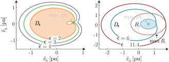
Figure 14: The neighborhood $B_{r}$, as an estimate of region of attraction within $D_{\epsilon}$, exists only if $\epsilon>3$ is chosen. The largest region of attraction is identified with $\epsilon=11.4$.

References

• [1] R. Musca, A. Vasile, and G. Zizzo, “Grid-forming converters. A critical review of pilot projects and demonstrators,” Renew. Sust. Energ. Rev., vol. 165, p. 112551, 2022.
• [2] R. Rosso, X. Wang, M. Liserre, X. Lu, and S. Engelken, “Grid-forming converters: Control approaches, grid-synchronization, and future trends—A review,” IEEE Open J. Ind. Appl., vol. 2, pp. 93–109, 2021.
• [3] F. Dörfler and D. Groß, “Control of low-inertia power systems,” Annu. Rev. Control Robot. Auton. Syst., vol. 6, pp. 415–445, 2023.
• [4] J. W. Simpson-Porco, F. Dörfler, and F. Bullo, “Synchronization and power sharing for droop-controlled inverters in islanded microgrids,” Automatica, vol. 49, no. 9, pp. 2603–2611, 2013.
• [5] F. Dörfler and F. Bullo, “Synchronization and transient stability in power networks and nonuniform Kuramoto oscillators,” SIAM J. Control Optim., vol. 50, no. 3, pp. 1616–1642, 2012.
• [6] N. Ainsworth and S. Grijalva, “A structure-preserving model and sufficient condition for frequency synchronization of lossless droop inverter-based AC networks,” IEEE Trans. Power Syst., vol. 28, no. 4, pp. 4310–4319, 2013.
• [7] J. Schiffer, R. Ortega, A. Astolfi, J. Raisch, and T. Sezi, “Conditions for stability of droop-controlled inverter-based microgrids,” Automatica, vol. 50, no. 10, pp. 2457–2469, 2014.
• [8] H. Wu and X. Wang, “Design-oriented transient stability analysis of grid-connected converters with power synchronization control,” IEEE Trans. Ind. Electron., vol. 66, no. 8, pp. 6473–6482, 2019.
• [9] L. Huang, H. Xin, Z. Wang, L. Zhang, K. Wu, and J. Hu, “Transient stability analysis and control design of droop-controlled voltage source converters considering current limitation,” IEEE Trans. Smart Grid, vol. 10, no. 1, pp. 578–591, 2019.
• [10] Z. Shuai, C. Shen, X. Liu, Z. Li, and Z. J. Shen, “Transient angle stability of virtual synchronous generators using Lyapunov’s direct method,” IEEE Trans. Smart Grid, vol. 10, no. 4, pp. 4648–4661, 2019.
• [11] J. Schiffer, D. Efimov, and R. Ortega, “Global synchronization analysis of droop-controlled microgrids—a multivariable cell structure approach,” Automatica, vol. 109, p. 108550, 2019.
• [12] M. Choopani, S. H. Hosseinian, and B. Vahidi, “New transient stability and LVRT improvement of multi-VSG grids using the frequency of the center of inertia,” IEEE Trans. Power Syst., vol. 35, no. 1, pp. 527–538, 2020.
• [13] E. Rokrok, T. Qoria, A. Bruyere, B. Francois, and X. Guillaud, “Transient stability assessment and enhancement of grid-forming converters embedding current reference saturation as current limiting strategy,” IEEE Trans. Power Syst., vol. 37, no. 2, pp. 1519–1531, 2022.
• [14] W. Du, Z. Chen, K. P. Schneider, R. H. Lasseter, S. Pushpak Nandanoori, F. K. Tuffner, and S. Kundu, “A comparative study of two widely used grid-forming droop controls on microgrid small-signal stability,” IEEE J. Emerg. Sel. Top. Power Electron., vol. 8, no. 2, pp. 963–975, 2020.
• [15] D. Pan, X. Wang, F. Liu, and R. Shi, “Transient stability of voltage-source converters with grid-forming control: A design-oriented study,” IEEE J. Emerg. Sel. Top. Power Electron., vol. 8, no. 2, pp. 1019–1033, 2020.
• [16] M. Colombino, D. Groß, J.-S. Brouillon, and F. Dörfler, “Global phase and magnitude synchronization of coupled oscillators with application to the control of grid-forming power inverters,” IEEE Trans. Autom. Control, vol. 64, no. 11, pp. 4496–4511, 2019.
• [17] D. Groß, M. Colombino, J.-S. Brouillon, and F. Dörfler, “The effect of transmission-line dynamics on grid-forming dispatchable virtual oscillator control,” IEEE Trans. Control Netw. Syst., vol. 6, no. 3, pp. 1148–1160, 2019.
• [18] I. Subotić, D. Groß, M. Colombino, and F. Dörfler, “A Lyapunov framework for nested dynamical systems on multiple time scales with application to converter-based power systems,” IEEE Trans. Autom. Control, vol. 66, no. 12, pp. 5909–5924, 2021.
• [19] X. He, V. Häberle, I. Subotić, and F. Dörfler, “Nonlinear stability of complex droop control in converter-based power systems,” IEEE Control Syst. Lett., vol. 7, pp. 1327–1332, 2023.
• [20] H. Yu, M. A. Awal, H. Tu, I. Husain, and S. Lukic, “Comparative transient stability assessment of droop and dispatchable virtual oscillator controlled grid-connected inverters,” IEEE Trans. Power Electron., vol. 36, no. 2, pp. 2119–2130, 2021.
• [21] M. A. Awal and I. Husain, “Transient stability assessment for current-constrained and current-unconstrained fault ride through in virtual oscillator-controlled converters,” IEEE J. Emerg. Sel. Top. Power Electron., vol. 9, no. 6, pp. 6935–6946, 2021.
• [22] C. Arghir and F. Dörfler, “The electronic realization of synchronous machines: Model matching, angle tracking, and energy shaping techniques,” IEEE Trans. Power Electron., vol. 35, no. 4, pp. 4398–4410, 2020.
• [23] A. Tayyebi, A. Anta, and F. Dörfler, “Grid-forming hybrid angle control and almost global stability of the DC–AC power converter,” IEEE Trans. Autom. Control, vol. 68, no. 7, pp. 3842–3857, 2023.
• [24] I. Subotić and D. Groß, “Power-balancing dual-port grid-forming power converter control for renewable integration and hybrid AC/DC power systems,” IEEE Trans. Control Netw. Syst., vol. 9, no. 4, pp. 1949–1961, 2022.
• [25] X. He, V. Häberle, and F. Dörfler, “Complex-frequency synchronization of converter-based power systems,” 2022, submitted to IEEE Trans. Control Netw. Syst. [Online]. Available: https://arxiv.org/abs/2208.13860
• [26] F. Milano, “Complex frequency,” IEEE Trans. Power Syst., vol. 37, no. 2, pp. 1230–1240, 2022.
• [27] G.-S. Seo, M. Colombino, I. Subotic, B. Johnson, D. Groß, and F. Dörfler, “Dispatchable virtual oscillator control for decentralized inverter-dominated power systems: Analysis and experiments,” in Proc. IEEE Appl. Power Electron. Conf. Expo., 2019, pp. 561–566.
• [28] M. Lu, “Virtual oscillator grid-forming inverters: State of the art, modeling, and stability,” IEEE Trans. Power Electron., vol. 37, no. 10, pp. 11 579–11 591, 2022.
• [29] L. Huang, H. Xin, and F. Dörfler, “$\mathcal{H}_{\infty}$-control of grid-connected converters: Design, objectives and decentralized stability certificates,” IEEE Trans. Smart Grid, vol. 11, no. 5, pp. 3805–3816, 2020.
• [30] S. P. Nandanoori, S. Kundu, W. Du, F. K. Tuffner, and K. P. Schneider, “Distributed small-signal stability conditions for inverter-based unbalanced microgrids,” IEEE Trans. Power Syst., vol. 35, no. 5, pp. 3981–3990, 2020.
• [31] K. Dey and A. M. Kulkarni, “Passivity-based decentralized criteria for small-signal stability of power systems with converter-interfaced generation,” IEEE Trans. Power Syst., vol. 38, no. 3, pp. 2820–2833, 2023.
• [32] J. C. Vasquez, J. M. Guerrero, A. Luna, P. Rodriguez, and R. Teodorescu, “Adaptive droop control applied to voltage-source inverters operating in grid-connected and islanded modes,” IEEE Trans. Ind. Electron., vol. 56, no. 10, pp. 4088–4096, 2009.
• [33] M. A. Awal and I. Husain, “Unified virtual oscillator control for grid-forming and grid-following converters,” IEEE J. Emerg. Sel. Top. Power Electron., vol. 9, no. 4, pp. 4573–4586, 2021.
• [34] B. Fan, T. Liu, F. Zhao, H. Wu, and X. Wang, “A review of current-limiting control of grid-forming inverters under symmetrical disturbances,” IEEE Open J. Power Electron., vol. 3, pp. 955–969, 2022.
• [35] M. A. Desai, X. He, L. Huang, and F. Dörfler, “Saturation-informed current-limiting control for grid-forming converters,” 2023, submitted to Electr. Power Syst. Res. and patent pending.
• [36] H. K. Khalil, Nonlinear Systems, 3rd ed.   Englewood Cliffs, NJ, USA: Prentice-Hall, 2002.
• [37] X. He and F. Dörfler, “Passivity and decentralized stability conditions for grid-forming converters,” 2023, submitted to IEEE Power Engineering Letters. [Online]. Available: https://arxiv.org/pdf/2310.09935.pdf
• [38] P. Vorobev, P.-H. Huang, M. Al Hosani, J. L. Kirtley, and K. Turitsyn, “High-fidelity model order reduction for microgrids stability assessment,” IEEE Trans. Power Syst., vol. 33, no. 1, pp. 874–887, 2018.
• [39] X. He, H. Geng, R. Li, and B. C. Pal, “Transient stability analysis and enhancement of renewable energy conversion system during LVRT,” IEEE Trans. Sustain. Energy, vol. 11, no. 3, pp. 1612–1623, 2020.
• [40] E. Panteley, A. Loria, and A. El Ati, “On the stability and robustness of stuart-landau oscillators,” IFAC-PapersOnLine, vol. 48, no. 11, pp. 645–650, 2015.
• [41] R. K. Miller and A. N. Michel, Ordinary differential equations, 1st ed.   New York, USA: Academic Press, 1982. [Online]. Available: https://doi.org/10.1016/C2013-0-11183-X