BONES: Near-Optimal Neural-Enhanced Video Streaming

Abstract.

Accessing high-quality video content can be challenging due to insufficient and unstable network bandwidth. Recent advances in neural enhancement have shown promising results in improving the quality of degraded videos through deep learning. Neural-Enhanced Streaming (NES) incorporates this new approach into video streaming, allowing users to download low-quality video segments and then enhance them to obtain high-quality content without violating the playback of the video stream. We introduce BONES, an NES control algorithm that jointly manages the network and computational resources to maximize the quality of experience (QoE) of the user. BONES formulates NES as a Lyapunov optimization problem and solves it in an online manner with near-optimal performance, making it the first NES algorithm to provide a theoretical performance guarantee. Our comprehensive experimental results indicate that BONES increases QoE by 4% to 13% over state-of-the-art algorithms, demonstrating its potential to enhance the video streaming experience for users. Our code and data will be released to the public.

1. Introduction

Video content dominates the Internet, accounting for more than 65% of its traffic volume (Sandvine, 2023). However, accessing high-quality video content is often hindered by insufficient and unstable network bandwidth between the video server and video player (i.e., client). This challenge of high-quality video streaming is even more significant when delivering higher-resolution or immersive videos, such as 4K/8K videos, 360-degree videos, and volumetric videos.

The traditional approach to maximizing the user’s quality of experience (QoE) is to use an adaptive bitrate (ABR) algorithm. An ABR algorithm typically runs within the video player and ensures that the video plays back continuously (i.e., without rebuffering) at the highest possible quality (i.e., bitrate). To achieve that goal, the ABR algorithm downloads lower-quality video segments when the available network bandwidth is low to prevent rebuffering and downloads higher-quality segments when the bandwidth is high. There has been extensive research on developing ABR algorithms for decades, with many known algorithms such as BOLA, Dynamic, Festive, MPC, Pensieve, etc (Spiteri et al., 2020, 2019; Huang et al., 2014; Jiang et al., 2012; Yin et al., 2015; Mao et al., 2017).

Neural-Enhanced Streaming (NES). Traditional video streaming relies on transmitting videos from the server to the client in the highest possible quality while ensuring continuous playback (Chakareski and Chou, 2006; Thomos et al., 2011; Chakareski et al., 2005). However, recent advances in machine learning open up a new possibility of transmitting videos from the server to the client in low quality, but neurally enhancing the video quality via deep-learning techniques at the client. Some examples of such neural enhancement include super-resolution (Lim et al., 2017; Liang et al., 2021), frame interpolation(Yue and Shi, 2023; Shi et al., 2022a), video inpainting (Suvorov et al., 2022; Zeng et al., 2020), video denoising (Claus and van Gemert, 2019; Tassano et al., 2020), point cloud upsampling (Yu et al., 2018; Li et al., 2019), and point cloud completion (Huang et al., 2020). NES methods incorporate this new approach into video streaming, allowing a tradeoff between communication resources for transmitting high-quality videos and computational resources for neural enhancement. Unlike ABR algorithms that only decide the quality of the video segment to download, an NES control algorithm decides on both the download quality and the enhancement option for each video segment.

Prior work on NES. While not as extensively studied as ABR algorithms, recent work on NES algorithms use reinforcement learning (RL) (Yeo et al., 2018; Zhang et al., 2020; Chen et al., 2020; Shi et al., 2022b; Zhang et al., 2021) or use a heuristic approach (Zhou et al., 2023; Zhang et al., 2022). However, prior NES algorithms do not have theoretical guarantees of their performance. Further, prior work only considers one enhancement option during inference, usually the one bringing the highest quality gain in real-time. This restricts the possible design space of enhancement options and disregards the broader benefits of utilizing diverse enhancements over a longer time horizon. Finally, existing NES methods are complex to deploy and slower to converge to the desired solution. Specifically, RL-based methods require a large training dataset and high training cost, but may still not adapt to real-world scenarios (Yan et al., [n. d.]). Other prior approaches that rely on model predictive control (MPC) compute a large decision table or heuristically solve an NP-hard problem, leading to an intractable solution (Yin et al., 2015; Zhou et al., 2023).

Our NES algorithm. To rectify the above shortcomings, we propose Buffer-Occupancy-based Neural-Enhanced Streaming (BONES), a client-side NES algorithm for on-demand video streaming. Specifically, BONES downloads video segments from a video provider’s server to a client device and then enhances these segments opportunistically using local computational resources. To ensure efficient scheduling of the available bandwidth and computational resources, BONES operates within a novel parallel-buffer system model and solves a Lyapunov optimization problem online. It has a provable near-optimal performance and exploits all available enhancement methods during inference, resulting in superior performance. Besides, BONES has a simple control algorithm with linear complexity, making it easy to deploy in production systems.

Our Contributions. We make the following contributions in our work.

1. Joint optimization of download and enhancement decisions. BONES generalizes the Lyapunov optimization approach of the ABR algorithm BOLA (Spiteri et al., 2020, 2019) to the NES problem of scheduling both bandwidth and computational resources. Our proposed parallel-buffer system model and online control algorithm allow for optimizing download and enhancement decisions jointly while conducting actual operations asynchronously, which largely contributes to the performance.

2. Theoretical guarantees and simple algorithm design. BONES is the first NES algorithm with a provable guarantee of its performance. Specifically, BONES achieves QoE that is provably within an additive factor of the offline optimal. Besides performance, BONES has the advantages of linear time complexity and simplicity in deployment.

3. Superior experimental performance with low overhead. Using extensive experiments under six enhancement settings and four network trace datasets, we demonstrate that BONES increases QoE by a range of values between 3.56% and 13.20% when compared with existing ABR and NES methods. In comparison to the default ABR algorithm of dash.js video player (Stockhammer, 2011), BONES can improve its QoE by $7.33\%$, which is equivalent to increasing the average visual quality by 5.22 in the VMAF score. Additionally, BONES offers a tradeoff between QoE improvements and resource overheads. BONES provides a modest increase in QoE with no overhead, but can provide full benefits with a modest overhead of no more than a 2.2 MB extra download.

2. Problem Formulation

Modern video streaming works by partitioning the video into segments, where each segment plays for a fixed amount of time (say, 4 seconds). The video player sequentially downloads each segment from a video server and renders the segment on the viewer’s device. To reduce the chances of rebuffering (i.e., freezing), each segment is downloaded and stored in a download buffer ahead of when it needs to be rendered. Each segment is encoded in multiple qualities. And an ABR algorithm chooses the quality to download in an online fashion with the goal of reducing rebuffering events and optimizing the QoE. As noted earlier, an NES algorithm also performs neural enhancements for downloaded segments prior to rendering. In this section, we first propose a system model for our NES system, capturing both the download and enhancement process in Sec. 2.1. Then, we formulate an optimization problem in Sec. 2.2 that is solved by our NES algorithm BONES. The main notations used in this paper are summarized in Tab. 1.

Table 1. Summary of main notations.

Notation	Description
$t_{k}$	the $k$-th time slot
$K_{n}$	index of the time slot where the $n$-th segment is downloaded
$T_{k}$	duration of time slot $t_{k}$
$d_{i}$	binary indicator to select the $i$-th download bitrate
$e_{j}$	binary indicator to select the $j$-th enhancement method
$Q^{d}(t_{k})$	download buffer level at time slot $t_{k}$
$Q^{e}(t_{k})$	enhancement buffer level at time slot $t_{k}$
$u^{d}(i,t_{k})$	download utility of the $i$-th bitrate in time slot $t_{k}$
$u^{e}(i,j,t_{k})$	enhancement utility of the $j$-th method for the $i$-th bitrate in time slot $t_{k}$
$\tilde{u}^{e}(i,j,t_{k})$	timely enhancement utility of the $j$-th method for the $i$-th bitrate in time slot $t_{k}$
$p$	duration of a video segment
$B_{i}(t_{k})$	the $i$-th download bitrate in time slot $t_{k}$
$S_{i}(t_{k})$	size of the video segment with the $i$-th bitrate in time slot $t_{k}$
$\omega(t_{k})$	average bandwidth in time slot $t_{k}$
$t^{e}(i,j)$	processing time to enhance a segment with the $i$-th bitrate using the $j$-th method
$T_{\text{end}}$	playback finishing time
$V$	parameter to control the trade-off between Lyapunov drift and penalty
$Q^{d}_{\max}$	maximum download buffer capacity
$u_{\max}$	maximum utility of a video segment
$T_{\min}$	minimum time slot duration
$T_{\max}$	maximum time slot duration
$u_{n}$	total utility of the $n$-th video segment
$\phi_{n}$	rebuffering time to download the $n$-th video segment
$\gamma$	hyper-parameter to control the trade-off between utility and smoothness
$\beta$	hyper-parameter to linearly control $V$

2.1. System Model

We show the system model of a traditional ABR algorithm in Fig. 1 and contrast it with the system model of BONES. Compared with a traditional ABR system that solely schedules bandwidth resources with one download buffer, our NES system incorporates an extra buffer and control flow to manage computational resources. In the BONES system model, the download buffer stores video segments that have been downloaded, and the enhancement buffer stores enhancement tasks waiting for computational resources. We first introduce the download process in the lower branch and then the enhancement process in the upper branch.

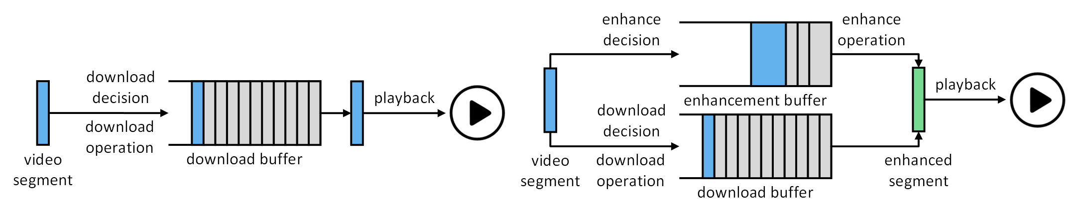
Figure 1. System model of traditional ABR algorithm (left) and BONES (right).

Suppose the video segment is indexed by $n\in[N]$, and the time slot is indexed by $k\in[K_{N}]$, where $K_{N}$ represents the index of the slot where the $N$-th (last) segment of the video content is downloaded. At the beginning of each time slot $t_{k}$, BONES makes both download and enhancement decisions for the next video segment.

The download decision determines whether to download the next segment in this time slot and at which bitrate to download it. Formally, we represent the possible choices for this decision variable using a vector $\mathbf{d}=(d_{1},\cdots,d_{I})$, where the indicator $d_{i}\in\{0,1\}$, $\sum_{i=1}^{I}d_{i}\leq 1$, and $I$ denotes the number of possible download bitrate options. In particular, $\sum_{i}d_{i}=0$ indicates no download, while $d_{i}=1$ indicates that the next segment will be downloaded at the $i$-th available bitrate $B_{i}(t_{k})$ at time slot $t_{k}$. A high download bitrate improves the video quality but consumes more network bandwidth, leading to a longer download time.

If the decision is to download, the segment will be retrieved at the desired bitrate and then added to the end of the download buffer, as illustrated in Fig. 1. The next time slot will commence immediately after the completion of the download. If there is no download in the present time slot, BONES waits for $\Delta$ milliseconds and starts the next slot. The video content is played back at a constant rate from the download buffer. However, if the download buffer is empty, the playback will freeze until new content is available, which results in rebuffering and negatively impacts the quality of experience (QoE) of the user.

Let length $p$ of the next video segment denote the temporal duration of its content in milliseconds. Assume that the $i$-th download option has been selected, i.e., ${d_{i}=1}$. Then, the segment’s size in bits can be expressed as ${S_{i}(t_{k})=B_{i}(t_{k})p}$. Next, let $\omega(t_{k})$ denote the average network bandwidth during $t_{k}$ in Kbps. We can then compute the duration of time slot $t_{k}$, i.e., the download time of the segment as $T_{k}=S_{i}(t_{k})/\omega(t_{k})$ milliseconds. Note that $T_{k}$ also captures the amount of downloaded content consumed by the client due to video playback during time slot $t_{k}$. Finally, let $Q^{d}(t_{k})$ denote the download buffer level, i.e., the total length of segments remaining in the buffer. We can formulate the download buffer dynamic as follows:

(1) $$Q^{d}(t_{k+1})=\max[Q^{d}(t_{k})-T_{k},0]+\sum_{i}d_{i}p.$$

At the start of $t_{k}$, we also decide whether to enhance the video segment and which enhancement method to apply. The enhancement decision is defined as a vector $\mathbf{e}=(e_{1},\cdots,e_{J})$, where the indicator $e_{j}\in\{0,1\}$. But slightly different from the download decision, we have $\sum_{j=1}^{J}e_{j}=1$, where $J$ denotes the number of possible enhancement methods. This is because we set the first enhancement method ($e_{1}$) as ”no enhancement” with zero finishing time and zero effect. $e_{j}=1$ indicates that the $j$-th available enhancement method will be applied to the video segment. An enhancement method using a larger deep-learning model typically offers greater quality improvement but takes more time to complete due to higher computational complexity.

A video segment will be pushed into the enhancement buffer at the moment it is pushed into the download buffer. When doing so, we are actually registering a new computation task to enhance this segment with the chosen enhancement method, and letting this task wait for resources in the enhancement buffer. Therefore, we define the length of a video segment in the enhancement buffer as the required time to finish its enhancement, denoted by $t^{e}(i,j)$. This computation time $t^{e}(i,j)$ is a function of the download option $i$ and the enhancement option $j$, as both the downloaded video quality and enhancement model can affect the computation speed. Here, we assume the computation time as a constant number pre-measured on the local device. Since the duration of a segment is usually different from the processing time of its enhancement task, a video segment often has different lengths in the two buffers, as illustrated in Fig. 1.

It is important to note that, though the enhancement decision is made before a segment enters the enhancement buffer, the actual computation takes place when the video segment leaves. This property enables BONES to optimize download and enhancement decisions jointly but perform the actual operations asynchronously in a non-blocking manner, which leads to superior performance. It also allows us to fit into a Lyapunov optimization framework (Neely, 2013) which can synchronously control multiple queues in a renewal process.

The departure of a segment from the enhancement buffer indicates the completion of its enhancement task. The enhancement buffer has the same departure rate as the download buffer, because in 1 second, we will playback 1-second video content and complete a 1-second computational task. Every video segment must go through both download and enhancement buffers to become an enhanced segment before playback. But the enhanced segment could be the same as the original if ”no enhancement” is selected. Let the enhancement buffer level $Q^{e}(t_{k})$ capture the aggregate length of computational tasks waiting in the buffer measured in milliseconds. Now, we can formulate the temporal evolution of the enhancement buffer as:

(2) $$Q^{e}(t_{k+1})=\max[Q^{e}(t_{k})-T_{k},0]+\sum_{ij}d_{i}e_{j}t^{e}(i,j).$$

2.2. Optimization Objective

There are three main goals in video streaming - improve video quality, reduce the rebuffering ratio, and avoid buffer overflow. Similarly to BOLA (Spiteri et al., 2020, 2019), we incorporate these three goals into a Lyapunov optimization problem. To improve the video quality, we aim to maximize a time-average utility function defined as

(3) $$\begin{split}\bar{u}&\triangleq\lim_{N\to\infty}\frac{\mathbb{E}\{\sum_{kij}d_{i}u^{d}(i,t_{k})+d_{i}e_{j}\tilde{u}^{e}(i,j,t_{k})\}}{\mathbb{E}\{T_{\text{end}}\}}\\ &=\frac{\lim_{K_{N}\to\infty}\frac{1}{K_{N}}\mathbb{E}\{\sum_{kij}d_{i}u^{d}(i,t_{k})+d_{i}e_{j}\tilde{u}^{e}(i,j,t_{k})\}}{\lim_{K_{N}\to\infty}\frac{1}{K_{N}}\mathbb{E}\{\sum_{k=1}^{K_{N}}T_{k}\}},\end{split}$$

where $u^{d}(i,t_{k})$ is the base utility of a video segment, $\tilde{u}^{e}(i,j,t_{k})$ is the extra utility obtained by neural enhancement, and $T_{\text{end}}$ is the playback finishing time. While the proposed algorithm works for any size of the video sequences, in our theoretical analysis, we further assume there are infinitely many video segments, i.e., $N\to\infty$. Because the gap between the total playback time and total download time is the time required to drain all the content out of the download buffer, we have $\mathbb{E}\{T_{\text{end}}\}-\mathbb{E}\{\sum_{k=1}^{K_{N}}T_{k}\}\leq Q^{d}_{\max}$, where $Q^{d}_{\max}$ is the maximum download buffer capacity. Since $Q^{d}_{\max}$ is finite, we further have $\lim_{K_{N}\to\infty}\mathbb{E}\{T_{\text{end}}\}=\lim_{K_{N}\to\infty}\mathbb{E}\{\sum_{k=1}^{K_{N}}T_{k}\}$. Based on this equation and the theory of renewal processes (Gallager, 2012), we can derive the last formula in Eq. 3. The final utility function is the expected sum of the download and enhancement utility in each time slot, averaged by the expected time slot duration.

Different from existing myopic NES methods that only consider the present time slot, we allow for selecting non-real-time enhancements and buffering of computation tasks over a longer time horizon. However, we must make sure that the enhancement of a segment is finished before its playback. Utilizing the property that the two buffers have the same departure rate, we know that an enhancement requiring $t^{e}(i,j)$ to finish will miss the playback deadline if $Q^{e}(t_{k})+\sum_{ij}d_{i}e_{j}t^{e}(i,j)>Q^{d}(t_{k})$. So we abandon such options by assigning them a negative infinity utility. The final enhancement utility function is expressed in Eq. 4, where $u^{e}(i,j)$ represents an enhancement method’s utility improvement pre-measured by the video provider and transmitted to the client via metadata. Specially, we have $t^{e}(i,1)=0,u^{e}(i,1,t_{k})=0,~{}\forall i,k$ for the ”no enhancement” option.

(4) $$\tilde{u}^{e}(i,j,t_{k})=\left\{\begin{aligned} &-\infty,~{}Q^{e}(t_{k})+\sum_{ij}d_{i}e_{j}t^{e}(i,j)>Q^{d}(t_{k}),\\ &u^{e}(i,j),\text{~{}otherwise}.\end{aligned}\right.$$

In order to reduce the rebuffering ratio, we aim to maximize the time-average playback smoothness function defined in Eq. 5. In particular, by maximizing the ratio of the total video length $\sum_{kij}d_{i}e_{j}p$ and the total playback time $T_{\text{end}}$, we are minimizing their difference, i.e., the total rebuffering time.

(5) $$\begin{split}\bar{s}&\triangleq\lim_{N\to\infty}\frac{\mathbb{E}\{\sum_{kij}d_{i}e_{j}p\}}{\mathbb{E}\{T_{\text{end}}\}}\\ &=\frac{\lim_{K_{N}\to\infty}\frac{1}{K_{N}}\mathbb{E}\{\sum_{kij}d_{i}e_{j}p\}}{\lim_{K_{N}\to\infty}\frac{1}{K_{N}}\mathbb{E}\{\sum_{k=1}^{K_{N}}T_{k}\}}.\end{split}$$

To prevent buffer overflow, we require both buffers to be rate stable, which is a relaxation of the strict buffer constraint. Rate stability ensures that the expected input rate is not greater than the expected output rate. We then establish the download buffer constraint as

(6) $$\lim_{K_{N}\to\infty}\frac{1}{K_{N}}\mathbb{E}\{\sum_{ki}d_{i}p\}\leq\lim_{K_{N}\to\infty}\frac{1}{K_{N}}\mathbb{E}\{\sum_{k}T_{k}\},$$

and the enhancement buffer constraint as

(7) $$\lim_{K_{N}\to\infty}\frac{1}{K_{N}}\mathbb{E}\{\sum_{k}d_{i}e_{j}t^{e}(i,j)\}\leq\lim_{K_{N}\to\infty}\frac{1}{K_{N}}\mathbb{E}\{\sum_{k}T_{k}\}.$$

Finally, we formulate the neural enhancement problem as

(8) $$\max_{\mathbf{d},\mathbf{e}}~{}~{}\bar{u}+\gamma\bar{s},\quad\text{s.t.,}\quad\text{Constraints}~{}\eqref{eq:rated},~{}\eqref{eq:ratee},$$

where the goal is to maximize the streaming session’s utility and smoothness under buffer constraints. The hyper-parameter $\gamma$ controls the trade-off between the smoothness and utility objectives. Note that our optimization target can be reduced to that of BOLA by setting $e_{1}=1$ (always choosing ”no enhancement”). This implies that our method can function as a neural enhancement streaming algorithm when enhancement is available or a conventional ABR algorithm, otherwise.

3. BONES: Control Algorithm and Theoretical Analysis

In this section, we first present our proposed control algorithm BONES in Sec. 3.1. Next, we visualize the decision plane of BONES and analyze the impact of system parameters in Sec. 3.2. At last, we rigorously prove the performance bound of BONES in Sec. 3.3.

3.1. Control Algorithm

Input: computation time matrix $T^{e}\in\mathbb{R}_{+}^{I\times J}$, total utility matrix $U\in\mathbb{R}^{N\times I\times J}$, segment size matrix $S\in\mathbb{R}_{+}^{N\times I}$ , maximum download buffer capacity $Q^{d}_{\max}$, maximum utility $u_{\max}$, segment duration $p$, hyper-parameters $\gamma$ and $\beta$

1 Initialize $O\in\mathbb{R}^{I\times J},\quad V=\beta\nicefrac{{((Q^{d}_{\max}-p)p)}}{{(u_{\max}+\gamma p)}}$

2 for $n\in[1,N]$ do

3       $t\leftarrow$ current timestamp

4       for $i\in[1,I]$ do

5             for $j\in[1,J]$ do

6                   $O[i,j]\leftarrow(Q^{d}(t)p+Q^{e}(t)T^{e}[i,j]-V(U[n,i,j]+\gamma p))/S[n,i]$

7                   if $Q^{e}(t)+T^{e}[i,j]>Q^{d}(t)$ then

8                         $O[i,j]\leftarrow-\infty$

9                        

10                   end if

11                  

12             end for

13            

14       end for

15      $i^{\prime},j^{\prime}\leftarrow\arg\min_{i,j}O$

16       download the $n$-th segment with the $i^{\prime}$-th bitrate, wait until the download finishes at $t^{\prime}$

17       if $Q^{e}(t^{\prime})+T^{e}[i^{\prime},j^{\prime}]>Q^{d}(t^{\prime})$ then

18             $j^{\prime}\leftarrow 0$

19            

20       end if

21      push the $n$-th segment into the enhancement buffer to enhance it with the $j^{\prime}$-th method

22       push the $n$-th segment into the download buffer

23       $\Delta t_{\text{sleep}}\leftarrow\max[Q^{d}(t^{\prime})+p-Q^{d}_{\max},0]$

24       wait for time $\Delta t_{\text{sleep}}$

25      

26 end for

Algorithm 1 BONES: A joint control algorithm for download and enhancement decisions

We develop an efficient online algorithm called BONES to compute the download and enhancement decisions. Solving problem (8) optimally in an online fashion is not practically feasible since the future values of the network bandwidth are uncertain. However, we show that BONES is within an additive factor of the offline optimal solution to the problem (8). Inspired by the Lyapunov optimization framework for renewal frames (Neely, 2013, 2010) and BOLA, BONES greedily minimizes the time-average drift-plus-penalty for each time slot. Specifically, the objective function involves the Lyapunov drift, defined as

(9) $$O_{D}(t_{k})=Q^{d}(t_{k})\sum_{i}d_{i}p+Q^{e}(t_{k})\sum_{ij}d_{i}e_{j}t^{e}(i,j),\\$$

and a penalty function defined as

(10) $$O_{P}(t_{k})=-(\sum_{ij}d_{i}u^{d}(i,t_{k})+d_{i}e_{j}\tilde{u}^{e}(i,j,t_{k})+\gamma d_{i}p).$$

We also need to divide our objective by the time slot duration $T_{k}=S_{i}(t_{k})/\omega(t_{k})$, but the random variable $\omega(t_{k})$ can be omitted in the optimization.

Altogether, the optimization problem that BONES aims to solve in each time slot is given below:

(11) $$\min_{\mathbf{d},\mathbf{e}} ~{}\frac{O_{D}(i,t_{k})+VO_{P}(i,j,t_{k})}{\sum_{i}d_{i}S_{i}(t_{k})}$$

s.t., $$~{}d_{i}\in\{0,1\}~{}\forall i,~{}\sum d_{i}\leq 1,$$

$$~{}e_{j}\in\{0,1\}~{}\forall j,~{}\sum e_{j}=1,$$

where $V$ is a trade-off factor between the Lyapunov drift and the penalty. Note that BONES relies solely on the download and enhancement buffer levels $Q^{d}(t_{k})$ and $Q^{e}(t_{k})$ in its operation without using any information about the available network bandwidth. Thus, BONES is named as a “buffer-occupancy-based” method.

We present the basic control algorithm of BONES in Algorithm 1. The algorithm receives a matrix of computation time $T^{e}\in\mathbb{R}_{+}^{I\times J}$ measured locally, a matrix of total utility $U\in\mathbb{R}^{N\times I\times J}$ from metadata, a matrix of segment size $S\in\mathbb{R}_{+}^{N\times I}$ from metadata, and some constant numbers and hyper-parameters as indicated in the input argument of Algorithm 1. The entries of the total utility matrix include the aggregate values of the download utility $u^{d}_{n}$ and the enhancement utility $u^{e}_{n}$ for each segment and enhancement option, i.e., $U[n,i,j]=u^{d}_{n}(i)+u^{e}_{n}(i,j)$. Note that BONES can also run with average utility and segment size if per-segment data is unavailable.

Concretely, the BONES algorithm operates as follows. The algorithm firstly computes $V$ according to Eq. 13 (Line 2 in Algorithm 1). Then for each video segment, BONES solves Eq. 11 by traversing all possible combinations of download and enhancement options and choosing the one with the minimum objective score (Lines 3 - 13). BONES downloads the video segment at the bitrate given by the solution and waits for the completion of the download. Once the segment is downloaded, BONES will check whether the previously-decided enhancement option is still applicable and pushes a computation task to the enhancement buffer only if it can be finished on time (Lines 15 - 18). BONES also pushes the video segment into the download buffer. At last, BONES will pause downloading until the download buffer can hold one more segment (Lines 20 - 21). Note that the stopping criterion here is implemented differently from the theory. This is because we can know exactly when BONES should stop downloading and how long it should sleep, by assigning $V$ a special upper bound. The impact of different values of $V$ on the performance of BONES will be discussed in Sec. 3.3.

BONES has a linear complexity of $O(IJ)$ in each iteration, where $I$ and $J$ are the numbers of possible choices for bitrate and enhancement options. Besides, the computation of objective scores can be fully parallelized. As a result, BONES runs efficiently in real-time and is easy to deploy. Based on the primary control algorithm here, we propose two additional heuristics in Sec. 5.3 to further improve the practical performance of BONES.

3.2. Decision Plane

To better understand our algorithm, we depict its 2D decision plane with respect to buffer levels under a hypothetical scenario involving two types of low-resolution (LR) segments and high-resolution (HR) segments. And there is only one type of enhancement method for LR segments. We present four variants of BONES decision planes in Fig. 2 under different parameter settings.

The decision plane of BONES. Starting from the lower left corner of a decision plane, the download buffer is empty and the viewer is in urgent need of content. In this case, BONES selects to quickly download LR segments without initiating enhancements. As the download buffer level increases, BONES still downloads LR segments but has time to enhance them and achieve higher visual quality. Once the download buffer level is high enough, BONES can pursue the highest quality by downloading HR segments since enhancement can never be perfect (enabling less quality than HR). When the download buffer is almost full, BONES suspends further downloading to prevent buffer overflow. According to Eq. 4, BONES will stop enhancing segments if the enhancement buffer level is close to the download buffer level, so it will never enter the upper left white triangle. If enhancements are unavailable on the device, the orange region vanishes and the control plane becomes a 1D function of the download buffer level, which implies BONES is reduced to BOLA. To conclude, this simple scenario demonstrates that BONES consistently exhibits reasonable behavior.

The impact of system parameters. Fig. 2 also illustrates the impact of system settings and hyper-parameter settings on the decisions of BONES. Compared with the “Basic” setting, we increase the computation speed by $2\times$ in “Faster Computation” as if BONES runs on more powerful computational hardware. In this case, the area of downloading and enhancing LR segments increases, meaning that neural enhancement becomes more desirable with more computational resources available.

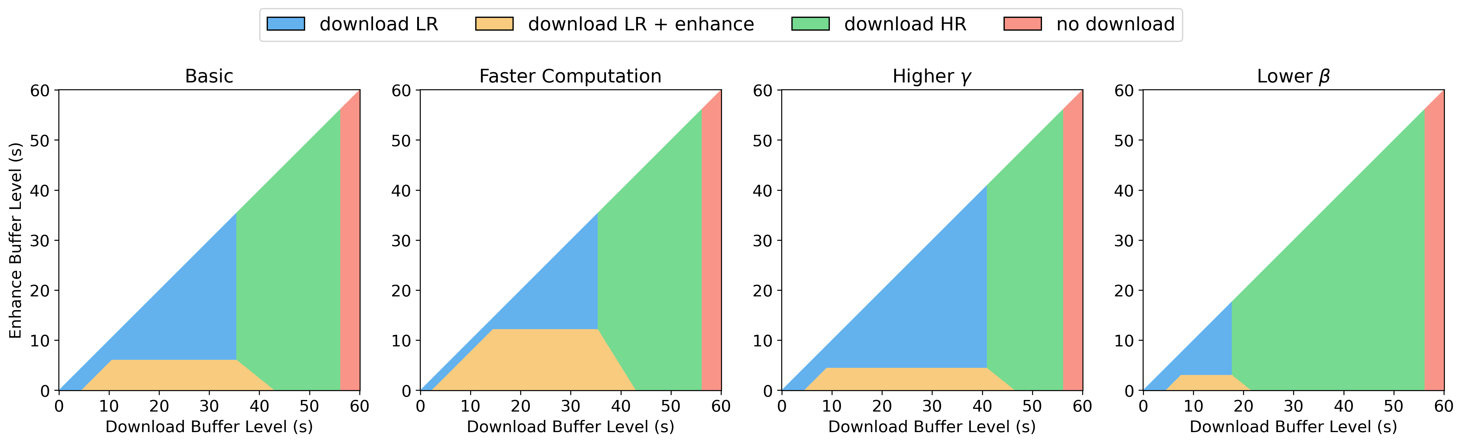
Figure 2. The decision plane of BONES. Parameter settings from left to right are as follows. “Basic”: $\gamma p=10,\beta=1$, $1\times$ computation speed. “Faster Computation”: $2\times$ computation speed. “Higher $\gamma$”: $\gamma p=50$. “Lower $\beta$”: $\beta=0.5$.

Recall that BONES has 2 hyper-parameters — $\gamma$ and $\beta$. Parameter $\gamma$ trades off between visual quality and playback smoothness (rebuffering ratio) in Eq. 8. In practice, we tune $\gamma$ together with the constant segment duration $p$. Parameter $\beta$ linearly controls $V$, the trade-off factor between Lyapunov drift and penalty in BONES optimization objective Eq. 11. In the “Higher $\gamma$” setting, we increase $\gamma p$ from 10 to 50, making BONES prefers a lower rebuffering ratio than higher visual quality. As a result, BONES increases the area of downloading LR segments and requests download bitrate in a more conservative manner. In the “Lower $\beta$” setting, we decrease $\beta$ from 1 to 0.5, suppressing the penalty term in the optimization objective Eq. 11. Due to the diminishing return effect of visual quality, each bit in an LR video segment provides more visual quality scores than that of an HR segment. Therefore, the penalty term in Eq. 11 prefers downloading LR segments and performing enhancements (see the structure of utility divided by segment size). On the opposite, the Lyapunov drift term prefers HR segments. This explains why BONES will download more HR segments as a consequence of lower $\beta$ and $V$ in this setting. We also provide empirical evidence of how BONES is affected by its hyper-parameters in Sec. 5.4.

3.3. Performance Bound

In this subsection, we rigorously analyze the performance of BONES and establish near-optimal guarantees. The analysis shares the same high-level logical flow with BOLA, but since BONES introduces the addition of an enhancement buffer, there are important differences in the details of the analysis. Theorem 1 bounds the size of the download buffer and shows that BONES does not violate the buffer capacity. Secondly, Theorem 2 bounds the performance of BONES with respect to that of the offline optimal solution.

Theorem 1.

Assume $Q^{d}(0)=0,Q^{e}(0)=0$, and $0<V\leq\frac{(Q^{d}_{\max}-p)p}{u_{\max}+\gamma p}$ , where $u_{\max}$ denotes the maximum utility. Then, the following holds: $Q^{d}(t_{k})\leq V\frac{u_{\max}+\gamma p}{p}+p$, and $Q^{d}(t_{k})\leq Q^{d}_{\max}$.

We present a proof in Appendix A. Theorem 1 shows that the download buffer level has a finite bound of $O(V)$ and will never exceed the maximum capacity. The intuition here is to design a special upper bound for $V$, which ensures BONES to select ”no download” if the download buffer level is higher than $Q^{d}_{\max}-p$. In this way, BONES will download only when the download buffer can accept one more segment. Since the enhancement buffer is a virtual queue without any storage space, its occupancy is not a concern.

In order to prove the performance bound of BONES, we first show that there exists an optimal stationary i.i.d. algorithm independent of the buffer occupancy for problem Eq. 8, achieving the objective $\bar{u}^{*}+\gamma\bar{s}^{*}$. Based on that, we can derive the following theorem.

Theorem 2.

Assume $t^{e}\leq t^{e}_{\max}$, $T_{\min}\leq T_{k}\leq T_{\max},~{}\forall k$, and $t^{e}_{\max},T_{\min},T_{\max}$ are finite. Then, we have:

(12) $$\bar{u}^{\prime}+\gamma\bar{s}^{\prime}\geq\bar{u}^{*}+\gamma\bar{s}^{*}-\frac{p^{2}+(t^{e}_{\max})^{2}+2T_{\min}T_{\max}}{2VT_{\min}},$$

where $\bar{u}^{\prime}+\gamma\bar{s}^{\prime}$ is the objective score of BONES.

Proofs for the existence of the offline optimal and Theorem 2 are given in Appendix B. While BONES can achieve an objective $\bar{u}^{\prime}+\gamma\bar{s}^{\prime}$ for Eq. 8, the optimal algorithm can achieve $\bar{u}^{*}+\gamma\bar{s}^{*}$. Theorem 2 shows that the performance gap of BONES toward this optimal algorithm is finitely bounded by $O(1/V)$. In other words, BONES can achieve near-optimal performance.

Results in the above theorems show that the performance of BONES depends on the value of parameter $V$. In the implementation of BONES, we use a hyper-parameter $\beta\in[0,1]$ to linearly control $V$ as follows.

(13) $$V=\beta\frac{(Q^{d}_{\max}-p)p}{u_{\max}+\gamma p}.$$

Putting together the results in Theorems 1 and 2, one can observe that BONES has a $O(V,1/V)$ trade-off between the download buffer level and the performance gap toward the optimal algorithm. It means one can increase $V$ to improve the performance of BONES. Empirical results in Sec. 5.4 verify this theoretical observation, showing that the QoE of BONES increases with $V$. However, increasing $V$ will increase the buffer level, thus increasing the time delay between downloading a segment and playing it back. Live streaming can be negatively affected by such behavior, but it may not be as much of an issue in on-demand video streaming. Besides, there is an upper cap for $V$ to prevent buffer overflow.

4. Experimental Evaluation

In this section, we introduce our experiment design. We first define the QoE metrics in Sec. 4.1, then present the implementation details in Sec. 4.2. We describe the neural enhancement methods used in our experiments in Sec. 4.3. Last, the comparison algorithms are listed in Sec. 4.4.

4.1. Performance Metric

To evaluate the overall performance of video streaming algorithms, we report the experimental results using a commonly-used notion of QoE that includes visual quality, quality oscillation, and rebuffering ratio. More formally, we have

(14) $$\text{QoE}=\frac{1}{N}\sum_{n=1}^{N}u_{n}-\alpha_{1}\frac{1}{N-1}\sum_{n=1}^{N-1}|u_{n+1}-u_{n}|-\alpha_{2}\frac{1}{N}\sum_{n=1}^{N}\phi_{n},$$

where $u_{n}$ is the total utility of a segment summing up the download utility $u^{d}_{n}$ and the enhancement utility $u^{e}_{n}$. And $\phi_{n}$ is the rebuffering time for each segment. The first term in Eq. 14 represents the average visual quality, the second term represents the average quality oscillation, and the third term is the average rebuffering time per segment. This notion of QoE is widely used in prior work, e.g., MPC-based methods (Yin et al., 2015; Zhou et al., 2023; Yan et al., [n. d.]; Nam et al., 2021) and RL-based methods (Mao et al., 2017; Yeo et al., 2018).

Although ABR-only algorithms typically assume utility (visual quality) as a function of bitrate, it is not a suitable metric in NES systems. This is because bitrate only applies to compressed videos, not raw pixels after computational processing. Therefore, we choose the VMAF score (Aaron et al., 2015) as the visual quality metric in our experiments, which is closer to human vision than other objective metrics like PSNR or SSIM. VMAF score ranges from 0 to 100, the higher, the better. We assign the highest-resolution video segments with the maximum score of 100 and invalid enhancement options with negative infinity scores. We measure the rebuffering time in milliseconds. And we set the trade-off factors $\alpha_{1}=1,\alpha_{2}=0.1$ as in method (Zhou et al., 2023), meaning that 1 QoE score is equivalent to the average visual quality of 1 VMAF score, average quality oscillation of 1 VMAF score, or per-segment rebuffering time of 10 milliseconds ($0.25\%$ rebuffering ratio in our case).

4.2. Implementation Settings

We develop a unified simulation environment for both ABR and NES algorithms to efficiently examine their performance. Our simulator extends Sabre (Spiteri et al., 2019), which was used to evaluate BOLA with around $2\%$ error in bitrate, $5\%$ error in oscillation, and no error in rebuffering toward real video players. Our simulation environment and all its algorithms are implemented using Python. And all deep-learning methods are implemented by PyTorch. We use a 636-second 30-fps video “Big Buck Bunny” for streaming. The video is chunked into 4-second segments and encoded in 5 resolutions of 240p/360p/480p/720p/1080p with bitrate of 400/800/1200/2400/4800 Kbps.

Table 2. Details of network trace datasets.

Dataset	3G	4G	FCC-SD	FCC-HD
Mean Bandwidth (Kbps)	1184	31431	6081	17127
Standard Variance of Bandwidth (Kbps)	818	14058	11615	4018
Number of Traces	86	40	1000	1000

We test all algorithms over 4 network trace datasets used in Sabre, including 3G traces (Riiser et al., 2013), 4G traces (van der Hooft et al., 2016), and two subsets of FCC traces (Commission, 2016). Differently, we exclude those 3G traces with an average bandwidth lower than 400 Kbps, the lowest option on our bitrate ladder. We present numerical details of our testing datasets in Tab. 2.

4.3. Enhancement Settings

Table 3. Enhancement model details. From left to right: #layers, #channels, upscale factor, model size (KB).

Model	Quality	240p	360p	480p	720p
NAS-MDSR	low	20,9,4,43	20,8,3,36	20,4,2,12	6,2,1,2
	medium	20,21,4,203	20,18,3,157	20,9,2,37	6,7,1,5
	high	20,32,4,461	20,9,3,395	20,18,2,128	6,16,1,17
	ultra	20,48,4,1026	20,42,3,819	20,26,2,259	6,26,1,41
IMDN	low	3,6,4,34	3,6,3,29	3,6,2,26	-
	medium	5,12,4,111	5,12,3,103	5,12,2,96	-
	high	6,32,4,760	6,32,3,736	6,32,2,719	-
	ultra	6,64,4,2824	6,64,3,2777	6,64,2,2743	-

We utilize 5 enhancement settings (6 if “no enhancement” is counted) to demonstrate that BONES can manage any enhancement method with any amount of computational power.

We first adopt the pervasively-used enhancement method NAS-MDSR (Yeo et al., 2018, 2020; Dasari et al., 2020), a content-aware Super-Resolution (SR) model that can overfit one individual video and upscale any resolution to 1080p. We further assume that the client-side computational hardware is an Nvidia GTX 1080ti GPU card. Under this setting, there are 5 enhancement quality levels (no enhancement, low, medium, high, and ultra) for each of the 4 low-resolution download options (240p, 360p, 480p, and 720p). More details about the deep-learning model can be found in Tab. 3. Besides, the visual quality and computation speed of each enhancement option are illustrated in Fig. 3, where zero computation speed implies the enhancement is not applicable. Generally, as the download bitrate and the enhancement quality level increase, the visual quality will increase and the computation speed will decrease. This trend also holds for other enhancement settings we introduce below.

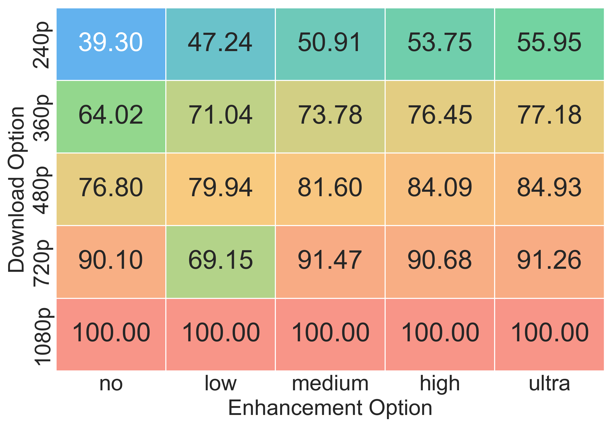
(a) Visual quality (VMAF).

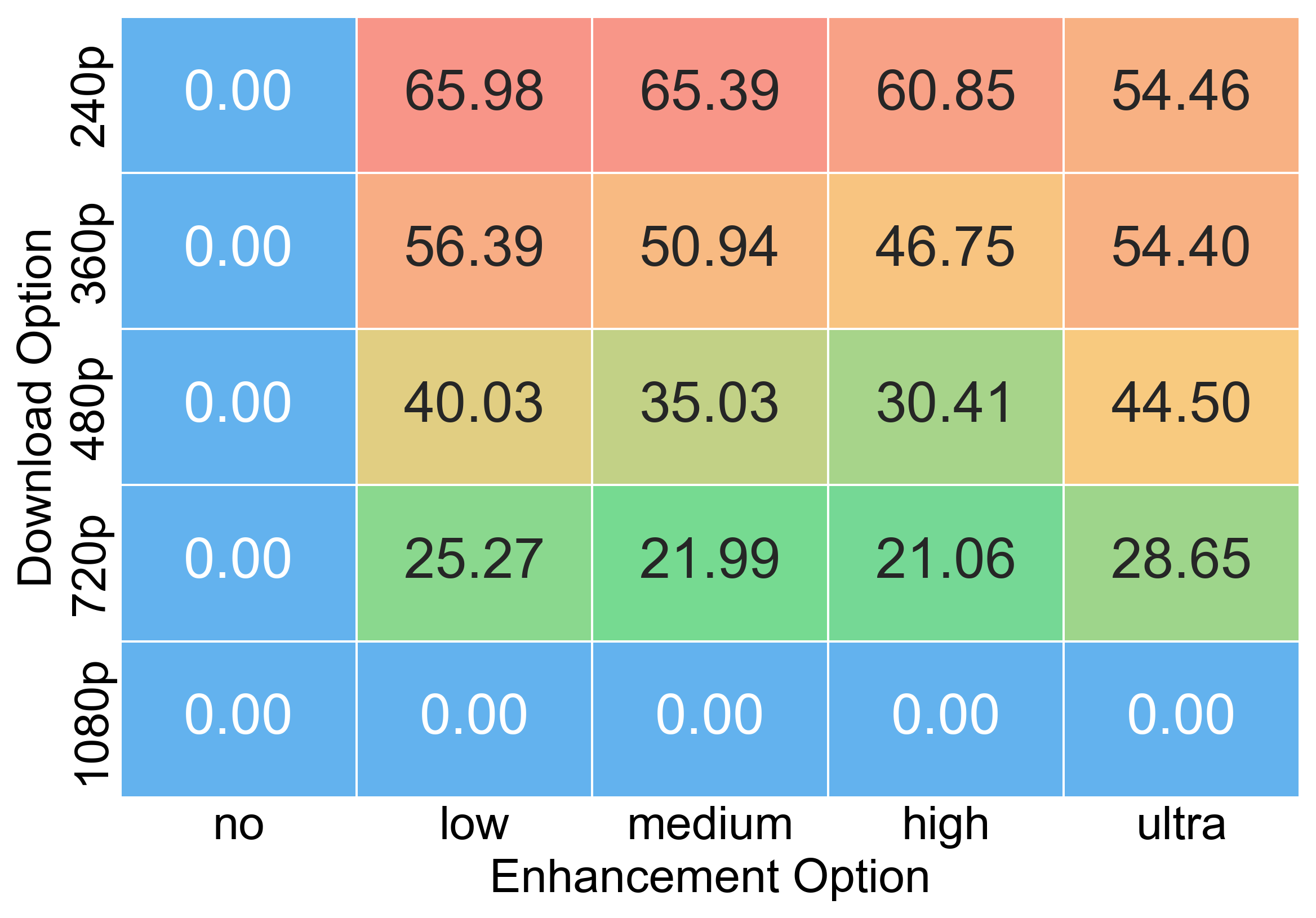
(b) Computation speed (fps).

Figure 3. Enhancement performance under NAS-MDSR setting.

Beyond NAS-MDSR, we adopt IMDN (Hui et al., 2019) as another SR enhancement method. We offer 4 quality levels for 240p, 360p, and 480p videos to upsample them to 1080p. The low and medium quality levels are based on the IMDN-RTC structure, while the high and ultra levels are based on the vanilla IMDN. Model details of IMDN can also be found in Tab. 3. As for the training technique, we explore both content-agnostic IMDN and content-aware IMDN. A content-agnostic IMDN is trained over a generic video dataset DIV2K (Agustsson and Timofte, 2017). Such a generic model can enhance any video but brings less quality improvement. In comparison, content-aware IMDN is trained over our target video to overfit its content. This strategy offers better enhancement performance but introduces overhead in training cost and startup latency. A more detailed discussion exists in Sec. 5.5. The computational hardware for IMDN is either GTX 2080ti or GTX 3060ti GPU card. Altogether, we create 4 enhancement settings for IMDN by traversing all combinations of training techniques and computational hardware.

4.4. Comparison Algorithms

We compare BONES with the following ABR-only algorithms.

1. BOLA (Spiteri et al., 2020) makes download decisions by solving a Lyapunov optimization problem only related to the buffer level.

2. Dynamic (Spiteri et al., 2019) switches between BOLA and a throughput-based algorithm based on carefully-designed heuristic rules.

3. FastMPC (Yin et al., 2015) formulates bitrate adaptation as an MPC optimization problem and makes download decisions according to a pre-computed solution table.

4. Buffer-based method (Huang et al., 2014) chooses bitrate using a piecewise linear function of buffer level.

5. Throughput-based method (Jiang et al., 2012) chooses the maximum bitrate under the estimated network bandwidth.

6. Pensieve (Mao et al., 2017) uses deep RL to make download decisions. We train the RL agent on 10,000 randomly selected FCC traces (Commission, 2016) using the Asynchronous Advantage Actor-Critic (A3C) algorithm with identical training settings as in the original paper.

We further augment ABR-only algorithms with a greedy enhancement strategy, denoted by the symbol $*$ on the right of algorithm names. Specifically, we let the ABR algorithms make download decisions while simultaneously choosing the enhancement option that brings the most utility improvement in real-time. To avoid interrupting playback, enhancements will only be applied if it can be finished on time. This greedy enhancement strategy is simple and will not affect the download performance of ABR algorithms. However, it only leads to sub-optimal performance because the download decision maker and the enhancement decision maker share no knowledge with each other. Beyond ABR algorithms, we also compare BONES with the following NES algorithms.

1. NAS (Yeo et al., 2018) controls both download and enhancement processes using an RL agent. The NAS RL agent is designed and trained similarly to Pensieve’s, with the additional consideration of a greedy real-time enhancement strategy. We did not reproduce the scalable model download approach in NAS, which can be viewed as providing more enhancement options.

2. PreSR (Zhou et al., 2023) solves an MPC problem online with the heuristic to pre-fetch and enhance only “complex” segments of the video.

5. Experimental Results

In this section, we first report the comprehensive comparison results in Sec. 5.1. Second, we further analyze the performance under restricted network conditions in Sec. 5.2. Then, we propose and examine additional heuristics that improve the practical performance of BONES in Sec. 5.3. We report the impact of hyper-parameters on the performance in Sec. 5.4. Finally, we analyze the overhead of neural enhancement in Sec. 5.5.

5.1. Overall Performance

Table 4. Overall performance comparison under different enhancement settings. Evaluated metrics include visual quality (VMAF), quality oscillation (VMAF), rebuffering rate (%), and composite QoE. * denotes the ABR method is augmented with greedy enhancement. The optimal results are marked in bold.

Method	Qual.	Osc.	Rebuf.	QoE	Method	Qual.	Osc.	Rebuf.	QoE
No Enhancement					NAS-MDSR, Content-Aware, GTX 1080ti
BOLA	82.90	4.05	2.21	69.98	BOLA *	85.45	3.66	2.21	72.93
Dynamic	84.62	3.73	2.43	71.14	Dynamic*	86.62	3.43	2.43	73.44
FastMPC	87.90	3.33	4.22	67.65	FastMPC*	89.70	3.22	4.22	69.56
Buffer	85.27	4.10	2.93	69.44	Buffer*	87.47	3.66	2.93	72.07
Throughput	80.10	3.59	1.93	68.77	Throughput*	83.43	3.33	1.93	72.36
Pensieve	89.23	4.01	4.17	68.50	Pensieve*	91.16	3.47	4.17	70.96
NAS	-	-	-	-	NAS	89.20	4.40	2.92	73.08
PreSR	-	-	-	-	PreSR	89.24	4.17	4.65	66.45
BONES	-	-	-	-	BONES	89.23	3.07	2.52	76.05
IMDN, Content-Agnostic, GTX 2080ti					IMDN, Content-Aware, GTX 2080ti
BOLA *	83.99	3.92	2.21	71.20	BOLA *	84.84	3.76	2.21	72.22
Dynamic*	85.62	3.63	2.43	72.25	Dynamic*	86.11	3.49	2.43	72.87
FastMPC*	88.46	3.27	4.22	68.26	FastMPC*	88.88	3.33	4.22	68.63
Buffer*	86.09	3.97	2.93	70.39	Buffer*	86.83	3.78	2.93	71.32
Throughput	81.76	3.45	1.93	70.57	Throughput*	82.59	3.35	1.93	71.50
Pensieve*	89.90	3.79	4.17	69.39	Pensieve*	90.19	3.71	4.17	69.76
NAS	88.18	4.66	2.92	71.81	NAS	88.35	4.57	2.92	72.06
PreSR	88.65	4.39	4.57	65.95	PreSR	88.79	4.20	4.51	66.53
BONES	88.40	3.52	2.80	73.64	BONES	88.97	3.47	2.55	75.29
IMDN, Content-Agnostic, GTX 3060ti					IMDN, Content-Aware, GTX 3060ti
BOLA *	84.85	3.77	2.21	72.21	BOLA *	84.75	3.83	2.21	72.05
Dynamic*	86.39	3.49	2.43	73.14	Dynamic*	86.49	3.42	2.43	73.32
FastMPC*	89.12	3.15	4.22	69.06	FastMPC*	89.17	3.21	4.22	69.03
Buffer*	86.91	3.80	2.93	71.38	Buffer*	86.77	3.85	2.93	71.19
Throughput*	82.58	3.36	1.93	71.48	Throughput*	83.46	3.34	1.93	72.38
Pensieve*	90.50	3.60	4.17	70.18	Pensieve*	91.05	3.50	4.17	70.83
NAS	88.98	4.39	2.92	72.88	NAS	89.17	4.38	2.92	73.08
PreSR	89.18	4.11	4.63	66.53	PreSR	88.85	4.20	4.52	66.55
BONES	88.49	3.37	2.64	74.52	BONES	89.38	3.12	2.47	76.36

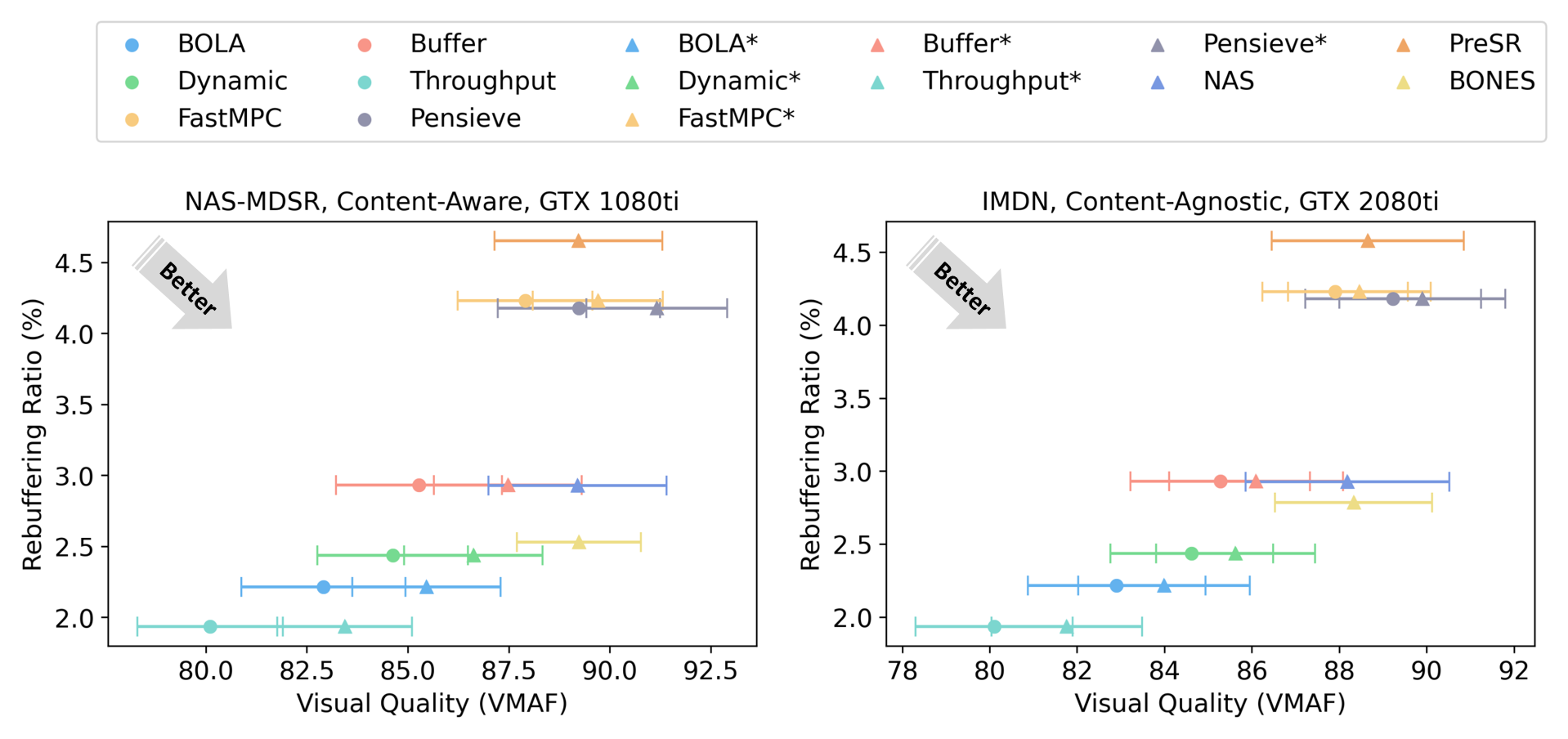
Figure 4. Performance comparison under two enhancement settings. The error bar represents the average visual quality oscillation. Higher quality, lower oscillation, and lower rebuffering ratio are better. * denotes the ABR method is augmented with a greedy enhancement strategy.

We present the performance of BONES and other benchmark methods averaged across all network trace datasets in Tab. 4 and Fig. 4. In Tab. 4, we report the QoE score defined in Eq. 14 as well as its three components (visual quality, quality oscillation, rebuffering ratio). The results are grouped under six settings, one setting without enhancement and five with different enhancement settings, one with NAS-MDSR, and four with IMDN as discussed in Sec. 4.3. We also provide visual representations of the three QoE components for each method under two enhancement settings in Fig. 4. Among ABR-only algorithms, we find that Dynamic, the default ABR algorithm of dash.js video player  (Stockhammer, 2011), reaches the best balance between the three metrics and achieves the highest QoE. Yet BONES can still improve its QoE by at most $7.33\%$, which is equivalent to increasing the average visual quality by 5.22 VMAF scores or decreasing the rebuffering ratio by $1.30\%$.

By augmenting ABR-only algorithms with the greedy enhancement strategy, their QoE benefits from the additional usage of computational resources. The greedy enhancement strategy will not affect the download behavior of an ABR algorithm, thus keeping its rebuffering ratio unchanged. But by upgrading the low-quality downloaded segments, neural enhancement increases the visual quality and reduces quality oscillation, leading to an average of $2.81\%$ QoE improvement across all kinds of augmentations. However, this enhancement strategy is decoupled from the download decision and thus leads to sub-optimal performance. In contrast, BONES makes joint decisions and outperforms all the augmented ABR algorithms.

As for NES methods, we find that both NAS and PreSR perform well under high-bandwidth scenarios but poorly if the network condition is weak. In Sec. 5.2, we further scrutinize the robustness of different algorithms under different network trace datasets. Our experimental results suggest that it’s hard for NAS to adapt to data distribution far from the training set. Similarly, (Yan et al., [n. d.]) reports that RL-based methods have limited generalization ability and may not adapt to heavy-tailed real-world network traces. In comparison, BONES is a control-theoretic algorithm that does not require any learning process, making it easy and robust to deploy under versatile scenarios.

We note that the unsatisfactory performance issue of PreSR comes from its reliance on sub-optimal heuristics. PreSR formulates an NP-hard MPC optimization problem and solves it online with heuristics. However, these heuristics only explore limited solutions and may miss better solutions in the decision space. As a result, PreSR can perform even worse than its backbone method FastMPC. In contrast, our method BONES covers the entire decision space of its backbone BOLA and only brings benefit, which is theoretically shown in Sec. 3.1 and empirically verified here.

By studying the four variants of IMDN enhancement settings, we find that the content-aware model performs better than the content-agnostic one as it overfits the content of a specific video. Nevertheless, content-aware enhancement requires costly training toward an individual video and increases the startup latency due to model downloading before video streaming. We postpone the detailed overhead analysis to Sec. 5.5. Besides, we find that the performance of neural enhancement increases with better computational hardware (GTX 3060ti than GTX 2080ti), which is intuitive since more computational resources enable more powerful enhancements.

In conclusion, our method BONES consistently outperforms existing ABR and NES methods by $3.56\%\sim 13.20\%$ in QoE averaged across all network conditions and all enhancement settings.

5.2. Sensitivity to Network Condition

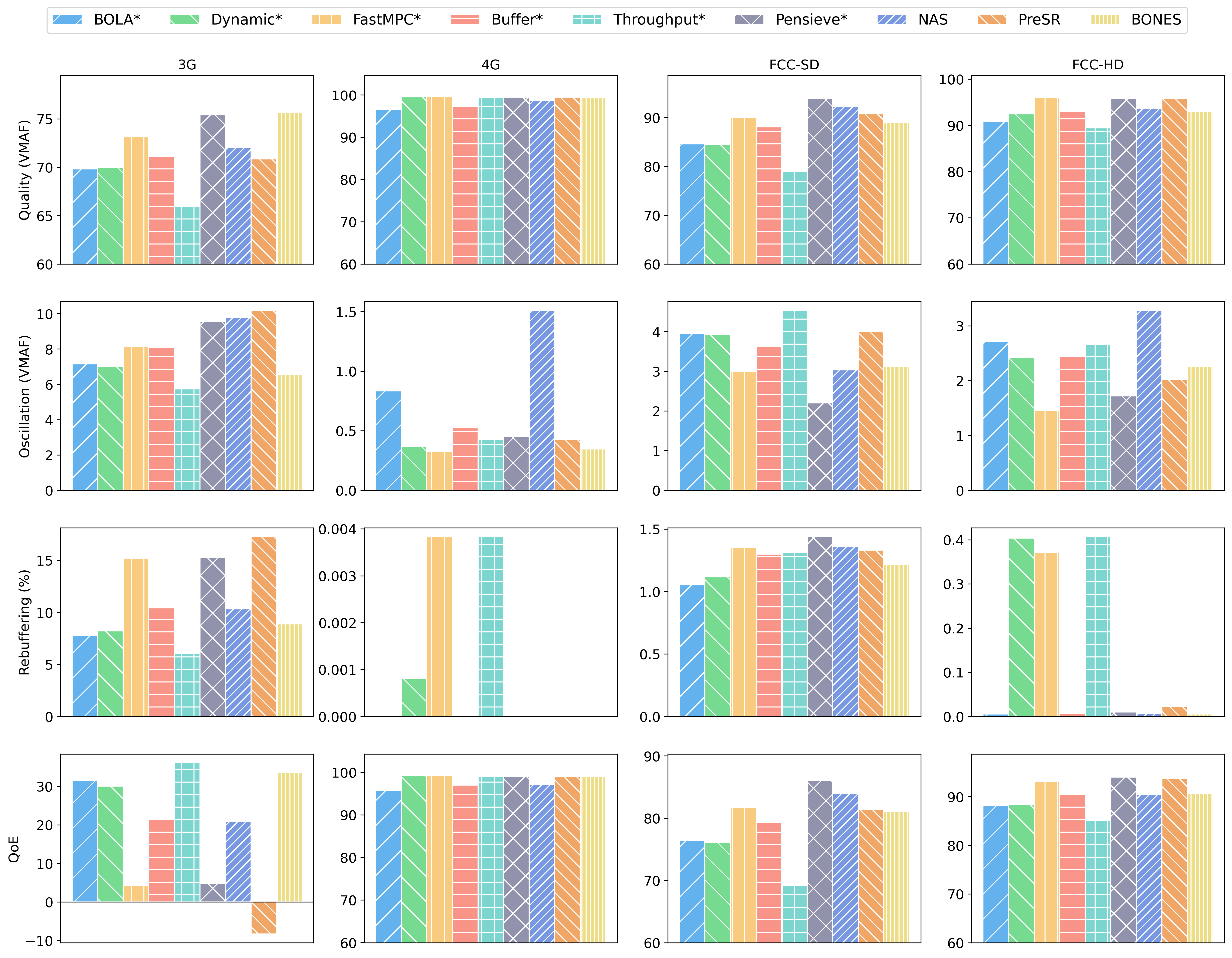
Figure 5. Performance comparison on different network trace datasets under NAS-MDSR enhancement.

To investigate the sensitivity of different algorithms to the network conditions, we further break down the results under the NAS-MDSR enhancement setting in Tab. 4 across four different network traces and report them in Fig. 5. Based on the results, we find that the performance of video streaming algorithms varies drastically with network conditions. For example, the throughput-based algorithm outperforms others on the low-bandwidth 3G dataset due to its conservative request of bitrate. However, this behavior does not generalize well to high-bandwidth conditions. Especially the throughput-based method performs worst on the FCC-SD dataset because the high variance of bandwidth leads to a misprediction of throughput. On the other hand, FastMPC, Pensieve, and PreSR perform well under good network conditions via aggressive bitrate requests. But they incur severe rebuffering events on 3G datasets. Unlike other methods, BONES behaves robustly across all network conditions, maintaining a stable QoE even under challenging low-bandwidth scenarios.

5.3. Practical Improvement

In this subsection, we introduce two additional heuristics to further advance the performance of BONES and report their empirical improvement.

Download Process Monitoring. Since the network bandwidth can vary abruptly in practice, a decision may become out-of-date when the corresponding video segment is under download. For example, downloading a high-quality segment may incur rebuffering if the bandwidth drops in midway. In such a case, it is wise to abort the current download and select a lower-quality segment. We implement this in a similar way to BOLA, allowing our algorithm to monitor the bandwidth variations during download processes and regret its previous decision if necessary. During the download process of a segment, BONES periodically recomputes the current decision’s objective score via a modified version of Eq. 11, where $S_{i}(t_{k})$ is replaced with the remaining size to download. BONES also computes the objective scores of other options. If a better option is found, BONES will abandon the ongoing download and switch to the new solution.

Automatic Hyper-Parameter Tuning. We observe that the hyper-parameter setting of BONES is sensitive to the network condition. Under poor network conditions, it is advisable to adopt a conservative strategy with lower quality and a lower rebuffering ratio, while under good conditions, an aggressive strategy is preferred. Inspired by Oboe (Akhtar et al., 2018), we develop an automatic hyper-parameter tuning mechanism for BONES in accordance with different network conditions. In the offline phase, we generate synthetic network traces with different average bandwidths (25 levels from 200 to 5000 Kbps), different bandwidth variances (10 levels from 500 to 5000 Kbps), and different latency (2 levels from 20 to 100 ms). Then we search for the optimal hyper-parameter $\beta$ (10 levels from 0.1 to 1) and $\gamma p$ (10 levels from $10$ to $100$) under each network condition that maximizes the QoE. During the online deployment phase, BONES estimates the network condition using the exponentially weighted moving average before each decision interval. BONES then adjusts its hyper-parameters to the offline optimal accordingly.

Empirical Results. We conduct an ablation study for practical improvement techniques and present the results under the NAS-MDSR enhancement setting in Tab. 5. Note that those versions without automatic hyper-parameter tuning are assigned with the optimal hyper-parameters found by grid search ($\beta=1$, $\gamma p=10$). As experimental results imply, Download Process Monitoring can reduce the rebuffering ratio by regretting previous decisions during bandwidth valley. While Automatic Hyper-Parameter Tuning can contribute to the performance of BONES mostly in visual quality. When both techniques are applied, BONES could achieve the maximum QoE improvement of $1.48\%$. In summary, this ablation study verifies the effectiveness of our practical improvement techniques.

Table 5. Ablation study for practical improvements.

Method	Quality (VMAF)	Oscillation (VMAF)	Rebuffering (%)	QoE
Basic	88.64	3.17	2.62	74.95
Monitoring	88.76	3.03	2.52	75.62
Auto-Tuning	89.22	3.16	2.58	75.71
Both	89.23	3.07	2.52	76.05

5.4. Sensitivity to Hyper-Parameter

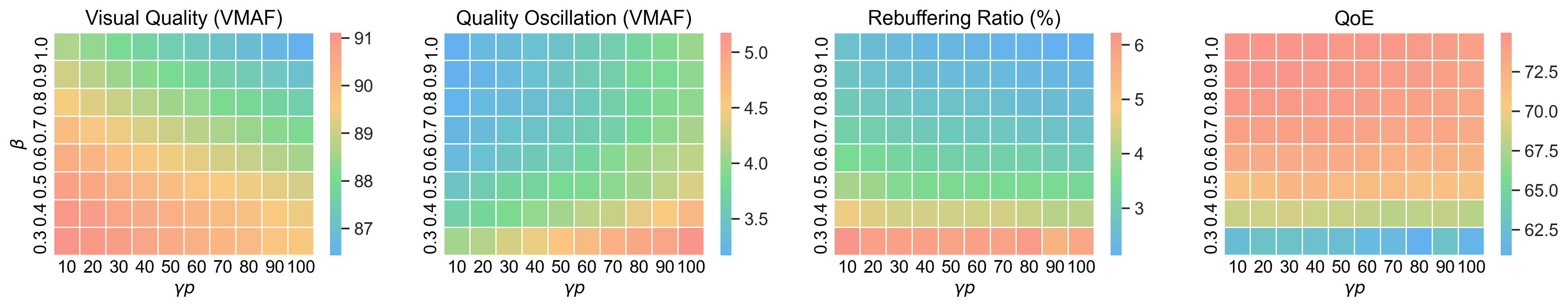
Figure 6. Performance of BONES with respect to hyper-parameter settings.

In this section, we comprehensively investigate the impact of hyper-parameters on the performance of BONES. It is worth noting that, in practice, one may leverage the Automatic Hyper-Parameter Tuning scheme in Sec. 5.3 instead of manually adjusting parameters. From the experimental results under NAS-MDSR enhancement settings in Fig. 6, we find that increasing $\gamma$ generally leads to lower visual quality, higher quality oscillation, and a lower rebuffering ratio. As explained in Sec. 3.2, a higher $\gamma$ makes BONES download more low-bitrate segments, trading quality for playback smoothness. Besides, due to the diminishing return of visual quality, low-bitrate segments span wider in quality scores. Thus downloading more low-quality segments brings more oscillations. We also find that a higher $\beta$ leads to lower visual quality, lower quality oscillation, and a lower rebuffering ratio. From our theoretical analysis in Sec. 3.2 we know that, by increasing the weight on the penalty term of optimization objective Eq. 11, BONES downloads more low-bitrate segments and performs more enhancements, resulting in lower quality and fewer rebuffering events. Additionally, since neural enhancement can improve visual quality and reduce the visual quality disparities between segments, increasing $\beta$ also alleviates quality oscillations. Lastly, empirical results verify that higher $\beta$ (so does $V$) positively contributes to the QoE. This conclusion roughly aligns with the observation in Theorem 2, despite the QoE here being defined in a slightly different way than the optimization objective.

5.5. Overhead Analysis

While neural enhancement significantly improves the QoE of video streaming, it incurs additional overhead in two aspects - training cost and startup latency. In this section, we analyze the overhead for both content-agnostic and content-aware neural enhancement models.

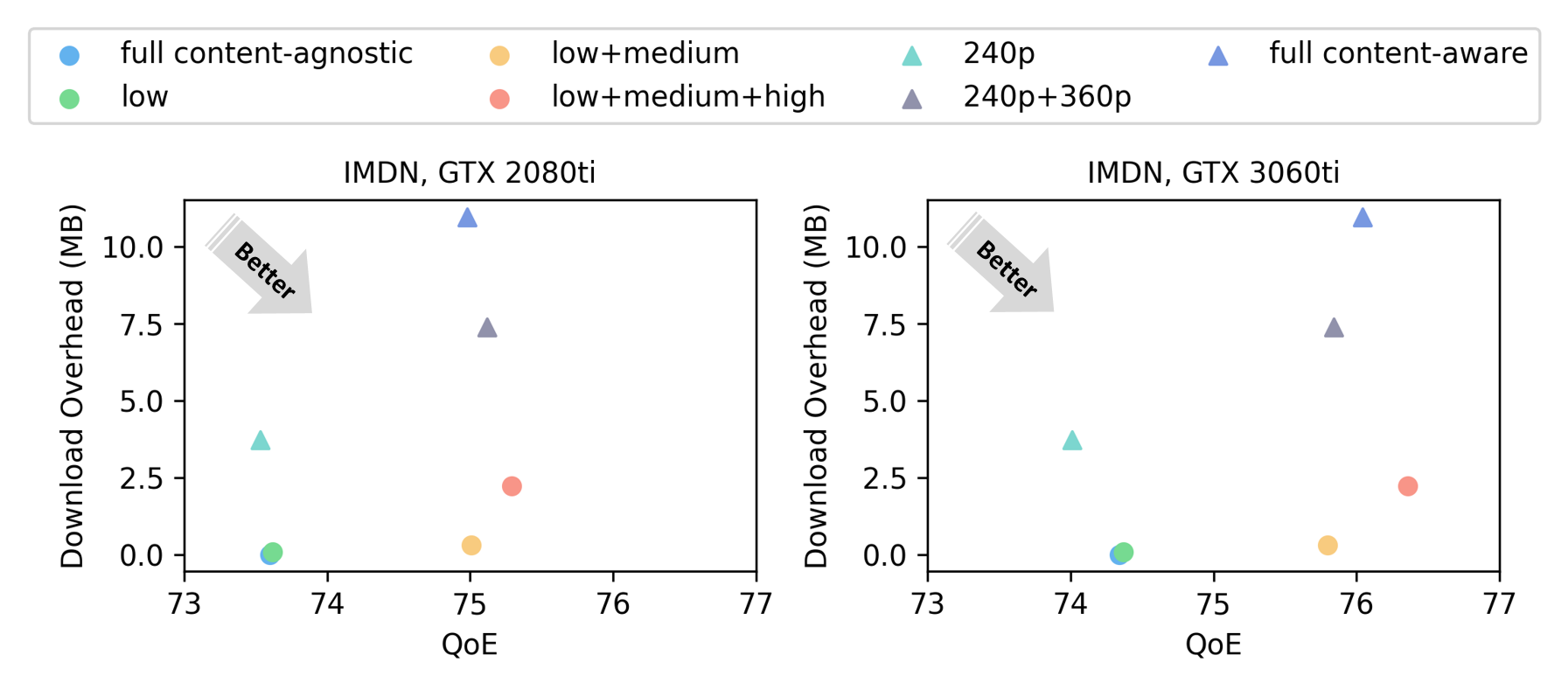
Figure 7. Performance of BONES with respect to download overhead.

A content-agnostic model is trained over a general video dataset. It is downloaded once and used to enhance all videos, so it only incurs a one-time training cost and will not impact the startup latency. However, content-agnostic methods can only provide limited QoE improvement as shown in Sec. 5.1. A content-aware model performs better since it is trained over a specific video, or more efficiently, fine-tuned toward a specific video from the content-agnostic backbone. NAS (Yeo et al., 2018) reports that a typical fine-tuning will take 10 minutes for each video, and the benefit of enhancement will cover this additional training cost after streaming the video for 30 hours. So as a rule of thumb, one may apply content-aware enhancements only for popular videos while using the content-agnostic counterpart for others.

Content-aware enhancements also increase the startup latency of video playback, because a corresponding model must be downloaded before streaming a video. Unlike other methods, BONES allow choosing different enhancement methods from a pool of enhancement methods on the fly. This behavior leads to more QoE improvement but requires pre-downloading more models, which may further deteriorate the startup latency. Therefore, we study the trade-off between performance and download overhead in Fig. 7, using IMDN as an example. Specifically, we plot QoE of BONES using content-agnostic IMDN and the additional download overhead (0 MB here) in Fig. 7. We do the same for a full content-aware IMDN, which requires downloading 4 quality levels $\times$ 3 bitrate levels $=12$ models. And then we start to remove some models from the enhancement method pool. For example, low means that we only keep the low-quality model, and 240p means that we only keep enhancement methods for the 240p bitrate. From the results, we find that low-quality content-aware models themselves can provide slightly more QoE than content-agnostic models with a download overhead of 89 KB. And we can gain almost all the benefits by downloading the first two quality levels with only 310 KB. Surprisingly, we can even outperform the full model by downloading the first three quality levels using 2215 KB. It means that the ultra-level IMDN model is actually a trap for BONES, dragging its performance by occupying enormous resources but providing marginal improvements. This result shows that the selection of the enhancement method pool could be critical for BONES performance, and we leave this for future research.

In summary, BONES only one-time training costs or costs that can be covered in the short run. Additionally, BONES can offer lower QoE with zero overhead, or full benefits with a startup download of no more than 2.2 MB. These findings indicate that BONES greatly boosts QoE with low to moderate costs.

6. Related Work

Adaptive Bitrate Streaming. The ABR algorithm selects the download bitrate for video segments in adaptation to the varying network bandwidth. ABR algorithms can be generally classified into three categories. First, buffer-based methods adapt the bitrate purely based on the client’s buffer level. For example, the method in (Huang et al., 2014) chooses the bitrate according to a piecewise linear function of the buffer level. BOLA (Spiteri et al., 2020) makes download decisions by solving a Lyapunov optimization problem with respect to the buffer level. Our method could be viewed as an extension of BOLA from ABR to the new NES scenario. Second, throughput-based methods utilize the prediction of future network bandwidth. FESTIVE (Jiang et al., 2012) estimates bandwidth using harmonic mean and chooses the maximum bitrate under that estimation. Fugu (Yan et al., [n. d.]) proposes a more accurate download time prediction module based on fully-connected neural networks, while Xatu (Yan et al., [n. d.]) employs a long short-term memory (LSTM) network for prediction. Third, mixed-input algorithms consider both buffer level and estimated throughput inputs. Pensieve (Mao et al., 2017) takes these states as input and trains a reinforcement-learning (RL) agent. FastMPC (Yin et al., 2015) formulates bitrate adaptation as an online control problem and solves it via model predictive control (MPC). Dynamic (Spiteri et al., 2019) switches between a throughput-based method and BOLA to take advantage of both.

Neural Enhancement. Neural enhancement refers to any method that improves video quality via deep learning. It typically encompasses the following areas. Super-resolution (SR) aims at improving the resolution of images (Lim et al., 2017; Hui et al., 2019; Liang et al., 2021) and videos (Chan et al., 2021, 2022). To reduce the training and inference cost of SR models, Li et al. (Li et al., 2022) overfit the first video segment and then fine-tune the model toward the following segments. Wang et al. (Wang et al., 2022) introduce heuristics like training with smaller patches and decreasing the update frequency. DeepStream (Amirpour et al., 2022) further introduces scene grouping, frame sub-sampling, and model compression. Frame interpolation aims at improving the frame rate of videos (Yue and Shi, 2023; Shi et al., 2022a). Inpainting methods can complete the missing region of images (Suvorov et al., 2022) or videos (Zeng et al., 2020). Denoising methods effectively reduce noise in videos (Claus and van Gemert, 2019; Tassano et al., 2020). Apart from 2D videos, point cloud upsampling (Yu et al., 2018; Li et al., 2019) increases the density of 3D point cloud objects in volumetric videos, and point cloud completion (Huang et al., 2020) makes them whole. In this paper, we used NAS-MDSR (Yeo et al., 2018) and IMDN (Hui et al., 2019) SR models as our enhancement methods, but our control algorithm BONES can be integrated with any subset of the above algorithms.

Neural-Enhanced Streaming. NES incorporates neural enhancement methods into video streaming algorithms and enables high-quality content delivery by leveraging both bandwidth and computational resources. NAS (Yeo et al., 2018) is the first method to integrate SR models into on-demand video streaming. It develops a content-aware SR model called NAS-MDSR and utilizes a Pensieve-like RL agent to manage both download and enhancement processes. SRAVS (Zhang et al., 2020) adopts RL controllers and a lightweight SR model while proposing a double-buffer system model. PreSR (Zhou et al., 2023) pre-fetches and enhances “complex” segments that bring the most quality improvement and bandwidth reduction. It formulates the problem as MPC and solves it heuristically. Our method is most similar to these approaches.

Neural enhancement can be applied beyond the scope of client-side on-demand video streaming. LiveNAS (Kim et al., 2020) upsamples low-resolution videos at the ingest server for live streaming. NEMO (Yeo et al., 2020) increases the computational efficiency of SR by only enhancing selected ”anchor” frames. Based on LiveNAS and NEMO, NeuroScaler (Yeo et al., 2022) can enhance live streams at scale. Dejavu (Hu et al., 2019) improves the quality of the current frame in live video conferencing using historical knowledge. And VISCA (Zhang et al., 2021) deploys SR models on edge-based cache servers. Beyond the regular 2D videos, recent work applied NES to 360-degree and volumetric videos. The substantial bandwidth requirement of these videos makes the assistance of neural enhancement even more appealing. SR360 (Chen et al., 2020) uses RL to make viewport prediction and enhancement decisions for delivering 360 videos. Sophon (Shi et al., 2022b) pre-fetches and enhances semantically salient tiles in a 360 video. Madarasingha et al. (Madarasingha and Thilakarathna, 2022) enhance 360 videos with both SR and frame interpolation at edge servers. YuZu (Zhang et al., 2022) streams volumetric videos and enhances them using point cloud upsampling. Emerging studies of virtual reality streaming systems also pursue optimal policies for joint allocation of the available computational and communication resources(Chakareski et al., 2023; Gupta et al., 2023; Chakareski et al., 2022), where the concept of enhancement is not limited to deep-learning methods.

While the above methods are based on RL or heuristic optimization, we formulate and near-optimally solve a Lyapunov optimization problem. Our method BONES is the first NES algorithm with a theoretical performance bound. Furthermore, BONES has been proven to exhibit exceptional performance through numerous experiments, while also possessing the benefits of being simple and robust in deployment.

7. Conclusion

This paper proposed BONES, an NES algorithm incorporating neural enhancement into video streaming, allowing users to download low-quality video segments and then enhance them via deep-learning models. Residing in a parallel-buffer system model, BONES jointly optimizes download and enhancement decisions to maximize the QoE by solving a Lyapunov optimization problem. BONES achieves the performance within an additive factor toward offline optimal, making it the first NES algorithm with a theoretical performance guarantee. We thoroughly investigate the influencing factors of BONES, which align well with the empirical results. Extensive experiments verify that BONES can outperform existing ABR and NES methods by $3.56\%\sim 13.20\%$ in QoE, and maintain stable performance under challenging network conditions. Besides, BONES offers a trade-off between performance and overhead, which will download at most 2.2 MB of additional data. We release our source code and data to the public, expecting BONES to become a new baseline for the NES problem.

There are some limitations to the current work, which open future research directions. Firstly, we assume the computation time of enhancement is static or can be accurately predicted. This may not hold in reality, especially when the algorithm is competing with other applications for computational resources. Secondly, we only consider scheduling one type of enhancement (super-resolution) using one additional enhancement buffer. In practice, it is possible to simultaneously apply multiple enhancements, which may require the scheduling of multiple enhancement buffers. Thirdly, we only consider a client-side on-demand video streaming scenario. Deploying a streaming algorithm at the cloud servers, edge servers, or for live streaming may raise other interesting challenges. Given the simplicity of algorithm design, bounded theoretical performance, and superior empirical performance of BONES, in future work, we will explore the possibility of generalizing BONES or other Lyapunov-based algorithms to more-dynamic, multi-buffer, multi-point, and low-latency systems.

Appendix A Proof of Theorem 1

Proof.

We prove the inequality $Q^{d}(t_{k})\leq V\frac{u_{\max}+\gamma p}{p}+p$ by induction. The bound holds for $k=1$ as $Q^{d}(t_{1})=Q^{d}(0)=0$. Suppose it also holds for some $k$. Then there are two cases for $k+1$.

(1) $Q^{d}(t_{k})\leq V\frac{u_{\max}+\gamma p}{p}$. From Eq. 1 we know $Q^{d}(t_{k})$ can increase by at most $p$ in one single time slot. Hence, we have $Q^{d}(t_{k+1})\leq V\frac{u_{\max}+\gamma p}{p}+p$.

(2) $V\frac{u_{\max}+\gamma p}{p}<Q^{d}(t_{k})\leq V\frac{u_{\max}+\gamma p}{p}+p$. In this case, we have

$$V<\frac{Q^{d}(t_{k})p}{u_{\max}+\gamma p}\leq\frac{Q^{d}(t_{k})p+Q^{e}(t_{k})t^{e}(i,j)}{u^{d}(i,t_{k})+\tilde{u}^{e}(i,j,t_{k})+\gamma p},~{}\forall i,j.$$

This makes $O_{D}(t_{k})+VO_{P}(t_{k})>0,~{}\forall\mathbf{d},\mathbf{e},$ in Eq. 11 and forces the control algorithm not to download. As a result, $Q^{d}(t_{k+1})<Q^{d}(t_{k})$.

Till now, we have proven $Q^{d}(t_{k})\leq V\frac{u_{\max}+\gamma p}{p}+p$. Combining it with $V\leq\frac{(Q^{d}_{\max}-p)p}{u_{\max}+\gamma p}$ from assumption, we have $Q_{d}(t_{k})\leq Q^{d}_{\max}$ and the proof is complete. ∎

Appendix B Proof of Theorem 2

Lemma 0.

Denote the optimal objective of problem Eq. (8) as $\bar{u}^{opt}+\gamma\bar{s}^{opt}$. There exists a stationary i.i.d. algorithm for this problem that has the following properties for any $\delta>0$.

1. $\bar{u}^{*}+\gamma\bar{s}^{*}\leq\bar{u}^{opt}+\gamma\bar{s}^{opt}+\delta.$

2. $\frac{\mathbb{E}\{\sum_{ki}d^{*}_{i}p\}}{\mathbb{E}\{\sum_{k}T^{*}_{k}\}}\leq 1+\delta.$

3. $\frac{\mathbb{E}\{\sum_{kij}d^{*}_{i}e^{*}_{j}t^{e}(i,j)\}}{\mathbb{E}\{\sum_{k}T^{*}_{k}\}}\leq 1+\delta.$

Proof.

Problem Eq. (8) is formulated as maximizing time-averaged objective under time-averaged constraints in a system with variable-size renewal frames. This lemma can be directly derived from Lemma 1 in (Neely, 2013). ∎

Based on Lemma 1, we prove Theorem 2 as follows.

Proof.

In the following proof, we will use superscript ^′ to denote the decisions of BONES, and $*$ for those of the optimal i.i.d. algorithm.

Following the framework of Lyapunov optimization over renewable frames (Neely, 2013), we define the Lyapunov function $L(t_{k})$ as

(15) $$L(t_{k})\triangleq\frac{1}{2}(Q^{d}(t_{k})^{2}+Q^{e}(t_{k})^{2}).$$

Define $\mathbf{Q}(t_{k})=[Q^{d}(t_{k}),Q^{e}(t_{k})]$, then the conditional Lyapunov drift is formulated as

(16) $$D(t_{k})\triangleq\mathbb{E}\{L(t_{k+1})-L(t_{k})|\mathbf{Q}(t_{k})\}.$$

The drift $D(t_{k})$ is bounded by

(17) $$\begin{split}D(t_{k})&\leq\frac{1}{2}p^{2}+\frac{1}{2}(t^{e}_{\max})^{2}+T_{\max}\mathbb{E}\{T_{k}|\mathbf{Q}(t_{k})\}\\ &+Q^{d}(t_{k})\mathbb{E}\{\sum_{i}d_{i}p-T_{k}|\mathbf{Q}(t_{k})\}\\ &+Q^{e}(t_{k})\mathbb{E}\{\sum_{ij}d_{i}e_{j}t^{e}(i,j)-T_{k}|\mathbf{Q}(t_{k})\}.\end{split}$$

For the sake of simplicity, we denote $\frac{1}{2}p^{2}+\frac{1}{2}(t^{e}_{\max})^{2}$ as $C$. Now we reuse $O_{D}(t_{k})$ in Eq. 9 and $O_{P}(t_{k})$ in Eq. 10. Adding $V$ times $E\{O_{P}(t_{k})|\mathbf{Q}(t_{k})\}$ on both sides and simplifying the formula using $E\{O_{D}(t_{k})|\mathbf{Q}(t_{k})\}$, we have

(18) $$\begin{split}&D(t_{k})+V\mathbb{E}\{O_{P}(t_{k})|\mathbf{Q}(t_{k})\}\\ &\leq C+(T_{\max}-Q^{d}(t_{k})-Q^{e}(t_{k}))\mathbb{E}\{T_{k}|\mathbf{Q}(t_{k})\}\\ &+\mathbb{E}\{O_{D}(t_{k})+VO_{P}(t_{k})|\mathbf{Q}(t_{k})\}.\end{split}$$

Recall that the time slot duration can be computed by $T_{k}=(\sum_{i}d_{i}S_{i})/\omega(t_{k})$. As our algorithm greedily minimizes the objective defined in Eq. 11, we can derive

(19) $$\begin{split}&\frac{O_{D}^{\prime}(t_{k})+VO_{P}^{\prime}(t_{k})}{\sum_{i}d^{\prime}_{i}S_{i}}\leq\frac{O_{D}^{*}(t_{k})+VO_{P}^{*}(t_{k})}{\sum_{i}d_{i}^{*}S_{i}}\\ \Rightarrow&\frac{O_{D}^{\prime}(t_{k})+VO_{P}^{\prime}(t_{k})}{(\sum_{i}d_{i}^{\prime}S_{i})/\omega(t_{k})}\leq\frac{O_{D}^{*}(t_{k})+VO_{P}^{*}(t_{k})}{(\sum_{i}d_{i}^{*}S_{i})/\omega(t_{k})}\\ \Rightarrow&\mathbb{E}\{O_{D}^{\prime}(t_{k})+VO_{P}^{\prime}(t_{k})|\mathbf{Q}(t_{k})\}\\ &\leq\frac{\mathbb{E}\{T_{k}^{\prime}|\mathbf{Q}(t_{k})\}}{\mathbb{E}\{T_{k}^{*}|\mathbf{Q}(t_{k})\}}\mathbb{E}\{O_{D}^{*}(t_{k})+VO_{P}^{*}(t_{k})|\mathbf{Q}(t_{k})\}.\end{split}$$

We then apply Eq. 19 to Eq. 18 and bring in the definition of Eq. 3, Eq. 5. Since the total video length or total enhancement time is less or equal to the total playback time, we have

(20) $$\begin{split}&D^{\prime}(t_{k})+V\mathbb{E}\{O_{P}^{\prime}(t_{k})|\mathbf{Q}(t_{k})\}\\ &\leq C+T_{\max}\mathbb{E}\{T_{k}^{\prime}|\mathbf{Q}(t_{k})\}-V(\bar{u}^{*}+\gamma\bar{s}^{*})\mathbb{E}\{T^{\prime}_{k}|\mathbf{Q}(t_{k})\}\\ &+Q^{d}(t_{k})(\mathbb{E}\{T^{\prime}_{k}|\mathbf{Q}(t_{k})\}(\frac{\mathbb{E}\{\sum_{i}d^{*}_{i}p|\mathbf{Q}(t_{k})\}}{\mathbb{E}\{T^{*}_{k}|\mathbf{Q}(t_{k})\}})-1)\\ &+Q^{e}(t_{k})(\mathbb{E}\{T^{\prime}_{k}|\mathbf{Q}(t_{k})\}(\frac{\mathbb{E}\{\sum_{ij}d^{*}_{i}e^{*}_{j}t^{e}(i,j)|\mathbf{Q}(t_{k})\}}{\mathbb{E}\{T^{*}_{k}|\mathbf{Q}(t_{k})\}})-1)\\ &\leq C+T_{\max}\mathbb{E}\{T_{k}^{\prime}|\mathbf{Q}(t_{k})\}+V(\bar{u}^{*}+\gamma\bar{s}^{*})\mathbb{E}\{T^{\prime}_{k}|\mathbf{Q}(t_{k})\}.\end{split}$$

Next, sum both sides over $k=1,\cdots,K_{N}$ and we get

(21) $$\begin{split}&\mathbb{E}\{L(t_{k+1})\}+V\mathbb{E}\{\sum_{k}O_{P}^{\prime}(t_{k})\}\\ &\leq K_{N}C+T_{\max}\mathbb{E}\{\sum_{k}T_{k}^{\prime}\}-V(\bar{u}^{*}+\gamma\bar{s}^{*})\mathbb{E}\{\sum_{k}T^{\prime}_{k}\}.\end{split}$$

We divide both sides by $\mathbb{E}\{\sum_{k}T^{\prime}_{k}\}$ and take the limit $K_{N}\to\infty$. Since $L(k_{k+1})\geq 0$, we have

(22) $$-V(\bar{u}^{\prime}+\gamma\bar{s}^{\prime})\leq\lim_{K_{N}\to\infty}\frac{K_{N}C}{\mathbb{E}\{\sum_{k}T_{k}^{\prime}\}}+T_{\max}-V(\bar{u}^{*}+\gamma\bar{s}^{*}).$$

Because the lower bound of time slot duration is $T_{\min}$, we can transform the above formula into Eq. 12.

∎

References

- (1)
- Aaron et al. (2015) Anne Aaron, Zhi Li, Megha Manohara, Joe Yuchieh Lin, Eddy Chi-Hao Wu, and C.-C Jay Kuo. 2015. Challenges in cloud based ingest and encoding for high quality streaming media. In 2015 IEEE International Conference on Image Processing (ICIP). 1732–1736. https://doi.org/10.1109/ICIP.2015.7351097
- Agustsson and Timofte (2017) Eirikur Agustsson and Radu Timofte. 2017. NTIRE 2017 Challenge on Single Image Super-Resolution: Dataset and Study. In The IEEE Conference on Computer Vision and Pattern Recognition (CVPR) Workshops.
- Akhtar et al. (2018) Zahaib Akhtar, Yun Seong Nam, Ramesh Govindan, Sanjay Rao, Jessica Chen, Ethan Katz-Bassett, Bruno Ribeiro, Jibin Zhan, and Hui Zhang. 2018. Oboe: Auto-Tuning Video ABR Algorithms to Network Conditions. In Proceedings of the 2018 Conference of the ACM Special Interest Group on Data Communication (Budapest, Hungary) (SIGCOMM ’18). Association for Computing Machinery, New York, NY, USA, 44–58. https://doi.org/10.1145/3230543.3230558
- Amirpour et al. (2022) Hadi Amirpour, Mohammad Ghanbari, and Christian Timmerer. 2022. DeepStream: Video Streaming Enhancements using Compressed Deep Neural Networks. IEEE Transactions on Circuits and Systems for Video Technology (2022), 1–1. https://doi.org/10.1109/TCSVT.2022.3229079
- Chakareski et al. (2005) J. Chakareski, J. Apostolopoulos, S. Wee, W.-T. Tan, and B. Girod. 2005. Rate-Distortion Hint Tracks for Adaptive Video Streaming. IEEE Trans. Circuits and Systems for Video Technology 15, 10 (Oct. 2005), 1257–1269.
- Chakareski and Chou (2006) J. Chakareski and P.A. Chou. 2006. RaDiO Edge: Rate-Distortion Optimized Proxy-Driven Streaming from the Network Edge. IEEE/ACM Trans. Networking 14, 6 (Dec. 2006), 1302–1312.
- Chakareski et al. (2023) J. Chakareski, M. Khan, T. Ropitault, and S. Blandino. 2023. Millimeter Wave and Free-Space-Optics for Future Dual-Connectivity 6DOF Mobile Multi-User VR Streaming. ACM Transactions on Multimedia Computing Communications and Applications 19, 2(15) (feb 2023), 1–25.
- Chakareski et al. (2022) J. Chakareski, M. Khan, and M. Yuksel. 2022. Towards Enabling Next Generation Societal Virtual Reality Applications for Virtual Human Teleportation. IEEE Signal Processing Magazine 39, 5 (2022), 22–41.
- Chan et al. (2021) Kelvin C.K. Chan, Xintao Wang, Ke Yu, Chao Dong, and Chen Change Loy. 2021. BasicVSR: The Search for Essential Components in Video Super-Resolution and Beyond. In Proceedings of the IEEE/CVF Conference on Computer Vision and Pattern Recognition (CVPR). 4947–4956.
- Chan et al. (2022) Kelvin C.K. Chan, Shangchen Zhou, Xiangyu Xu, and Chen Change Loy. 2022. BasicVSR++: Improving Video Super-Resolution With Enhanced Propagation and Alignment. In Proceedings of the IEEE/CVF Conference on Computer Vision and Pattern Recognition (CVPR). 5972–5981.
- Chen et al. (2020) Jiawen Chen, Miao Hu, Zhenxiao Luo, Zelong Wang, and Di Wu. 2020. SR360: Boosting 360-Degree Video Streaming with Super-Resolution. In Proceedings of the 30th ACM Workshop on Network and Operating Systems Support for Digital Audio and Video (Istanbul, Turkey) (NOSSDAV ’20). Association for Computing Machinery, New York, NY, USA, 1–6. https://doi.org/10.1145/3386290.3396929
- Claus and van Gemert (2019) Michele Claus and Jan van Gemert. 2019. ViDeNN: Deep Blind Video Denoising. In Proceedings of the IEEE/CVF Conference on Computer Vision and Pattern Recognition (CVPR) Workshops.
- Commission (2016) Federal Communications Commission. 2016. Raw Data - Measuring Broadband America 2016. https://www.fcc.gov/reports-research/reports/measuring-broadband-america/raw-data-measuring-broadband-america-2016 https://www.fcc.gov/reports-research/reports/measuring-broadband-america/raw-data-measuring-broadband-america-2016.
- Dasari et al. (2020) Mallesham Dasari, Arani Bhattacharya, Santiago Vargas, Pranjal Sahu, Aruna Balasubramanian, and Samir R. Das. 2020. Streaming 360-Degree Videos Using Super-Resolution. In IEEE INFOCOM 2020 - IEEE Conference on Computer Communications. 1977–1986. https://doi.org/10.1109/INFOCOM41043.2020.9155477
- Gallager (2012) Robert G. Gallager. 2012. Discrete Stochastic Processes. Springer New York, NY. https://doi.org/10.1007/978-1-4615-2329-1
- Gupta et al. (2023) S. Gupta, J. Chakareski, and P. Popovski. 2023. mmWave Networking and Edge Computing for Scalable 360-Degree Video Multi-User Virtual Reality. IEEE Trans. Image Processing 32 (2023), 377–391.
- Hu et al. (2019) Pan Hu, Rakesh Misra, and Sachin Katti. 2019. Dejavu: Enhancing Videoconferencing with Prior Knowledge. In Proceedings of the 20th International Workshop on Mobile Computing Systems and Applications (Santa Cruz, CA, USA) (HotMobile ’19). Association for Computing Machinery, New York, NY, USA, 63–68. https://doi.org/10.1145/3301293.3302373
- Huang et al. (2014) Te-Yuan Huang, Ramesh Johari, Nick McKeown, Matthew Trunnell, and Mark Watson. 2014. A Buffer-Based Approach to Rate Adaptation: Evidence from a Large Video Streaming Service. SIGCOMM Comput. Commun. Rev. 44, 4 (aug 2014), 187–198. https://doi.org/10.1145/2740070.2626296
- Huang et al. (2020) Zitian Huang, Yikuan Yu, Jiawen Xu, Feng Ni, and Xinyi Le. 2020. PF-Net: Point Fractal Network for 3D Point Cloud Completion. In Proceedings of the IEEE/CVF Conference on Computer Vision and Pattern Recognition (CVPR).
- Hui et al. (2019) Zheng Hui, Xinbo Gao, Yunchu Yang, and Xiumei Wang. 2019. Lightweight Image Super-Resolution with Information Multi-Distillation Network. In Proceedings of the 27th ACM International Conference on Multimedia (Nice, France) (MM ’19). Association for Computing Machinery, New York, NY, USA, 2024–2032. https://doi.org/10.1145/3343031.3351084
- Jiang et al. (2012) Junchen Jiang, Vyas Sekar, and Hui Zhang. 2012. Improving Fairness, Efficiency, and Stability in HTTP-Based Adaptive Video Streaming with FESTIVE. In Proceedings of the 8th International Conference on Emerging Networking Experiments and Technologies (Nice, France) (CoNEXT ’12). Association for Computing Machinery, New York, NY, USA, 97–108. https://doi.org/10.1145/2413176.2413189
- Kim et al. (2020) Jaehong Kim, Youngmok Jung, Hyunho Yeo, Juncheol Ye, and Dongsu Han. 2020. Neural-Enhanced Live Streaming: Improving Live Video Ingest via Online Learning. In Proceedings of the Annual Conference of the ACM Special Interest Group on Data Communication on the Applications, Technologies, Architectures, and Protocols for Computer Communication (Virtual Event, USA) (SIGCOMM ’20). Association for Computing Machinery, New York, NY, USA, 107–125. https://doi.org/10.1145/3387514.3405856
- Li et al. (2019) Ruihui Li, Xianzhi Li, Chi-Wing Fu, Daniel Cohen-Or, and Pheng-Ann Heng. 2019. PU-GAN: A Point Cloud Upsampling Adversarial Network. In Proceedings of the IEEE/CVF International Conference on Computer Vision (ICCV).
- Li et al. (2022) Xiaoqi Li, Jiaming Liu, Shizun Wang, Cheng Lyu, Ming Lu, Yurong Chen, Anbang Yao, Yandong Guo, and Shanghang Zhang. 2022. Efficient Meta-Tuning for Content-Aware Neural Video Delivery. In Computer Vision – ECCV 2022, Shai Avidan, Gabriel Brostow, Moustapha Cissé, Giovanni Maria Farinella, and Tal Hassner (Eds.). Springer Nature Switzerland, Cham, 308–324.
- Liang et al. (2021) Jingyun Liang, Jiezhang Cao, Guolei Sun, Kai Zhang, Luc Van Gool, and Radu Timofte. 2021. SwinIR: Image Restoration Using Swin Transformer. In Proceedings of the IEEE/CVF International Conference on Computer Vision (ICCV) Workshops. 1833–1844.
- Lim et al. (2017) Bee Lim, Sanghyun Son, Heewon Kim, Seungjun Nah, and Kyoung Mu Lee. 2017. Enhanced Deep Residual Networks for Single Image Super-Resolution. In Proceedings of the IEEE Conference on Computer Vision and Pattern Recognition (CVPR) Workshops.
- Madarasingha and Thilakarathna (2022) Chamara Madarasingha and Kanchana Thilakarathna. 2022. Edge Assisted Frame Interpolation and Super Resolution for Efficient 360-Degree Video Delivery. In Proceedings of the 28th Annual International Conference on Mobile Computing And Networking (Sydney, NSW, Australia) (MobiCom ’22). Association for Computing Machinery, New York, NY, USA, 856–858. https://doi.org/10.1145/3495243.3558261
- Mao et al. (2017) Hongzi Mao, Ravi Netravali, and Mohammad Alizadeh. 2017. Neural Adaptive Video Streaming with Pensieve. In Proceedings of the Conference of the ACM Special Interest Group on Data Communication (Los Angeles, CA, USA) (SIGCOMM ’17). Association for Computing Machinery, New York, NY, USA, 197–210. https://doi.org/10.1145/3098822.3098843
- Nam et al. (2021) Yun Seong Nam, Jianfei Gao, Chandan Bothra, Ehab Ghabashneh, Sanjay Rao, Bruno Ribeiro, Jibin Zhan, and Hui Zhang. 2021. Xatu: Richer Neural Network Based Prediction for Video Streaming. Proc. ACM Meas. Anal. Comput. Syst. 5, 3, Article 44 (dec 2021), 26 pages. https://doi.org/10.1145/3491056
- Neely (2010) M. Neely. 2010. Stochastic Network Optimization with Application to Communication and Queueing Systems. Morgan & Claypool Publishers. https://books.google.com/books?id=sZpeAQAAQBAJ
- Neely (2013) Michael J. Neely. 2013. Dynamic Optimization and Learning for Renewal Systems. IEEE Trans. Automat. Control 58, 1 (2013), 32–46. https://doi.org/10.1109/TAC.2012.2204831
- Riiser et al. (2013) Haakon Riiser, Paul Vigmostad, Carsten Griwodz, and Pål Halvorsen. 2013. Commute Path Bandwidth Traces from 3G Networks: Analysis and Applications. In Proceedings of the 4th ACM Multimedia Systems Conference (Oslo, Norway) (MMSys ’13). Association for Computing Machinery, New York, NY, USA, 114–118. https://doi.org/10.1145/2483977.2483991
- Sandvine (2023) Sandvine. 2023. 2023 Global Internet Phenomena Report. https://www.sandvine.com/global-internet-phenomena-report-2023 https://www.sandvine.com/global-internet-phenomena-report-2023.
- Shi et al. (2022b) Jianxin Shi, Lingjun Pu, Xinjing Yuan, Qianyun Gong, and Jingdong Xu. 2022b. Sophon: Super-Resolution Enhanced 360° Video Streaming with Visual Saliency-Aware Prefetch. In Proceedings of the 30th ACM International Conference on Multimedia (Lisboa, Portugal) (MM ’22). Association for Computing Machinery, New York, NY, USA, 3124–3133. https://doi.org/10.1145/3503161.3547750
- Shi et al. (2022a) Zhihao Shi, Xiaohong Liu, Chengqi Li, Linhui Dai, Jun Chen, Timothy N. Davidson, and Jiying Zhao. 2022a. Learning for Unconstrained Space-Time Video Super-Resolution. IEEE Transactions on Broadcasting 68, 2 (2022), 345–358. https://doi.org/10.1109/TBC.2021.3131875
- Spiteri et al. (2019) Kevin Spiteri, Ramesh Sitaraman, and Daniel Sparacio. 2019. From Theory to Practice: Improving Bitrate Adaptation in the DASH Reference Player. ACM Trans. Multimedia Comput. Commun. Appl. 15, 2s, Article 67 (jul 2019), 29 pages. https://doi.org/10.1145/3336497
- Spiteri et al. (2020) Kevin Spiteri, Rahul Urgaonkar, and Ramesh K. Sitaraman. 2020. BOLA: Near-Optimal Bitrate Adaptation for Online Videos. IEEE/ACM Transactions on Networking 28, 4 (2020), 1698–1711. https://doi.org/10.1109/TNET.2020.2996964
- Stockhammer (2011) Thomas Stockhammer. 2011. Dynamic Adaptive Streaming over HTTP –: Standards and Design Principles. In Proceedings of the Second Annual ACM Conference on Multimedia Systems (San Jose, CA, USA) (MMSys ’11). Association for Computing Machinery, New York, NY, USA, 133–144. https://doi.org/10.1145/1943552.1943572
- Suvorov et al. (2022) Roman Suvorov, Elizaveta Logacheva, Anton Mashikhin, Anastasia Remizova, Arsenii Ashukha, Aleksei Silvestrov, Naejin Kong, Harshith Goka, Kiwoong Park, and Victor Lempitsky. 2022. Resolution-Robust Large Mask Inpainting With Fourier Convolutions. In Proceedings of the IEEE/CVF Winter Conference on Applications of Computer Vision (WACV). 2149–2159.
- Tassano et al. (2020) Matias Tassano, Julie Delon, and Thomas Veit. 2020. FastDVDnet: Towards Real-Time Deep Video Denoising Without Flow Estimation. In Proceedings of the IEEE/CVF Conference on Computer Vision and Pattern Recognition (CVPR).
- Thomos et al. (2011) N. Thomos, J. Chakareski, and P. Frossard. 2011. Prioritized Distributed Video Delivery with Randomized Network Coding. IEEE Trans. Multimedia 13, 4 (Aug. 2011), 776–787.
- van der Hooft et al. (2016) Jeroen van der Hooft, Stefano Petrangeli, Tim Wauters, Rafael Huysegems, Patrice Rondao Alface, Tom Bostoen, and Filip De Turck. 2016. HTTP/2-Based Adaptive Streaming of HEVC Video Over 4G/LTE Networks. IEEE Communications Letters 20, 11 (2016), 2177–2180. https://doi.org/10.1109/LCOMM.2016.2601087
- Wang et al. (2022) Zelong Wang, Zhenxiao Luo, Miao Hu, Di Wu, Youlong Cao, and Yi Qin. 2022. Revisiting Super-Resolution for Internet Video Streaming. In Proceedings of the 32nd Workshop on Network and Operating Systems Support for Digital Audio and Video (Athlone, Ireland) (NOSSDAV ’22). Association for Computing Machinery, New York, NY, USA, 8–14. https://doi.org/10.1145/3534088.3534344
- Yan et al. ([n. d.]) Francis Y. Yan, Hudson Ayers, Chenzhi Zhu, Sadjad Fouladi, James Hong, Keyi Zhang, Philip Levis, and Keith Winstein. [n. d.]. Learning in situ: a randomized experiment in video streaming. 17th USENIX Symposium on Networked Systems Design and Implementation (NSDI ’20) ([n. d.]). https://par.nsf.gov/biblio/10186616
- Yeo et al. (2020) Hyunho Yeo, Chan Ju Chong, Youngmok Jung, Juncheol Ye, and Dongsu Han. 2020. NEMO: Enabling Neural-Enhanced Video Streaming on Commodity Mobile Devices. In Proceedings of the 26th Annual International Conference on Mobile Computing and Networking (London, United Kingdom) (MobiCom ’20). Association for Computing Machinery, New York, NY, USA, Article 28, 14 pages. https://doi.org/10.1145/3372224.3419185
- Yeo et al. (2018) Hyunho Yeo, Youngmok Jung, Jaehong Kim, Jinwoo Shin, and Dongsu Han. 2018. Neural Adaptive Content-Aware Internet Video Delivery. In Proceedings of the 13th USENIX Conference on Operating Systems Design and Implementation (Carlsbad, CA, USA) (OSDI’18). USENIX Association, USA, 645–661.
- Yeo et al. (2022) Hyunho Yeo, Hwijoon Lim, Jaehong Kim, Youngmok Jung, Juncheol Ye, and Dongsu Han. 2022. NeuroScaler: Neural Video Enhancement at Scale (SIGCOMM ’22). Association for Computing Machinery, New York, NY, USA, 795–811. https://doi.org/10.1145/3544216.3544218
- Yin et al. (2015) Xiaoqi Yin, Abhishek Jindal, Vyas Sekar, and Bruno Sinopoli. 2015. A Control-Theoretic Approach for Dynamic Adaptive Video Streaming over HTTP. SIGCOMM Comput. Commun. Rev. 45, 4 (aug 2015), 325–338. https://doi.org/10.1145/2829988.2787486
- Yu et al. (2018) Lequan Yu, Xianzhi Li, Chi-Wing Fu, Daniel Cohen-Or, and Pheng-Ann Heng. 2018. PU-Net: Point Cloud Upsampling Network. In Proceedings of the IEEE Conference on Computer Vision and Pattern Recognition (CVPR).
- Yue and Shi (2023) Zijie Yue and Miaojing Shi. 2023. Enhancing Space-time Video Super-resolution via Spatial-temporal Feature Interaction. arXiv:2207.08960 [cs.CV]
- Zeng et al. (2020) Yanhong Zeng, Jianlong Fu, and Hongyang Chao. 2020. Learning Joint Spatial-Temporal Transformations for Video Inpainting. In Computer Vision – ECCV 2020, Andrea Vedaldi, Horst Bischof, Thomas Brox, and Jan-Michael Frahm (Eds.). Springer International Publishing, Cham, 528–543.
- Zhang et al. (2021) Aoyang Zhang, Qing Li, Ying Chen, Xiaoteng Ma, Longhao Zou, Yong Jiang, Zhimin Xu, and Gabriel-Miro Muntean. 2021. Video Super-Resolution and Caching—An Edge-Assisted Adaptive Video Streaming Solution. IEEE Transactions on Broadcasting 67, 4 (2021), 799–812. https://doi.org/10.1109/TBC.2021.3071010
- Zhang et al. (2022) Anlan Zhang, Chendong Wang, Bo Han, and Feng Qian. 2022. YuZu: Neural-Enhanced Volumetric Video Streaming. In 19th USENIX Symposium on Networked Systems Design and Implementation (NSDI 22). USENIX Association, Renton, WA, 137–154. https://www.usenix.org/conference/nsdi22/presentation/zhang-anlan
- Zhang et al. (2020) Yinjie Zhang, Yuanxing Zhang, Yi Wu, Yu Tao, Kaigui Bian, Pan Zhou, Lingyang Song, and Hu Tuo. 2020. Improving Quality of Experience by Adaptive Video Streaming with Super-Resolution. In IEEE INFOCOM 2020 - IEEE Conference on Computer Communications. 1957–1966. https://doi.org/10.1109/INFOCOM41043.2020.9155384
- Zhou et al. (2023) Gangqiang Zhou, Zhenxiao Luo, Miao Hu, and Di Wu. 2023. PreSR: Neural-Enhanced Adaptive Streaming of VBR-Encoded Videos With Selective Prefetching. IEEE Transactions on Broadcasting 69, 1 (2023), 49–61. https://doi.org/10.1109/TBC.2022.3227419