Laboratory glass transition in granular gases and non-linear molecular fluids

Abstract

In this paper we investigate the emergence of a laboratory glass transition in two different physical systems: a uniformly heated granular gas and a molecular fluid with non-linear drag. Despite the profound differences between the two systems, their behaviour in thermal cycles share strong similarities. When the driving intensity—-for the granular gas—or the bath temperature—for the molecular fluid—is decreased to sufficiently low values, the kinetic temperature of both systems becomes “frozen" at a value that depends on the cooling rate through a power law with the same exponent. Interestingly, this frozen glassy state is universal in the following sense: for a suitable rescaling of the relevant variables, its velocity distribution function becomes independent of the cooling rate. Upon reheating, i.e. when either the driving intensity or the bath temperature is increased from this frozen state, hysteresis cycles arise and the apparent heat capacity displays a maximum. We develop a boundary layer perturbative theory that accurately explains the behaviour observed in the numerical simulations.

I Introduction

As is well known, most liquids can avoid crystallisation if they are cooled sufficiently fast. In that case, the liquid enters into a metastable supercooled regime in which a dramatic slowing down of the dynamics takes place. On the one hand, above the melting point $T_{m}$, density fluctuations of the liquid relax on a time scale of the order of picoseconds. On the other hand, in the supercooled regime the relaxation times increase so fast that they become 14 orders of magnitude larger when the temperature is around $\frac{2}{3}T_{m}$.[debenedetti_supercooled_2001] At this point, the liquid does not flow anymore and the glass transition occurs: configurational rearrangements cease, the liquid structure becomes “frozen" and the system gets trapped in a non-equilibrium disordered yet solid state, called the glassy state.[angell_formation_1995, dyre_colloquium_2006, berthier_theoretical_2011, wolynes_structural_2012, hunter_physics_2012, biroli_perspective_2013, stillinger_glass_2013, lubchenko_theory_2015, bomont_reflections_2017, weeks_introduction_2017, dauchot_glass_2022, novikov_temperature_2022, barrat_computer_2023, berthier_modern_2023]

In spite of the great effort devoted to the investigation of glassy systems in the last decades, the glass transition continues to be an open problem. There is not yet a conclusive answer to the fundamental question of whether the glass transition is a purely dynamical phenomenon or is the consequence of an underlying phase transition as predicted in certain theoretical frameworks.[berthier_theoretical_2011, wolynes_structural_2012, stillinger_glass_2013, bomont_reflections_2017, dauchot_glass_2022, novikov_temperature_2022] Numerous studies have addressed the rich phenomenology that accompany the glass transition from different and complementary viewpoints. For instance, spin models put the accent on the characterisation of potential energy landscapes with a large number of energy minima connected by complex dynamics pathways,[nishikawa_relaxation_2022, ros_complex_2019, ediger_glass_2021] kinetically constrained models emphasise the fact that relaxation events are cooperative because of the presence of geometric frustration,[ritort_glassy_2003, tarjus_frustration-based_2005] and so on. But the development of a successful theory to explain all the phenomenological observations in a unified and satisfactory manner is still a challenge.

There are some key behaviours that are displayed by glass formers when submitted to cooling protocols followed by reheating. In the following, we exemplify the observed behaviour with the average energy $\expectationvalue{E}$, but other physical quantity might be the relevant one in certain physical contexts—e.g. the average volume for polymeric glasses.[kovacs_transition_1963, kovacs_isobaric_1979] When the system is cooled down to a low temperature, e.g. by lowering the bath temperature $T$ at a constant rate $r_{c}$, the average energy $\expectationvalue{E}$ departs from equilibrium and gets frozen when the system relaxation time $\tau$ exceeds the characteristic cooling time $r_{c}^{-1}$. This is the behaviour that is termed the laboratory glass transition, which is a purely kinetic phenomenon. The temperature of the glass transition—actually a range of temperatures—at which the system departs from equilibrium and gets frozen decreases with the cooling rate and, consequently, the properties of a glass depend on the process by which is formed. When the system is reheated from the frozen state at the same rate $r$, $\expectationvalue{E}$ overshoots the equilibrium curve before returning thereto. This entails that the apparent heat capacity $d\expectationvalue{E}/dT$ displays a non-trivial behaviour with a marked peak at a certain temperature $T_{g}$, which can be employed to characterise the laboratory glass transition.[angell_formation_1995, dyre_colloquium_2006, gao_calorimetric_2013, tropin_modern_2016, richet_thermodynamics_2021]

In this work, our aim is to analyse the emergence of the laboratory glass transition in two specific systems: a uniformly heated granular gas[van_noije_velocity_1998, van_noije_randomly_1999, montanero_computer_2000, garcia_de_soria_energy_2009, garcia_de_soria_universal_2012, prados_kovacs-like_2014] and a molecular fluid with non-linear drag.[klimontovich_nonlinear_1994, ferrari_particles_2007, ferrari_particles_2014, hohmann_individual_2017, santos_mpemba_2020, patron_strong_2021, megias_thermal_2022] Both systems are largely different from a fundamental point of view. In the molecular fluid with non-linear drag, collisions between particles are elastic and energy is thus conserved. Therefore, the non-linear molecular fluid tends in the long-time limit to an equilibrium state, with a Gaussian—or Maxwellian—velocity distribution function (VDF). In the granular gas, collisions between particles are inelastic and thus energy is continuously lost. Therefore, an energy injection mechanism is necessary to drive the system to a steady state. The simplest one is the so-called stochastic thermostat, in which a stochastic forcing homogeneously acts on all the particles. In this uniformly heated granular gas, the system remains spatially homogeneous and tends in the long-time limit to a non-equilibrium steady state (NESS), in which the kinetic temperature is a certain function of the driving intensity. Moreover, the stationary VDF has a non-Gaussian shape, which is well described by the so-called first Sonine approximation. Therein, the non-Gaussianities are accounted for by the excess kurtosis, which is a smooth function of the inelasticity but independent of the driving intensity.[van_noije_velocity_1998, montanero_computer_2000]

Despite their apparent dissimilarities, uniformly heated granular systems and non-linear molecular fluids share some features and characteristic behaviours. The energy landscape of both kinds of systems is extremely simple, being only kinetic: the kinetic temperature $T(t)$ determines the average energy $\expectationvalue{E}(t)$, since they are simply proportional. Notwithstanding, the two systems display memory effects,[patron_non-equilibrium_2023] both the Kovacs[prados_kovacs-like_2014, trizac_memory_2014, patron_strong_2021, patron_nonequilibrium_2023] and the Mpemba[lasanta_when_2017, patron_strong_2021, patron_nonequilibrium_2023] memory effects. The Kovacs memory effect is especially characteristic of the complex response of glassy systems.[kovacs_transition_1963, kovacs_isobaric_1979, bertin_kovacs_2003, mossa_crossover_2004, arenzon_kovacs_2004, aquino_kovacs_2006, prados_kovacs_2010, bouchbinder_nonequilibrium_2010, lulli_kovacs_2019, godreche_glauber-ising_2022] It is interesting to note that the Mpemba effect has also been observed in spin glasses, but only in the spin glass phase—where it arises due to the aging dynamics of the internal energy.[baity-jesi_mpemba_2019]

In addition, when quenched to a very low temperature, both granular gases and non-linear molecular fluids tend to a time-dependent, non-equilibrium state, in which the kinetic temperature presents a very slowly non-exponential, algebraic, decay over a wide intermediate time window. These non-equilibrium attractors, the homogeneous cooling state (HCS) for the granular gas[brey_homogeneous_1996, poschel_granular_2001, garzo_granular_2019] and the long-lived non-equilibrium state (LLNES) for the molecular fluid,[patron_strong_2021, patron_nonequilibrium_2023] are characterised by non-Gaussian VDFs. Afterwards, for very long times, both systems approach their respective stationary states, NESS and equilibrium state for the granular and molecular cases, respectively.

Since non-exponential relaxation and memory effects are hallmarks of glassy behaviour,[kovacs_transition_1963, kovacs_isobaric_1979, angell_relaxation_2000, bertin_kovacs_2003, mossa_crossover_2004, arenzon_kovacs_2004, aquino_kovacs_2006, prados_kovacs_2010, bouchbinder_nonequilibrium_2010, lulli_kovacs_2019, keim_memory_2019, baity-jesi_mpemba_2019, morgan_glassy_2020, song_activation_2020, godreche_glauber-ising_2022, patron_non-equilibrium_2023] it is natural to pose the question as whether granular gases and non-linear molecular fluids undergo a laboratory glass transition when being subjected to a continuous cooling programme of the bath temperature. Of course, these systems are not realistic models of glass-forming liquids but one of the most interesting features of glassy behaviour is its ubiquity and universality: the glass transition is found in systems with typical length and time scales very different from molecular ones—such as colloidal suspensions and granular materials.[dauchot_glass_2022] More specifically, we would also like to elucidate the possible role played by the HCS—for the granular gas—and the LLNES—for the non-linear molecular fluid—in the laboratory glass transition.

The organisation of the paper is as follows. In Sec. II we introduce the uniformly heated granular gas model and write the evolution equations for the kinetic temperature and the excess kurtosis—in the first Sonine approximation that we employ in our work. In Sec. III, we investigate the laboratory glass transition in the granular gas when the driving intensity is continuously decreased—for the sake of concreteness, we consider a linear cooling programme in which the bath temperature changes linearly in time. Not only do we perform numerical simulations of the system under this cooling programme but also develop a singular perturbation theory approach—specifically, of boundary layer type—that accounts for the system evolution and even characterises very well the final glassy state. The hysteresis cycle that emerges when the system is reheated from final glassy, frozen, state is the subject of Sec. IV. The molecular fluid with non-linear drag model is introduced in Sec. V, where—similarly to the framework developed in Sec. II for the granular gas—the evolution equations of the model in the first Sonine approximation are put forward. In Sec. VI, we address the glass transition and hysteresis cycles in a molecular fluid with non-linear drag, by combining again numerical simulations and a boundary layer approach—this analysis is presented in a simplified way, because of its formal similarity with the granular gas. Finally, we present in Sec. VII the main conclusions and a brief discussion of our results. The appendices study more general cooling programmes and give additional details on the perturbative theory of the molecular fluid.

II Model: Uniformly driven granular gas

First, we consider a granular gas of $d$-dimensional hard spheres of mass $m$ and diameter $\sigma$, with number density $n$. These hard spheres undergo binary inelastic collisions, in which the tangential component of the relative velocity between two particles remains unaltered, while the normal component is reversed and shrunk by a factor $\alpha$. This parameter $\alpha$ is called the restitution coefficient, $0\leq\alpha\leq 1$; elastic collisions—in which the kinetic energy is conserved—are recovered for $\alpha=1$.[poschel_granular_2001, garzo_granular_2019]

In the uniformly heated granular gas, the system reaches a steady state in the long term because the kinetic energy lost in collisions is balanced on average by energy inputs, modelled through independent white noise forces acting over each particle.[van_noije_velocity_1998] For sufficiently diluted, homogeneous and isotropic gases, the description of the system may be accounted by the one-particle VDF $f(\bm{v},t)$, whose dynamical evolution is governed by the Boltzmann-Fokker-Planck equation

$$\partial_{t}f(\bm{v},t)-\frac{\xi^{2}}{2}\frac{\partial^{2}}{\partial\bm{v}^{2}}f(\bm{v},t)=J_{\alpha}[\bm{v}|f,f].$$ (II.1)

In the above, the Boltzmann operator $J_{\alpha}[\bm{v}|f,f]$ accounts for the inelastic collisions between the particles. We do not provide its full expression, as we will be working directly with the evolution equations for the cumulants of the VDF, as written below. The parameter $\xi$, on the other hand, stands for the strength of the stochastic thermostat.

The kinetic (or granular) temperature $T(t)$ is defined as usual, proportional to the average kinetic energy of the system:

$$T(t)=\frac{m}{dk_{B}}\left\langle v^{2}\right\rangle=\frac{m}{dnk_{B}}\int d\bm{v}\ v^{2}f(\bm{v},t),$$ (II.2)

where $k_{B}$ is the Boltzmann constant. In order to gain analytical insights on the evolution of the granular temperature it is useful to introduce the scaled VDF $\phi(\bm{c},t)$ as

$$f(\bm{v},t)=\frac{n}{v_{T}^{d}(t)}\phi(\bm{c},t),\quad\bm{c}\equiv\frac{\bm{v}}{v_{T}(t)},$$ (II.3)

with $v_{T}(t)\equiv\sqrt{2k_{B}T(t)/m}$ being the thermal velocity. For isotropic states, such scaled VDF may be expanded in a complete set of orthogonal polynomials as

$$\phi(\bm{c},t)=\frac{e^{-c^{2}}}{\pi^{d/2}}\left[1+\sum_{l=2}^{\infty}a_{l}(t)L_{l}^{\frac{d-2}{2}}(c^{2})\right],$$ (II.4)

where $L_{l}^{(k)}$ are the Sonine polynomials,[goldshtein_mechanics_1995, poschel_granular_2001, santos_second_2009, garzo_granular_2019] and the $a_{l}(t)$ coefficients are known as the Sonine cumulants. The latter account for the deviations from the Maxwellian equilibrium distribution $\phi_{\text{eq}}(\bm{c})=\pi^{-d/2}e^{-c^{2}}$.

Throughout this work, here for the granular gas—and later for the molecular fluid—we work under the first Sonine approximation. Therein, we only need to monitor the kinetic temperature $T$ and the first Sonine cumulant $a_{2}$, given by

$$a_{2}=\frac{d}{d+2}\frac{\left\langle v^{4}\right\rangle}{\left\langle v^{2}\right\rangle^{2}}-1,$$ (II.5)

which is also known as the excess kurtosis. For our analysis below, it is useful to introduce a characteristic length $\lambda$ and a characteristic rate $\nu$ as

$$\lambda^{-1}= \frac{2n\sigma^{d-1}\pi^{\frac{d-1}{2}}}{d\,\Gamma(d/2)},$$ (II.6a)

$$\nu(T)= \left(1-\alpha^{2}\right)\lambda^{-1}\left(\frac{k_{B}T}{m}\right)^{1/2}.$$ (II.6b)

In the absence of stochastic thermostat, the granular gas reaches the spatially-uniform non-steady state known as the HCS, for which the scaled VDF $\phi$ becomes stationary and the granular temperature decays algebraically in time, $T(t)\propto t^{-2}$, following Haff’s law.[haff_grain_1983, brey_homogeneous_1996, poschel_granular_2001, garzo_granular_2019] Under the first Sonine approximation, the stationary value of the excess kurtosis at the HCS is given by

$$a_{2}^{\text{HCS}}=\frac{16(1-\alpha)(1-2\alpha^{2})}{25+2\alpha^{2}(\alpha-1)+24d+\alpha(8d-57)}.$$ (II.7)

When the stochastic thermostat is present, the granular gas reaches a NESS in the long time limit. The temperature $T_{\text{s}}$ at the NESS is given in terms of the stochastic strength $\xi$ via the relation[van_noije_velocity_1998]

$$\frac{k_{B}T_{\text{s}}}{m}=\left[\frac{\lambda\,\xi^{2}}{\left(1-\alpha^{2}\right)\left(1+\frac{3}{16}a_{2}^{\text{s}}\right)}\right]^{2/3},$$ (II.8)

where $a_{2}^{\text{s}}$ is the NESS value of the excess kurtosis,

$$a_{2}^{\text{s}}=\frac{16(1-\alpha)(1-2\alpha^{2})}{73+56d-24d\alpha-105\alpha+30(1-\alpha)\alpha^{2}}.$$ (II.9)

Such value has the same sign as $a_{2}^{\text{HCS}}$, thus attaining a null value at $\alpha=1/\sqrt{2}$.

From the Boltzmann-Fokker-Planck equation, the evolution equations for the temperature and the excess kurtosis are derived,[van_noije_velocity_1998, montanero_computer_2000, prados_kovacs-like_2014, trizac_memory_2014]

$$\frac{d\theta}{dt^{*}} =\theta_{\text{s}}^{3/2}\left(1+\frac{3}{16}a_{2}^{\text{s}}\right)-\theta^{3/2}\left(1+\frac{3}{16}a_{2}\right),$$ (II.10a)

$$\frac{da_{2}}{dt^{*}} =2\theta^{1/2}\left[\left(1-\left(\frac{\theta_{\text{s}}}{\theta}\right)^{3/2}\right)a_{2}+B\,(a_{2}^{\text{s}}-a_{2})\right],$$ (II.10b)

where we have defined the dimensionless temperatures and time

$$\theta\equiv\frac{T}{T_{i}},\quad\theta_{\text{s}}\equiv\frac{T_{\text{s}}}{T_{i}},\quad t^{*}\equiv\nu(T_{i})t,$$ (II.11)

and introduced a parameter $B$,

$$B =\frac{73+8d(7-3\alpha)+15\alpha[2\alpha(1-\alpha)-7]}{16(1-\alpha)(3+2d+2\alpha^{2})}.$$ (II.12)

Interestingly, $B$ can be written in terms of $a_{2}^{\text{HCS}}$ and $a_{2}^{\text{s}}$, specifically one has that $B=a_{2}^{\text{HCS}}/(a_{2}^{\text{HCS}}-a_{2}^{\text{s}})$—as predicted by Eq. (II.10b) for $\theta_{\text{s}}=0$.[prados_kovacs-like_2014, trizac_memory_2014]

From now on, we drop the asterisks when referring to the dimensionless time not to clutter our formulas. Note that the initial value of the dimensionless temperature is always $\theta_{i}=1$ with our choice of units.

III Laboratory glass transition and boundary layer approach

In order to elucidate the emergence of a laboratory glass transition in the granular fluid, we consider a time dependent driving intensity $\xi(t)$, which continuously decreases from its initial value $\xi_{i}$ to zero. The corresponding “bath temperature” $T_{\text{s}}$, as given by Eq. (II.8), also becomes time-dependent and continuously decreases from $T_{\text{s},i}$ to zero.

The system is initially prepared in the NESS corresponding to $\xi_{i}$, thus the initial value of the dimensionless temperature is $\theta(t=0)=\theta_{\text{s}}(t=0)=1$. Therefrom, we apply a linear cooling programme with rate $r_{c}$,

$$\frac{d\theta_{\text{s}}}{dt}=-r_{c},\quad\theta_{\text{s}}(t)=1-r_{c}t.$$ (III.1)

We consider a slow cooling, $r_{c}\ll 1$, such that we may resort to the tools of perturbation theory to study the laboratory glass transition. The choice of a linear cooling programme is done for the sake of concreteness, a more general family of protocols is considered in Appendix A.

We study the behaviour of the dimensionless kinetic temperature within the $\theta_{\text{s}}-\theta$ plane during the cooling programme. For high enough bath temperatures, such that $\theta_{\text{s}}\simeq O(1)$, we expect $\theta\simeq\theta_{\text{s}}$ up to some small deviation. As soon as we keep decreasing the bath temperature, if the glass transition takes place, for $\theta_{\text{s}}\ll 1$ the kinetic temperature $\theta$ is not able to keep up with the bath one, and thus the system remains "frozen" at a certain limiting temperature $\theta^{\text{Frz}}$. Therefore, as there are two intrinsically different regimes throughout the cooling process, we will employ the tools from boundary layer theory[bender_advanced_1999] to approach the problem. It is based on the existence of two clearly different regimes: the outer layer, for which the kinetic temperature does not deviate much from the bath temperature, and the inner layer, for which it freezes at $\theta^{\text{Frz}}$. There is a continuous transition between the two layers, through the region that we shall refer to as the matching region, as shown by our analysis below.

III.1 Regular perturbative expansion in $r_{c}$

As we are interested in studying the dynamical behaviour of the system within the $\theta_{\text{s}}-\theta$ plane, it is convenient to express the time derivatives in terms of derivatives with respect to the bath temperature,

$$\frac{d}{dt}=\frac{d}{d\theta_{\text{s}}}\frac{d\theta_{\text{s}}}{dt}=-r_{c}\frac{d}{d\theta_{\text{s}}}.$$ (III.2)

Therefore, the system (II.10) is rewritten as

$$-r_{c}\frac{d\theta}{d\theta_{\text{s}}} =\theta_{\text{s}}^{3/2}\left(1+\frac{3}{16}a_{2}^{\text{s}}\right)-\theta^{3/2}\left(1+\frac{3}{16}a_{2}\right),$$ (III.3a)

$$-r_{c}\frac{da_{2}}{d\theta_{\text{s}}} =2\theta^{1/2}\left[\left(1-\left(\frac{\theta_{\text{s}}}{\theta}\right)^{3/2}\right)a_{2}+B\,(a_{2}^{\text{s}}-a_{2})\right].$$ (III.3b)

Since the system is cooled down from the NESS corresponding to $\theta_{\text{s}}=1$, Eqs. (III.3) have to be solved with the boundary conditions

$$\theta(\theta_{\text{s}}=1)=1,\quad a_{2}(\theta_{\text{s}}=1)=a_{2}^{\text{s}}.$$ (III.4)

In order to approximately solve Eqs. (III.3), we take advantage of our slow coolinng hypothesis $r_{c}\ll 1$ by introducing the regular perturbative series

$$\theta =\theta^{(0)}+r_{c}\;\theta^{(1)}+O(r_{c}^{2}),$$

$$a_{2} =a_{2}^{(0)}+r_{c}\;a_{2}^{(1)}+O(r_{c}^{2}).$$ (III.5)

Eqs. (III.1) are inserted now into the evolution equations Eq. (II.10), in which we subsequently equal the terms with the same power of $r_{c}$. At the lowest order, $O(r_{c}^{0})$, i.e. for terms independent of $r_{c}$, we have

$$0 =\theta_{\text{s}}^{3/2}\left(1+\frac{3}{16}a_{2}^{\text{s}}\right)+[\theta^{(0)}]^{3/2}\left(1+\frac{3}{16}a_{2}^{(0)}\right),$$ (III.6a)

$$0 =\left[1-\left(\frac{\theta_{\text{s}}}{\theta^{(0)}}\right)^{3/2}\right]a_{2}^{(0)}+B\,(a_{2}^{\text{s}}-a_{2}^{(0)}),$$ (III.6b)

the solution of which corresponds to the NESS curve

$$\theta^{(0)}=\theta_{\text{s}},\quad a_{2}^{(0)}=a_{2}^{\text{s}}.$$ (III.7)

At the first order, $O(r_{c})$, i.e. for terms linear in $r_{c}$, we have

$$1 =\frac{3}{2}\theta_{\text{s}}^{1/2}\;\theta^{(1)}\left(1+\frac{3}{16}a_{2}^{\text{s}}\right)+\theta_{\text{s}}^{3/2}\left(1+\frac{3}{16}a_{2}^{(1)}\right),$$ (III.8a)

$$0 =\frac{3}{2}a_{2}^{\text{s}}\;\frac{\theta^{(1)}}{\theta_{\text{s}}}+B\;a_{2}^{(1)},$$ (III.8b)

where we have already substituted the $O(r_{c}^{0})$ solutions from Eq. (III.7). The solution is

$$\theta^{(1)} =\frac{2}{3}\theta_{\text{s}}^{-1/2}\left[1+\frac{3}{16}\;a_{2}^{\text{s}}\left(1+\frac{1}{B}\right)\right]^{-1},$$ (III.9a)

$$a_{2}^{(1)} =-\frac{a_{2}^{\text{s}}}{B}\theta_{\text{s}}^{-3/2}\left[1+\frac{3}{16}\;a_{2}^{\text{s}}\left(1+\frac{1}{B}\right)\right]^{-1}.$$ (III.9b)

The regular perturbation theory breaks down for low bath temperatures $\theta_{\text{s}}\to 0^{+}$, for which both $\theta^{(1)}$ and $a_{2}^{(1)}$ diverge. More specifically, the regular perturbation theory ceases to be valid when when the lowest order and the first order terms become comparable, which comes about when $\theta_{\text{s}}=O\left({r_{c}}/{\theta_{\text{s}}^{1/2}}\right)$ or $\theta_{\text{s}}=O(r_{c}^{2/3})$. The regular perturbative expansion derived above is thus limited to high enough bath temperatures, $\theta_{\text{s}}\gg r_{c}^{2/3}$. This condition gives the range of validity of the outer solution at lowest order,

$$\theta_{\text{O}}\equiv\theta^{(0)}=\theta_{\text{s}},\quad a_{2,\text{O}}\equiv a_{2}^{(0)}=a_{2}^{\text{s}},$$ (III.10)

which is useful in the forthcoming sections.

The scaling of the outer solution presented above has striking implications. As already stated, the regular expansion is not valid for low enough bath temperatures, $\theta_{\text{s}}\ll r_{c}^{2/3}$. We expect, on a physical basis, that a laboratory glass transition should emerge such that the system becomes “frozen” as soon as $\theta_{\text{s}}$ becomes of the order of $r_{c}^{2/3}$. Therefore, we can estimate the value of the system variables in the frozen state by considering the situation for $\theta_{\text{s}}=O(r_{c}^{2/3})$, in which the lowest and first order terms of the outer expansion share the same behaviour with $r_{c}$. On the one hand, both $\theta^{(0)}$ and $r_{c}\theta^{(1)}$ are proportional to $r_{c}^{2/3}$ for $\theta_{\text{s}}=O(r_{c}^{2/3})$, so we expect that

$$\theta^{\text{Frz}}\equiv\lim_{\theta_{\text{s}}\to 0}\theta\propto r_{c}^{2/3};$$ (III.11)

On the other hand, both $a_{2}^{(0)}$ and $r_{c}a_{2}^{(1)}$ are independent of $r_{c}$ in the same region, so we expect that

$$a_{2}^{\text{Frz}}\equiv\lim_{\theta_{\text{s}}\to 0}a_{2}=O(1),$$ (III.12)

independent of $r_{c}$. The latter suggests that all the cumulants of the Sonine expansion become independent of the cooling rate, i.e. the frozen state of the system is unique.

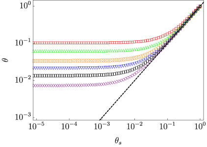
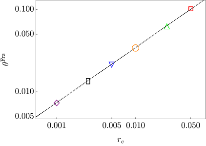
Figure 1: (Left) Dynamical evolution of the granular temperature $\theta$ as a function of the bath temperature $\theta_{\text{s}}$. The different curves correspond to DSMC simulation data for the linear cooling protocol (III.1) with different rates $r_{c}$, namely: $r_{c}$= 0.05 (red squares), $0.025$ (green up triangles), $0.01$ (orange circles), $0.005$ (blue down triangles), $0.0025$ (black rectangles), and $0.001$ (purple diamonds). The black dashed line corresponds to the instantaneous NESS curve $\theta=\theta_{\text{s}}$. (Right) Limit values of the kinetic temperature at the frozen state as a function of the cooling rate. The plotted points have been extracted from the DSMC data on the left panel. The black, dotted line corresponds to the best fit of those points to the function $a\,r_{c}^{b}$, with $a=0.741$ and $b=0.666$, in excellent agreement with the theoretical prediction (III.11).

Let us now compare our analytical predictions with simulation results obtained from Direct Simulation Monte Carlo (DSMC) integration[bird_g_a_molecular_1994] of the kinetic equation that governs the dynamics of the granular gas. Unless otherwise specified, for all of the simulations of the granular gas performed, we have employed the system parameters $\alpha=0.9$, $d=3$, and a number of particles $N=10^{5}$. On the left panel of Fig. 1, we plot the relaxation of the kinetic temperature when applying the cooling programme from Eq.(III.1). The final granular temperatures $\theta^{\text{Frz}}$ at the frozen state are plotted on the right panel versus the cooling rate $r_{c}$. They are very well fitted by the power law $\theta^{\text{Frz}}=a\,r_{c}^{b}$ with $b=0.666$, thus confirming the scaling given by Eq. (III.11).

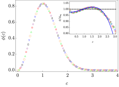
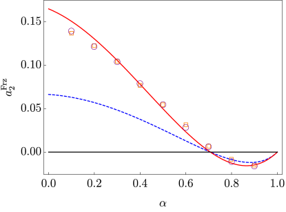
Figure 2: Universality of the frozen state. (Left) VDF at the frozen state for different values of the cooling rate $r_{c}$. The curves have been obtained from the same numerical data employed for Fig. 1, for which $\alpha=0.9$ and $d=3$, and thus the colour code and associated symbols are the same. All VDFs are superimposed over a unique, universal, curve independent of $r_{c}$, in agreement with our theoretical prediction. In the inset, we show the VDF at the frozen state divided by the equilibrium Maxwellian, with the solid line corresponding to the polynomial in Eq. (II.4) within the first Sonine approximation. (Right) Excess kurtosis at the frozen state as a function of the restitution coefficient $\alpha$. Here, for the sake of clarity, we show DSMC data corresponding to only two values of the cooling rate, $r_{c}=0.01$ (squares) and $r_{c}=0.001$ (circles). The numerical values of the excess kurtosis at the frozen state are compared with both the NESS value $a_{2}^{\text{s}}$ (blue dashed line) and the HCS value $a_{2}^{\text{HCS}}$ (red solid line), being very close to the latter.

In Fig. 2, we prove that the frozen state is indeed unique. On the left panel, the dimensionless VDF at the frozen state corresponding to different cooling rates overlap on a universal curve. Note that, although our theoretical analysis has been carried out within the first Sonine approximation, the numerical results show that this remarkable property holds for the exact (numerical) VDF. To neatly visualise the non-Gaussian character of the frozen state, we present (i) the ratio of the VDF over the equilibrium Maxwellian in the inset of the left panel and (ii) the excess kurtosis at the frozen state $a_{2}^{\text{Frz}}$ as a function of the restitution coefficient $\alpha$ on the right panel. This also allows us to check that $a_{2}^{\text{Frz}}$—and thus the VDF—is indeed independent of $r_{c}$ for all inelasticities. The graph shows that $a_{2}^{\text{Frz}}$ is really far from the steady-state kurtosis $a_{2}^{\text{s}}$ but very close to the HCS values $a_{2}^{\text{HCS}}$, which suggests that the HCS has a key role in the frozen state—as further discussed in Appendix A.

III.2 Boundary layer approach. Universality

We are now concerned with the behaviour of the system for very low bath temperatures, when the system is close to its frozen state. We follow a boundary layer approach, in which we introduce scaled variables and look for a distinguished limit of the evolution equations (II.10). In this way, we find an inner expansion, valid for low temperatures, which is afterwards matched with the outer solution derived above: in this way, an (approximate) solution for all values of the bath temperature, known as a uniform solution,[bender_advanced_1999] is built.

We define the scaled variables

$$Y\equiv r_{c}^{-2/3}\theta,\quad X\equiv r_{c}^{-2/3}\theta_{\text{s}},$$ (III.13)

as suggested by Eqs. (III.11) and (III.12). Interestingly, the evolution equations (II.10) become independent of the cooling rate when written in terms of $X$ and $Y$:

$$-\frac{dY}{dX} =X^{3/2}\left(1+\frac{3}{16}a_{2}^{\text{s}}\right)-Y^{3/2}\left(1+\frac{3}{16}a_{2}\right),$$ (III.14a)

$$-\frac{da_{2}}{dX} =2Y^{1/2}\left\{\left[1-\left(\frac{X}{Y}\right)^{3/2}\right]a_{2}+B\,(a_{2}^{\text{s}}-a_{2})\right\}.$$ (III.14b)

These equations provide us with the inner solution, which is expected to be valid for $(X,Y,a_{2})$ of the order of unity, i.e. close to the frozen state as discussed above. In order to find the inner solution, we must complement Eq. (III.14) with the boundary conditions (III.4), which are now written as

$$Y(r_{c}^{-2/3})=r_{c}^{-2/3},\quad a_{2}(r_{c}^{-2/3})=a_{2}^{\text{s}}.$$ (III.15)

Note that the boundary conditions have absorbed all the dependency of the inner solution on the cooling rate $r_{c}$.

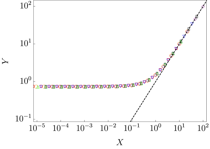
Figure 3: Plot of the dynamical evolution of the scaled granular temperature $Y$ as a function of $X$ using the cooling protocol (III.1) for different cooling rates. The colour codes and symbols for the DSMC data are the same as those for the data depicted in Fig.1.

Figure 3 shows the same numerical data on the left panel of Fig. 1, obtained from DSMC simulation, but in terms of the scaled variables $X$ and $Y$. It is neatly observed that all the curves for different values of the cooling rate $r_{c}$ collapse onto a unique master curve, independent of $r_{c}$. The only difference appears for large values of $X$, for which the different curves start from different initial points, consistently with the boundary conditions (III.15). Since the plotted data corresponds to the numerical solution to the kinetic equation, not to our perturbative approach, this suggests that the exact solution to the problem presents a universal behaviour in scaled variables.

In order to understand such universal behaviour in scaled variables, we seek the solution of the inner problem at the lowest order, which we denote by $(Y_{I}(X),a_{2,I}(X))$. Therefore, we have to solve Eq. (III.14) with the approximate boundary conditions at infinity

$$\lim_{X\to\infty}Y_{I}(X)=\infty,\quad\lim_{X\to\infty}a_{2,I}(X)=a_{2}^{\text{s}},$$ (III.16)

which are obtained by considering the limit as $r_{c}\to 0$ in Eq. (III.15). Although it is not possible to write $(Y_{I}(X),a_{2,I}(X))$ in a simple closed form, it is clear that $(Y_{I}(X),a_{2,I}(X))$ does not depend on $r_{c}$, since the dependence thereof has vanished in Eq. (III.16). A dominant balance of Eq. (III.14) shows that

$$Y_{I}(X)\sim X,\qquad a_{2,I}(X)\sim a_{2}^{\text{s}},\quad X\gg 1,$$ (III.17)

which is consistent with the tendency of the DSMC data in Fig. 3 to the NESS curve (dashed line) for large $X$.

It can be shown that the above universality also holds for the uniform solution—valid over the whole interval of $\theta_{\text{s}}$, not only for low temperatures. The uniform solution is constructed as the sum of the outer and inner solutions, minus the common behaviour found in the intermediate matching region, where $\theta_{\text{s}}\ll 1$ but $X\gg 1$.[bender_advanced_1999] That is, the uniform solution to the lowest order can be written as

$$\theta_{\text{BL}}(\theta_{\text{s}}) =\theta_{O}(\theta_{\text{s}})+r_{c}^{2/3}Y_{I}(X=r_{c}^{-2/3}\theta_{\text{s}})-\theta_{c}(\theta_{\text{s}}),$$ (III.18)

$$a_{2,\text{BL}}(\theta_{\text{s}}) =a_{2,O}(\theta_{\text{s}})+a_{2,I}(X=r_{c}^{-2/3}\theta_{\text{s}})-a_{2,c}(\theta_{\text{s}}).$$ (III.19)

The common behaviour for the kinetic temperature and the excess kurtosis are

$$\theta_{c}(\theta_{\text{s}})=\theta_{\text{s}},\quad a_{2,c}(\theta_{\text{s}})=a_{2}^{\text{s}},$$ (III.20)

bringing to bear Eqs. (III.10) and (III.17). Note that the common behaviour coincides with the outer solution (III.10), so the uniform solution coincides with the inner solution and its range of validity extends to all values of $X$,

$$\theta_{\text{BL}}(\theta_{\text{s}}) =r_{c}^{2/3}Y_{I}(X=r_{c}^{-2/3}\theta_{\text{s}}),$$ (III.21)

$$a_{2,\text{BL}}(\theta_{\text{s}}) =a_{2,I}(X=r_{c}^{-2/3}\theta_{\text{s}}).$$ (III.22)

The first equation tells us that $Y_{\text{BL}}\equiv r_{c}^{-2/3}\theta_{\text{BL}}=Y_{I}$, i.e. we have the universal behaviour in Fig. 3 over the uniform solution—at the lowest order.

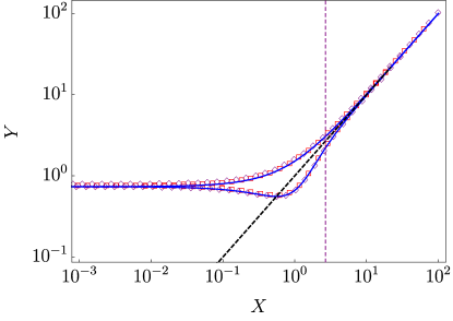
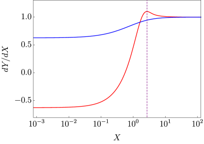
Figure 4: Hysteresis cycle upon reheating in the granular gas. (Left) Kinetic temperature as a function of the bath temperature, when the latter is first cooled down with rate $r_{c}$ and later reheated from the frozen state with rate $r_{h}=r_{c}=r$. Specifically, we present results for $r=0.01$ (red squares) and $r=0.001$ (purple diamonds). Symbols are simulation results of the kinetic equation, while the blue solid curves correspond to the numerical integration of Eqs. (III.14) and (IV.2). The black dashed straight line corresponds to the NESS curve $Y=X$. (Right) Associated apparent heat capacity $dY/dX$. The red (blue) line corresponds to the heating (cooling) programme, specifically to the numerical integration of Eqs. (III.14) and (IV.2). The purple vertical line marks the bath temperature $X_{g}$ at which the heat capacity reaches its maximum in the reheating programme.

From the boundary layer solution, the frozen values of the scaled variables are readily obtained,

$$Y^{\text{Frz}} \equiv\lim_{X\to 0}Y_{\text{I}}(X),$$ (III.23a)

$$a_{2}^{\text{Frz}} \equiv\lim_{X\to 0}a_{2,\text{I}}(X).$$ (III.23b)

Our above argument about the independence of $Y_{I}(X)$ on the cooling rate is immediately translated to $\theta_{\text{Frz}}=r_{c}^{2/3}Y^{\text{Frz}}$, which means that $\theta_{\text{Frz}}$ follows the power law behaviour $\theta_{\text{Frz}}\propto r_{c}^{2/3}$ that we have already checked on the right panel of Fig. 1. Also, the independence of $a_{2,I}(X)$ on the cooling rate, and thus the independence of $a_{2}^{\text{Frz}}$ on $r_{c}$ has been already checked on the right panel of Fig. 2.

IV Hysteresis cycles

Now we turn our attention to a reheating protocol from the frozen state with rate $r_{h}$, $d\theta_{\text{s}}/dt=+r_{h}$. First, we consider the paradigmatic case $r_{h}=r_{c}$. Even in this simple case, we will show that the system does not follow backwards the cooling curve, but crosses the NESS line $\theta=\theta_{\text{s}}$ and afterwards tends thereto from below. This is similar to the hysteresis cycle displayed by glassy systems in temperature cycles (cooling followed by reheating). Second, we consider the more general case $r_{h}\neq r_{c}$, in particular we are interested in analysing the reheating with a given rate $r_{h}$ after the system has been cooled down to different frozen states corresponding to different values of $r_{c}$.

IV.1 Universal hysteresis cycle with $r_{c}=r_{h}$

Similarly to the cooling programme, we may introduce scaled variables as

$$Y\equiv r_{h}^{-2/3}\theta,\quad X\equiv r_{h}^{-2/3}\theta_{\text{s}}.$$ (IV.1)

In terms thereof, the evolution equations become independent of the heating rate,

$$\frac{dY}{dX} =X^{3/2}\left(1+\frac{3}{16}a_{2}^{\text{s}}\right)-Y^{3/2}\left(1+\frac{3}{16}a_{2}\right),$$ (IV.2a)

$$\frac{da_{2}}{dX} =2\sqrt{Y}\left[\left(1-\left(\frac{X}{Y}\right)^{3/2}\right)a_{2}+B\,(a_{2}^{\text{s}}-a_{2})\right].$$ (IV.2b)

The above system must be complemented with the new boundary conditions

$$Y(0)=Y^{\text{Frz}},\quad a_{2}(0)=a_{2}^{\text{Frz}},$$ (IV.3)

which correspond to that of the frozen state from the previously applied cooling programme, given by Eq.(III.23) to the lowest order—recall that $r_{c}=r_{h}$.

A completely similar analysis to that carried out for the cooling programme shows that the solution to Eq. (IV.2) gives the lowest order approximation to the behaviour of the kinetic temperature and the excess kurtosis in the heating programme. Since the rate $r_{c}=r_{h}$ does not appear in these equations, the reheating behaviour is also independent of the rate: there is a unique, universal, hysteresis cycle for all rates.

The above theoretical prediction is checked in Fig. 4. On the left panel, the hysteresis cycle of the kinetic temperature is shown. DSMC simulation data (symbols) are compared with the boundary layer solution (blue lines) of Eq. (IV.2), for different values of the cooling/heating rate $r=r_{c}=r_{h}$. The independence of $r$ of the hysteresis cycle is clearly observed, and the boundary layer solution captures very well the numerical results throughout the whole cycle. Remarkably, the heating curve crosses the NESS line $\theta=\theta_{\text{s}}$ (black dashed line) and tends thereto from below—this is further analysed in Sec. IV.2. On the right panel, we display the apparent “heat capacity" $d\theta/d\theta_{\text{s}}=dY/dX$ over the thermal cycle. This heat capacity is non-monotonic in the heating process, with a marked maximum at a certain value of $\theta_{\text{s}}$ (or $X$) that can be employed to define the glass transition temperature $\theta_{\text{s},g}$ (or $X_{g}$).[brey_dynamical_1994, angell_formation_1995, dyre_colloquium_2006, tropin_modern_2016, richet_thermodynamics_2021]

IV.2 Normal heating curve

In order to understand the hysteretic behaviour, a perturbative approach to the heating process can be carried out by expanding the granular temperature $\theta$ in powers of $r_{h}$, similarly as we did for the cooling process. By simply changing $r_{c}\leftrightarrow-r_{h}$, we obtain the perturbative expressions

$$\theta =\theta_{\text{s}}-\frac{2}{3}\frac{r_{h}}{\theta_{\text{s}}^{1/2}}\left[1+\frac{3}{16}\;a_{2}^{\text{s}}\left(1+\frac{1}{B}\right)\right]^{-1}+O(r_{h}^{2}),$$ (IV.4a)

$$a_{2} =a_{2}^{\text{s}}+\frac{r_{h}\ a_{2}^{\text{s}}}{B\;\theta_{\text{s}}^{3/2}}\left[1+\frac{3}{16}\;a_{2}^{\text{s}}\left(1+\frac{1}{B}\right)\right]^{-1}+O(r_{h}^{2}).$$ (IV.4b)

These perturbative expressions are expected to be valid for not too low temperatures, i.e. over the outer layer—employing the terminology of boundary layer theory. Note that they depend on the heating programme $r_{h}$, but not on the previously applied cooling programme with cooling rate $r_{c}$. In other words, if we start the heating process from different initial frozen temperatures $\theta^{\text{Frz}}=Y^{\text{Frz}}r_{c}^{2/3}$ corresponding to different values of $r_{c}$ but reheat with a common rate $r_{h}$, we expect to approach the behaviour in Eq. (IV.4) once the system reaches the outer layer. That is the behaviour depicted in Fig. 5: despite having different cooling programmes, all the simulation results tend to reach a universal curve for high enough values of the bath temperature.

The above behaviour is similar to that found in simple systems described by master equations, in which it can be analytically proved that there exists a universal normal curve in the heating case that is the global attractor of the dynamics.[brey_normal_1993, brey_dynamical_1994, brey_dynamical_1994-1, prados_hysteresis_2000, prados_glasslike_2001] In this context, the expressions in Eq. (IV.4) may be considered as perturbative expansions of a similar normal curve in the granular gas. Equation (IV.4a) explains why the kinetic temperature overshoots the NESS curve $\theta=\theta_{\text{s}}$ in reheating, which stems from the normal curve lying below the NESS curve—whereas the cooling curves always lie above the NESS curve, as illustrated by Fig. 1.

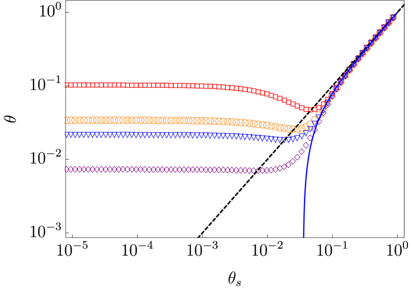
Figure 5: Hysteresis cycles for reheating with rate $r_{h}$ from the frozen states corresponding to different cooling rates $r_{c}$. Reheating curves for the kinetic correspond to $r_{h}=0.01$, and the different cooling rates employed are: (colour, $r_{c}$) = (red, $0.05$), (orange, $0.01$), (blue, $0.005$) and (purple, $0.001$). Symbols correspond to DSMC simulation data, whereas the blue solid curve corresponds to the perturbative expression for the normal curve in Eq. (IV.4).

V Molecular fluid with non-linear drag

We now focus our attention to a second relevant physical system: a molecular fluid with non-linear drag.[klimontovich_statistical_1995, lindner_diffusion_2007, santos_mpemba_2020, patron_strong_2021, goychuk_nonequilibrium_2021] The considered model arises when analysing an ensemble of Brownian particles of mass $m$ immersed in an isotropic and uniform background fluid,[ferrari_particles_2007, ferrari_particles_2014] the particles of which have mass $m_{\text{bf}}$. In the $m_{\text{bf}}/m\to 0$ limit—the so-called Rayleigh limit, the drag coefficient $\zeta$ becomes velocity independent and thus the drag force is linear. However, in real physical scenarios we have that $m_{\text{bf}}/m\neq 0$, and it is thus relevant to consider the corrections to the Rayleigh limit. Specifically, by introducing the first order corrections thereto, i.e. by retaining only linear terms in $m_{\text{bf}}/m$, the drag coefficient is found to be quadratic on the velocities.[ferrari_particles_2007, ferrari_particles_2014, hohmann_individual_2017] Interestingly, it has recently been shown that this model describes a mixture of ultracold Cs and Rb atoms.[hohmann_individual_2017]

Let us consider a system of $d$-dimensional hard spheres of mass $m$, diameter $\sigma$, and density $n$ immersed in a background fluid at temperature $T_{\text{s}}$. In the regime just explained above, the Brownian particles are subjected to a non-linear drag force of the form[ferrari_particles_2007, ferrari_particles_2014, hohmann_individual_2017]

$$\bm{F}=-m\,\zeta(v)\bm{v},$$ (V.1)

where $\bm{v}$ is the particle velocity, and

$$\zeta(v)=\zeta_{0}\Big{(}1+\gamma\frac{mv^{2}}{k_{B}T_{\text{s}}}\Big{)}$$ (V.2)

is a non-linear drag coefficient, with $\gamma$ being a dimensionless parameter that measures the degree of non-linearity of the drag force, and $\zeta_{0}$ is the zero-velocity limit of the drag coefficient. The latter depends on the bath temperature $T_{\text{s}}$; for hard spheres, it is found that $\zeta_{0}\propto T_{\text{s}}^{1/2}$—see e.g. Refs. hohmann_individual_2017, santos_mpemba_2020 for the complete expression. The dependence of $\zeta_{0}$ on $T_{\text{s}}$ is relevant here because the bath temperature depends on time in cooling/heating processes.

Similarly to the granular gas, the system may be accurately described by the one-particle VDF $f(\bm{v},t)$ if sufficiently diluted. In this case, the dynamical evolution of the VDF is governed by the Fokker-Planck equation (FPE)

$$\partial_{t}f(\bm{v},t)-\frac{\partial}{\partial\bm{v}}\cdot\left[\zeta(v)\bm{v}+\frac{\xi^{2}(v)}{2}\frac{\partial}{\partial\bm{v}}\right]f(\bm{v},t)=0,$$ (V.3)

where $m^{2}\xi^{2}(v)$ is the variance of a stochastic white noise force. The coefficients $\xi^{2}(v)$ and $\zeta(v)$ are related by means of the fluctuation-dissipation relation

$$\xi^{2}(v)=\frac{2k_{B}T_{s}}{m}\zeta(v),$$ (V.4)

which ensures that the equilibrium Maxwellian VDF

$$f_{s}(\bm{v})=n\left(\frac{m}{2\pi k_{B}T_{s}}\right)^{\frac{d}{2}}e^{-\frac{mv^{2}}{2k_{B}T_{s}}},$$ (V.5)

constitutes the unique stationary solution of the FPE (V.3).

The velocity dependence of the drag coefficient implies that we have multiplicative noise in this problem.[van_kampen_stochastic_1992, gardiner_stochastic_2009] By employing the Ito interpretation of stochastic integration[van_kampen_ito_1981, mannella_ito_2012], which is the most convenient one for numerical simulations, the FPE is equivalent to the following Langevin equation:

$$\dot{\bm{v}}(t)=-\zeta_{\rm{eff}}(v)\,\bm{v}(t)+\xi(v)\,\bm{\eta}(t),$$ (V.6)

where

$$\zeta_{\rm{eff}}(v)=\zeta_{0}\Big{(}1-2\gamma+\gamma\frac{mv^{2}}{k_{B}T_{\text{s}}}\Big{)}$$ (V.7)

constitutes an effective drag coefficient, while $\bm{\eta}(t)$ is a Gaussian white noise of zero average $\langle\bm{\eta}(t)\rangle=0$ and correlations $\langle\eta_{i}(t)\,\eta_{j}(t^{\prime})\rangle=\delta_{i,j}\,\delta(t-t^{\prime})$.

The kinetic temperature is again defined as in Eq. (II.2) for the granular gas, but understanding $f(\bm{v},t)$ as the solution of the FPE. Inserting (II.2) into (V.3) leads to the following evolution equation for the temperature,

$$\dot{T}=\zeta_{0}\;\biggl{\{} 2(T_{\text{s}}-T)\left[1+\gamma(d+2)\frac{T}{T_{\text{s}}}\right]$$

$$-2\gamma(d+2)\frac{T^{2}}{T_{\text{s}}}a_{2}\biggr{\}},$$ (V.8)

where $a_{2}$ corresponds to the excess kurtosis, previously introduced in Eq. (II.5) when studying the granular gas.

For non-linear drag, $\gamma\neq 0$, the evolution of the temperature is coupled to that of the excess kurtosis and, thus, we need to consider the evolution equation for the latter too. In turn, the evolution equation for the excess kurtosis involves sixth-degree moments, and in general there emerge an infinite hierarchy of equations for the moments. Under the first Sonine approximation, we have the evolution equations[santos_mpemba_2020, patron_strong_2021]

$$\dot{\theta}=\theta_{\text{s}}^{1/2}\,\bigg{[} 2(\theta_{\text{s}}-\theta)+2\gamma(d+2)\,\theta$$

$$-2\,\gamma\,(d+2)(1+a_{2})\frac{\theta^{2}}{\theta_{\text{s}}}\bigg{]},$$ (V.9a)

$$\dot{a}_{2}=\theta_{\text{s}}^{1/2}\;\biggl{\{} 8\gamma\left(1-\frac{\theta}{\theta_{\text{s}}}\right)$$

$$-\left[\frac{4\theta_{\text{s}}}{\theta}-8\gamma+4\gamma(d+8)\frac{\theta}{\theta_{\text{s}}}\right]a_{2}\biggr{\}},$$ (V.9b)

where we have introduced the dimensionless variables

$$\theta\equiv\frac{T}{T_{i}},\quad\theta_{\text{s}}\equiv\frac{T_{\text{s}}}{T_{i}},\quad t^{*}\equiv\zeta_{0}(T_{i})\;t,$$ (V.10)

with $T_{i}\equiv T(t=0)$ being the initial temperature. We have also taken into account that $\zeta_{0}(T_{\text{s}})=\zeta_{0}(T_{i})\theta_{\text{s}}^{1/2}$.

In previous work,[patron_strong_2021, patron_nonequilibrium_2023] we have shown that the non-linear fluid approaches a non-equilibrium state, termed LLNES (long-lived non-equilibrium state), over a wide intermediate timescale, when instantaneously quenched to low enough values of the bath temperature, i.e. $T_{i}/T_{\text{s}}\gg 1$. The VDF at the LLNES is given by a delta peak; in terms of the scaled variables in Eq. (II.3), it reads

$$\phi_{\text{L}}(\bm{c})=\Omega_{d}^{-1}\left(\frac{2}{d}\right)^{\frac{d-1}{2}}\delta\left(c-\sqrt{\frac{d}{2}}\right),$$ (V.11)

with $\Omega_{d}$ being the $d$-dimensional solid angle.[patron_nonequilibrium_2023] The exact value of the excess kurtosis at the LLNES will be useful, which is

$$a_{2}^{\text{L}}=-\frac{2}{d+2}.$$ (V.12)

It is worth remarking that the VDF for the LLNES, and thus $a_{2}^{\text{L}}$, does not depend on the non-linearity parameter $\gamma$.[patron_nonequilibrium_2023]

The LLNES state corresponds to the extreme scenario that comes about when the system is instantaneously quenched to a very low temperature. In this case, for a system relaxing from equilibrium at $T_{i}$ to equilibrium at $T_{\text{s}}\ll T_{i}$, the system first reaches the LLNES and afterwards tends to equilibrium from it. Note the strong similarity with the HCS for granular gases, which also appears when the intensity of the stochastic thermostat is instantaneously quenched to a very low value. In such a protocol, the granular gas first approaches the HCS and afterwards tends to the stationary state imposed by the stochastic thermostat. Thus, it is worth investigating the role played by the LLNES in the possible emergence of a laboratory glass transition in fluids with non-linear drag.

VI Glassy behaviour of the non-linear molecular fluid

Now, in order to investigate a possible glass transition in the molecular fluid, we decrease the bath temperature following the same cooling programme as in Eq. (III.1) for the granular gas. In fact, as we follow the same perturbative approach in the cooling rate, we leave the mathematical details for Appendix B. Up to order $O(r_{c})$, the regular perturbative solution is given by

$$\theta =\theta_{\text{s}}+\frac{r_{c}}{2\theta_{\text{s}}^{1/2}}\,\frac{1+\gamma(d+6)}{\left[1+\gamma(d+4)\right]^{2}-2\gamma^{2}(d+4)},$$ (VI.1a)

$$a_{2} =-\frac{r_{c}}{\theta_{\text{s}}^{3/2}}\frac{\gamma}{\left[1+\gamma(d+4)\right]^{2}-2\gamma^{2}(d+4)}.$$ (VI.1b)

Thus, we have that $\theta-\theta_{\text{s}}\propto r_{c}/\theta_{\text{s}}^{1/2}$ and $a_{2}\propto r_{c}/\theta_{\text{s}}^{3/2}$. Our regular perturbative approach fails when the $O(r_{c}^{0})$ and the $O(r_{c}^{1})$ terms become comparable, i.e. again when $\theta_{\text{s}}=O(r_{c}^{2/3})$, which implies that $\theta=O(r_{c}^{2/3})$ and $a_{2}=O(1)$. Let us outline that, regardless of the intrinsic differences between the molecular fluid and granular gas systems, they both lead to the same scaling for both the kinetic temperature and the excess kurtosis.

The above discussion entails the necessity of introducing again a boundary layer approach. We define scaled variables, analogous to those for the granular gas in Eq. (III.13), $Y\equiv r_{c}^{-2/3}\theta$ and $X\equiv r_{c}^{-2/3}\theta_{\text{s}}$. In term of the scaled variables, the evolution equations (II.10) become independent of $r_{c}$,

$$-\frac{dY}{dX}= X^{1/2}\,\bigg{\{}2\,(X-Y)\left[1+\gamma(d+2)\frac{Y}{X}\right]$$

$$-2\gamma(d+2)\frac{Y^{2}}{X}a_{2}\bigg{\}},$$ (VI.2a)

$$-\frac{da_{2}}{dX}= X^{1/2}\left\{8\gamma\left(1-\frac{Y}{X}\right)\right.$$

$$\left.-\left[\frac{4X}{Y}-8\gamma+4\gamma(d+8)\frac{Y}{X}\right]a_{2}\right\},$$ (VI.2b)

as all the dependence on $r_{c}$ is being absorbed in the boundary conditions

$$Y(r_{c}^{-2/3})=r_{c}^{-2/3},\quad a_{2}(r_{c}^{-2/3})=0.$$ (VI.3)

It is clear the resemblance of the found picture and that of our previous study of the granular gas. Therefore, in order to avoid reiteration, we focus on the main aspects of the glassy behaviour in the molecular fluid. As will be seen, the analogy with the behaviour found in the granular gas is almost complete.

The lowest order solution for the cooling protocol would be again obtained by solving Eqs. (VI.2) with the boundary conditions $\lim_{X\to\infty}Y(X)=\infty$, $\lim_{X\to\infty}a_{2}(X)=0$, which is completely independent of $r_{c}$. At the frozen state we thus have

$$Y^{\text{Frz}}\equiv\lim_{X\to 0}Y(X),\quad a_{2}^{\text{Frz}}\equiv\lim_{X\to 0}a_{2}(X),$$ (VI.4)

which are expected to be independent of $r_{c}$. We check this expectation in Table 1, in which we compare the value of $Y^{\text{Frz}}$ and $a_{2}^{\text{Frz}}$ obtained from numerical simulation of the Langevin equation (V.6), for different values of $r_{c}$, and our theoretical prediction. The agreement is excellent for the kinetic temperature, and fair for the excess kurtosis. This was to be expected within the first Sonine approximation since $a_{2}^{\text{Frz}}$ is quite large for the non-linear fluid. Moreover, $a_{2}^{\text{Frz}}$ is not so close to its value at the LLNES, $a_{2}^{\text{L}}=-0.4$ for $d=3$ as predicted by Eq. (V.12), as it was $a_{2}^{\text{Frz}}$ close to its HCS value in the granular gas. See Appendix A for a more detailed discussion on this point.

	$Y^{\text{Frz}}$	$a_{2}^{\text{Frz}}$
Boundary layer	0.397	-0.154
Sim. ($r_{c}=0.05$)	0.402	-0.146
Sim. ($r_{c}=0.01$)	0.403	-0.147
Sim. ($r_{c}=0.005$)	0.403	-0.144
Sim. ($r_{c}=0.001$)	0.404	-0.148

Table 1: Comparison between the numerical (simulation) and theoretical (boundary layer) values of the scaled kinetic temperature and the excess kurtosis at the frozen state. Specifically, we have considered a three-dimensional non-linear fluid with non-linearity parameter $\gamma=0.1$.

The independence of $a_{2}^{\text{Frz}}$ on the cooling rate suggests that this property should also hold for the complete VDF of the non-linear fluid—as was the case for the granular gas. We check this property by plotting the scaled VDF for the non-linear fluid on the frozen state, obtained from the numerical integration of the Langevin equation (V.6), in Fig. 6. The universality of the VDF at the frozen state is clearly observed. The largeness of $a_{2}^{\text{Frz}}$ entails that the deviation from the Maxwellian equilibrium distribution is also large. For reference, the position of the delta peak corresponding to the LLNES is also plotted.

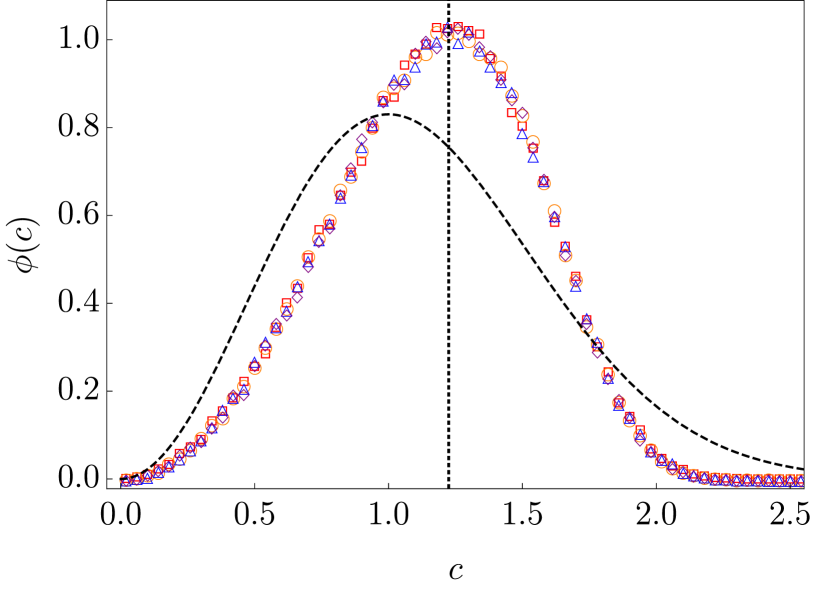
Figure 6: Plot of the dimensionless VDF at the frozen state for the non-linear fluid. Symbols correspond to the numerical integration of the Langevin equation for $N=10^{5}$ stochastic trajectories for different cooling rates: $r_{c}=0.005$ (purple diamonds), $0.01$ (blue triangles), $0.05$ (orange circles) and $0.1$ (red squares). The black dashed curve corresponds to the equilibrium Maxwellian, whereas the vertical line marks the position of the Dirac-delta peak at the LLNES, as given by Eq. (V.11). Other parameters are $\gamma=0.1$, $d=3$.

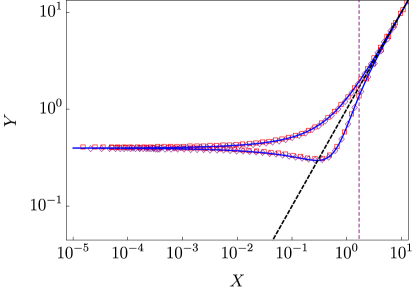
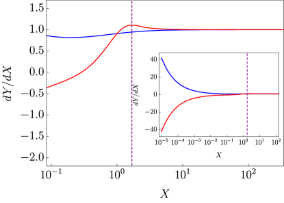
Figure 7: Hysteresis cycle in the non-linear molecular fluid. Both panels are the transposition to case of the non-linear molecular fluid of those in Fig. 4 for the granular gas, with the same values of the cooling and heating rate $r$ in dimensionless variables. For the molecular fluid, the numerical data corresponds to the simulation of the Langevin equation (V.6), while the theoretical curves correspond to the numerical integration of Eqs. (VI.2) and (VI.5). Other parameters employed are $\gamma=0.1$ and $d=3$. On the right panel, there is an additional inset to show the anomalous behaviour of the apparent heat capacity in the cooling process, which is discussed in the text.

From the frozen state, we may reheat the system with the same rate $r_{h}=r_{c}$. Once more, scaled variables are introduced as $Y\equiv r_{h}^{-2/3}\theta$ , $X\equiv r_{h}^{-2/3}\theta_{\text{s}}$, and the evolution equations become independent of the heating rate

$$\frac{dY}{dX}= X^{1/2}\,\bigg{\{}2\,(X-Y)\left[1+\gamma(d+2)\frac{Y}{X}\right]$$

$$-2\gamma(d+2)\frac{Y^{2}}{X}a_{2}\bigg{\}},$$ (VI.5a)

$$\frac{da_{2}}{dX}= X^{1/2}\left\{8\gamma\left(1-\frac{Y}{X}\right)\right.$$

$$\left.-\left[\frac{4X}{Y}-8\gamma+4\gamma(d+8)\frac{Y}{X}\right]a_{2}\right\},$$ (VI.5b)

which differ from the cooling evolution equations (VI.2) only in the sign of the left hand side (lhs). Again, this system has to be solved with the boundary conditions $Y(0)=Y^{\text{Frz}}$, $a_{2}(0)=a_{2}^{\text{Frz}}$, which correspond to the frozen state from the previously applied cooling programme.

Figure 7 is the transposition of Fig. 4 to the case of the non-linear molecular fluid. Its left panel shows both the numerical simulations of the Langevin equation (red symbols) and the boundary layer solution (blue lines) for a full hysteresis cycle. Similarly to the granular gas case, our boundary layer solution captures very well the simulation data. On the right panel, the behaviour of the associated apparent heat capacity of the molecular fluid, $d\theta/d\theta_{\text{s}}=dY/dX$ is displayed. In the reheating curve, the typical maximum that may be used to define a glass transition temperature is neatly observed. Interestingly, in the cooling curve, an anomalous behaviour emerges, the apparent heat capacity increases instead of going to a constant. This anomalous behaviour is better discerned in the inset—which shows a zoom of the very low temperatures region. This stems from the singular behaviour for small $X$ of the dynamic equation  (VI.2a) for $Y$ in the cooling protocol: therefrom, one has that

$$\frac{dY}{dX} \sim 2\gamma(d+2)\frac{(Y^{\text{Frz}})^{2}}{X^{1/2}}(1+a_{2}^{\text{Frz}}),\quad X\ll 1,$$ (VI.6)

which diverges as $X^{-1/2}$. This has to be contrasted with the behaviour for the granular gas: from Eq. (III.14a), one has that in the cooling protocol

$$\frac{dY}{dX}\sim(Y^{\text{Frz}})^{3/2}\left(1+\frac{3}{16}a_{2}^{\text{Frz}}\right),\quad X\ll 1,$$ (VI.7)

which goes to a constant—consistently with the behaviour reported in Fig. 4.

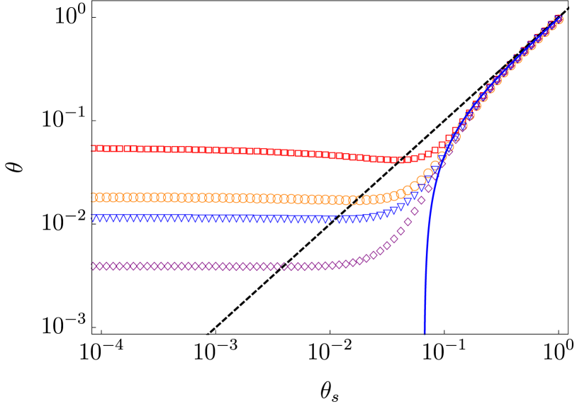
Figure 8: Heating curves for the kinetic temperature with heating rate $r_{h}=0.05$, that have been previously cooled towards their frozen values with different cooling rates: (colour, $r_{c}$) = (red, $0.05$), (orange, $0.01$), (blue, $0.005$), and (purple, $0.001$). Symbols are simulation results while the blue solid curve corresponds to the perturbative solution from Eq. (VI.8). Other parameters are $\gamma=0.1$ and $d=3$.

Finally, our molecular fluid also presents an universal curve when reheated from different frozen states. A regular perturbation theory, once more analogous to that carried out before for the granular gas, gives

$$\theta =\theta_{\text{s}}-\frac{r_{h}}{2\theta_{\text{s}}^{1/2}}\,\frac{1+\gamma(d+6)}{\left[1+\gamma(d+4)\right]^{2}-2\gamma^{2}(d+4)},$$ (VI.8a)

$$a_{2} =+\frac{r_{h}}{\theta_{\text{s}}^{3/2}}\frac{\gamma}{\left[1+\gamma(d+4)\right]^{2}-2\gamma^{2}(d+4)},$$ (VI.8b)

neglecting $O(r_{h}^{2})$ terms. These expressions are obtained from Eqs. (VI.1) by exchanging $r_{c}\leftrightarrow-r_{h}$. They are valid for the return to the equilibrium curve, when the system is close enough thereto—i.e. for high enough temperatures; more specifically, when $\theta_{\text{s}}\gtrsim r_{h}^{2/3}$. Therefore, if the system is reheated from different initial frozen states with kinetic temperatures $\theta^{\text{Frz}}=Y^{\text{Frz}}r_{c}^{2/3}$, obtained from previously applied cooling programmes with different rates $r_{c}$, we expect the kinetic temperature to tend towards Eq. (VI.8a) as $\theta_{\text{s}}$ increases. This entails the behaviour shown in Fig. 8: all the heating curves, independently of the previous cooling rate $r_{c}$, overshoot the equilibrium curve and tend towards a unique curve when being reheated with rate $r_{h}$.

VII Conclusions

We have investigated the emergence of a laboratory glass transition in two basic fluid models: a granular gas of smooth hard spheres and a molecular fluid with non-linear drag force. The two systems are very different from a fundamental point of view. One the one hand, collisions in the granular gas are inelastic, and thus its VDF is always non-Gaussian and the system is intrinsically out-of-equilibrium, tending eventually to a NESS if an energy injection mechanism is introduced. On the other hand, collisions are elastic in the molecular fluid and the system approaches equilibrium, with a Maxwellian VDF, in the long time limit.

In both cases, our analysis have been carried out within the first Sonine approximation of the relevant evolution equation for the VDF: the inelastic Boltzmann equation for the granular gas, the Fokker-Planck equation for the molecular fluid with non-linear drag. Therein, the evolution equation of the kinetic temperature—basically, the average kinetic energy—is found to be coupled with that of the excess kurtosis. The evolution equation of the excess kurtosis is in turn coupled with higher-order cumulants but these are neglected in the first Sonine approximation, since they are assumed to be small.

Despite the profound differences between granular gases and molecular fluids, both systems share some striking similarities in their dynamical behaviour. Specifically, we have studied the evolution of the kinetic temperature when the bath temperature is decreased by applying a linear cooling programme. We have approached the problem by employing a perturbation theory that assumes that the cooling rate is a small parameter. Interestingly, both for the granular gas and the molecular fluid, the boundary layer approach leads to the same scaling behaviour of the kinetic temperature, predicting that it departs from equilibrium at low bath temperatures and freezes in a value that scales as $r_{c}^{2/3}$. This theoretical prediction has been confirmed by our numerical results, DSMC simulations of the inelastic Boltzmann equation for the granular gas and numerical integration of the non-linear Langevin equation for the molecular fluid.

A key point of our approach is the evolution equations becoming independent of the cooling rate when they are written in terms of scaled variables, well-suited for our boundary layer treatment of the problem. This leads to the emergence of universality of the frozen state, in the sense that the VDF—again, both for the granular gas and the non-linear molecular fluid—at the frozen state is independent of the cooling rate.

Moreover, when the system is reheated from this frozen state with the same rate, this universality extends to the whole dynamical evolution. This entails that the observed hysteresis when the systems are submitted to a thermal cycle—first cooling, followed by reheating—is also universal, independent of the rate of variation of the bath temperature. Once more, this theoretical prediction is confirmed by numerical simulations of both systems, and an excellent agreement between the numerical and the theoretical curves have been found.

Another interesting feature of both systems is their tendency to a unique normal curve upon reheating, independent of the previous cooling programme. This behaviour has been theoretically predicted for Markovian systems obeying master equations,[brey_normal_1993] and observed in a variety of simple models for glasses and dense granular systems.[brey_dynamical_1994, brey_dynamical_1994-1, prados_hysteresis_2000, prados_glasslike_2001] It is this tendency to approach the normal curve that explains the overshoot of the NESS—for the granular gas—or equilibrium—for the molecular fluid—curve of the kinetic temperature upon reheating, since the normal curve lies below them whereas the cooling curves lie above them.

In the granular gas, the values of the excess kurtosis at the frozen state are very close to that of the HCS: this hints at the frozen state being strongly related with the HCS. In the non-linear molecular fluid, the value of the excess kurtosis are further from that at the LLNES, so the relation between the frozen state and the LLNES is less clear. Still, it seems that both the HCS for the granular gas and the LLNES for the non-linear fluid play the role of a reference state for the cooling protocol—a first step in this direction is provided in Appendix A, although this point certainly deserves further investigation.

The universality of the frozen state, in the sense of its independence of $r_{c}$ in scaled variables, is an appealing feature of the laboratory glass transition found in this work—both for the smooth granular gas and the molecular fluid with (quadratic) non-linear drag. The possible extension of this property to other systems, for example rough granular fluids[brilliantov_translations_2007, kremer_transport_2014, torrente_large_2019], molecular fluids with more complex non-linearities,[klimontovich_nonlinear_1994, lindner_diffusion_2007, casado-pascual_directed_2018, goychuk_nonequilibrium_2021, patron_strong_2021] or binary mixtures [serero_hydrodynamics_2006, khalil_homogeneous_2014, gomez_gonzalez_mpemba-like_2021, gomez_gonzalez_time-dependent_2021]is an interesting prospect for future work.

Data availability

The Fortran codes employed for generating the data that support the findings of this study, together with the Mathematica notebooks employed for producing the figures presented in the paper, are openly available in the GitHub page of University of Sevilla’s FINE research group.

Appendix A Glass transition for different cooling programmes

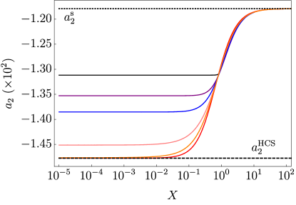
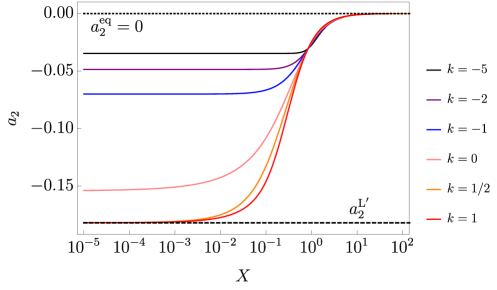
Figure 9: Excess kurtosis $a_{2}$ as a function of the scaled bath temperature $X$ for cooling programmes corresponding to Eq. (A.1) with different values of $k$. (Left) Behaviour found in a granular fluid with parameters $\alpha=0.9$ and $d=3$. (Right) Behaviour found in a molecular fluid with parameters $\gamma=0.1$ and $d=3$. In both cases, a dimensionless cooling rate $r_{c}=0.1$ has been employed, with different values of the parameter $k$. The plotted curves correspond to the numerical integration of the evolution equations in the first Sonine approximation. On the left (right) panel, the black dotted line represents the value of the excess kurtosis at the NESS $a_{2}^{\text{s}}$ (equilibrium value of the excess kurtosis $a_{2}^{\text{eq}}=0$), from which all the curves depart for large $X$, whereas the black dashed line accounts for the value at the HCS (LLNES) within the first Sonine approximation.

Throughout this work, we have employed linear cooling programmes in order to study the emergence of glassy behaviour in both molecular fluids and granular gases. Let us now consider the following more general family of cooling protocols,

$$\frac{d\theta_{\text{s}}}{dt}=-r_{c}\theta_{\text{s}}^{k},$$ (A.1)

with $k$ being a real number. Notice that the $k=0$ case reduces to the already studied linear cooling programme.

We still consider that the cooling is slow, in the sense that $r_{c}\ll 1$. Following the same regular perturbative procedure as the ones employed for both the granular gas and the non-linear fluid, we would obtain that the solution to the lowest order corresponds again to the stationary solutions $\theta^{(0)}=\theta_{\text{s}}$, $a_{2}^{(0)}=a_{2}^{\text{s}}$. The first-order $O(r_{c})$ corrections would be provided by the equations

$$-\theta_{\text{s}}^{k} =\theta_{\text{s}}^{1/2}\left\{c_{1}\theta^{(1)}+c_{2}\theta_{\text{s}}a_{2}^{(1)}\right\},$$ (A.2a)

$$0 =c_{3}\frac{\theta^{(1)}}{\theta_{\text{s}}^{1/2}}+c_{4}\theta_{\text{s}}^{1/2}a_{2}^{(1)},$$ (A.2b)

with $c_{i},\ i=1,..,4$ being constants that depend on the parameters of the specific system of concern. These equations entail the scalings

$$\theta^{(1)}\propto\theta_{\text{s}}^{k-\frac{1}{2}},\quad a_{2}^{(1)}\propto\theta_{\text{s}}^{k-\frac{3}{2}}.$$ (A.3)

which imply that $\theta^{(1)}\ll\theta^{(0)}=\theta_{\text{s}}$, $a_{2}^{(1)}\ll a_{2}^{(0)}=a_{2}^{\text{s}}$ when $k>k_{\text{crit}}=3/2$ . Therefore, for $k>k_{\text{crit}}$ we would not see a laboratory glass transition neither in the granular gas nor in the non-linear fluid: the cooling is so slow for $k>k_{\text{crit}}$ that both systems remain basically over the stationary curve $\{\theta=\theta_{\text{s}},a_{2}=a_{2}^{\text{s}}\}$ for all bath temperatures.

Let us now consider the case $k\leq k_{\text{crit}}$. In this case, the regular perturbative approach breaks down for low enough bath temperatures, which marks the onset of the laboratory glass transition. Our regular perturbative approach ceases to be valid when the $O(1)$ terms become comparable with the $O(r_{c})$ ones, thus implying

$$\theta_{\text{s}}=O\left(r_{c}^{\frac{2}{3-2k}}\right).$$ (A.4)

Consistently with our discussion above, $\theta_{\text{s}}$ does not exist—diverges—for $k>k_{\text{crit}}=3/2$. Equation (A.4) entails that we expect that the kinetic temperature at the frozen state scales as $\theta^{\text{Frz}}\propto r_{c}^{\frac{2}{3-2k}}$, which generalises the power law behaviour $r_{c}^{2/3}$ found in the main text for $k=0$. Interestingly, regardless of the choice of $k$, the frozen state is still universal, in the sense that it is independent of the cooling rate $r_{c}$, since

$$a_{2}-a_{2}^{\text{s}}\sim a_{2}^{(1)}\propto r_{c}\,\theta_{\text{s}}^{k-\frac{3}{2}}=O(1).$$ (A.5)

As in the main text, the above scaling relations suggest the introduction of scaled variables

$$Y\equiv r_{c}^{-\frac{2}{3-2k}}\theta,\quad X\equiv r_{c}^{-\frac{2}{3-2k}}\theta_{\text{s}}.$$ (A.6)

In terms of them, the dynamic equations for the cooling protocol become $r_{c}$-independent. The same applies for a reheating program with $r_{h}=r_{c}$ from the frozen state. We remark that the evolution equations for the scaled variables $(Y,a_{2})$ in both systems are the same as the ones we have written in the main text, with the only change $d/dX\leftrightarrow X^{k}d/dX$ on their lhs.

Figure 9 shows the evolution of the excess kurtosis $a_{2}$ towards its frozen state in a cooling programme with rate $r_{c}$ for different values of $k$ in Eq.(A.1), for both the granular gas and the non-linear molecular fluid. In both cases, the excess kurtosis follows a similar trend: on the one hand, for $k\rightarrow-\infty$, the time window over which $\theta_{\text{s}}$ decays towards zero becomes infinitely small, and thus the excess kurtosis does not have time to deviate from its stationary state value and is approximately constant for all $X$. On the other hand, as the value of $k$ is increased, the time window to relax also increases. The limiting case $k=k_{\text{crit}}$ constitutes the ultimate balance between a sufficiently wide time window to relax, and a fast enough relaxation protocol such that $\theta$ deviates from the $\theta=\theta_{\text{s}}$ behaviour.

It is worth noting that, for $1/2\leq k<k_{\text{crit}}$, the excess kurtosis tends to the value over the HCS—for the granular gas— and the LLNES—for the non-linear molecular fluid. The lower bound $k=1/2$ corresponds to the value above which the deviations from the $\theta=\theta_{\text{s}}$ line become significantly small, but still allowing for the kurtosis to evolve towards the frozen state, as Eq. (A.3) states. Since we are showing the numerical integration of the evolution equations in the first Sonine approximation, these limit values of the excess kurtosis correspond to their theoretical estimates in this framework. For the granular gas, this is given by Eq. (II.7), which is quite accurate due to its smallness. For the non-linear fluid, the first Sonine approximation gives ${a_{2}^{\text{L}}}^{\prime}=-2/(d+8)$, which is quite different from its exact value in Eq. (V.12)—this is reasonable, since the deviations from the Gaussian are much larger in the LLNES than in the HCS.

The above discussion hints at the frozen state corresponding to the HCS and the LLNES for the granular gas and the non-linear molecular fluid, respectively. This would mean that these systems, either the granular gas or the non-linear molecular fluid, reach the corresponding non-equilibrium state, either the HCS or the LLNES, over a time window of the order of $r_{c}^{-1}$ when cooling with a programme for which $1/2\leq k<k_{\text{crit}}$. The latter suggests useful applications in optimal control[aurell_optimal_2011, prados_optimizing_2021, guery-odelin_driving_2023, blaber_optimal_2023] and also within the study of non-equilibrium effects, as previous work on both systems shows that both the HCS and the LLNES are responsible for the emergence of a plethora of non-equilibrium phenomena, such as the Mpemba and Kovacs effects.[prados_kovacs-like_2014, trizac_memory_2014, lasanta_when_2017, patron_strong_2021, patron_non-equilibrium_2023, patron_nonequilibrium_2023]

Appendix B Regular perturbation theory for the molecular fluid

Following an approach similar to that in Sec. III.1, let us decrease the bath temperature by applying the linear cooling programme

$$\frac{d\theta_{\text{s}}}{dt}=-r_{c}\;\Rightarrow\frac{d\theta}{dt}=-r_{c}\frac{d\theta}{d\theta_{\text{s}}},\quad\frac{da_{2}}{dt}=-r_{c}\frac{da_{2}}{d\theta_{\text{s}}},$$ (B.1)

where $r_{c}\ll 1$ is the cooling rate. We employ again the boundary layer theory[bender_advanced_1999] to approach the problem. For the outer layer, for which it is expected that $\theta$ does not deviate too much from $\theta_{\text{s}}$, we insert the regular perturbation series

$$\theta =\theta^{(0)}+r_{c}\theta^{(1)}+O(r_{c}^{2}),$$ (B.2a)

$$a_{2} =a_{2}^{(0)}+r_{c}a_{2}^{(1)}+O(r_{c}^{2}),$$ (B.2b)

into the evolution equations (V.9) and equate terms with the same power of $r_{c}$. At the lowest order, $O(1)$, one obtains

$$0= 2(\theta_{\text{s}}-\theta^{(0)})+2\gamma(d+2)\,\theta^{(0)}$$

$$-2\,\gamma\,(d+2)(1+a_{2}^{(0)})\frac{[\theta^{(0)}]^{2}}{\theta_{\text{s}}},$$ (B.3a)

$$0= 8\gamma\left(1-\frac{\theta^{(0)}}{\theta_{\text{s}}}\right)$$

$$-\left[\frac{4\theta_{\text{s}}}{\theta^{(0)}}-8\gamma+4\gamma(d+8)\frac{\theta^{(0)}}{\theta_{\text{s}}}\right]a_{2}^{(0)},$$ (B.3b)

whose solution corresponds to equilibrium:

$$\theta^{(0)}=\theta_{\text{s}},\quad a_{2}^{(0)}=0.$$ (B.4)

The linear terms in $r_{c}$ obey

$$-1 =\theta_{\text{s}}^{1/2}\left\{-2\left[1+\gamma(d+2)\right]\theta^{(1)}-2\gamma(d+2)\theta_{\text{s}}a_{2}^{(1)}\right\},$$ (B.5a)

$$0 =2\gamma\frac{\theta^{(1)}}{\theta_{\text{s}}^{1/2}}+\theta_{\text{s}}^{1/2}\left[1+\gamma(d+6)\right]a_{2}^{(1)}.$$ (B.5b)

The solution of this system is given by

$$\theta^{(1)} =\frac{1}{2\theta_{\text{s}}^{1/2}}\frac{1+\gamma(d+6)}{\left[1+\gamma(d+4)\right]^{2}-2\gamma^{2}(d+4)},$$ (B.6)

$$a_{2}^{(1)} =-\frac{1}{\theta_{\text{s}}^{3/2}}\frac{\gamma}{\left[1+\gamma(d+4)\right]^{2}-2\gamma^{2}(d+4)}.$$ (B.7)

The regular perturbation expansion (VI.1) in the main text is directly obtained by combining Eqs. (B.2), (B.4) and (B.6).