Adaptive Contact-Implicit Model Predictive Control with Online Residual Learning

Abstract

The hybrid nature of multi-contact robotic systems, due to making and breaking contact with the environment, creates significant challenges for high-quality control. Existing model-based methods typically rely on either good prior knowledge of the multi-contact model or require significant offline model tuning effort, thus resulting in low adaptability and robustness. In this paper, we propose a real-time adaptive multi-contact model predictive control framework, which enables online adaption of the hybrid multi-contact model and continuous improvement of the control performance for contact-rich tasks. This framework includes an adaption module, which continuously learns a residual of the hybrid model to minimize the gap between the prior model and reality, and a real-time multi-contact MPC controller. We demonstrated the effectiveness of the framework in synthetic examples, and applied it on hardware to solve contact-rich manipulation tasks, where a robot uses its end-effector to roll different unknown objects on a table to track given paths. The hardware experiments show that with a rough prior model, the multi-contact MPC controller adapts itself on-the-fly with an adaption rate around $20$ Hz and successfully manipulates previously unknown objects with non-smooth surface geometries. Accompanying media can be found at: https://sites.google.com/view/adaptive-contact-implicit-mpc/home

I Introduction

The primary hurdles in achieving high-performance real-time control for multi-contact robotic tasks, such as dexterous manipulation, can be attributed to two key aspects. First, sequencing and positioning of effective contact locations, corresponding to combinatoric number of discrete contact choices and continuous inputs of robot actuation, typically make the problem computationally intractable. Second, variations of extrinsic (e.g., geometry and friction of objects) and intrinsic characteristics (e.g., robot physical parameters) makes it extremely challenging to acquire high-accuracy system models. In model-based multi-contact control [1, 2], the performance and speed of a controller are ultimately limited by the quality and complexity of the obtained model. Thus, current research efforts are predominantly centered on these two challenges.

Significant progress has been made recently in developing fast multi-contact model predictive control (MPC) [2, 3]. Those methods typically require an accurate multi-contact models, leading to large amount of model tuning in practice. The most recent works [4, 5] start using the collected data to learn a model[6, 7, 8, 9] to improve the control performance for contact-rich tasks. Despite the success, the offline model learning in those methods requires a significant effort of data collection and training to obtain an effective model, limiting the flexibility of these methods when deployed in practice. To address those limitations, in this work we take a perspective from classic adaptive control paradigm [10] but try to extend classic adaptive control into multi-contact systems: we aim to develop an adaptive multi-contact MPC controller such that it can adjust multi-contact hybrid model in real time to account for variations of unknown objects/environments and improve its control performance for multi-contact tasks.

Figure 1: Given an initial guess that the object is a rigid sphere, the controller adapts its model of the governing contact dynamics to roll and push real fruits (orange, lime) with a Franka Emika Panda arm, tracking a desired motion.

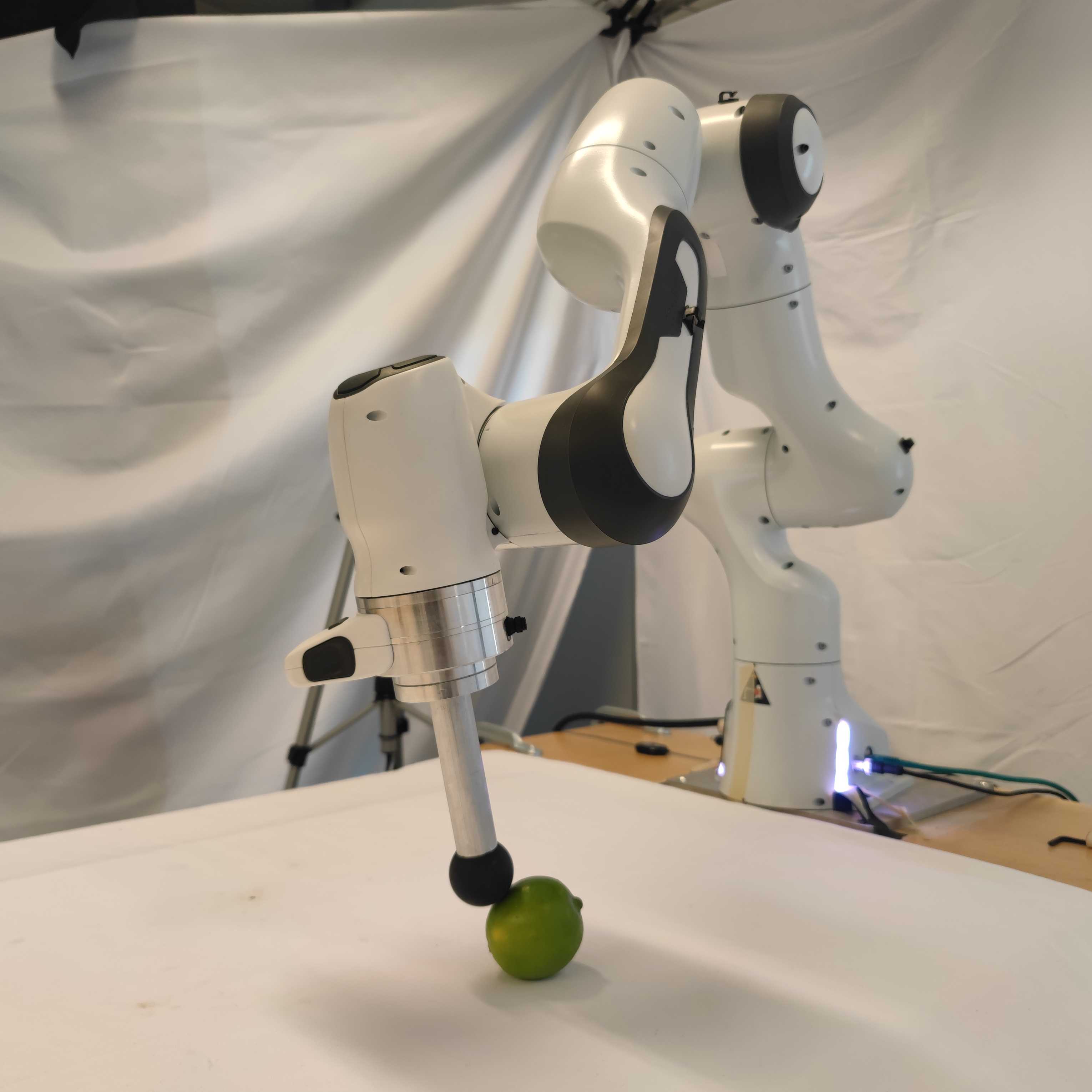
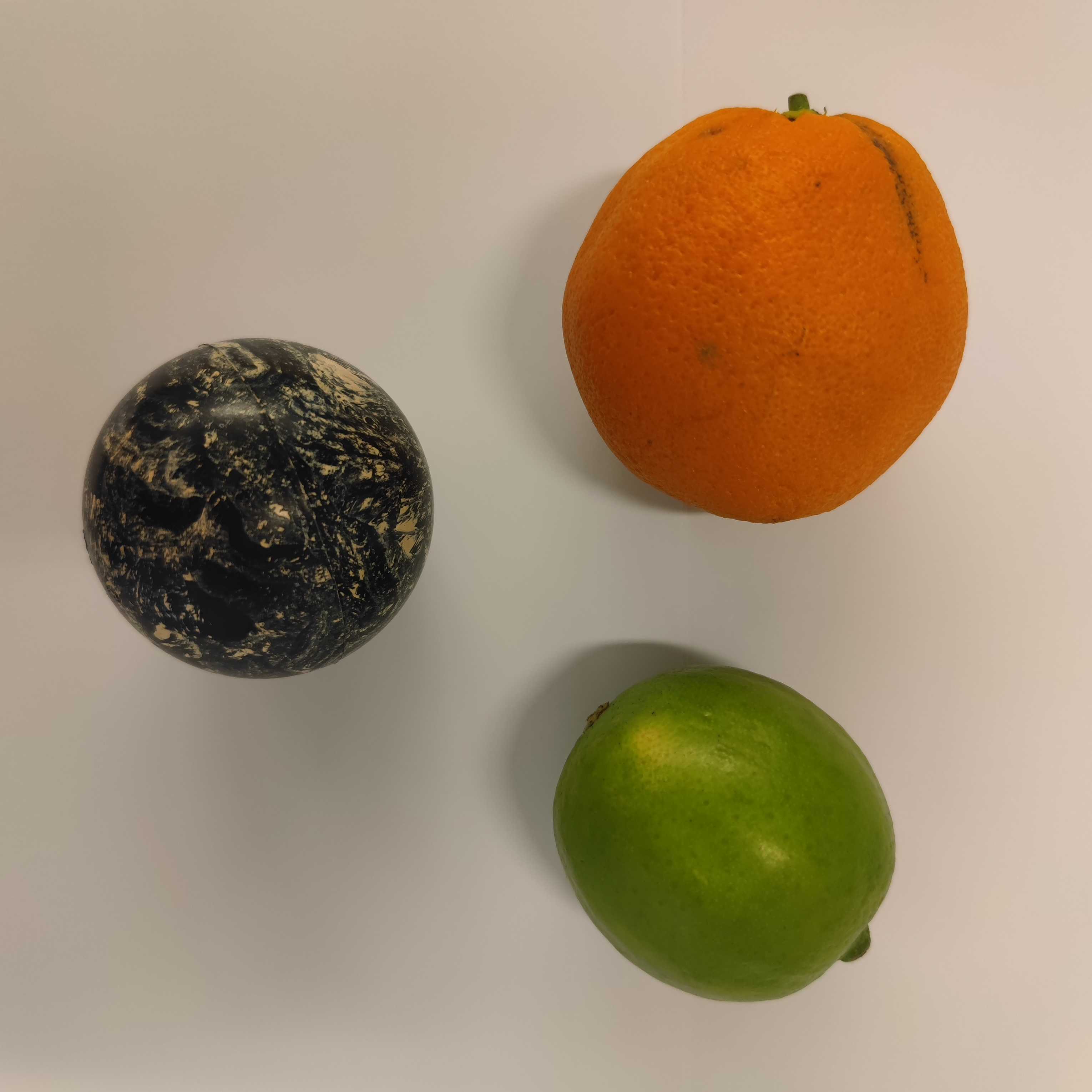
In this work, we present a novel adaptive contact-implicit MPC framework. It enables continuously adjusting the hybrid model from real-time in-stream data meanwhile the MPC controller uses the most recent model for high-quality control on multi-contact tasks. Compared to the existing work, we emphasize the two key contributions below.

(i) We present an adaptation law for multi-contact systems that continuously minimizes the gap between the prior model and reality by learning a hybrid residual model from in-stream data. It is inspired by our offline learning method [6] but unlike the previous work it focuses on online learning and utilizes physics-based prior models to speed up the process. Furthermore, the hybrid model adaption module is integrated into our fast multi-contact MPC controller [11] which allows real-time adaptive contact-implicit control on robots with on-the-fly performance improvement for contact-rich tasks.

(ii) We validate the proposed approach with two different hardware experiments, accomplishing challenging robot arm manipulation tasks. Our method adapts itself on-the-fly with an adaption rate around $20$ Hz and can consistently be employed to manipulate objects with uneven or irregular surface geometries. The findings also indicate that our approach can achieve success in tasks that purely model-based methods fail.

II Related Work

II-1 Learning Multi-Contact Dynamics Models

The hybrid nature of multi-contact dynamics poses challenges for gradient-based learning. One line of work, termed differentiable simulation, focuses on smoothing hybrid mode boundaries, although this can lead to approximation errors [12, 13, 14]. Recently, however, results have shown that conventional neural networks are limited in capturing the multi-modality and high-stiffness of multi-contact systems [15, 7, 16]. To address this, researchers [7, 6, 16] explicitly exploit the hybrid structure (complementarity formulation) of contact dynamics to develop learning algorithms, achieving state-of-the-art performance. In our adaptive contact-implicit MPC framework, the adaption module focuses on learning a hybrid residual model on top of prior dynamics, which is based on our previous work [6]. The benefits of [6] is that it simultaneously performs the mode partitioning and linear regression by proposing a novel training loss. The quadratic formulation in the loss enables fast updates using in-stream data, which can run up to $20$ Hz.

II-2 Fast Multi-Contact Model Predictive Control

To handle the combinatoric complexity of choosing hybrid contact modes, previous work [17, 18] use pre-defined sequence of modes to achieve real-time multi-contact control on legged locomotion [19] and manipulation [20]. To achieve contact-implicit control, the work [3] proposed to relax contact mode boundaries with smoothing approximation. Concurrently, our work [11] introduced an approach that preserves the hybrid structures while decoupling the combinatorial complexity from planning depth. However, rather than operating with an accessible ground-truth multi-contact model, we incorporate a hybrid model adaptation module into the MPC controller. This module operates continuously, updating the hybrid model with data collected from real-world interactions. Consequently, the MPC controller can consistently improve its performance for multi-contact tasks.

II-3 Task-Oriented Multi-Contact Modeling Learning

A relevant body of recent research is task-driven multi-contact model learning, which aims to find a model that can be used to (derive a policy and) accomplish given tasks. This line of work shares the same idea as deep model-based reinforcement learning [21], although the latter typically suffers from huge data demand. The most recent work focuses on learning a task-driven computationally affordable models, which have been shown requiring a small amount of data to successfully solve deleterious manipulation [4] and bipedal locomotion [5]. It is important to note that the above existing methods predominantly rely on an offline model learning. This means that the model undergoes episodic updates after accumulating a buffer of historical policy data. In contrast, the approach presented in this paper emphasizes continuous and online updates to the hybrid residual model. This innovative method facilitates real-time improvements in the multi-contact hybrid model, consequently improving performance during the deployment of the MPC policy. Additionally, this adaptation framework holds the potential to reduce data consumption when compared to offline model learning methodologies.

II-4 Adaptive MPC

The most relevant theme of this work is adaptive control, which focuses on control of uncertain systems through real-time model adaptation and learning [22] and has long been an ongoing research direction [23]. Researchers have developed robust (adaptive) MPC methods [24, 25, 26, 27], which are successfully applied to electric vehicles [28], climate control [29], quadrotors [30]. Similarly, there are multiple recent methods that perform adaptive MPC under unknown noise distributions [31] or incorporate components from adaptive control into learning-based MPC [32]. Also, the recent work [33] presents an adaptive MPC variant that automatically estimates control and model parameters by leveraging ideas from Bayesian optimization performing manipulation tasks. Unlike our approach which focuses on real-time adaptive MPC for systems that make and break contact, the authors focus on reaching tasks avoiding any contact interaction.

III Background

III-A Multi-Contact Dynamics

The multi-contact dynamics of a manipulator is

$$M(q)\dot{v}+C(q,v)=Bu+J(q)^{T}\lambda,$$ (1)

where $q$ is the generalized positions vector, $v$ is the generalized velocities, $\lambda$ represents the contact forces. The contact forces can be represented by the following complementarity equation:

$$0\leq\lambda\perp\psi(q,v,u,\lambda)\geq 0.$$ (2)

In this context, $\psi$ signifies the connection between the contact forces and the generalized positions, velocities, and inputs, as discussed in references [34, 35, 36]. We denote a multi-contact model with $\mathcal{M}_{c}=\{q,v,\dot{v},u,\lambda:\eqref{eq:manipulator_equation},\,\eqref{eq:manipulator_complementarity_constraints}\;\text{holds}\}$ and with a slight abuse of notation denote the dynamics $\dot{x}=\mathcal{M}_{c}(x,\lambda,u)$ with $x=\begin{bmatrix}q^{T},v^{T}\end{bmatrix}^{T}$.

III-B Linear Complementarity Problem

In this study, we employ linear complementarity problems (LCPs) as a means to depict contact forces [35, 36, 37].

Definition 1

Given a vector $q\in\mathbb{R}^{m}$, and a matrix ${F\in\mathbb{R}^{m\times m}}$, the $\text{LCP}(q,F)$ describes the following program:

$$\underset{}{\text{find}} \lambda\in\mathbb{R}^{m}$$

subject to $$y=F\lambda+q,$$

$$0\leq\lambda\perp y\geq 0.$$

III-C Linear Complementarity Systems

We employ linear complementarity systems (LCS) as localized models for multi-contact systems [38, 11, 39].

Definition 2

An LCS describes the trajectories $(x_{k})_{k\in\mathbb{N}_{0}}$ and $(\lambda_{k})_{k\in\mathbb{N}_{0}}$ for an input sequence $(u_{k})_{k\in\mathbb{N}_{0}}$ such that

$$x_{k+1}=Ax_{k}+Bu_{k}+D\lambda_{k}+d,$$ (3)

$$0\leq\lambda_{k}\perp Ex_{k}+F\lambda_{k}+Hu_{k}+c\geq 0,$$

for a given $x_{0}$ where $x_{k}\in\mathbb{R}^{n_{x}}$, $\lambda_{k}\in\mathbb{R}^{n_{\lambda}}$, $u_{k}\in\mathbb{R}^{n_{u}}$.

Given $x_{k}$ and $u_{k}$, you can determine the associated complementary variable $\lambda_{k}$ by solving the linear complementarity problem $\text{LCP}(Ex_{k}+Hu_{k}+c,F)$ (Definition 1). Moving forward, we describe the set of matrices in the LCS model (3) as $\theta=\{A,B,D,d,E,F,H,c\}$. If the elements depend on a given state-input pair ($x^{*},u^{*}$), we represent them as $A^{*}=A(x^{*},u^{*})$ and the set of such matrices is denoted as $\theta^{*}$. We denote the associated LCS model as $\mathcal{L}(\theta^{*})$. Similarly, with a slight abuse of notation, we denote the state-contact force pair an LCS generates as $(x_{k+1},\lambda_{k})=\mathcal{L}(x_{k},u_{k},\theta^{*})$.

III-D Consensus Complementarity Control (C3)

In our previous work, we presented a framework to solve model predictive control (MPC) problems with local hybrid models (details on how this non-convex problem can be solved at real-time rates can be found in the manuscript [11]):

$$\min_{x_{k},\lambda_{k},u_{k}} \sum_{k=0}^{N-1}(x_{k}^{T}Q_{k}x_{k}+u_{k}^{T}R_{k}u_{k})+x_{N}^{T}Q_{N}x_{N}$$ (4)

s.t. $$x_{k+1}=Ax_{k}+Bu_{k}+D\lambda_{k}+d,$$

$$0\leq\lambda_{k}\perp Ex_{k}+F\lambda_{k}+Hu_{k}+c\geq 0,$$

where $N$ is the planning horizon, $Q_{k},Q_{N}$ are positive semidefinite matrices and $R_{k}$ are positive definite matrices. Given an LCS model and an initial state, C3 returns an input, i.e. $u_{\text{C3}}=\text{C3}(x_{0},\mathcal{L}(\theta^{*}))$.

IV Problem Formulation

In this work, we are interested in solving the following MPC problem at real-time rates:

$$\min_{x_{k},\lambda_{k},u_{k}}\quad \sum_{k}g_{c}(x_{k},u_{k})$$ (5)

s.t. $$x_{k+1}=\mathcal{M}(x_{k},\lambda_{k},u_{k})$$

where $g_{c}$ is the cost, often quadratic and $\mathcal{M}$ is the discretization of $\mathcal{M}_{c}$ (for details [40]). As in MPC frameworks, one can utilize the first input after solving (5), denoted as $u_{0}(\mathcal{M})$ while repeatedly solving the problem in a receding horizon manner. Here, we operate under the assumption that we do not have access to the ground-truth multi-contact model $\mathcal{M}$ but possess an approximated version of it referred to as $\mathcal{M}^{\text{prior}}$.

In this setting, our aim is to collect data online and adaptively learn a residual $\mathcal{R}$ from scratch while simultaneously solving the following MPC problem, both at real-time rates:

$$\min_{x_{k},u_{k},\lambda_{k}}\quad \sum_{k}g_{c}(x_{k},u_{k})$$ (6)

s.t. $$x_{k+1}=\mathcal{M}^{\text{prior}}_{\mathcal{R}}(x_{k},\lambda_{k},u_{k})$$

where $\mathcal{M}^{\text{prior}}_{\mathcal{R}}$ represents our adaptive model. Because our adaptation acts jointly on the hybrid mode boundaries and their dynamics, $\mathcal{M}^{\text{prior}}_{\mathcal{R}}$ is not the result of summation of prior dynamics and residual as in classical residual learning frameworks, and will be described in Section VI. Our goal is that, over time, our adaptive model, $\mathcal{M}^{\text{prior}}_{\mathcal{R}}$ accurately captures the behavior of the true dynamics $\mathcal{M}$, and that $u_{0}(\mathcal{M}^{\text{prior}}_{\mathcal{R}})$ well-approximates $u_{0}(\mathcal{M})$ in (5). We highlight that we want to achieve both goals at real-time rates.

V Physics-Based LCS

This section describes a process of converting Anitescu’s approach for simulating contact dynamics [36] into an LCS approximation around a given state-input pair $(x^{*},u^{*})$. We choose Anitescu’s formulation over other approaches, such as the Stewart-Trinkle formulation [41], because it is a convex contact model (i.e. $F^{*}$ as in Section III-C is positive semi-definite for any $x^{*}$ and $u^{*}$) and our proposed learning algorithm (discussed in Section VI) relies on this assumption. Next, we describe our physics based model, $\mathcal{M}^{\text{prior}}$, which is a discrete-time approximation of (1), (2):

$$q_{k+1}=q_{k} +\Delta tv_{k+1},$$ (7)

$$v_{k+1}=v_{k} +M^{-1}\bigg{(}\Delta tBu_{k}-\Delta tC(q_{k},v_{k})+J_{c}(q_{k})^{T}\lambda_{k}\bigg{)},$$

with the complementarity constraints:

$$0\leq\lambda_{k}\perp\frac{E_{t}^{T}}{\Delta t}\bigg{(}\phi+J_{n}(q_{k})(q_{k+1}-q_{k})\bigg{)}+\mu J_{t}(q_{k})v_{k+1}\geq 0.$$ (8)

Here $\phi$ represents the distance between rigid body pairs, $J_{n}$, $J_{t}$ are contact Jacobians for normal and tangential directions, the contact Jacobian is defined as $J_{c}=E_{t}^{T}J_{n}+\mu J_{t}$, $\mu$ represents the coefficient of friction and $E_{t}=\mathbf{blkdiag}(e,\ldots,e)$ with $e=[1,\ldots,1]\in\mathbb{R}^{1\times n_{e}}$ (where $n_{e}$ represents the number of edges of the polyhedral approximation of the friction cone).

Given state $(x^{*})^{T}=[(q^{*})^{T},(v^{*})^{T}]$ and input $u^{*}$, we can approximate (7) as:

$$q_{k+1}=q_{k}+\Delta tv_{k+1},$$ (9)

$$v_{k+1}=v_{k}+\Delta tJ_{f}\begin{bmatrix}q_{k}^{T}&v_{k}^{T}&u_{k}^{T}\end{bmatrix}^{T}+D\lambda_{k}+d_{v},$$

where $J_{f}=J_{f}(q^{*},v^{*},u^{*})$ is the Jacobian of $f(q,v,u)=M^{-1}(q)Bu-M^{-1}(q)C(q,v)$ evaluated at $(q^{*},v^{*},u^{*})$, $d_{v}=f(q^{*},v^{*},u^{*})-J_{f}\begin{bmatrix}(q^{*})^{T}&(v^{*})^{T}&(u^{*})^{T}\end{bmatrix}^{T}$ is a constant vector and $D=M^{-1}(q^{*})J_{c}(q^{*})^{T}$. Similarly the equation (8) can be approximated as:

$$0\leq\lambda_{k}\perp\frac{1}{\Delta t}E_{t}^{T}\bigg{(}\phi(q^{*}) +J_{n}(q^{*})q_{k}-J_{n}(q^{*})q^{*}\bigg{)}$$ (10)

$$+J_{c}(q^{*})v_{k+1}+\epsilon_{c}\lambda_{k}\geq 0.$$

We note that because simulation considers single-step predictions, and MPC requires multi-step predictions, (9)-(10) differs slightly from the LCS presented in previous work [36]. These equations can be written in the LCS format (3) and represented as $\mathcal{L}(\theta^{*})$. We have also introduced a regularizing term $\epsilon_{c}\lambda_{k}$ in (10) to ensure that $F^{*}$ is positive definite as Anitescu’s formulation produces a positive semi-definite $F^{*}$.

VI Adaptive MPC with Residual Learning

Algorithm 1

0:  $c_{r},\mathcal{B},\epsilon,\gamma,\xi$

1:  Compute $\theta^{*}$ for each data point and construct $\mathcal{B}^{A}$

2:  Compute the gradient $\nabla_{c_{r}}L_{\epsilon}(\mathcal{B}^{A},c_{r})$

3:  Update the residual $c_{r}$ via Adam [42]

4:  return  $c_{r}$ (updated residual parameter)

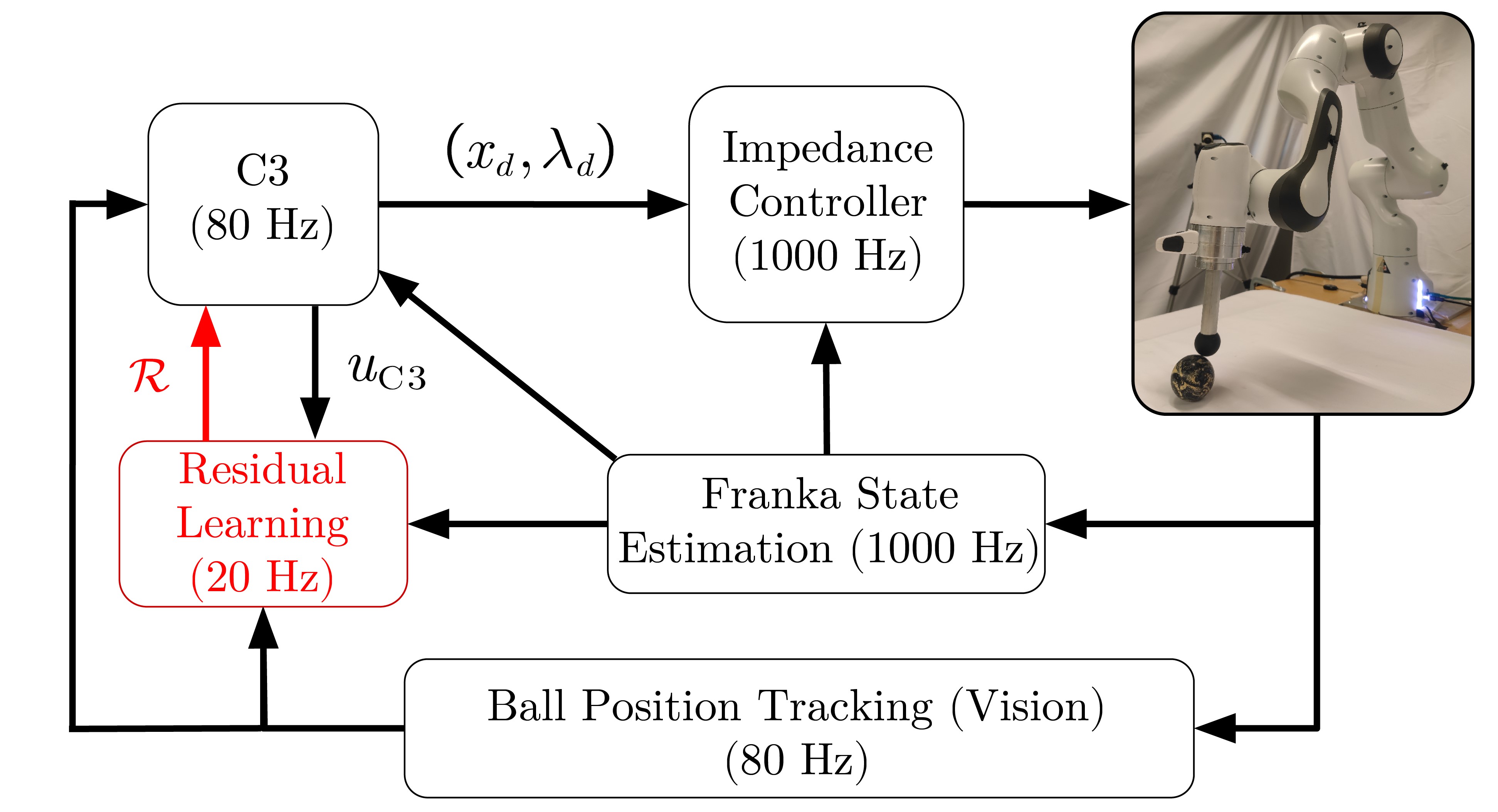
In this section, we describe our adaptive MPC framework shown in Figure 2. First, we describe the residual learning module (shown in red) in detail. Then we give details about the interaction of the residual learning module with C3.

Standard residual learning [43] focuses on models:

$$x_{k+1}=\mathcal{M}^{\text{prior}}(x_{k},u_{k})+\mathcal{R}_{\text{traditional}}(x_{k},u_{k}),$$ (11)

where the prior model and the learned residual are combined in an additive manner. If we consider our physics based model, $\mathcal{M}^{\text{prior}}$, to be an LCS (as in Section V), (11) is equivalent to:

$$x_{k+1} =A^{*}x_{k}+B^{*}u_{k}+D^{*}\lambda_{k}+d^{*}+\mathcal{R}_{\text{traditional}}(x_{k},u_{k}),$$ (12)

$$0\leq\lambda_{k}\perp E^{*}x_{k}+F^{*}\lambda_{k}+H^{*}u_{k}+c^{*}\geq 0,$$

and one can use state-of-the-art residual learning frameworks [44, 45] to learn $\mathcal{R}_{\text{traditional}}$. This form of adaptation is well studied, and not the focus of this paper. Furthermore, because (12) does not adapt the hybrid structure encoded in the complementarity constraints, it is doomed to be data inefficient and will struggle to adapt [15, 16]. Unlike in prior methods, our focus is on learning both the hybrid boundary and the contact dynamics:

$$x_{k+1}=A^{*}x_{k}+B^{*}u_{k}+D^{*}\lambda_{k}+d^{*},$$ (13)

$$0\leq\lambda_{k} \perp E^{*}x_{k}+F^{*}\lambda_{k}+H^{*}u_{k}+c^{*}+\mathcal{R}(x_{k},u_{k},\lambda_{k})\geq 0,$$

where $\mathcal{R}$ represents the model error in contact equation, e.g. (10) and this effect implicitly appears in the dynamics equation. We will focus on learning a residual that is of the form $c_{r}\in\mathbb{R}^{n_{\lambda}}$ as we have observed high performance in our experiments with this choice, but our framework is easily adaptable to the more general setting. This residual, denoted as $c_{r}$, possesses the ability to capture inaccuracies such as those in normal distance, tangential friction directions and coefficients of friction. Hence, we consider:

$$x_{k+1}=A^{*}x_{k}+B^{*}u_{k}+D^{*}\lambda_{k}+d^{*},$$ (14)

$$0\leq\lambda_{k} \perp E^{*}x_{k}+F^{*}\lambda_{k}+H^{*}u_{k}+c^{*}+c_{r}\geq 0,$$

where we learn the vector $c_{r}$ adaptively at real-time rates to compensate the error. We note that, as in traditional residual learning, our learned residual term $c_{r}$ might be time-varying, and thus also capture state-dependent variations in the complementarity constraints. Equation (14) consists of physics based model parameters $\theta^{*}$, derived (via Anitescu formulation) from our prior knowledge of the system and also the residual vector $c_{r}$ that is learned by collecting data during the experiment. We denote (14) as $\mathcal{L}(\theta^{*},c_{r})$ that combines the prior model $\mathcal{M}^{\text{prior}}$ with the learned residual $\mathcal{R}$.

Figure 2: Key elements of the adaptive MPC framework. Given proprioception and visual data, our method learns a residual multi-contact model at $20$ Hz, which we use for real-time control.

Figure 3: A “contact event” refers to a situation where actual physical contact is occurring, while “contact prediction” pertains to instances where the model anticipates contact, potentially inaccurately. Our method can produce meaningful gradients, even when there is no actual contact event (yellow region). The only scenario in which a zero gradient is produced is when the model and data both agree that there is no contact (white region).

Once an experiment starts, we collect data of the form $\mathcal{B}=\{x_{k+1},x_{k},u_{k}\}_{k=n_{ct}}^{n_{ct}+n_{b}}$ into our buffer where $n_{ct}$ represents the current time-step and $n_{b}$ is the number of data points stored. For each $(x_{k},u_{k})$, we also calculate the corresponding LCS matrices $\theta_{k}^{*}$ (consists of $A^{*}_{k},B^{*}_{k},\ldots$) via the method described in Section V and define the buffer appended with those matrices as $\mathcal{B}^{A}=\{x_{k+1},x_{k},u_{k},\theta_{k}^{*}\}_{k=n_{ct}}^{n_{ct}+n_{b}}$. Next, we introduce a variant of the implicit loss function that was defined in [6]:

$$L_{\epsilon}(\mathcal{B}^{A},c_{r})=\sum_{k=n_{ct}}^{n_{ct}+n_{b}}l_{\epsilon}(x_{k+1},x_{k},u_{k},\theta^{*}_{k},c_{r}),$$

where the function $l_{\epsilon}(x_{k+1},x_{k},u_{k},\theta^{*}_{k},c_{r})$ is defined as

$$l_{\epsilon}(\cdot) =\min_{\lambda_{k}\geq 0,\eta_{k}\geq 0}\frac{1}{2}(D^{*}_{k}\lambda_{k}+z)^{T}Q_{d}(D^{*}_{k}\lambda_{k}+z)$$

$$+\frac{1}{\epsilon}\big{(}\lambda_{k}^{T}\eta_{k}+\frac{1}{2\gamma}\big{|}\big{|}q+F^{*}_{k}\lambda_{k}+c_{r}-\eta_{k}\big{|}\big{|}^{2}\big{)},$$

where $z=A_{k}^{*}x_{k}+B_{k}^{*}u_{k}+d_{k}^{*}-x_{k+1}$ and $q=E^{*}_{k}x_{k}+H^{*}_{k}u_{k}+c^{*}_{k}$. Here, $\gamma$ is a constant such that $0<\gamma<\sigma_{\min}\big{(}(F_{k}^{*})^{T}+F_{k}^{*}\big{)}$ for all $k$ where $\sigma_{\min}(\cdot)$ denotes the smallest singular value. It is important to note that based on our specific formulation using Anitescu’s method, all $F_{k}^{*}$ are positive definite and we can always find a $\gamma$ that satisfies the given equality. Similarly, $\epsilon$ is a constant such that $\epsilon>0$. Under these conditions, we can calculate the gradient of the loss function with respect to the residual parameter $c_{r}$, i.e. $\nabla_{c_{r}}L_{\epsilon}(\cdot)$ following our previous work [6]. This approach requires solving a single quadratic program per data point in the batch (hence is relatively fast). After gradient calculations, residual parameters are updated with a simple gradient step (via learning rate $\xi>0$). Following this discussion, Algorithm 1 summarizes how the proposed learning method works.

Both our residual learning module and C3 run at real-time rates (Figure 2). The MPC algorithm uses the latest residual value $c_{r}$, as well as the current state $x^{*}$ and computes the optimal input $u_{\text{C3}}=\text{C3}(x^{*},\mathcal{L}(\theta^{*},c_{r}))$. Then, the desired next state-contact force pair is computed as $(x_{d},\lambda_{d})=\mathcal{L}(x^{*},u_{\text{C3}},\theta^{*},c_{r})$. An impedance controller is used to track the desired values [46, 47].

VII Examples

VII-A Synthetic Example: Cart-pole with Soft Walls

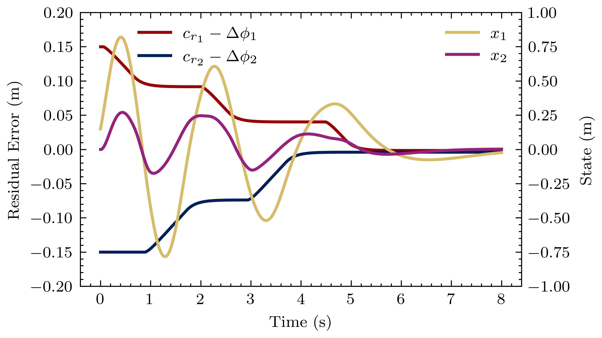
We consider a classical cart-pole underactuated system which has been augmented with two soft walls (Figure 3). The pole can contact these walls, requiring contact-aware control to stabilize the system (for further details, see [38]):

$$x_{k+1}=Ax_{k}+Bu_{k}+D\lambda_{k}+d,$$

$$0\leq\lambda_{k}\perp Ex_{k}+F\lambda_{k}+c\geq 0,$$

where we have perfect knowledge of the parameters except for $c$. We write $c=\hat{c}+\Delta\phi$, where $\hat{c}$ is our initial guess of the parameter. For the purposes of illustration, we begin with an initial error of $\Delta\phi=[-.15,.15]$. Notice that the model error that is related to each contact ($\lambda_{k}$) has a different sign. Our deliberate choice of this setup was made to create a range of scenarios, allowing the contact model to predict both situations: contact and no contact, as well as the presence or absence of actual contact events during those situations. In Figure 3, it can be seen that our method successfully returns useful gradient information in all of those scenarios. We highlight that our approach is capable of adapting even when there is no actual contact events (Figure 3). We also show that our framework successfully stabilizes the system as well as learning the true residual values (Figure 4).

Figure 4: Stabilization of the cart-pole system and convergence of residual.

VII-B Hardware Experiment: Adaptive Trajectory Tracking

Here, we show that our real-time adaptive MPC framework can reliably be used for multi-contact manipulation tasks that require high-speed reasoning about contact events. Our goal is to roll a rigid ball along a circular trajectory using a Franka Emika Panda Arm (Figure 1). We perform vision-based estimation for the ball using Hough transform [48] and utilize an impedance controller [47, 46] to track high-level commands that our adaptive MPC produces (Figure 2). For adaptive MPC, we simplify the arm as a point contact. For full details please check the manuscript [11].

In previous work, careful manual identification of model parameters was required to achieve success [11]. Here, via our adaptive MPC approach, we do not need to assume access to an accurate model. For this experiment, the actual radius of the ball ($\mathcal{M}$) is $5$ mm smaller than our parameter estimation ($\mathcal{M}^{\text{prior}}$). The state estimation for the ball is noisy (vision-based, $80$ Hz) and we do not have accurate estimation of many model parameters such as coefficient of friction. As a result, MPC with this incorrect model fails to interact with the ball, and therefore fails to accomplish the task. Due to the stiff, hybrid nature of contact dynamics, we have found MPC to be highly sensitive to modeling errors that effect the contact/no-contact transition.

Figure 5: Rolling a rigid ball and fruits (left: ball, middle: orange, right: lime) starting with an inaccurate model.

Figure 6: Hardware Experiment: Residual evolution of end-effector and ball contact pair, and loss curve of the learning process. The full experiment lasts for $315$ s. We highlight the adaptation process until loss and residual converge.

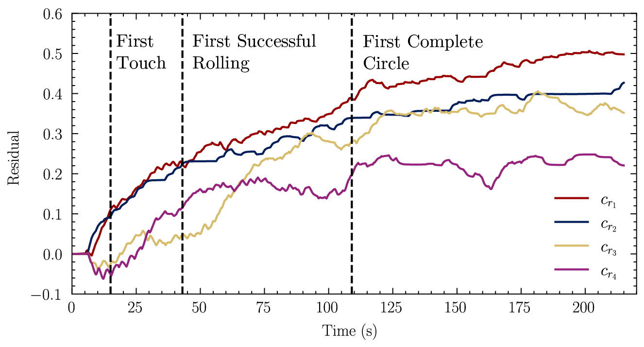
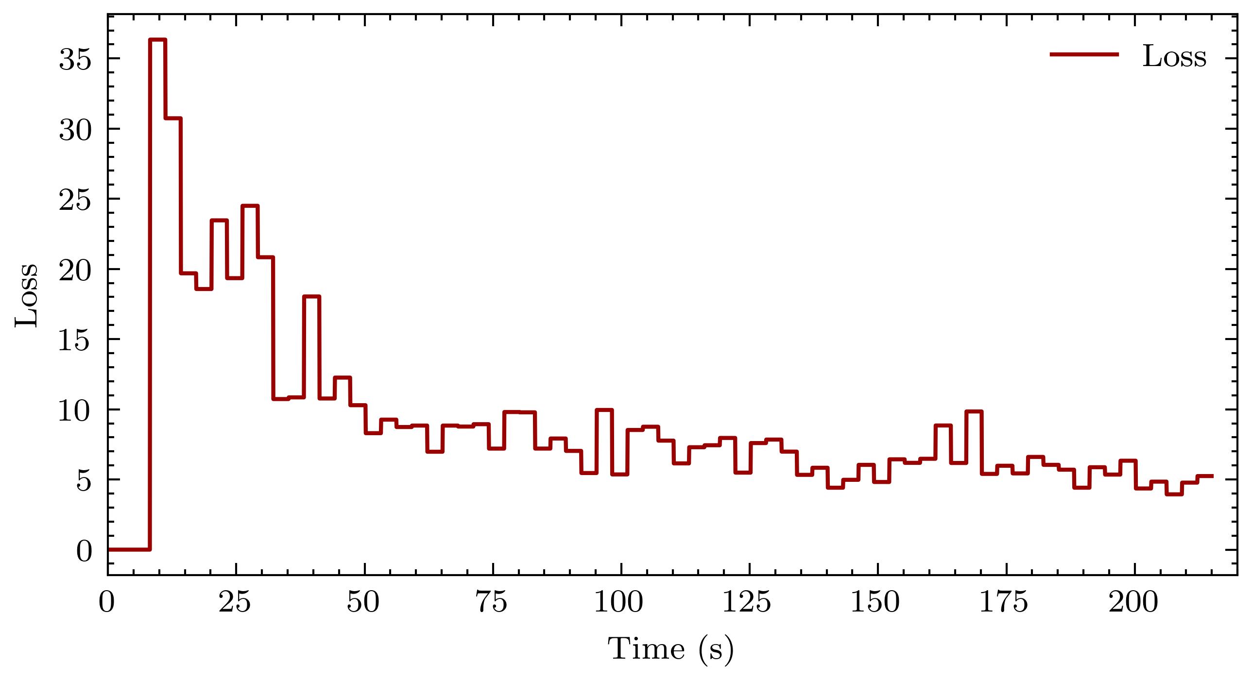
Even though the purely model-based approach fails, our adaptive MPC framework successfully accomplishes the task. The residual learning module (Algorithm 1, $20$ Hz), in combination with the C3 module ($80$ Hz), identifies the discrepancy at real-time rates. In the supplementary video, it can be observed that at the beginning the end-effector misses the ball due to inaccurate radius estimation. The C3 module then tries, and fails, to initiate contact. As motivated earlier, this discrepancy creates a non-zero gradient and therefore the residual values that correspond to end-effector ball contact pair gradually increase (shown in Figure 6).

In the end, with the learned residual compensating for the inaccurate model, our approach successfully rolls the ball for $4$ successive circles. Figure 6 shows the loss, $\mathcal{L}_{\epsilon}$, as well as the residual, $c_{r}$, for this experiment. The residual for the end-effector and ball contact shows convergence as the rolling proceeds and the loss curve shows a decreasing trend, proving the effectiveness of our method. We note that in this experiment, the LCP violation rate is $\epsilon=10^{-7}$, the terms in $Q_{d}$ related to balls translational velocity are set to $10^{5}$ (others are set to zero), learning rate is $\xi=10^{-3}$, stiffness parameter is $\gamma=10^{-2}$ and we have a batch data size of $n_{b}=10$. We demonstrate the trajectories of the ball with respect to the desired path in Figure 5.

VII-C Hardware Experiment: Objects of Non-smooth Surface

We repeat the previous hardware experiment (Section VII-B) with slightly deformable objects that have non-smooth surface geometries (Figure 1). We do not have accurate initial estimates of the geometry as our estimate of a fruit’s geometry is simply a sphere. For each experiment experiments, we assign an approximate radius for the given fruit and set the sphere radius in our prior model, $\mathcal{M}^{\text{prior}}$, accordingly.

Due to the bulges and dents on the fruit’s surface, initiating rolling can be hard since the fruit can roll back even after a push in the correct direction. MPC without adaptation gets stuck in the beginning and fails to even initiate rolling. In contrast, our method quickly adapts and starts making stronger pushes to initiate rolling (as shown in the supplementary video). In $90$% of the $20$ experiments, our method successfully initiated rolling and started tracking the circular path, while MPC without adaptation was never successful ($0$%).

Fruits tend to produce unpredictable motions at times due to its non-smooth surface geometry, but our method can adapt and accomplish the task. Our approach has managed to track at least one circle for $70$% of the trials with orange and $50$% of trials with lime ($20$ experiments for each case). In Figure 5, we report the long-term tracking (4 successive circles) performance of our method with multiple different fruits. The videos of experiments are in the supplementary material.

VIII Conclusion

We presented an adaptive model predictive control framework for multi-contact systems. The approach uses online residual updates and adaptively compensates model errors and uncertainties at real-time rates. The effectiveness of the method has been shown on multiple hardware experiments, including high-dimensional manipulation problems that include objects with non-smooth surface geometries (fruits).

We have further shown examples where pure model-based control fails but our adaptive strategy leads to success. We have also demonstrated that our learning module is capable of learning the contact model accurately even without actual contact interactions. Also, our parameter estimation can converge to the true parameter values at real-time rates.

We are interested in exploring a wider range of residual models in the future. For example, we might extend our results to include state-dependent terms, or simultaneously learn the non-contact and contact residuals. Integrating our framework with tactile sensors is also an interesting future direction which could speed up our learning process as well as increase the performance of the low-level controller [38].

References

- [1] Y. Tassa, T. Erez, and E. Todorov, “Synthesis and Stabilization of Complex Behaviors Through Online Trajectory Optimization,” in 2012 IEEE/RSJ International Conference on Intelligent Robots and Systems, pp. 4906–4913, IEEE, 2012.
- [2] A. Aydinoglu, V. M. Preciado, and M. Posa, “Contact-Aware Controller Design for Complementarity Systems,” arXiv preprint arXiv:1909.11221, 2019.
- [3] S. L. Cleac’h, T. Howell, M. Schwager, and Z. Manchester, “Fast contact-implicit model-predictive control,” arXiv preprint arXiv:2107.05616, 2021.
- [4] W. Jin and M. Posa, “Task-driven hybrid model reduction for dexterous manipulation,” arXiv preprint arXiv:2211.16657, 2022.
- [5] Y.-M. Chen and M. Posa, “Optimal reduced-order modeling of bipedal locomotion,” in 2020 IEEE International Conference on Robotics and Automation (ICRA), pp. 8753–8760, IEEE, 2020.
- [6] W. Jin, A. Aydinoglu, M. Halm, and M. Posa, “Learning linear complementarity systems,” in Learning for Dynamics and Control Conference, pp. 1137–1149, PMLR, 2022.
- [7] S. Pfrommer, M. Halm, and M. Posa, “Contactnets: Learning discontinuous contact dynamics with smooth, implicit representations,” in Conference on Robot Learning, pp. 2279–2291, PMLR, 2021.
- [8] H. Qi, A. Kumar, R. Calandra, Y. Ma, and J. Malik, “In-hand object rotation via rapid motor adaptation,” in Conference on Robot Learning, pp. 1722–1732, PMLR, 2023.
- [9] A. Kumar, Z. Fu, D. Pathak, and J. Malik, “Rma: Rapid motor adaptation for legged robots,” arXiv preprint arXiv:2107.04034, 2021.
- [10] S. Sastry, M. Bodson, and J. F. Bartram, “Adaptive control: stability, convergence, and robustness,” 1990.
- [11] A. Aydinoglu, A. Wei, and M. Posa, “Consensus complementarity control for multi-contact mpc,” arXiv preprint arXiv:2304.11259, 2023.
- [12] M. Geilinger, D. Hahn, J. Zehnder, M. Bächer, B. Thomaszewski, and S. Coros, “Add: Analytically differentiable dynamics for multi-body systems with frictional contact,” ACM Transactions on Graphics (TOG), vol. 39, no. 6, pp. 1–15, 2020.
- [13] E. Heiden, D. Millard, E. Coumans, and G. S. Sukhatme, “Augmenting differentiable simulators with neural networks to close the sim2real gap,” arXiv preprint arXiv:2007.06045, 2020.
- [14] T. A. Howell, S. L. Cleac’h, J. Brüdigam, J. Z. Kolter, M. Schwager, and Z. Manchester, “Dojo: A differentiable physics engine for robotics,” arXiv preprint arXiv:2203.00806, 2022.
- [15] M. Parmar, M. Halm, and M. Posa, “Fundamental challenges in deep learning for stiff contact dynamics,” in 2021 IEEE/RSJ International Conference on Intelligent Robots and Systems (IROS), pp. 5181–5188, IEEE, 2021.
- [16] B. Bianchini, M. Halm, N. Matni, and M. Posa, “Generalization bounded implicit learning of nearly discontinuous functions,” in Learning for Dynamics and Control Conference, pp. 1112–1124, PMLR, 2022.
- [17] J.-P. Sleiman, F. Farshidian, M. V. Minniti, and M. Hutter, “A unified mpc framework for whole-body dynamic locomotion and manipulation,” IEEE Robotics and Automation Letters, vol. 6, no. 3, pp. 4688–4695, 2021.
- [18] C. Mastalli, R. Budhiraja, W. Merkt, G. Saurel, B. Hammoud, M. Naveau, J. Carpentier, L. Righetti, S. Vijayakumar, and N. Mansard, “Crocoddyl: An efficient and versatile framework for multi-contact optimal control,” in 2020 IEEE International Conference on Robotics and Automation (ICRA), pp. 2536–2542, IEEE, 2020.
- [19] A. W. Winkler, C. D. Bellicoso, M. Hutter, and J. Buchli, “Gait and trajectory optimization for legged systems through phase-based end-effector parameterization,” IEEE Robotics and Automation Letters, vol. 3, no. 3, pp. 1560–1567, 2018.
- [20] F. R. Hogan and A. Rodriguez, “Reactive planar non-prehensile manipulation with hybrid model predictive control,” The International Journal of Robotics Research, vol. 39, no. 7, pp. 755–773, 2020.
- [21] A. Nagabandi, K. Konolige, S. Levine, and V. Kumar, “Deep dynamics models for learning dexterous manipulation,” in Conference on Robot Learning, pp. 1101–1112, PMLR, 2020.
- [22] A. M. Annaswamy and A. L. Fradkov, “A historical perspective of adaptive control and learning,” Annual Reviews in Control, vol. 52, pp. 18–41, 2021.
- [23] A. Becker, P. Kumar, and C.-Z. Wei, “Adaptive control with the stochastic approximation algorithm: Geometry and convergence,” IEEE Transactions on Automatic Control, vol. 30, no. 4, pp. 330–338, 1985.
- [24] M. Tanaskovic, L. Fagiano, R. Smith, and M. Morari, “Adaptive receding horizon control for constrained mimo systems,” Automatica, vol. 50, no. 12, pp. 3019–3029, 2014.
- [25] H. Fukushima, T.-H. Kim, and T. Sugie, “Adaptive model predictive control for a class of constrained linear systems based on the comparison model,” Automatica, vol. 43, no. 2, pp. 301–308, 2007.
- [26] A. Weiss and S. Di Cairano, “Robust dual control mpc with guaranteed constraint satisfaction,” in 53rd IEEE Conference on Decision and Control, pp. 6713–6718, IEEE, 2014.
- [27] V. R. Desaraju, A. Spitzer, and N. Michael, “Experience-driven predictive control with robust constraint satisfaction under time-varying state uncertainty.,” in Robotics: Science and Systems, 2017.
- [28] S. Wang, K. Pei, J. Whitehouse, J. Yang, and S. Jana, “Efficient formal safety analysis of neural networks,” in Advances in Neural Information Processing Systems, pp. 6367–6377, 2018.
- [29] Y. Ma, S. Vichik, and F. Borrelli, “Fast stochastic mpc with optimal risk allocation applied to building control systems,” in 2012 IEEE 51st IEEE Conference on Decision and Control (CDC), pp. 7559–7564, IEEE, 2012.
- [30] K. Pereida and A. P. Schoellig, “Adaptive model predictive control for high-accuracy trajectory tracking in changing conditions,” in 2018 IEEE/RSJ International Conference on Intelligent Robots and Systems (IROS), pp. 7831–7837, IEEE, 2018.
- [31] C. Stamouli, A. Tsiamis, M. Morari, and G. J. Pappas, “Adaptive stochastic mpc under unknown noise distribution,” in Learning for Dynamics and Control Conference, pp. 596–607, PMLR, 2022.
- [32] K. Y. Chee, T. C. Silva, M. A. Hsieh, and G. J. Pappas, “Enhancing sample efficiency and uncertainty compensation in learning-based model predictive control for aerial robots,” arXiv preprint arXiv:2308.00570, 2023.
- [33] R. Guzman, R. Oliveira, and F. Ramos, “Adaptive model predictive control by learning classifiers,” in Learning for Dynamics and Control Conference, pp. 480–491, PMLR, 2022.
- [34] B. Brogliato, Nonsmooth Mechanics: Models, Dynamics and Control. Springer, 2016.
- [35] D. Stewart and J. C. Trinkle, “An Implicit Time-stepping Scheme for Rigid Body Dynamics with Coulomb Friction,” in Proceedings 2000 ICRA. Millennium Conference. IEEE International Conference on Robotics and Automation. Symposia Proceedings (Cat. No. 00CH37065), vol. 1, pp. 162–169, IEEE, 2000.
- [36] M. Anitescu, “Optimization-based simulation of nonsmooth rigid multibody dynamics,” Mathematical Programming, vol. 105, pp. 113–143, 2006.
- [37] R. W. Cottle, J.-S. Pang, and R. E. Stone, The Linear Complementarity Problem. SIAM, 2009.
- [38] A. Aydinoglu, P. Sieg, V. M. Preciado, and M. Posa, “Stabilization of complementarity systems via contact-aware controllers,” IEEE Transactions on Robotics, vol. 38, no. 3, pp. 1735–1754, 2021.
- [39] W. Heemels, J. M. Schumacher, and S. Weiland, “Linear Complementarity Systems,” SIAM Journal on Applied Mathematics, vol. 60, no. 4, pp. 1234–1269, 2000.
- [40] M. Posa, C. Cantu, and R. Tedrake, “A Direct Method for Trajectory Optimization of Rigid Bodies Through Contact,” The International Journal of Robotics Research, vol. 33, no. 1, pp. 69–81, 2014.
- [41] D. E. Stewart, “Rigid-body Dynamics with Friction and Impact,” SIAM review, vol. 42, no. 1, pp. 3–39, 2000.
- [42] D. P. Kingma and J. Ba, “Adam: A method for stochastic optimization,” arXiv preprint arXiv:1412.6980, 2014.
- [43] T. Koller, F. Berkenkamp, M. Turchetta, and A. Krause, “Learning-based model predictive control for safe exploration,” in 2018 IEEE conference on decision and control (CDC), pp. 6059–6066, IEEE, 2018.
- [44] G. Kulathunga, H. Hamed, and A. Klimchik, “Residual dynamics learning for trajectory tracking for multi-rotor aerial vehicles,” arXiv preprint arXiv:2305.15791, 2023.
- [45] G. Torrente, E. Kaufmann, P. Föhn, and D. Scaramuzza, “Data-driven mpc for quadrotors,” IEEE Robotics and Automation Letters, vol. 6, no. 2, pp. 3769–3776, 2021.
- [46] O. Khatib, “A unified approach for motion and force control of robot manipulators: The operational space formulation,” IEEE Journal on Robotics and Automation, vol. 3, no. 1, pp. 43–53, 1987.
- [47] N. Hogan, “Impedance control: An approach to manipulation,” in 1984 American control conference, pp. 304–313, IEEE, 1984.
- [48] R. O. Duda and P. E. Hart, “Use of the hough transformation to detect lines and curves in pictures,” Communications of the ACM, vol. 15, no. 1, pp. 11–15, 1972.