On best-response algorithms for monotone Nash equilibrium problems with mixed-integer variables

Abstract

We characterize the convergence properties of traditional best-response (BR) algorithms in computing solutions to mixed-integer Nash equilibrium problems (MI-NEPs) that turn into a class of monotone Nash equilibrium problems (NEPs) once relaxed the integer restrictions. We show that the sequence produced by a Jacobi/Gauss-Seidel BR method always approaches a bounded region containing the entire solution set of the MI-NEP, whose tightness depends on the problem data, and it is related to the degree of strong monotonicity of the relaxed NEP. When the underlying algorithm is applied to the relaxed NEP, we establish data-dependent complexity results characterizing its convergence to the unique solution of the NEP. In addition, we derive one of the very few sufficient conditions for the existence of solutions to MI-NEPs. The theoretical results developed bring important practical advantages that are illustrated on a numerical instance of a smart building control application.

1 Introduction

In many real-world applications different decision makers frequently interact in a non-cooperative fashion to take optimal decisions that may depend on the opponents’ strategies. If these decisions have to be made simultaneously, every agent is rational and has complete information about the other agents’ optimization problems, then Nash equilibria can be considered as solutions of the resulting non-cooperative game. Theory and algorithms to solve Nash equilibrium problems (NEPs) have been widely investigated in the literature, but mostly considering continuous strategy spaces for the agents – see, e.g., FacchKanSu ; scutari2012monotone ; scutari2014real ; grammatico2017dynamic ; dreves2011solution ; dreves2020nonsingularity ; bigi2023approximate . Despite in many crucial situations it is rather natural to restrict some variables to exclusively assume integer values, relevant contributions along this direction appeared only very recently in the literature and, to the best of our knowledge, they can be summarized as follows.

• Enumerative techniques for general instances. A branch-and-prune method to compute the whole set of solutions in the integer case was proposed in the seminal work sagratella2016computing , which has successively been extended in sagratella2019generalized to solve mixed-integer Nash equilibrium problems (MI-NEPs) with linear coupling constraints. Very recently, the method has been further boosted to encompass non-linearities and non-convexities schwarze2023branch .

• Best-response algorithms for potential problems. In sagratella2017algorithms has been proved that Gauss-Seidel best-response (BR) algorithms always converge to (approximate) mixed-integer Nash equilibria (MI-NE) and there are no solutions that can not be computed in this way. More recently, fabiani2022proximal discussed how integer-compatible regularization functions enable for convergence either to an exact or approximate MI-NE.

• Best-response algorithms for 2-groups partitionable instances. This class of problems was defined in sagratella2016computing and arises in several economics and engineering applications, see e.g. sagratella2017computing ; passacantando2023finite . Jacobi-type BR algorithms can be effectively used to compute equilibria for these games.

Finally, we mention tailored solution algorithms for (potential) MI-NEPs proposed for specific engineering applications spanning from automated driving fabiani2018mixed ; fabiani2019multi and smart mobility cenedese2021highway to demand-side management cenedese2019charging .

So far, there are no works on MI-NEPs in which monotonicity of the relaxed, i.e., fully continuous, version associated has been explicitly used to study problem solvability and convergence of BR methods. This is a fundamental gap in the literature, as monotonicity is a key condition to prove many theoretical properties for continuous NEPs FacchPangBk . We thus concentrate on the class of continuous NEPs with contraction properties (see Assumption 1) introduced in scutari2012monotone , which we extend to a mixed-integer setting by requiring additional conditions on the distance between continuous and mixed-integer BRs (see Assumption 2), and show that the resulting MI-NEPs enjoy several interesting properties. Our main contributions can hence be listed as follows.

• Focusing on a Jacobi/Gauss-Seidel BR method (Algorithm 1), we show that the sequence produced always approaches a bounded region containing the entire solution set of the MI-NEP– see Theorems 3.1, 3.4. The smaller the constants in Assumptions 1 and 2, the smaller the area of this region. This brings several numerical advantages, as discussed in Section 5.

• We establish a relation between the contraction property defined in Assumption 1 and the degree of (strong) monotonicity of the problem – see Section 4.1. Specifically, we propose different ways to obtain Assumption 1 by suitably perturbing any strongly monotone problem, see Proposition 3.

  In addition, we consider several Nash problem structures to obtain different constant values satisfying Assumption 2 – Section 4.2. As emphasized in those sections, the class of problems considered in this paper is thus wide and can be employed to model many real-world applications.

• We consider the Jacobi-type continuous BR method (Algorithm 2) to confirm convergence to the unique solution of the continuous NEP relaxation of the original MI-NEP (as stated in scutari2012monotone ). In addition, i) we provide some complexity results – see Theorem 3.2, and ii) show that Algorithm 2 has similar convergence properties as Algorithm 1 for the MI-NEP– see Theorem 3.3, also discussing the related numerical advantages in Section 5.

• We establish one of the very few sufficient conditions for the existence of solutions to MI-NEPs– see Proposition 1. Our conditions depend only on the constants defined in Assumptions 1 and 2, and on the unique solution of the continuous NEP relaxation of the original MI-NEP. Therefore, they are general and can be used to define solvable problems. In addition, if these conditions hold true, then there is a unique MI-NE and it can be computed through Algorithm 1.

• In Section 5 we finally corroborate our theoretical findings on a novel application involving the smart control of a building in which a number of residential units, endowed with some storing capacity, is interested in designing an optimal schedule to switch on/off high power domestic appliances over a prescribed time window to make the energy supply of the entire building smart and efficient.

2 Problem definition and main assumptions

Consider a NEP with $N$ players, indexed by the set $\mathcal{I}\triangleq\{1,\ldots,N\}$, and let $\nu\in\mathcal{I}$ be a generic player of the game. We denote by $x^{\nu}\in\mathbb{R}^{n_{\nu}}$ the vector representing the private strategies of the $\nu$-th player, and by ${\bf x}^{-\nu}\triangleq(x^{\nu^{\prime}})_{\nu^{\prime}\in\mathcal{I}\setminus\{\nu\}}$ the vector of all the other players strategies. We write $\mathbb{R}^{n}\ni{\bf x}\triangleq(x^{\nu},{\bf x}^{-\nu})$, where $n\triangleq\sum_{\nu\in\mathcal{I}}n_{\nu}$, to indicate the collective vector of strategies. Any player $\nu$ has to solve an optimization problem that is parametric with respect to (w.r.t.) the other players variables, and the resulting NEP reads as:

$$\forall\nu\in\mathcal{I}:\left\{\begin{aligned} &\underset{x^{\nu}}{\min}&&\theta_{\nu}(x^{\nu},{\bf x}^{-\nu})\\ &\textrm{ s.t. }&&x^{\nu}\in\Omega_{\nu}\triangleq\{x^{\nu}\in X_{\nu}\mid x^{\nu}_{j}\in{\mathbb{Z}},\,j=1,\ldots,i_{\nu}\},\end{aligned}\right.$$ (1)

where the cost functions $\theta_{\nu}\,:\,{\mathbb{R}}^{n}\,\rightarrow\,{\mathbb{R}}$ are continuously differentiable and convex w.r.t. $x^{\nu}$, $X_{\nu}\subseteq{\mathbb{R}}^{n_{\nu}}$ are (possibly unbounded) convex and closed sets, $i_{\nu}\leq n_{\nu}$ are nonnegative integers, and the feasible regions $\Omega_{\nu}$ are nonempty. We will assume throughout that any optimization problem $\nu$ in (1) always admits a solution for every given ${\bf x}^{-\nu}$. We remark that if $i_{\nu}=0$ for all $\nu$, i.e. the component-wise integer restrictions imposed through $x^{\nu}_{j}\in{\mathbb{Z}},\,j=1,\ldots,i_{\nu}$ vanish, then the collection of optimization problems in (1) is actually a classical NEP, while in case $i_{\nu}>0$, the Nash problem is a MI-NEP.

We indicate the overall feasible set with $\Omega\triangleq\prod_{\nu\in\mathcal{I}}\Omega_{\nu}$, and its continuous relaxation with $X\triangleq\prod_{\nu\in\mathcal{I}}X_{\nu}$. Let us introduce the BR set for player $\nu$ at $\overline{\bf x}^{-\nu}\in\Omega_{-\nu}\triangleq\prod_{\nu^{\prime}\in\mathcal{I}\setminus\{\nu\}}\Omega_{\nu^{\prime}}$ as follows:

$$R_{\nu}(\overline{\bf x}^{-\nu})\triangleq\arg\min_{x^{\nu}}~{}\theta_{\nu}(x^{\nu},\overline{\bf x}^{-\nu})\ \text{ s.t. }x^{\nu}\in\Omega_{\nu}.$$ (2)

Note that $R_{\nu}(\overline{\bf x}^{-\nu})$ is nonempty for any $\overline{\bf x}^{-\nu}\in\Omega_{-\nu}$. Computing an element of the BR set requires, in general, the solution of a mixed-integer nonlinear problem (MINLP)– see, e.g., belotti2013mixed ; belotti2009branching ; nowak2006relaxation ; tawarmalani2002convexification . In this work, we are interested in the following, standard notion of equilibrium for a Nash game.

Definition 1.

A collective vector of strategies $\overline{\bf x}\in\Omega$ is a MI-NE of the MI-NEP in (1) if, for all $\nu\in\mathcal{I}$, it holds that

$$\theta_{\nu}(\overline{x}^{\nu},\overline{\bf x}^{-\nu})-\theta_{\nu}(\widehat{x}^{\nu},\overline{\bf x}^{-\nu})\leq 0,\,\text{ with }\widehat{x}^{\nu}\in R_{\nu}(\overline{\bf x}^{-\nu}).$$ (3)

Let us define the continuous BR set for player $\nu$ at $\overline{\bf x}^{-\nu}\in\Omega_{-\nu}$:

$$T_{\nu}(\overline{\bf x}^{-\nu})\triangleq\arg\min_{x^{\nu}}~{}\theta_{\nu}(x^{\nu},\overline{\bf x}^{-\nu})\ \text{ s.t. }x^{\nu}\in X_{\nu}.$$ (4)

For simplicity we assume that $T({\bf x})\triangleq\left(T_{\nu}({\bf x}^{-\nu})\right)_{\nu\in\mathcal{I}}$ is a point-to-point operator, which happens to be true if all cost functions in (1) are strictly convex.

The following assumptions define the class of problems we will deal with. Additional details about these assumptions, such as sufficient conditions to guarantee them, can be found in Section 4. The first assumption is key to obtain interesting properties for the BR algorithms we propose. As described in Section 4, this assumption is related to certain monotonicity properties for the MI-NEP, see Proposition 3. We denote with $\|\cdot\|$ any given norm.

Assumption 1.

There exist $\alpha\in[0,1)$ and ${\bf w}\in{\mathbb{R}}^{N}_{++}$ such that, for all ${\bf z},{\bf y}\in X$, the players’ continuous BR operators satisfy the following contraction property:

$$\max_{\nu\in\mathcal{I}}~{}w_{\nu}\|T_{\nu}({\bf z}^{-\nu})-T_{\nu}({\bf y}^{-\nu})\|\leq\alpha~{}\max_{\nu\in\mathcal{I}}~{}w_{\nu}\|z^{\nu}-y^{\nu}\|.$$

The function $\|{\bf x}\|^{\cal{B}({\bf w})}\triangleq\max_{\nu\in\mathcal{I}}~{}w_{\nu}\|x^{\nu}\|,$ used in Assumption 1, is a norm if ${\bf w}\in{\mathbb{R}}^{N}_{++}$ – see Proposition 7 in Appendix. If Assumption 1 holds true, then $T$ is a block-contraction operator with modulus $\alpha$ and weight vector ${\bf w}$, and it is equivalent to writing $\|T({\bf z})-T({\bf y})\|^{\cal{B}({\bf w})}\leq\alpha\|{\bf z}-{\bf y}\|^{\cal{B}({\bf w})}$, see (BertTsit97, , Sect. 3.1.2).

We postulate next an assumption to bound the maximal distance between the set of BRs and the continuous BR, for all the players.

Assumption 2.

There exists $\beta>0$ such that, for all $\nu\in\mathcal{I}$ and ${\bf z}^{-\nu}\in\Omega_{-\nu}$:

$$\|\widehat{x}^{\nu}-T_{\nu}({\bf z}^{-\nu})\|\leq\beta\sqrt{i_{\nu}},\ \text{ for all }\,\widehat{x}^{\nu}\in R_{\nu}({\bf z}^{-\nu}).$$

In Section 4 we show that classes of problems exist such that both the assumptions above hold true. A discussion about existence of solutions for this class of problems can be found, instead, in Section 3.2.

3 Best-response methods

We focus on best-reponse methods for the MI-NEP. In particular we define Algorithm 1, that is a general Jacobi-type method that incorporates different classical BR algorithms. Depending on the sequence of indices sets $\{{\cal J}^{k}\}_{k\in\mathbb{N}}$ the method can turn into, e.g., a pure Gauss-Seidel (sequential) algorithm, or a pure (simultaneous/parallel) Jacobi one.

1Choose a starting point ${\bf x}^{0}\in\Omega$ and set $k:=0$;

2 for $k=0,1,\ldots$ do

3       Select a subset ${\cal J}^{k}\subseteq\mathcal{I}$ of the players’ indices;

4       forall $\nu\in{\cal J}^{k}$ do

5             Compute a BR ${\widehat{x}}^{k,\nu}\in R_{\nu}({\bf x}^{k,-\nu})$;

6             Set $x^{k+1,\nu}:=\widehat{x}^{k,\nu}$;

7            

8       end forall

9      forall $\nu\notin{\cal J}^{k}$ do

10             Set $x^{k+1,\nu}:=x^{k,\nu}$;

11            

12       end forall

13      

14 end for

Algorithm 1 Jacobi-type method

We study convergence properties for Algorithm 1 under Assumptions 1 and 2.

Theorem 3.1.

Suppose that Assumptions 1 and 2 hold true, and that

$$\max_{\nu\in\mathcal{I}}~{}\sqrt{i_{\nu}}>0.$$ (5)

Assume that, in Algorithm 1, every $h$ iterations at least one BR of any player $\nu$ is computed, that is, $\nu\in\cup_{t=k}^{k+h}{\cal J}^{t}$ for each player $\nu$ and each iterate $k$. Let $\{{\bf x}^{k}\}_{k\in\mathbb{N}}\subseteq\Omega$ be the sequence generated by Algorithm 1, and let ${\cal S}$ be the (possibly empty) set of the equilibria of the MI-NEP defined in (1).

1. For every $\gamma\in\left(1,\tfrac{1}{\alpha}\right)$ and every ${\bf x}^{*}\in{\cal S}$, Algorithm 1 generates a point ${\bf x}^{k}$ such that

   $$\max_{\nu\in\mathcal{I}}~{}w_{\nu}\|x^{k,\nu}-x^{*,\nu}\|<2\beta\left(\tfrac{\gamma}{1-\gamma\alpha}\right)\max_{\nu\in\mathcal{I}}~{}w_{\nu}\sqrt{i_{\nu}},$$ (6)

   after at most $\overline{k}_{\gamma}$ iterations, with

   $$\overline{k}_{\gamma}\triangleq h\Bigl{\lceil}\log_{\gamma}\left(\max\left\{\tfrac{(1-\gamma\alpha)~{}\max_{{\bf z}^{*}\in{\cal S},\nu\in\mathcal{I}}~{}w_{\nu}\|x^{0,\nu}-z^{*,\nu}\|}{2\beta\max_{\nu\in\mathcal{I}}~{}w_{\nu}\sqrt{i_{\nu}}},\gamma\right\}\right)\Bigr{\rceil}.$$

2. For for every $\gamma\in\left(1,\tfrac{1}{\alpha}\right)$ and every ${\bf x}^{*}\in{\cal S}$, any point ${\bf x}^{k}$, with $k\geq\overline{k}_{\gamma}$, satisfies (6).

3. Assume $\Omega$ bounded or ${\cal S}$ nonempty. Every cluster point $\widetilde{\bf x}$ of $\{{\bf x}^{k}\}_{k\in\mathbb{N}}$ (at least one exists) is contained in $\Omega$ and satisfies the following inequality for every ${\bf x}^{*}\in{\cal S}$:

   $$\max_{\nu\in\mathcal{I}}~{}w_{\nu}\|\widetilde{x}^{\nu}-x^{*,\nu}\|\leq 2\beta\left(\tfrac{1}{1-\alpha}\right)~{}\max_{\nu\in\mathcal{I}}~{}w_{\nu}\sqrt{i_{\nu}}.$$ (7)

Proof.

(i) Assume without loss of generality that all ${\bf x}^{k}$, with $k<\overline{k}_{\gamma}$, violates (6) for some ${\bf x}^{*}\in{\cal S}$. For any $k<\overline{k}_{\gamma}$, the following chain of inequalities holds:

$$\left(\tfrac{1}{\gamma}\right)\max_{\nu\in\mathcal{I}}~{}w_{\nu}\|x^{k,\nu}-x^{*,\nu}\|\overset{\text{(a)}}{\geq}\alpha\max_{\nu\in\mathcal{I}}~{}w_{\nu}\|x^{k,\nu}-x^{*,\nu}\|+2\beta\max_{\nu\in\mathcal{I}}~{}w_{\nu}\sqrt{i_{\nu}}$$

$$\qquad\overset{\text{(b)}}{\geq}\max_{\nu\in\mathcal{I}}~{}w_{\nu}\|T_{\nu}({\bf x}^{k,-\nu})-T_{\nu}({\bf x}^{*,-\nu})\|+2\beta\max_{\nu\in\mathcal{I}}~{}w_{\nu}\sqrt{i_{\nu}}$$

$$\qquad\overset{\text{(c)}}{\geq}\max_{\nu\in\mathcal{I}}~{}w_{\nu}\|T_{\nu}({\bf x}^{k,-\nu})-T_{\nu}({\bf x}^{*,-\nu})\|+\max_{\nu\in{\cal J}^{k}}~{}w_{\nu}\|T_{\nu}({\bf x}^{k,-\nu})-x^{k+1,\nu}\|$$

$$\hskip 199.16928pt+\max_{\nu\in{\cal J}^{k}}~{}w_{\nu}\|T_{\nu}({\bf x}^{*,-\nu})-x^{*,\nu}\|$$

$$\qquad\overset{\text{(d)}}{\geq}\max_{\nu\in{\cal J}^{k}}~{}w_{\nu}\|x^{k+1,\nu}-x^{*,\nu}\|,$$

where (a) is a direct consequence of the fact that ${\bf x}^{k}$ violates (6) for ${\bf x}^{*}$, while (b) and (c) follows by Assumption 1 and 2, respectively. Finally, (d) is a consequence of the following observation: let $\overline{\nu}\in{\cal J}^{k}$ be a player such that $w_{\overline{\nu}}~{}\|x^{k+1,\overline{\nu}}-x^{*,\overline{\nu}}\|=\max_{\nu\in{\cal J}^{k}}~{}w_{\nu}\|x^{k+1,\nu}-x^{*,\nu}\|$, then we get

$$\max_{\nu\in\mathcal{I}}~{}w_{\nu}\|T_{\nu}({\bf x}^{k,-\nu})-T_{\nu}({\bf x}^{*,-\nu})\|+$$

$$\;\;\;\;\;\max_{\nu\in{\cal J}^{k}}~{}w_{\nu}\|T_{\nu}({\bf x}^{k,-\nu})-x^{k+1,\nu}\|+\max_{\nu\in{\cal J}^{k}}~{}w_{\nu}\|T_{\nu}({\bf x}^{*,-\nu})-x^{*,\nu}\|$$

$$\geq w_{\overline{\nu}}~{}\|T_{\overline{\nu}}({\bf x}^{k,-{\overline{\nu}}})-T_{\overline{\nu}}({\bf x}^{*,-{\overline{\nu}}})\|+w_{\overline{\nu}}~{}\|x^{k+1,{\overline{\nu}}}-T_{\overline{\nu}}({\bf x}^{k,-{\overline{\nu}}})\|+$$

$$\;\;\;\;\;w_{\overline{\nu}}~{}\|T_{\overline{\nu}}({\bf x}^{*,-{\overline{\nu}}})-x^{*,{\overline{\nu}}}\|\geq w_{\overline{\nu}}~{}\|x^{k+1,\overline{\nu}}-x^{*,\overline{\nu}}\|.$$

Therefore, reasoning by induction, we can conclude that $\max_{\nu\in\mathcal{I}}~{}w_{\nu}\|x^{0,\nu}-x^{*,\nu}\|\geq\cdots\geq\max_{\nu\in\mathcal{I}}~{}w_{\nu}\|x^{\overline{k}_{\gamma},\nu}-x^{*,\nu}\|,$ and, by the definition of $h$, for any $k\leq\overline{k}_{\gamma}-h$, we obtain $(1/\gamma)\max_{\nu\in\mathcal{I}}~{}w_{\nu}\|x^{k,\nu}-x^{*,\nu}\|\geq\max_{\nu\in\mathcal{I}}~{}w_{\nu}\|x^{k+h,\nu}-x^{*,\nu}\|.$ As a consequence, we obtain directly that

$$\left(\tfrac{1}{\gamma}\right)^{\left(\tfrac{\overline{k}_{\gamma}}{h}\right)}\max_{\nu\in\mathcal{I}}~{}w_{\nu}\|x^{0,\nu}-x^{*,\nu}\|\geq\max_{\nu\in\mathcal{I}}~{}w_{\nu}\|x^{\overline{k}_{\gamma},\nu}-x^{*,\nu}\|.$$ (8)

Now, observe that, since $x^{0}$ violates (6) for ${\bf x}^{*}$, we have

$$\tfrac{(1-\gamma\alpha)\max_{{\bf z}^{*}\in{\cal S},\nu\in\mathcal{I}}~{}w_{\nu}\|x^{0,\nu}-z^{*,\nu}\|}{2\beta\max_{\nu\in\mathcal{I}}~{}w_{\nu}\sqrt{i_{\nu}}}\geq\gamma,$$

and hence $\overline{k}_{\gamma}=h\Bigl{\lceil}\log_{\gamma}\left(\tfrac{(1-\gamma\alpha)\max_{{\bf z}^{*}\in{\cal S},\nu\in\mathcal{I}}~{}w_{\nu}\|x^{0,\nu}-z^{*,\nu}\|}{2\beta\max_{\nu\in\mathcal{I}}~{}w_{\nu}\sqrt{i_{\nu}}}\right)\Bigr{\rceil}.$ This implies

$$\gamma^{\left(\tfrac{\overline{k}_{\gamma}}{h}\right)}\geq\tfrac{(1-\gamma\alpha)\max_{\nu\in\mathcal{I}}~{}w_{\nu}\|x^{0,\nu}-x^{*,\nu}\|}{2\beta\max_{\nu\in\mathcal{I}}~{}w_{\nu}\sqrt{i_{\nu}}},$$

and since $\gamma>1$, $2\beta\left(\tfrac{\gamma}{1-\gamma\alpha}\right)\max_{\nu\in\mathcal{I}}~{}w_{\nu}\sqrt{i_{\nu}}>\left(\tfrac{1}{\gamma}\right)^{\left(\tfrac{\overline{k}_{\gamma}}{h}\right)}\max_{\nu\in\mathcal{I}}~{}w_{\nu}\|x^{0,\nu}-x^{*,\nu}\|.$ This latter relation combined with (8) shows that ${\bf x}^{\overline{k}_{\gamma}}$ meets (6) for ${\bf x}^{*}$.

(ii) By relying on (i), without loss of generality we can assume that ${\bf x}^{\overline{k}_{\gamma}}$ satisfies (6) for some ${\bf x}^{*}\in{\cal S}$. If $\arg\max_{\nu\in\mathcal{I}}~{}w_{\nu}\|x^{\overline{k}_{\gamma}+1,\nu}-x^{*,\nu}\|\cap{\cal J}^{\overline{k}_{\gamma}}=\emptyset$, then we trivially obtain $\max_{\nu\in\mathcal{I}}~{}w_{\nu}\|x^{\overline{k}_{\gamma}+1,\nu}-x^{*,\nu}\|\leq\max_{\nu\in\mathcal{I}}~{}w_{\nu}\|x^{\overline{k}_{\gamma},\nu}-x^{*,\nu}\|$ and, therefore, ${\bf x}^{\overline{k}_{\gamma}+1}$ satisfies (6) for ${\bf x}^{*}$. Alternatively, it holds that:

$$\max_{\nu\in\mathcal{I}}~{}w_{\nu}\|x^{\overline{k}_{\gamma}+1,\nu}-x^{*,\nu}\|=\max_{\nu\in{\cal J}^{\overline{k}_{\gamma}}}~{}w_{\nu}\|x^{\overline{k}_{\gamma}+1,\nu}-x^{*,\nu}\|$$

$$\qquad\leq\max_{\nu\in{\cal J}^{\overline{k}_{\gamma}}}~{}w_{\nu}\|T_{\nu}({\bf x}^{\overline{k}_{\gamma},-\nu})-T_{\nu}({\bf x}^{*,-\nu})\|+$$

$$\qquad\;\;\;\;\;\max_{\nu\in{\cal J}^{\overline{k}_{\gamma}}}~{}w_{\nu}\|T_{\nu}({\bf x}^{\overline{k}_{\gamma},-\nu})-x^{\overline{k}_{\gamma}+1,\nu}\|+\max_{\nu\in{\cal J}^{\overline{k}_{\gamma}}}~{}w_{\nu}\|T_{\nu}({\bf x}^{*,-\nu})-x^{*,\nu}\|$$

$$\qquad\overset{\text{(a)}}{\leq}\max_{\nu\in{\cal J}^{\overline{k}_{\gamma}}}~{}w_{\nu}\|T_{\nu}({\bf x}^{\overline{k}_{\gamma},-\nu})-T_{\nu}({\bf x}^{*,-\nu})\|+2\beta\max_{\nu\in\mathcal{I}}~{}w_{\nu}\sqrt{i_{\nu}}$$

$$\qquad\overset{\text{(b)}}{\leq}\alpha\max_{\nu\in\mathcal{I}}~{}w_{\nu}\|x^{\overline{k}_{\gamma},\nu}-x^{*,\nu}\|+2\beta\max_{\nu\in\mathcal{I}}~{}w_{\nu}\sqrt{i_{\nu}}$$

$$\qquad\overset{\text{(c)}}{<}2\beta\left(\tfrac{\gamma\alpha}{1-\gamma\alpha}+1\right)\max_{\nu\in\mathcal{I}}~{}w_{\nu}\sqrt{i_{\nu}}=2\beta\left(\tfrac{1}{1-\gamma\alpha}\right)\max_{\nu\in\mathcal{I}}~{}w_{\nu}\sqrt{i_{\nu}},$$

where (a) and (b) follow by Assumption 2 and 1, respectively, while (c) since ${\bf x}^{\overline{k}_{\gamma}}$ satisfies (6) for ${\bf x}^{*}$. Then, also in this case ${\bf x}^{\overline{k}_{\gamma}+1}$ satisfies (6) for ${\bf x}^{*}$, as $\gamma>1$. By iterating this reasoning, we can conclude that any point ${\bf x}^{k}$, with $k\geq\overline{k}_{\gamma}$, satisfies (6) for ${\bf x}^{*}$, and hence for any MI-NE of the MI-NEP in (1).

(iii) Observe that, in view of (ii), the sequence $\{{\bf x}^{k}\}_{k\in\mathbb{N}}$ is entirely contained in a bounded set for all $k\geq\overline{k}_{\gamma}$. Therefore, at least one cluster point $\widetilde{\bf x}$ shall exist. Since $\Omega$ is closed, we obtain $\widetilde{\bf x}\in\Omega$. Following the same steps as in the proof of part (ii) and recalling the definition of $h$, the following inequality holds true for every $k\geq\overline{k}_{\gamma}$ and ${\bf x}^{*}\in{\cal S}$, and for some $1\leq j\leq h$:

$$\max_{\nu\in\mathcal{I}}~{}w_{\nu}\|x^{k+j,\nu}-x^{*,\nu}\|\leq\alpha\max_{\nu\in\mathcal{I}}~{}w_{\nu}\|x^{k,\nu}-x^{*,\nu}\|+2\beta\max_{\nu\in\mathcal{I}}~{}w_{\nu}\sqrt{i_{\nu}}.$$

Therefore, we obtain that

$$\displaystyle\max_{\nu\in\mathcal{I}}~{}w_{\nu}\|\widetilde{x}^{\nu}-x^{*,\nu}\| \leq\left(\lim_{t\to+\infty}\alpha^{t}\right)2\beta\left(\tfrac{\gamma}{1-\gamma\alpha}\right)\max_{\nu\in\mathcal{I}}~{}w_{\nu}\sqrt{i_{\nu}}+$$

$$\quad\left(\sum_{t=0}^{+\infty}\alpha^{t}\right)2\beta\max_{\nu\in\mathcal{I}}~{}w_{\nu}\sqrt{i_{\nu}}=2\beta\left(\tfrac{1}{1-\alpha}\right)\max_{\nu\in\mathcal{I}}~{}w_{\nu}\sqrt{i_{\nu}},$$

where the equality above is valid because $\alpha<1$. That is, the thesis is true.

Theorem 3.1 characterizes the sequence produced by Algorithm 1. In (6) a bound for the maximal distance expressed in terms of the norm $\|\cdot\|^{\cal{B}({\bf w})}$ between the sequence generated by the algorithm and every solution of the MI-NEP is defined. This bound defines a region that contains all the solutions of the MI-NEP defined in (1) and it is strictly related to the values of $\alpha$ and $\beta$ defined in Assumptions 1 and 2 respectively. Specifically the bound decreases, and as a consequence the corresponding convergence region shrinks, if $\alpha$ or $\beta$ descrease. With item (i) of Theorem 3.1 we ensure that the sequence produced by the algorithm reaches this convergence region in no more than $\overline{k}_{\gamma}$ iterations, and with item (ii) we know that the sequence remains in this convergence region, once reached. Item (iii) of Theorem 3.1 considers cluster points of the sequence and provides a slightly refined bound defined in (7). Note that this nice behavior for the sequence produced by Algorithm 1 of being attracted by the convergence region defined by the bound in (6) is guaranteed also if the $\Omega$ is unbounded and at least one solution of the MI-NEP exists.

For all $\nu\in\mathcal{I}$, let us then define the following quantity: $D_{\nu}\triangleq\max_{z^{\nu},y^{\nu}\in X_{\nu}}~{}\|z^{\nu}-y^{\nu}\|.$ If every set $X_{\nu}$ is bounded, then every $D_{\nu}$ is finite, and hence the bound $\overline{k}_{\gamma}$, defined in item (i) of Theorem 3.1, explicitly reads as:

$$\overline{k}_{\gamma}=h\Bigl{\lceil}\log_{\gamma}\left(\max\left\{\tfrac{(1-\gamma\alpha)\max_{\nu\in\mathcal{I}}~{}w_{\nu}D_{\nu}}{2\beta\max_{\nu\in\mathcal{I}}~{}w_{\nu}\sqrt{i_{\nu}}},\gamma\right\}\right)\Bigr{\rceil}.$$

The following example shows that, under the postulated assumptions, convergence results stronger than those obtained in Theorem 3.1 are not possible. Specifically, in the considered case the sequence produced by Algorithm 1 does not converge to the unique solution of the MI-NEP, but it is attracted by the convergence region containing the solution, according to Theorem 3.1.

Example 1.

Consider a MI-NEP with 2 players, each controlling a single integer variable $i_{1}=i_{2}=1$, cost functions and local constraints as: $\theta_{1}(x^{1},x^{2})=(x^{1})^{2}+(1+\varepsilon)x^{1}x^{2}$, $X_{1}=[l^{1},u^{1}]$, with $l^{1}\leq-1$ and $u^{1}\geq 1$, $\theta_{2}(x^{1},x^{2})=(x^{2})^{2}-(1+\varepsilon)x^{1}x^{2}$, $X_{2}=[l^{2},u^{2}]$, with $l^{2}\leq-1$ and $u^{2}\geq 1$, and $\varepsilon>0$ small. The unique equilibrium ${\bf x}^{*}$ of this problem is the origin, i.e., ${\bf x}^{*}=(0,0)^{\scriptscriptstyle\top}$.

Consider now the sequence produced by Algorithm 1 starting from ${\bf x}^{1}=(-1,1)^{\scriptscriptstyle\top}$. Player 1 is at an optimal point, while player 2 moves to ${\bf x}^{2}=(-1,-1)^{\scriptscriptstyle\top}$. Now is player 1 the one that is not at an optimal point and moves to ${\bf x}^{3}=(1,-1)^{\scriptscriptstyle\top}$. Again, player 2 moves and player 1 is at an optimal point: ${\bf x}^{4}=(1,1)^{\scriptscriptstyle\top}$. Finally, the movement of player 1, with player 2 at an optimal point, brings the iterations back to the starting point: ${\bf x}^{5}=(-1,1)^{\scriptscriptstyle\top}={\bf x}^{1}$. Notice that this sequence is actually independent from the choice of the players included in ${\cal J}^{k}$ at each iteration $k$, and it is not convergent. None of the 4 cluster points $\{{\bf x}^{1},{\bf x}^{2},{\bf x}^{3},{\bf x}^{4}\}$ is a solution of the Nash problem.

Depending on the value of $\varepsilon$, this MI-NEP meets Assumptions 1 and 2. Specifically, considering the Euclidean norm, we obtain $\alpha=(1+\varepsilon)/2$ and ${\bf w}=(1,1)^{\scriptscriptstyle\top}$ (see Proposition 2 in Section 4) and $\beta=1/2$ (see Proposition 6 in Section 4). Therefore, as shown in item (iii) of Theorem 3.1, none of the cluster point is far from the solution more than a given bound: $\max_{\nu\in\{1,2\}}~{}\|x^{j,\nu}-x^{*,\nu}\|_{2}\leq 2(1-\varepsilon)^{-1},\,j=1,2,3,4.$ Referring to Theorem 3.1.(i) and (ii), a similar distance from the solution is finally obtained in less than $\overline{k}_{\gamma}$ iterations from any other starting point.

3.1 About continuous NEPs

Let us consider the fully continuous case, i.e., (5) is not verified and then $\max_{\nu\in\mathcal{I}}~{}\sqrt{i_{\nu}}=0$. In this case Algorithm 1 is actually equivalent to the continuous version of the Jacobi-type BR method defined in Algorithm 2.

1 Choose a starting point ${\bf x}^{0}\in X$ and set $k:=0$;

2 for $k=0,1,\ldots$ do

3       Select a subset ${\cal J}^{k}\subseteq\mathcal{I}$ of the players’ indices;

4       forall $\nu\in{\cal J}^{k}$ do

5             Compute the continuous BR ${\widehat{x}}^{k,\nu}=T_{\nu}({\bf x}^{k,-\nu})$;

6             Set $x^{k+1,\nu}:=\widehat{x}^{k,\nu}$;

7            

8       end forall

9      forall $\nu\notin{\cal J}^{k}$ do

10             Set $x^{k+1,\nu}:=x^{k,\nu}$;

11            

12       end forall

13      

14 end for

Algorithm 2 Jacobi-type continuous method

The following result shows that, under Assumption 1 (notice that Assumption 2 is meaningless in the continuous setting), Algorithm 2 converges to the unique equilibrium of the NEP with continuous variables.

Theorem 3.2.

Suppose that Assumption 1 holds true, and that $\max_{\nu\in\mathcal{I}}~{}\sqrt{i_{\nu}}=0$. Assume that, in Algorithm 2, every $h$ iterations at least one BR of any player $\nu$ is computed, that is, $\nu\in\cup_{t=k}^{k+h}{\cal J}^{t}$ for each player $\nu$ and each iterate $k$. Let $\{{\bf x}^{k}\}_{k\in\mathbb{N}}\subseteq\Omega$ be the sequence generated by Algorithm 2. Problem (1) has a unique equilibrium $\overline{\bf x}$, and the following statements hold.

1. Assume ${\bf x}^{0}\neq\overline{\bf x}$ and, for every $\varepsilon>0$, let

   $$\widehat{k}_{\varepsilon}\triangleq h\Bigl{\lceil}\log_{\alpha}\left(\min\left\{\tfrac{\varepsilon}{\max_{\nu\in\mathcal{I}}~{}w_{\nu}\|x^{0,\nu}-\overline{x}^{\nu}\|},1\right\}\right)\Bigr{\rceil}.$$

   For all $k\geq\widehat{k}_{\varepsilon}$, every point ${\bf x}^{k}$ satisfies

   $$\max_{\nu\in\mathcal{I}}~{}w_{\nu}\|x^{k,\nu}-\overline{x}^{\nu}\|\leq\varepsilon.$$ (9)

2. The sequence $\{{\bf x}^{k}\}_{k\in\mathbb{N}}$ converges to the unique equilibrium $\overline{\bf x}$ of the NEP.

Proof.

Existence of a solution is guaranteed by standard results, see ,e.g., FacchPangBk . About uniqueness, assume by contradiction that the NEP has a solution $\widetilde{\bf x}\neq\overline{\bf x}$. By using Assumption 1, we obtain $\alpha\max_{\nu\in\mathcal{I}}~{}w_{\nu}\|\overline{x}^{\nu}-\widetilde{x}^{\nu}\|\geq\max_{\nu\in\mathcal{I}}~{}w_{\nu}\|T_{\nu}(\overline{\bf x}^{-\nu})-T_{\nu}(\widetilde{\bf x}^{-\nu})\|=\max_{\nu\in\mathcal{I}}~{}w_{\nu}\|\overline{x}^{\nu}-\widetilde{x}^{\nu}\|,$ which is incompatible with $\alpha<1$. Thus, the NEP has a unique solution.

For all $k>0$, we have: $\max_{\nu\in\mathcal{I}}~{}w_{\nu}\|x^{k,\nu}-\overline{x}^{\nu}\|=\max\left\{\max_{\nu\in{\cal J}^{k-1}}~{}w_{\nu}\|T_{\nu}({\bf x}^{k-1,-\nu})-T_{\nu}(\overline{\bf x}^{-\nu})\|,\max_{\nu\not\in{\cal J}^{k-1}}~{}w_{\nu}\|x^{k-1,\nu}-\overline{x}^{\nu}\|\right\}\leq\max\left\{\alpha\max_{\nu\in{\cal J}^{k-1}}~{}w_{\nu}\|x^{k-1,\nu}-\overline{x}^{\nu}\|,\max_{\nu\not\in{\cal J}^{k-1}}~{}w_{\nu}\|x^{k-1,\nu}-\overline{x}^{\nu}\|\right\},$ where the inequality is due to Assumption 1. By the definition of $h$, for every $k\geq h$ we then obtain:

$$\max_{\nu\in\mathcal{I}}~{}w_{\nu}\|x^{k,\nu}-\overline{x}^{\nu}\|\leq\alpha\max_{\nu\in\mathcal{I}}~{}w_{\nu}\|x^{k-h,\nu}-\overline{x}^{\nu}\|.$$ (10)

(i) Assume by contradiction that ${\bf x}^{k}$, with $k\geq\widehat{k}_{\varepsilon}$, violates (9). In this case we obtain the following chain of inequalities that can not be verified:

$$\varepsilon<\max_{\nu\in\mathcal{I}}~{}w_{\nu}\|x^{k,\nu}-\overline{x}^{\nu}\|\overset{\text{(a)}}{\leq}\alpha^{\tfrac{\widehat{k}_{\varepsilon}}{h}}\max_{\nu\in\mathcal{I}}~{}w_{\nu}\|x^{0,\nu}-\overline{x}^{\nu}\|\overset{\text{(b)}}{\leq}\varepsilon,$$

where (a) comes from (10) and (b) is due to the definition of $k_{\varepsilon}$.

(ii) In view of (10), it holds that $\lim_{k\to\infty}\max_{\nu\in\mathcal{I}}~{}w_{\nu}\|x^{k,\nu}-\overline{x}^{\nu}\|\leq\lim_{k\to\infty}\alpha^{k/h}\max_{\nu\in\mathcal{I}}~{}w_{\nu}\|x^{0,\nu}-\overline{x}^{\nu}\|=0.$ The thesis hence follows since the function $\|\cdot\|^{\cal{B}({\bf w})}$ is a norm – see Proposition 7 in Appendix.

A similar convergence result to Theorem 3.2 (ii) is stated in scutari2012monotone and it can be established from (BertTsit97, , Prop. 1.1 in §3.1.1, Prop. 1.4 in §3.1.2) if one considers only the Gauss-Seidel version of Algorithm 2. Note that the complexity measure in item (i) of Theorem 3.2 is original and it is useful to predict the number of iterations needed to compute an approximate solution through Algorithm 2.

3.2 Relations between MI-NEPs and their continuous NEP relaxations, and a discussion about existence of solutions

We consider MI-NEPs satisfying Assumptions 1 and 2 and such that (5) is verified to make an analysis on the sequence produced by Algorithm 2 w.r.t. the solution set of the MI-NEP. To complete the picture, we also consider the sequence produced by Algorithm 1 and define relations with the unique solution of the continuous NEP relaxation of the original MI-NEP.

The following result provides better bounds for Algorithm 2 than those established in Theorem 3.1 for Algorithm 1.

Theorem 3.3.

Suppose that Assumptions 1 and 2 hold true, and that (5) is verified. Assume that, in Algorithm 2, every $h$ iterations at least one BR of any player $\nu$ is computed, that is, $\nu\in\cup_{t=k}^{k+h}{\cal J}^{t}$ for each player $\nu$ and each iterate $k$. Let $\{{\bf x}^{k}\}_{k\in\mathbb{N}}\subseteq X$ be the sequence generated by Algorithm 2, and let ${\cal S}$ be the (possibly empty) set of the equilibria of the MI-NEP in (1).

1. For every $\gamma\in\left(1,\tfrac{1}{\alpha}\right)$ and every ${\bf x}^{*}\in{\cal S}$, Algorithm 2 generates a point ${\bf x}^{k}$ such that

   $$\max_{\nu\in\mathcal{I}}~{}w_{\nu}\|x^{k,\nu}-x^{*,\nu}\|<\beta\left(\tfrac{\gamma}{1-\gamma\alpha}\right)\max_{\nu\in\mathcal{I}}~{}w_{\nu}\sqrt{i_{\nu}},$$ (11)

   after at most $\widetilde{k}_{\gamma}$ iterations, with

   $$\widetilde{k}_{\gamma}\triangleq h\Bigl{\lceil}\log_{\gamma}\left(\max\left\{\tfrac{(1-\gamma\alpha)\max_{{\bf z}^{*}\in{\cal S},\nu\in\mathcal{I}}w_{\nu}\|x^{0,\nu}-z^{*,\nu}\|}{\beta\max_{\nu\in\mathcal{I}}w_{\nu}\sqrt{i_{\nu}}},\gamma\right\}\right)\Bigr{\rceil}.$$

2. For every $\gamma\in\left(1,\tfrac{1}{\alpha}\right)$ and every ${\bf x}^{*}\in{\cal S}$, any point ${\bf x}^{k}$, with $k\geq\widetilde{k}_{\gamma}$, satisfies (11).

3. The sequence $\{{\bf x}^{k}\}_{k\in\mathbb{N}}$ converges to a unique point $\overline{\bf x}\in X$. The following inequality holds for every ${\bf x}^{*}\in{\cal S}$:

   $$\max_{\nu\in\mathcal{I}}~{}w_{\nu}\|\overline{x}^{\nu}-x^{*,\nu}\|\leq\beta\left(\tfrac{1}{1-\alpha}\right)\max_{\nu\in\mathcal{I}}~{}w_{\nu}\sqrt{i_{\nu}}.$$ (12)

Proof.

The proof is similar to that of Theorem 3.1.
(i) Assume without loss of generality that all ${\bf x}^{k}$, with $k<\widetilde{k}_{\gamma}$, violates (11) for some ${\bf x}^{*}\in{\cal S}$. The following chain of inequalities holds for any $k<\widetilde{k}_{\gamma}$:

$$\left(\tfrac{1}{\gamma}\right)\max_{\nu\in\mathcal{I}}~{}w_{\nu}\|x^{k,\nu}-x^{*,\nu}\|$$

$$\qquad\overset{\text{(a)}}{\geq}\alpha\max_{\nu\in\mathcal{I}}~{}w_{\nu}\|x^{k,\nu}-x^{*,\nu}\|+\beta\max_{\nu\in\mathcal{I}}~{}w_{\nu}\sqrt{i_{\nu}}$$

$$\qquad\overset{\text{(b)}}{\geq}\max_{\nu\in\mathcal{I}}~{}w_{\nu}\|T_{\nu}({\bf x}^{k,-\nu})-T_{\nu}({\bf x}^{*,-\nu})\|+\beta\max_{\nu\in\mathcal{I}}~{}w_{\nu}\sqrt{i_{\nu}}$$

$$\qquad\overset{\text{(c)}}{\geq}\max_{\nu\in\mathcal{I}}~{}w_{\nu}\|T_{\nu}({\bf x}^{k,-\nu})-T_{\nu}({\bf x}^{*,-\nu})\|+\max_{\nu\in{\cal J}^{k}}~{}w_{\nu}\|T_{\nu}({\bf x}^{*,-\nu})-x^{*,\nu}\|$$

$$\qquad\overset{\text{(d)}}{\geq}\max_{\nu\in{\cal J}^{k}}~{}w_{\nu}\|x^{k+1,\nu}-x^{*,\nu}\|,$$

where (a) is a direct consequence of the fact that ${\bf x}^{k}$ violates (6) for ${\bf x}^{*}$, while (b) and (c) follow by Assumption 1 and 2, respectively. Inequality (d), instead, is a consequence of the following observation: let $\overline{\nu}\in{\cal J}^{k}$ be a player such that $w_{\overline{\nu}}~{}\|x^{k+1,\overline{\nu}}-x^{*,\overline{\nu}}\|=\max_{\nu\in{\cal J}^{k}}~{}w_{\nu}\|x^{k+1,\nu}-x^{*,\nu}\|$. Then, we obtain: $\max_{\nu\in\mathcal{I}}~{}w_{\nu}\|T_{\nu}({\bf x}^{k,-\nu})-T_{\nu}({\bf x}^{*,-\nu})\|+\max_{\nu\in{\cal J}^{k}}~{}w_{\nu}\|T_{\nu}({\bf x}^{*,-\nu})-x^{*,\nu}\|\geq w_{\overline{\nu}}~{}\|T_{\overline{\nu}}({\bf x}^{k,-{\overline{\nu}}})-T_{\overline{\nu}}({\bf x}^{*,-{\overline{\nu}}})\|+w_{\overline{\nu}}~{}\|T_{\overline{\nu}}({\bf x}^{*,-{\overline{\nu}}})-x^{*,{\overline{\nu}}}\|=w_{\overline{\nu}}~{}\|x^{k+1,\overline{\nu}}-T_{\overline{\nu}}({\bf x}^{*,-{\overline{\nu}}})\|+w_{\overline{\nu}}~{}\|T_{\overline{\nu}}({\bf x}^{*,-{\overline{\nu}}})-x^{*,{\overline{\nu}}}\|\geq w_{\overline{\nu}}~{}\|x^{k+1,\overline{\nu}}-x^{*,\overline{\nu}}\|$. By following the same reasoning as in the proof of Theorem 3.1.(i), we thus have

$$\left(\tfrac{1}{\gamma}\right)^{\left(\tfrac{\widetilde{k}_{\gamma}}{h}\right)}\max_{\nu\in\mathcal{I}}~{}w_{\nu}\|x^{0,\nu}-x^{*,\nu}\|\geq\max_{\nu\in\mathcal{I}}~{}w_{\nu}\|x^{\widetilde{k}_{\gamma},\nu}-x^{*,\nu}\|.$$ (13)

Now observe that, since $x^{0}$ violates (11) for ${\bf x}^{*}$, then:

$$\tfrac{(1-\gamma\alpha)\max_{{\bf z}^{*}\in{\cal S},\nu\in\mathcal{I}}~{}w_{\nu}\|x^{0,\nu}-z^{*,\nu}\|}{\beta\max_{\nu\in\mathcal{I}}~{}w_{\nu}\sqrt{i_{\nu}}}\geq\gamma,$$

and, as a consequence,

$$\widetilde{k}_{\gamma}=h\Bigl{\lceil}\log_{\gamma}\left(\tfrac{(1-\gamma\alpha)\max_{{\bf z}^{*}\in{\cal S},\nu\in\mathcal{I}}~{}w_{\nu}\|x^{0,\nu}-z^{*,\nu}\|}{\beta\max_{\nu\in\mathcal{I}}~{}w_{\nu}\sqrt{i_{\nu}}}\right)\Bigr{\rceil},$$

which in turn implies that

$$\gamma^{\left(\tfrac{\widetilde{k}_{\gamma}}{h}\right)}\geq\tfrac{(1-\gamma\alpha)\max_{\nu\in\mathcal{I}}~{}w_{\nu}\|x^{0,\nu}-x^{*,\nu}\|}{\beta\max_{\nu\in\mathcal{I}}~{}w_{\nu}\sqrt{i_{\nu}}},$$

and therefore that

$$\beta\left(\tfrac{\gamma}{1-\gamma\alpha}\right)\max_{\nu\in\mathcal{I}}~{}w_{\nu}\sqrt{i_{\nu}}>\left(\tfrac{1}{\gamma}\right)^{\left(\tfrac{\widetilde{k}_{\gamma}}{h}\right)}\max_{\nu\in\mathcal{I}}~{}w_{\nu}\|x^{0,\nu}-x^{*,\nu}\|.$$

Combining this latter relation with (13) shows that ${\bf x}^{\widetilde{k}_{\gamma}}$ satisfies (11) for ${\bf x}^{*}$.

(ii) By relying on item (i), without loss of generality we can assume that ${\bf x}^{\widetilde{k}_{\gamma}}$ satisfies (11) for some ${\bf x}^{*}\in{\cal S}$. If $\arg\max_{\nu\in\mathcal{I}}~{}w_{\nu}\|x^{\widetilde{k}_{\gamma}+1,\nu}-x^{*,\nu}\|\cap{\cal J}^{\widetilde{k}_{\gamma}}=\emptyset$, then we trivially obtain that $\max_{\nu\in\mathcal{I}}~{}w_{\nu}\|x^{\widetilde{k}_{\gamma}+1,\nu}-x^{*,\nu}\|\leq\max_{\nu\in\mathcal{I}}~{}w_{\nu}\|x^{\widetilde{k}_{\gamma},\nu}-x^{*,\nu}\|$, and therefore ${\bf x}^{\widetilde{k}_{\gamma}+1}$ satisfies (11) for ${\bf x}^{*}$. Alternatively, the following chain of inequalities holds true:

$$\max_{\nu\in\mathcal{I}}~{}w_{\nu}\|x^{\widetilde{k}_{\gamma}+1,\nu}-x^{*,\nu}\|=\max_{\nu\in{\cal J}^{\widetilde{k}_{\gamma}}}~{}w_{\nu}\|x^{\widetilde{k}_{\gamma}+1,\nu}-x^{*,\nu}\|$$

$$\qquad=\max_{\nu\in{\cal J}^{\widetilde{k}_{\gamma}}}~{}w_{\nu}\|T_{\nu}({\bf x}^{\widetilde{k}_{\gamma},-\nu})-x^{*,\nu}\|$$

$$\qquad\leq\max_{\nu\in{\cal J}^{\widetilde{k}_{\gamma}}}~{}w_{\nu}\|T_{\nu}({\bf x}^{\widetilde{k}_{\gamma},-\nu})-T_{\nu}({\bf x}^{*,-\nu})\|+\max_{\nu\in{\cal J}^{\widetilde{k}_{\gamma}}}~{}w_{\nu}\|T_{\nu}({\bf x}^{*,-\nu})-x^{*,\nu}\|$$

$$\qquad\overset{\text{(a)}}{\leq}\max_{\nu\in{\cal J}^{\widetilde{k}_{\gamma}}}~{}w_{\nu}\|T_{\nu}({\bf x}^{\widetilde{k}_{\gamma},-\nu})-T_{\nu}({\bf x}^{*,-\nu})\|+\beta\max_{\nu\in\mathcal{I}}~{}w_{\nu}\sqrt{i_{\nu}}$$

$$\qquad\overset{\text{(b)}}{\leq}\alpha\max_{\nu\in\mathcal{I}}~{}w_{\nu}\|x^{\widetilde{k}_{\gamma},\nu}-x^{*,\nu}\|+\beta\max_{\nu\in\mathcal{I}}~{}w_{\nu}\sqrt{i_{\nu}}$$

$$\qquad\overset{\text{(c)}}{<}\beta\left(\tfrac{\gamma\alpha}{1-\gamma\alpha}+1\right)\max_{\nu\in\mathcal{I}}~{}w_{\nu}\sqrt{i_{\nu}}=\beta\left(\tfrac{1}{1-\gamma\alpha}\right)\max_{\nu\in\mathcal{I}}~{}w_{\nu}\sqrt{i_{\nu}},$$

where (a) and (b) follow from Assumption 2 and 1, respectively, while (c) holds true since ${\bf x}^{\widetilde{k}_{\gamma}}$ satisfies (11) for ${\bf x}^{*}$. The proof hence follows as in Theorem 3.1.(ii).

(iii) Theorem 3.2 guarantees the convergence to the unique point $\overline{\bf x}\in X$. Similar to the proof of item (ii), and recalling the definition of $h$, the following inequality holds true for every $k\geq\widetilde{k}_{\gamma}$ and ${\bf x}^{*}\in{\cal S}$, and for some $1\leq j\leq h$: $\max_{\nu\in\mathcal{I}}~{}w_{\nu}\|x^{k+j,\nu}-x^{*,\nu}\|\leq\alpha\max_{\nu\in\mathcal{I}}~{}w_{\nu}\|x^{k,\nu}-x^{*,\nu}\|+\beta\max_{\nu\in\mathcal{I}}~{}w_{\nu}\sqrt{i_{\nu}}.$ We thus have that: $\max_{\nu\in\mathcal{I}}~{}w_{\nu}\|\overline{x}^{\nu}-x^{*,\nu}\|\leq\left(\lim_{t\to+\infty}\alpha^{t}\right)\beta\left(\tfrac{\gamma}{1-\gamma\alpha}\right)\max_{\nu\in\mathcal{I}}~{}w_{\nu}\sqrt{i_{\nu}}+\left(\sum_{t=0}^{+\infty}\alpha^{t}\right)\beta\max_{\nu\in\mathcal{I}}~{}w_{\nu}\sqrt{i_{\nu}}=\beta\left(\tfrac{1}{1-\alpha}\right)\max_{\nu\in\mathcal{I}}~{}w_{\nu}\sqrt{i_{\nu}}$, which proves the desired claim.

Comparing Theorem 3.3 and Theorem 3.1, we note that the bounds provided by (11) and (12) for the sequence produced by Algorithm 2 are tighter than those shown in (6) and (7) for the sequence produced by Algorithm 1.

Note that, by Theorem 3.2 we know that $\overline{\bf x}$ in Theorem 3.3.(iii) is actually the unique solution of the continuous NEP relaxation of the MI-NEP. Therefore, (12) provides also an upper bound for the distance between every MI-NE of the MI-NEP in (1) and the unique solution of its continuous NEP relaxation.

The following result characterizes instead the distance of the sequence produced by Algorithm 1 from the unique solution of the continuous NEP relaxation of the MI-NEP. We omit the proof for the sake of presentation, as it is similar to those of Theorems 3.1 and 3.3.

Theorem 3.4.

Suppose that Assumptions 1 and 2 hold true, and that (5) is met. Assume that, in Algorithm 1, every $h$ iterations at least one BR of any player $\nu$ is computed, i.e., $\nu\in\cup_{t=k}^{k+h}{\cal J}^{t}$ for each player $\nu$ and iterate $k$. Let $\{{\bf x}^{k}\}_{k\in\mathbb{N}}\subseteq\Omega$ be the sequence generated by Algorithm 1, and let $\overline{\bf x}$ be the unique solution of the continuous NEP relaxation of the MI-NEP in (1).

1. For every $\gamma\in\left(1,\tfrac{1}{\alpha}\right)$, Algorithm 1 generates a point ${\bf x}^{k}$ such that

   $$\max_{\nu\in\mathcal{I}}~{}w_{\nu}\|x^{k,\nu}-\overline{x}^{\nu}\|<\beta\left(\tfrac{\gamma}{1-\gamma\alpha}\right)\max_{\nu\in\mathcal{I}}~{}w_{\nu}\sqrt{i_{\nu}},$$ (14)

   after at most $\widehat{\widehat{k}}_{\gamma}$ iterations, with

   $$\widehat{\widehat{k}}_{\gamma}\triangleq h\Bigl{\lceil}\log_{\gamma}\left(\max\left\{\tfrac{(1-\gamma\alpha)\max_{\nu\in\mathcal{I}}~{}w_{\nu}\|x^{0,\nu}-\overline{x}^{\nu}\|}{\beta\max_{\nu\in\mathcal{I}}~{}w_{\nu}\sqrt{i_{\nu}}},\gamma\right\}\right)\Bigr{\rceil}.$$

2. For every $\gamma\in\left(1,\tfrac{1}{\alpha}\right)$, any point ${\bf x}^{k}$, with $k\geq\widehat{\widehat{k}}_{\gamma}$, satisfies (14).

3. Every cluster point $\widetilde{\bf x}$ of $\{{\bf x}^{k}\}_{k\in\mathbb{N}}$ (at least one exists) is contained in $\Omega$ and satisfies the following inequality:

   $$\max_{\nu\in\mathcal{I}}~{}w_{\nu}\|\widetilde{x}^{\nu}-\overline{x}^{\nu}\|\leq\beta\left(\tfrac{1}{1-\alpha}\right)\max_{\nu\in\mathcal{I}}~{}w_{\nu}\sqrt{i_{\nu}}.$$ (15)

The results in Theorem 3.4 are valid even when the MI-NEP in (1) does not admit any equilibrium or the feasible region $\Omega$ is unbounded, since in those cases the sequence generated by Algorithm 1 would stay in a bounded set.

Finally, we note that Theorems 3.3 and 3.4 allow us to establish sufficient conditions for the existence of solutions to the MI-NEP.

Proposition 1.

Suppose that Assumptions 1 and 2 hold true, and that (5) is verified. Let $\overline{\bf x}$ be the unique solution of the continuous NEP relaxation of the MI-NEP in (1). If for every $\widetilde{\bf x}\in\Omega$ such that (15) holds the integer components are unique, i.e., $\widetilde{x}^{\nu}_{j}=\overline{x}^{\nu}_{j}$, $j=1,\ldots,i_{\nu}$, $\forall\nu\in{\mathcal{I}}$, for some $\overline{\bf x}\in\Omega$, then there exists a unique solution ${\bf x}^{*}$ of the MI-NEP, and it is such that $x^{*,\nu}_{j}=\overline{x}^{\nu}_{j}$, $j=1,\ldots,i_{\nu}$, $\forall\nu\in{\mathcal{I}}$. Moreover, in this case, the sequence produced by Algorithm 1 converges to ${\bf x}^{*}$.

Proof.

By Theorem 3.3.(iii), every solution ${\bf x}^{*}$ of the MI-NEP satisfies (12). Therefore it holds that $x^{*,\nu}_{j}=\overline{x}^{\nu}_{j}$, $j=1,\ldots,i_{\nu}$, $\forall\nu\in{\mathcal{I}}$. Thus the set of solutions of the MI-NEP contains at most one point, since otherwise Assumption 1 is violated as shown in the proof of Theorem 3.2.

Theorem 3.4 and the assumptions made guarantee that after a finite number of iterations every point ${\bf x}^{k}$ produced by Algorithm 1 is such that $x^{k,\nu}_{j}=\overline{x}^{\nu}_{j}$, $j=1,\ldots,i_{\nu}$, $\forall\nu\in{\mathcal{I}}$. Therefore, eventually, Algorithm 1 is equivalent to Algorithm 2 on the continuous variables while the integer ones are fixed to the integer components of $\overline{\bf x}$. Recalling Theorem 3.2, the algorithm converges to a point, and it is a solution of the MI-NEP.

The following example describes a MI-NEP satisfying the sufficient conditions given in Proposition 1.

Example 2.

Consider a MI-NEP with 2 players, each controlling a single integer variable $i_{1}=i_{2}=1$, cost functions and local constraints as: $\theta_{1}(x^{1},x^{2})=\tfrac{1}{2}\left(x^{1}-\eta_{1}\right)^{2}+\varepsilon_{1}x^{1}x^{2}$, $X_{1}=[l^{1},u^{1}]$, $\theta_{2}(x^{1},x^{2})=\tfrac{1}{2}\left(x^{2}-\eta_{2}\right)^{2}+\varepsilon_{2}x^{1}x^{2}$, $X_{2}=[l^{2},u^{2}]$, where $\eta\in X$ and $\varepsilon_{1},\varepsilon_{2}$ are small numbers.

The unique solution of the continuous NEP relaxation is $\overline{\bf x}=\left(\tfrac{\eta_{1}-\varepsilon_{1}\eta_{2}}{1-\varepsilon_{1}\varepsilon_{2}},\tfrac{\eta_{2}-\varepsilon_{2}\eta_{1}}{1-\varepsilon_{1}\varepsilon_{2}}\right)^{\scriptscriptstyle\top}.$ Depending on $\varepsilon_{1}$ and $\varepsilon_{2}$, this MI-NEP satisfies Assumptions 1 and 2. Specifically, considering the Euclidean norm, we obtain $\alpha=\max\left\{|\varepsilon_{1}|,|\varepsilon_{2}|\right\}$ and ${\bf w}=(1,1)^{\scriptscriptstyle\top}$ (see Proposition 2 in Section 4) and $\beta=1/2$ (see Proposition 6 in Section 4). In this case condition (15) reads as

$$\left|\overline{x}^{1}\!-\!\widetilde{x}^{1}\right|\leq\tfrac{1}{2}\left(\tfrac{1}{1-\max\left\{|\varepsilon_{1}|,|\varepsilon_{2}|\right\}}\right),\;\left|\overline{x}^{2}\!-\!\widetilde{x}^{2}\right|\leq\tfrac{1}{2}\left(\tfrac{1}{1-\max\left\{|\varepsilon_{1}|,|\varepsilon_{2}|\right\}}\right).$$

Let us assume without loss of generality that $\overline{x}^{1}-\lfloor\overline{x}^{1}\rfloor\leq\lceil\overline{x}^{1}\rceil-\overline{x}^{1}$ and $\overline{x}^{2}-\lfloor\overline{x}^{2}\rfloor\leq\lceil\overline{x}^{2}\rceil-\overline{x}^{2}$. If it holds that

$$\lceil\overline{x}^{1}\rceil>\overline{x}^{1}+\tfrac{1}{2}\left(\tfrac{1}{1-\max\left\{|\varepsilon_{1}|,|\varepsilon_{2}|\right\}}\right),\;\lceil\overline{x}^{2}\rceil>\overline{x}^{2}+\tfrac{1}{2}\left(\tfrac{1}{1-\max\left\{|\varepsilon_{1}|,|\varepsilon_{2}|\right\}}\right),$$

then $\widetilde{\bf x}=\lfloor\overline{\bf x}\rfloor$ is the unique point in $\Omega$ that satisfies condition (15), and it is the unique solution to the MI-NEP by Proposition 1.

The following example illustrates that sufficient conditions for the existence of solutions based on the constants $\alpha$ and $\beta$ only may not be established.

Example 3.

Consider a MI-NEP with 2 players, each controlling a single integer variable $i_{1}=i_{2}=1$, cost functions and local constraints as: $\theta_{1}(x^{1},x^{2})=\tfrac{1}{2}\left(x^{1}-\tfrac{1}{2}\right)^{2}+\varepsilon x^{1}\left(x^{2}-\tfrac{1}{2}\right)$, $X_{1}=[0,1]$, $\theta_{2}(x^{1},x^{2})=\tfrac{1}{2}\left(x^{2}-\tfrac{1}{2}\right)^{2}-\varepsilon\left(x^{1}-\tfrac{1}{2}\right)x^{2}$, $X_{2}=[0,1]$, where $\varepsilon$ is a small positive number.

Depending on $\varepsilon$, this MI-NEP satisfies Assumptions 1 and 2. Specifically, with the Euclidean norm we obtain $\alpha=\varepsilon$ and ${\bf w}=(1,1)^{\scriptscriptstyle\top}$ (see Proposition 2 in Section 4) and $\beta=1/2$ (see Proposition 6 in Section 4). Therefore the value of $\alpha$ can be arbitrarily small, but this problem does not admit any solution for every value of $\varepsilon$: $\theta_{1}(0,0)=\tfrac{1}{8}$, $\theta_{2}(0,0)=\tfrac{1}{8}$, $\theta_{1}(1,0)=\tfrac{1}{8}-\tfrac{\varepsilon}{2}$, $\theta_{2}(1,0)=\tfrac{1}{8}$, $\theta_{1}(0,1)=\tfrac{1}{8}$, $\theta_{2}(0,1)=\tfrac{1}{8}+\tfrac{\varepsilon}{2}$, $\theta_{1}(1,1)=\tfrac{1}{8}+\tfrac{\varepsilon}{2}$, $\theta_{2}(1,1)=\tfrac{1}{8}-\tfrac{\varepsilon}{2}$.

4 Discussion on Assumptions 1 and 2

We introduce now classes of MI-NEPs that structurally meet the conditions in Assumptions 1 and 2. For ease of reading, we will treat the two cases separately.

4.1 Conditions for Assumption 1 and their relations with strong monotonicity

Let us assume that the cost functions $\theta_{\nu}$’s are $\mathcal{C}^{2}$ and define quantities: $\sigma_{\nu}\triangleq\inf_{{\bf x}\in X}\lambda_{\min}\left[\nabla^{2}_{x^{\nu}x^{\nu}}\theta_{\nu}({\bf x})\right],\,\forall\nu\in\mathcal{I}$ and $\overline{\sigma}_{\nu\nu^{\prime}}\triangleq\sup_{{\bf x}\in X}\left\|\nabla^{2}_{x^{\nu}x^{\nu^{\prime}}}\theta_{\nu}({\bf x})\right\|_{2},\,\forall(\nu,\nu^{\prime})\in\mathcal{I}^{2}$ where ${\lambda}_{\min}[A]$ is the smallest eigenvalue of the symmetric and positive semidefinite matrix $A$. In the spirit of scutari2012monotone , we consider the “condensed” $N\times N$ real matrix $\Upsilon$, entry-wise defined as follows:

$$\Upsilon_{\nu\nu^{\prime}}\triangleq\left\{\begin{array}[]{ll}\sigma_{\nu},&\text{ if }\nu=\nu^{\prime}\\ \overline{\sigma}_{\nu\nu^{\prime}},&\text{ otherwise}\end{array}\right.,\qquad\forall\,(\nu,\nu^{\prime})\in\mathcal{I}^{2}.$$

Matrix $\Upsilon$ is strictly row diagonally dominant with weights ${\bf w}^{-1}\in{\mathbb{R}}^{N}_{++}$ if, for all $\nu\in\mathcal{I}$, $w_{\nu}^{-1}\Upsilon_{\nu\nu}>\sum_{\nu^{\prime}\in\mathcal{I}\setminus\{\nu\}}w_{\nu^{\prime}}^{-1}\Upsilon_{\nu\nu^{\prime}}$, i.e., $w_{\nu}^{-1}\sigma_{\nu}>\sum_{\nu^{\prime}\in\mathcal{I}\setminus\{\nu\}}w_{\nu^{\prime}}^{-1}\overline{\sigma}_{\nu\nu^{\prime}}$.

Proposition 2.

Let $\Upsilon$ be strictly row diagonally dominant with weights ${\bf w}^{-1}\in{\mathbb{R}}^{N}_{++}$. Then, Assumption 1 holds true with weights ${\bf w}$ and modulus

$$\alpha=\max_{\nu\in\mathcal{I}}\tfrac{\sum_{\nu^{\prime}\in\mathcal{I}\setminus\{\nu\}}w_{\nu^{\prime}}^{-1}\overline{\sigma}_{\nu\nu^{\prime}}}{w_{\nu}^{-1}\sigma_{\nu}}<1.$$

Proof.

For every ${\bf z},{\bf y}\in X$ and $\nu\in\mathcal{I}$, from the optimality conditions we have:

$$\nabla_{x^{\nu}}\theta_{\nu}(T_{\nu}({\bf z}^{-\nu}),{\bf z}^{-\nu})^{\scriptscriptstyle\top}(x^{\nu}-T_{\nu}({\bf z}^{-\nu}))\geq 0,\quad\forall x^{\nu}\in X_{\nu},$$

$$\nabla_{x^{\nu}}\theta_{\nu}(T_{\nu}({\bf y}^{-\nu}),{\bf y}^{-\nu})^{\scriptscriptstyle\top}(x^{\nu}-T_{\nu}({\bf y}^{-\nu}))\geq 0,\quad\forall x^{\nu}\in X_{\nu}.$$

Therefore, we have:

$$\nabla_{x^{\nu}}\theta_{\nu}(T_{\nu}({\bf z}^{-\nu}),{\bf z}^{-\nu})^{\scriptscriptstyle\top}(T_{\nu}({\bf y}^{-\nu})-T_{\nu}({\bf z}^{-\nu}))\geq 0,$$

$$\nabla_{x^{\nu}}\theta_{\nu}(T_{\nu}({\bf y}^{-\nu}),{\bf y}^{-\nu})^{\scriptscriptstyle\top}(T_{\nu}({\bf z}^{-\nu})-T_{\nu}({\bf y}^{-\nu}))\geq 0,$$

and then, for some ${\bf x}\in\left((T_{\nu}({\bf z}^{-\nu}),{\bf z}^{-\nu}),(T_{\nu}({\bf y}^{-\nu}),{\bf y}^{-\nu})\right)$: $0\leq(T_{\nu}({\bf y}^{-\nu})-T_{\nu}({\bf z}^{-\nu}))^{\scriptscriptstyle\top}\left(\nabla_{x^{\nu}}\theta_{\nu}(T_{\nu}({\bf z}^{-\nu}),{\bf z}^{-\nu})-\nabla_{x^{\nu}}\theta_{\nu}(T_{\nu}({\bf y}^{-\nu}),{\bf y}^{-\nu})\right)\overset{\text{(a)}}{=}(T_{\nu}({\bf y}^{-\nu})-T_{\nu}({\bf z}^{-\nu}))^{\scriptscriptstyle\top}\nabla^{2}_{x^{\nu}x^{\nu}}\theta_{\nu}({\bf x})(T_{\nu}({\bf z}^{-\nu})-T_{\nu}({\bf y}^{-\nu}))+(T_{\nu}({\bf y}^{-\nu})-T_{\nu}({\bf z}^{-\nu}))^{\scriptscriptstyle\top}\left(\sum_{\nu^{\prime}\neq\nu}\nabla^{2}_{x^{\nu}x^{\nu^{\prime}}}\theta_{\nu}({\bf x})(z^{\nu^{\prime}}-y^{\nu^{\prime}})\right)$, where (a) follows by the mean-value theorem. We thus obtain that: $w_{\nu}\sigma_{\nu}\|T_{\nu}({\bf y}^{-\nu})-T_{\nu}({\bf z}^{-\nu})\|_{2}^{2}\leq w_{\nu}(T_{\nu}({\bf y}^{-\nu})-T_{\nu}({\bf z}^{-\nu}))^{\scriptscriptstyle\top}\nabla^{2}_{x^{\nu}x^{\nu}}\theta_{\nu}({\bf x})(T_{\nu}({\bf y}^{-\nu})-T_{\nu}({\bf z}^{-\nu}))\leq(T_{\nu}({\bf y}^{-\nu})-T_{\nu}({\bf z}^{-\nu}))^{\scriptscriptstyle\top}\left(w_{\nu}\sum_{\nu^{\prime}\neq\nu}\nabla^{2}_{x^{\nu}x^{\nu^{\prime}}}\theta_{\nu}({\bf x})(z^{\nu^{\prime}}-y^{\nu^{\prime}})\right)\leq\|T_{\nu}({\bf y}^{-\nu})-T_{\nu}({\bf z}^{-\nu})\|_{2}\left(w_{\nu}\sum_{\nu^{\prime}\neq\nu}\overline{\sigma}_{\nu\nu^{\prime}}\|z^{\nu^{\prime}}-y^{\nu^{\prime}}\|_{2}\right)\leq\|T_{\nu}({\bf y}^{-\nu})-T_{\nu}({\bf z}^{-\nu})\|_{2}\left(w_{\nu}\sum_{\nu^{\prime}\neq\nu}w_{\nu^{\prime}}^{-1}\overline{\sigma}_{\nu\nu^{\prime}}w_{\nu^{\prime}}\|z^{\nu^{\prime}}-y^{\nu^{\prime}}\|_{2}\right)\leq\|T_{\nu}({\bf y}^{-\nu})-T_{\nu}({\bf z}^{-\nu})\|_{2}\left(w_{\nu}\sum_{\nu^{\prime}\neq\nu}w_{\nu^{\prime}}^{-1}\overline{\sigma}_{\nu\nu^{\prime}}\right)\max_{\nu^{\prime}\in\mathcal{I}}~{}w_{\nu^{\prime}}\|z^{\nu^{\prime}}-y^{\nu^{\prime}}\|_{2}$. This finally yields the following inequality, which proves the statement:

$$w_{\nu}\|T_{\nu}({\bf y}^{-\nu})-T_{\nu}({\bf z}^{-\nu})\|_{2}\leq\max_{\lambda\in\mathcal{I}}\tfrac{\sum_{\nu^{\prime}\in\mathcal{I}\setminus\{\lambda\}}w_{\nu^{\prime}}^{-1}\overline{\sigma}_{\lambda\nu^{\prime}}}{w_{\lambda}^{-1}\sigma_{\lambda}}\max_{\nu^{\prime}\in\mathcal{I}}w_{\nu^{\prime}}\|z^{\nu^{\prime}}-y^{\nu^{\prime}}\|_{2}.$$

Proposition 2 shows that strict row diagonal dominance of matrix $\Upsilon$ with weights ${\bf w}^{-1}\in{\mathbb{R}}^{N}_{++}$ is a sufficient condition for Assumption 1 to hold. However, it is not immediate how to relate this fact with any monotonicity property for the MI-NEP. Let us define the standard game mapping as follows:

$$F({\bf x})\triangleq\left(\nabla_{x^{\nu}}\theta_{\nu}({\bf x})\right)_{\nu\in\mathcal{I}}.$$

With a slight abuse of terminology, we say that the MI-NEP is strongly monotone with constant $\mu>0$ if $F$ is strongly monotone with constant $\mu$, i.e.,

$$(F({\bf x})-F({\bf y}))^{\top}({\bf x}-{\bf y})\geq\mu\|{\bf x}-{\bf y}\|^{2}_{2},\quad\forall\,{\bf x},{\bf y}\in X.$$

In general, there is not a direct relation between strong monotonicity and strict row diagonal dominance of $\Upsilon$, as illustrated in the following examples.

Example 4.

Consider a MI-NEP with 3 players: $x^{1},x^{2},x^{3}\in\mathbb{R}$, $\theta_{1}(x^{1},x^{2},x^{3})=\tfrac{3}{2}(x^{1})^{2}+2x^{1}x^{2}+2x^{1}x^{3}$, $\theta_{2}(x^{1},x^{2},x^{3})=\tfrac{3}{2}(x^{2})^{2}+2x^{2}x^{1}+2x^{2}x^{3}$, $\theta_{3}(x^{1},x^{2},x^{3})=\tfrac{3}{2}(x^{3})^{2}+2x^{3}x^{1}+2x^{3}x^{2}$. In this case:

$$F(x^{1},x^{2},x^{3})=\begin{pmatrix}3&2&2\\ 2&3&2\\ 2&2&3\end{pmatrix}\begin{pmatrix}x^{1}\\ x^{2}\\ x^{3}\end{pmatrix},\qquad\Upsilon=\begin{pmatrix}3&2&2\\ 2&3&2\\ 2&2&3\end{pmatrix}.$$

Therefore the MI-NEP is strongly monotone with constant $\mu=1$, but do not exist weights ${\bf w}^{-1}\in{\mathbb{R}}^{3}_{++}$ such that $\Upsilon$ is strictly row diagonally dominant.

Example 5.

Consider a MI-NEP with 2 players: $x^{1},x^{2}\in\mathbb{R}$, $\theta_{1}(x^{1},x^{2})=(x^{1})^{2}+x^{1}x^{2}$, $\theta_{2}(x^{1},x^{2})=5(x^{2})^{2}+9x^{2}x^{1}$. In this case

$$F(x^{1},x^{2})=\begin{pmatrix}2&1\\ 9&10\end{pmatrix}\begin{pmatrix}x^{1}\\ x^{2}\end{pmatrix},\qquad\Upsilon=\begin{pmatrix}2&1\\ 9&10\end{pmatrix}.$$

Therefore the matrix $\Upsilon$ is strictly row diagonally dominant with unitary weights, but the MI-NEP is not monotone, in fact

$$\tfrac{1}{2}\left(JF+JF^{\top}\right)=\begin{pmatrix}2&5\\ 5&10\end{pmatrix}\not\succcurlyeq 0.$$

However, with the following result we show that it is always possible to suitably perturb a strongly monotone MI-NEP in order to obtain strict row diagonal dominance of matrix $\Upsilon$, and then to meet Assumption 1.

Proposition 3.

Let the MI-NEP in (1) be strongly monotone with constant $\mu>0$. Then, for any given $\overline{\alpha}<1$ and $\overline{\bf x}\in X$, the MI-NEP whose cost functions $\overline{\theta}_{\nu}$ for any $\nu\in\mathcal{I}$ are defined in one of the following ways:

1. $\overline{\theta}_{\nu}({\bf x})\triangleq\theta_{\nu}({\bf x})+\tfrac{\eta_{\nu}}{2}\|x^{\nu}-\overline{x}^{\nu}\|_{2}^{2}$, with $\eta_{\nu}\triangleq\max\left\{\tfrac{\sum_{\nu^{\prime}\in\mathcal{I}\setminus\{\nu\}}\overline{\sigma}_{\nu\nu^{\prime}}}{\overline{\alpha}}-\mu,0\right\},$

2. $\overline{\theta}_{\nu}({\bf x})\!\triangleq\!\theta_{\nu}({\bf x})\!+\!\tfrac{\rho_{\nu}}{2}\|x^{\nu}\|^{2}_{\nabla^{2}_{x^{\nu}x^{\nu}}\theta_{\nu}(\overline{\bf x})}$, with $\rho_{\nu}\!\triangleq\!\max\left\{\tfrac{\sum_{\nu^{\prime}\in\mathcal{I}\setminus\{\nu\}}\overline{\sigma}_{\nu\nu^{\prime}}}{\overline{\alpha}\mu}\!-\!1,0\right\},$

is strongly monotone and meets Assumption 1 with $\overline{\alpha}$ and $w_{\nu}=1$ for all $\nu\in\mathcal{I}$.

Proof.

Since $JF({\bf x})\succeq\mu I$ we have $\sigma_{\nu}\geq\mu$ for all $\nu\in\mathcal{I}$ and ${\bf x}\in X$.

Consider the condensed matrix $\overline{\Upsilon}$ related to the MI-NEP with perturbed cost functions, and note that it differs w.r.t. $\Upsilon$ of the original MI-NEP only in its diagonal elements. Specifically, if the $\nu$-th player problem is defined as in case (i), then the corresponding diagonal element is such that

$$\overline{\Upsilon}_{\nu\nu} =\sigma_{\nu}+\eta_{\nu}\geq\mu+\eta_{\nu}\geq\mu+\tfrac{\sum_{\nu^{\prime}\in\mathcal{I}\setminus\{\nu\}}\overline{\sigma}_{\nu\nu^{\prime}}}{\overline{\alpha}}-\mu=\tfrac{\sum_{\nu^{\prime}\in\mathcal{I}\setminus\{\nu\}}\overline{\sigma}_{\nu\nu^{\prime}}}{\overline{\alpha}}.$$

Otherwise, in case (ii), it holds that

$$\overline{\Upsilon}_{\nu\nu} =\sigma_{\nu}+\rho_{\nu}\lambda_{\min}\left[\nabla^{2}_{x^{\nu}x^{\nu}}\theta_{\nu}(\overline{\bf x})\right]\geq(1+\rho_{\nu})\sigma_{\nu}\geq(1+\rho_{\nu})\mu$$

$$\geq\left(1+\tfrac{\sum_{\nu^{\prime}\in\mathcal{I}\setminus\{\nu\}}\overline{\sigma}_{\nu\nu^{\prime}}}{\overline{\alpha}\mu}-1\right)\mu=\tfrac{\sum_{\nu^{\prime}\in\mathcal{I}\setminus\{\nu\}}\overline{\sigma}_{\nu\nu^{\prime}}}{\overline{\alpha}}.$$

Therefore in any case it holds that $\max_{\nu\in\mathcal{I}}~{}(\sum_{\nu^{\prime}\in\mathcal{I}\setminus\{\nu\}}\overline{\sigma}_{\nu\nu^{\prime}})/\overline{\Upsilon}_{\nu\nu}\leq\overline{\alpha}<1,$ and Proposition 2 can be used to obtain the proof.

Proposition 3 shows two different ways to perturb any strongly monotone MI-NEP to meet Assumption 1 with any desired contraction constant $\overline{\alpha}$. Notice that in case (i) the perturbation considered is nothing else than a classical proximal term that is often employed in numerical methods. On the other hand, the perturbation used in case (ii) introduces a quadratic term to strengthen the degree of strong monotonicity of the problem. In case every $\eta_{\nu}$ or $\rho_{\nu}$ are equal to zero, then the original MI-NEP clearly satisfies Assumption 1 with $\overline{\alpha}$.

4.2 On Assumption 2

Assuming the boundedness of each $\Omega_{\nu}$ implies the existence of some $\beta$ large enough so that Assumption 2 is met. However, the smaller the $\beta$, the tighter the bounds established in Theorems 3.1, 3.3 and 3.4. Therefore, an exceedingly large value for $\beta$ could yield irrelevant error bounds. We thus introduce here some classes of MI-NEPs for which Assumption 2 is met with a reasonably small $\beta$.

Proposition 4.

For all $\nu\in\mathcal{I}$ and ${\bf x}\in X$, suppose that $\nabla_{x^{\nu}}\theta_{\nu}(\cdot,{\bf x}^{-\nu})$ is Lipschitz continuous and strongly monotone with constants $L$ and $\sigma$, respectively. Moreover, assume that $X_{\nu}=[\overline{l}^{\nu},\,\overline{u}^{\nu}]\times\widetilde{X}_{\nu}$, with $\overline{l}^{\nu},\overline{u}^{\nu}\in{\mathbb{Z}}^{i_{\nu}}$ and $\widetilde{X}_{\nu}\subseteq{\mathbb{R}}^{n_{\nu}-i_{\nu}}$. Then, Assumption 2 is verified with $\beta=\tfrac{1}{2}\sqrt{L/\sigma}$ and the Euclidean norm.

Proof.

Let $\overline{x}^{\nu}$ be the feasible point defined by

$$\overline{x}^{\nu}_{j}=\left\{\begin{array}[]{ll}\lceil T_{\nu}({\bf x}^{-\nu})_{j}\rceil&\qquad\text{if }\quad\lceil T_{\nu}({\bf x}^{-\nu})_{j}\rceil-T_{\nu}({\bf x}^{-\nu})_{j}\leq T_{\nu}({\bf x}^{-\nu})_{j}-\lfloor T_{\nu}({\bf x}^{-\nu})_{j}\rfloor\\[5.0pt] \lfloor T_{\nu}({\bf x}^{-\nu})_{j}\rfloor&\qquad\text{otherwise}\end{array}\right.$$

for any $j\in\{1,\ldots,i_{\nu}\}$, and $\overline{x}^{\nu}_{j}=T_{\nu}({\bf x}^{-\nu})_{j}$ for any $j\in\{i_{\nu}+1,\ldots,n_{\nu}\}$. Then, we have $\theta_{\nu}(\overline{x}^{\nu},{\bf x}^{-\nu})-\theta_{\nu}(T_{\nu}({\bf x}^{-\nu}),{\bf x}^{-\nu})\leq\nabla_{x^{\nu}}\theta_{\nu}(T_{\nu}({\bf x}^{-\nu}),{\bf x}^{-\nu})^{\scriptscriptstyle\top}(\overline{x}^{\nu}-T_{\nu}({\bf x}^{-\nu}))+\tfrac{L}{2}\|\overline{x}^{\nu}-T_{\nu}({\bf x}^{-\nu})\|_{2}^{2}=\tfrac{L}{2}\|\overline{x}^{\nu}-T_{\nu}({\bf x}^{-\nu})\|_{2}^{2}\leq(L/8)i_{\nu}$, where the first inequality follows by the descent lemma (bertsekas1997nonlinear, , Prop. A.24), while the second equality is true since, if $|\overline{x}^{\nu}_{j}-T_{\nu}({\bf x}^{-\nu})_{j}|\neq 0$, then $\nabla_{x^{\nu}_{j}}\theta_{\nu}(T_{\nu}({\bf x}^{-\nu}),{\bf x}^{-\nu})=0$. It is now clear that any $\widehat{x}^{\nu}\in R_{\nu}({\bf x}^{-\nu})$ shall satisfy the following:

$$\theta_{\nu}(\widehat{x}^{\nu},{\bf x}^{-\nu})-\theta_{\nu}(T_{\nu}({\bf x}^{-\nu}),{\bf x}^{-\nu})\leq\theta_{\nu}(\overline{x}^{\nu},{\bf x}^{-\nu})-\theta_{\nu}(T_{\nu}({\bf x}^{-\nu}),{\bf x}^{-\nu})\leq(L/8)i_{\nu}.$$

Thus, the following chain of inequalities holds true: $\tfrac{\sigma}{2}\|\widehat{x}^{\nu}-T_{\nu}({\bf x}^{-\nu})\|_{2}^{2}\leq\nabla_{x^{\nu}}\theta_{\nu}(T_{\nu}({\bf x}^{-\nu}),{\bf x}^{-\nu})^{\scriptscriptstyle\top}(\widehat{x}^{\nu}-T_{\nu}({\bf x}^{-\nu}))+\tfrac{\sigma}{2}\|\widehat{x}^{\nu}-T_{\nu}({\bf x}^{-\nu})\|_{2}^{2}\leq\theta_{\nu}(\widehat{x}^{\nu},{\bf x}^{-\nu})-\theta_{\nu}(T_{\nu}({\bf x}^{-\nu}),{\bf x}^{-\nu})\leq(L/8)i_{\nu}$ where the first inequality holds in view of the first order optimality condition, while the second one follows from the strong monotonicity of $\nabla_{x^{\nu}}\theta_{\nu}(\cdot,{\bf x}^{-\nu})$ – see, e.g., (bertsekas2015convex, , §B.1.1). Thus, we obtain that $\|\widehat{x}^{\nu}-T_{\nu}({\bf x}^{-\nu})\|_{2}\leq\tfrac{1}{2}\sqrt{(L~{}i_{\nu}/\sigma)},$ which concludes the proof.

Let us now consider, instead, the following case, which yields a tighter bound.

Proposition 5.

For all $\nu\in\mathcal{I}$, let:

$$\theta_{\nu}(x^{\nu},{\bf x}^{-\nu})=\sum_{j=1}^{i_{\nu}}\overline{\theta}_{\nu,j}(x^{\nu}_{j},{\bf x}^{-\nu})+\widetilde{\theta}_{\nu}\left(\left(x^{\nu}_{j}\right)_{j=i_{\nu}+1}^{n_{\nu}},{\bf x}^{-\nu}\right),\;X_{\nu}=[\overline{l}^{\nu},\,\overline{u}^{\nu}]\times\widetilde{X}_{\nu},$$

where any $\overline{\theta}_{\nu,j}:{\mathbb{R}}^{1+n-n_{\nu}}\to{\mathbb{R}}$, $\widetilde{\theta}_{\nu}:{\mathbb{R}}^{n-i_{\nu}}\to{\mathbb{R}}$, $\overline{l}^{\nu},\overline{u}^{\nu}\in{\mathbb{R}}^{i_{\nu}}$, and $\widetilde{X}_{\nu}\subseteq{\mathbb{R}}^{n_{\nu}-i_{\nu}}$. Then, Assumption 2 is verified with $\beta=1$ and the Euclidean norm.

Proof.

In view of the convexity of any function $\overline{\theta}_{\nu,j}(\cdot,{\bf x}^{-\nu})$, we can conclude that, for any $\nu\in\mathcal{I}$ and any $\widehat{x}^{\nu}\in R_{\nu}({\bf x}^{-\nu})$:

$$|\widehat{x}^{\nu}_{j}-T_{\nu}({\bf x}^{-\nu})_{j}|\leq\max\{\lceil T_{\nu}({\bf x}^{-\nu})_{j}\rceil-T_{\nu}({\bf x}^{-\nu})_{j},T_{\nu}({\bf x}^{-\nu})_{j}-\lfloor T_{\nu}({\bf x}^{-\nu})_{j}\rfloor\}\leq 1,$$

for all $j\in\{1,\ldots,i_{\nu}\}$, while $\|\left(\widehat{x}^{\nu}_{j}\right)_{j=i_{\nu}+1}^{n_{\nu}}-\left(T_{\nu}({\bf x}^{-\nu})_{j}\right)_{j=i_{\nu}+1}^{n_{\nu}}\|_{2}=0.$ Then, we obtain $\|\widehat{x}^{\nu}-T_{\nu}({\bf x}^{-\nu})\|_{2}\leq\sqrt{i_{\nu}}$, and the result follows immediately.

Next, we identify more restrictive conditions, which on the other hand produce an even tighter bound.

Proposition 6.

Assume the same setting as in Proposition 5. For all $\nu\in\mathcal{I}$, suppose further that $\overline{l}^{\nu},\overline{u}^{\nu}\in{\mathbb{Z}}^{i_{\nu}}$, and

$$\overline{\theta}_{\nu,j}(x^{\nu}_{j},{\bf x}^{-\nu})=\tfrac{1}{2}q^{\nu}_{j}({\bf x}^{-\nu})(x^{\nu}_{j})^{2}+c^{\nu}_{j}({\bf x}^{-\nu})x^{\nu}_{j},\qquad\forall\,j\in\{1,\ldots,i_{\nu}\},$$

where $q^{\nu}_{j}:{\mathbb{R}}^{n-n_{\nu}}\to{\mathbb{R}}_{++}$ and $c^{\nu}_{j}:{\mathbb{R}}^{n-n_{\nu}}\to{\mathbb{R}}$. Then, Assumption 2 is verified with $\beta=1/2$ and the Euclidean norm.

Proof.

By exploiting the proof of Proposition 5, we only need to show that, for any $\nu\in\mathcal{I}$ and any $\widehat{x}^{\nu}\in R_{\nu}({\bf x}^{-\nu})$, the following holds true:

$$|\widehat{x}^{\nu}_{j}-T_{\nu}({\bf x}^{-\nu})_{j}|=\min\{\lceil T_{\nu}({\bf x}^{-\nu})_{j}\rceil-T_{\nu}({\bf x}^{-\nu})_{j},T_{\nu}({\bf x}^{-\nu})_{j}-\lfloor T_{\nu}({\bf x}^{-\nu})_{j}\rfloor\},$$ (16)

for all $j\in\{1,\ldots,i_{\nu}\}$, since in this case we obtain $|\widehat{x}^{\nu}_{j}-T_{\nu}({\bf x}^{-\nu})_{j}|\leq 1/2$. First, we observe that both $\lceil T_{\nu}({\bf x}^{-\nu})_{j}\rceil$ and $\lfloor T_{\nu}({\bf x}^{-\nu})_{j}\rfloor$ are in $[l^{\nu}_{j},u^{\nu}_{j}]$. Moreover, if $T_{\nu}({\bf x}^{-\nu})_{j}\in{\mathbb{Z}}$, then any $\widehat{x}^{\nu}_{j}$ must be equal to $T_{\nu}({\bf x}^{-\nu})_{j}$, since $q^{\nu}_{j}({\bf x}^{-\nu})>0$. Therefore, we only have to consider the case $T_{\nu}({\bf x}^{-\nu})_{j}\notin{\mathbb{Z}}$, which implies $q^{\nu}_{j}({\bf x}^{-\nu})(T_{\nu}({\bf x}^{-\nu})_{j})+c^{\nu}_{j}({\bf x}^{-\nu})=0,$ since $u^{\nu}_{j},l^{\nu}_{j}\in{\mathbb{Z}}$. We thus have that $\tfrac{1}{2}q^{\nu}_{j}({\bf x}^{-\nu})(x^{\nu}_{j})^{2}+c^{\nu}_{j}({\bf x}^{-\nu})x^{\nu}_{j}=\tfrac{1}{2}q^{\nu}_{j}({\bf x}^{-\nu})(T_{\nu}({\bf x}^{-\nu})_{j})^{2}+c^{\nu}_{j}({\bf x}^{-\nu})T_{\nu}({\bf x}^{-\nu})_{j}+\tfrac{1}{2}q^{\nu}_{j}({\bf x}^{-\nu})(x^{\nu}_{j}-T_{\nu}({\bf x}^{-\nu})_{j})^{2}$. Since $\widehat{x}^{\nu}_{j}$ is an integer minimizer of this univariate quadratic function, it shall be the closest to $T_{\nu}({\bf x}^{-\nu})_{j}$ because $q^{\nu}_{j}({\bf x}^{-\nu})>0$. This implies (16), and hence we obtain $\|\widehat{x}^{\nu}-T_{\nu}({\bf x}^{-\nu})\|_{2}\leq(1/2)\sqrt{i_{\nu}}$.

In Propositions 4–6, we assume that the continuous set $X_{\nu}$ of every player $\nu\in\mathcal{I}$ has a specific separable structure, i.e., $X_{\nu}=[\overline{l}^{\nu},\,\overline{u}^{\nu}]\times\widetilde{X}_{\nu}$. Removing this condition is not reasonable if one wants that Assumption 2 is verified with a suitable bound $\beta$, as supported by the following example.

Example 6.

Let $N=1$ with $\theta_{1}(x^{1})=(x^{1}_{1})^{2}+(x^{1}_{2})^{2}$, $i_{1}=2$, $X_{1}=\left\{x^{1}\in{\mathbb{R}}^{2}\,:\,x^{1}_{1}\geq\tfrac{1}{2},\,x^{1}_{2}\geq ax^{1}_{1}-\tfrac{a-1}{2}\right\}$. By considering any $a\geq 1$, it holds that $T_{1}=\left(\tfrac{1}{2},\tfrac{1}{2}\right)^{\scriptscriptstyle\top}$, and $\widehat{x}^{1}=\left(1,\tfrac{a+1}{2}\right)^{\scriptscriptstyle\top}$. Therefore, the distance $\|\widehat{x}^{1}-T_{1}\|_{2}=\tfrac{\sqrt{a^{2}+1}}{2}$ appearing in Assumption 2 depends on $a$ and can be arbitrarily large.

5 Practical usage of the BR algorithms and numerical results

The results developed in this paper allow one to make use (or combine) both Algorithms 1 and 2 for the computation of MI-NE for the class of MI-NEPs satisfying Assumptions 1 and 2. Specifically, consider the following procedures.

1. Using Algorithm 1 only. This procedure does not have any theoretical guarantee of success, however, if convergence happens, then it certainly returns a solution. In any case, combining Theorems 3.1 and 3.4 allows us to conclude that $\{{\bf x}^{k}\}_{k\in\mathbb{N}}$: i) belongs to a region, whose diameter depends on $\alpha$ and $\beta$, that contains every possible solution, and ii) it is bounded, even if $\Omega$ is unbounded and the MI-NEP does not admit any solution.

2. Using Algorithm 2 to compute the unique solution of the relaxed NEP, $\overline{{\bf x}}$, and then, starting from this point, using Algorithm 1 to compute a MI-NE. By Theorem 3.3, $\overline{{\bf x}}$ shall be reasonably close to the solution set $\mathcal{S}$ of the MI-NEP (according to the values of $\alpha$, $\beta$), and it can be computed almost inexpensively – see Theorem 3.2. The considerations in (i) also apply here, however Algorithm 1 could benefit from starting closer to $\mathcal{S}$.

3. Using Algorithm 1 to compute a reduced feasible region around the solution set $\mathcal{S}$ of the MI-NEP, and then using an enumerative method over such a reduced region (see Section 1 for references) to compute a solution (or $\mathcal{S}$ itself). According to Theorem 3.1, which gives theoretical guarantees of convergence for this procedure, the ratio between the area of the reduced region and the original feasible set depends on $\alpha$ and $\beta$, thus strongly affecting the performance of the enumerative method employed.

4. Using Algorithm 2 to compute a reduced feasible region around the solution set $\mathcal{S}$ of the MI-NEP, and then using an enumerative method over such a reduced region to compute a solution (or $\mathcal{S}$ itself). In addition to the same comments in (iii), note that Algorithm 2 is in general more efficient than Algorithm 1, and the bound produced with this procedure (Theorem 3.3) is better than that produced in item (iii) (Theorem 3.1).

We next compare procedures (i) and (ii) above, while enumerative methods as in (iii) and (iv) will be analyzed in future works. Specifically, we verify our findings on a numerical instance of a smart building control application.

5.1 Problem description: Local smart building control

Inspired by recent game-theoretic approaches to smart grids control applications cenedese2019charging , we consider a smart building consisting of $N$ apartments (i.e., users, indexed by the set $\mathcal{I}\triangleq\{1,\ldots,N\}$) where each one of them is interested in designing an optimal schedule to switch on/off $m_{\nu}$ high power domestic appliances $\mathcal{A}_{\nu}\triangleq\{1,\ldots,m_{\nu}\}$ (e.g., washing machines, dishwashers, tumble dryers, electric vehicles) with known amount of required energy $\bar{u}^{h}_{\nu}>0$, $h\in\mathcal{A}_{\nu}$ and $\nu\in\mathcal{I}$, over a prescribed time window $\mathcal{T}\triangleq\{1,\ldots,T\}$ to make the energy supply of the entire building smart and efficient. To this end, we assume each user $\nu\in\mathcal{I}$ endowed with some storing capacity represented by, e.g., a battery or the electric vehicle itself. In this way the set of users can temporarily obviate the energy procurement autonomously, and possibly accommodating energy flexibility requests made by some distribution system operator (DSO).

In particular, the scheduling decision variable of each user $\nu\in\mathcal{I}$ is represented by an integer vector $\delta^{\nu}\in\Delta_{\nu}^{Tm_{\nu}}$ denoting the percentage of utilization of a certain appliance in every time period $k\in\mathcal{T}$, while the continuous one $u^{\nu}\in[0,u^{\textrm{max}}_{\nu}]^{T}$ regulates the acquisition of energy over $\mathcal{T}$, with $u^{\textrm{max}}_{\nu}>0$. We then consider a scenario in which each single user has an individual supply contract with cost per unit $p_{\nu}>0$ over the whole of $\mathcal{T}$. The local cost incurred by user $\nu\in\mathcal{I}$ can hence be formalized as:

$$\theta_{\nu}(z^{\nu},{\bf z}^{-\nu})=$$ (17)

$$\sum_{k\in\mathcal{T}}\left[\kappa_{\nu}u^{\nu}(k)^{2}\!+\!\chi_{\nu}\delta^{\nu}(k)^{2}\!+\!p_{\nu}(k)\,a({\bf u}(k))u^{\nu}(k)\!+\!c_{\nu}\sum_{h\in\mathcal{A}_{\nu}}\left(y^{\nu}_{h}(k)\!-\!\delta_{h}^{\nu}(k)\bar{u}^{h}_{\nu}\right)^{2}\right]\,,$$

where $\kappa_{\nu}>0$ penalizes unnecessary energy acquisitions from the grid through the quadratic term ${u^{\nu}(k)}^{2}$, $\chi_{\nu}>0$ favours low powers cycles through the quadratic term ${\delta^{\nu}(k)}^{2}$, and $p_{\nu}(k)$ reflects possible different tariffs across the day (daily vs night price of energy), while $a({\bf u}(k))\triangleq\sum_{\nu\in\mathcal{I}}u^{\nu}(k)$ denotes the aggregate demand of energy associated with the set of users at time $k$, $z^{\nu}\triangleq\textrm{col}(u^{\nu},\delta^{\nu},y^{\nu})$. Finally, the parameter $c_{\nu}>0$ penalizes the deviation of some continuous variable $y^{\nu}_{h}\in{\mathbb{R}}_{+}^{Tm_{\nu}}$ from the actual energy consumption for switching on a certain appliance given by $\delta_{h}^{\nu}(k)\bar{u}^{h}_{\nu}$. This last term represents a soft constraint forcing equality $y^{\nu}_{h}(k)=\delta_{h}^{\nu}(k)\bar{u}^{h}_{\nu}$, and hence the auxiliary variable $y^{\nu}_{h}$ acts as a proxy for the consumption required by appliance $h\in\mathcal{A}_{\nu}$.

Both the scheduling and energy acquisition variables are also subject to local constraints. For instance, we may assume that each appliance has to complete its task over the whole of $\mathcal{T}$, and this translates into:

$$\sum_{k\in\mathcal{T}}y_{h}^{\nu}(k)=\bar{\Delta}_{\nu}\bar{u}^{h}_{\nu},\text{ for all }h\in\mathcal{A}_{\nu}\,,$$ (18)

where $\bar{\Delta}_{\nu}$ is the largest element in $\Delta_{\nu}$, for all $\nu\in\mathcal{I}$. Then, if $x_{\nu}(0)\geq 0$ denotes the initial state of charge (SOC) of each storage unit, one has to satisfy:

$$\text{ for all }k\in\mathcal{T}:\left\{\begin{aligned} &x_{\nu}(k+1)=x_{\nu}(k)+\eta_{\nu}u^{\nu}(k)-(\xi_{\nu}/\bar{\Delta}_{\nu})\sum_{h\in\mathcal{A}_{\nu}}y^{\nu}_{h}(k)\,,\\ &x_{\nu}(k)\geq 0\,,\end{aligned}\right.$$ (19)

where $\eta_{\nu}$, $\xi_{\nu}>0$ are some positive parameters representing the charging/discharging efficiency. To account for a possible physical cap $\bar{u}^{\textrm{max}}_{\nu}>0$ limiting the delivery of energy in each time period, we shall also impose that

$$\sum_{h\in\mathcal{A}_{\nu}}y^{\nu}_{h}(k)\leq\bar{\Delta}_{\nu}\bar{u}^{\textrm{max}}_{\nu},\,\text{ for all }k\in\mathcal{T}\,.$$ (20)

With $\mathcal{Z}_{\nu}\triangleq[0,u^{\textrm{max}}_{\nu}]^{T}\times\Delta_{\nu}^{Tm_{\nu}}\times{\mathbb{R}}_{+}^{Tm_{\nu}}$, the resulting MI-NEP thus reads as:

$$\forall\nu\in\mathcal{I}:\left\{\begin{aligned} &\underset{z^{\nu}\in\mathcal{Z}_{\nu}}{\textrm{min}}&&\theta_{\nu}(z^{\nu},{\bf z}^{-\nu})\\ &~{}\textrm{ s.t. }&&\eqref{eq:local_constraint}-\eqref{eq:cap}\end{aligned}\right.$$ (21)

The final MI-NEP turns out to be quadratic with asymmetries due to the different energy prices $p_{\nu}$ across agents. According to Proposition 3, we note that to make the MI-NEP diagonally-dominant it suffices to adjust (specifically, increase) the design parameters $\kappa_{\nu}$, $\chi_{\nu}$ and/or $c_{\nu}$, since this would have the same effect on the considered costs in (17) to having a proximal-like term without reference (i.e., $\overline{x}^{\nu}=0$ in Proposition 3.(i)). The same consideration also applies to the case considered in Proposition 3.(ii), where one would simply need to know some feasible $\overline{{\bf z}}$ associated to the relaxed problem to compute $\nabla^{2}_{z^{\nu}z^{\nu}}\theta_{\nu}(\overline{\bf z})$, which on the other hand also depends on some chosen values for $\kappa_{\nu}$, $\chi_{\nu}$ and $c_{\nu}$ themselves. In both cases, one can thus define a-priori some desired level of contraction $\overline{\alpha}<1$ to form a basis for the design of the weights appearing in the costs (17). For a careful choice of the latter parameters, note that one would ideally recover the existence (and uniqueness) condition established in Proposition 1. In the limit case of an exceedingly low $\overline{\alpha}$, i.e., for too large values for $\kappa_{\nu}$, $\chi_{\nu}$ and $c_{\nu}$, however, one would obtain an almost decoupled problem (as the price $p_{\nu}$ is typically fixed and can not be manipulated) which inevitably could become of little significance from an application perspective. We will investigate these tight relations in future works.

5.2 Numerical results

All the experiments are carried out in Matlab on a laptop with an Apple M2 chip featuring 8-core CPU and 16 Gb RAM. The code has been developed in YALMIP environment Lofberg2004 with Gurobi gurobi as solver to handle MINLPs.

We consider an instance of the MI-NEP described in (21) with $N=8$ users willing to obviate the energy procurement over an horizon $T=6$ and compute an optimal schedule to switch on/off $m_{\nu}\sim\mathcal{U}(2,4)\cap{\mathbb{Z}}$ domestic appliances ($\mathcal{U}(a,b)$ denotes the uniform distribution on the interval $[a,b]$). With $u_{\nu}^{\textrm{max}}=u^{\textrm{max}}=1.2$, $x_{\nu}(0)=0$, $c_{\nu}\sim 10^{2}\cdot\mathcal{N}(6,0.02)$ (where $\mathcal{N}(a,b)$ denotes the normal distribution with mean $a$ and variance $b$), $\chi_{\nu}=c_{\nu}/10^{2}$, $\bar{u}^{h}_{\nu}\sim\mathcal{U}(1.2,2)$ and $\bar{u}^{\textrm{max}}_{\nu}=1.2\cdot\textrm{max}_{h}\,\{\bar{u}^{h}_{\nu}\}$, the individual price of energy follows two normal distributions to reflect daily and night tariffs, i.e., $\mathcal{N}((0.5+0.1)/(Nu^{\textrm{max}}),10^{-2})$ and $\mathcal{N}((0.35+0.05)/(Nu^{\textrm{max}}),10^{-2})$, respectively, while the parameter $\kappa_{\nu}\sim\mathcal{N}(6,0.2)$. Specifically, we split the horizon $T$ in two parts: three hours associated to the daily consumption, and three to the night one.

According to the granularity specified for the set $\Delta_{\nu}$, we then conduct several numerical experiments. In particular, we will generically refer to MI-NEP ${}^{\text{u}}$ to the case $\Delta_{\nu}=\{0,1,\ldots,100\}^{Tm_{\nu}}$, i.e., the scheduling variable $\delta^{\nu}$ is allowed to take any integer value between $0$ and $100$, whereas we will refer to MI-NEP ${}^{\text{t}}$ when $\Delta_{\nu}=\{0,10,\ldots,100\}^{Tm_{\nu}}$, namely $\delta^{\nu}$ can only assume values corresponding to the tens between $0$ and $100$. These two cases have a different impact on the bound in (12). From a random numerical instance of the considered MI-NEP, for example, in view of the structure of the cost function in (17), we have $\alpha=0.02$, $\beta=\tfrac{1}{2}\sqrt{L/\sigma}=5.01$ (according to Proposition 4), where $L=1.2\cdot 10^{3}$ and $\sigma=12$ denote the Lipschitz constant of the (affine) game mapping and associated constant of strong monotonicity, respectively, which have been computed starting from the linear term characterizing the game mapping itself. Setting $w_{\nu}=w=1$ for all $\nu\in\mathcal{I}$, the resulting bound in the RHS of (12) is $25.43$ for MI-NEP ${}^{\text{u}}$, while it coincides with the same value multiplied by $100$ for MI-NEP ${}^{\text{t}}$. For the application considered, while on the one hand taking a granularity up to the units may be restrictive from a practical perspective, the bound in the RHS of (12) is relevant to speed up the computation of a MI-NE, whereas for the case MI-NEP ${}^{\text{t}}$, albeit more realistic, the obtained bound is not meaningful. In this latter case, we therefore limit to propose a possible heuristic for improving the computation of an associated MI-NE, for which however we do not have firm theoretical guarantees in the spirit of Theorem 3.3. With this regard, we will hence identify with MI-NEP ${}_{\text{r}}$ those problems referring to the reduced feasible set, and making use of $\overline{x}^{\nu}$ as starting point for our algorithms. On the contrary, MI-NEP ${}_{\text{f}}$ will denote those examples considering the whole feasible set, initialized with ${\bf x}^{0}=0$.

Notice the abuse of notation in referring to those instances considering the reduced feasible set with $\overline{x}^{\nu}$ as starting point. Specifically, for the case with units we actually apply the bound in (12) around $\overline{x}^{\nu}$, thus running the algorithms onto a reduced feasible set. For the case with tens, instead, we heuristically observe a-posteriori the same behaviour as per the case with units, since we do not have any theoretical guarantee for the same bound.

For each randomly generated numerical instance of (21), we will thus end up exploring five different cases: MI-NEP ${}^{\triangle}_{\ast}$, $\triangle\in\{\text{u},\text{t}\}$, $\ast\in\{\text{f},\text{r}\}$, plus the associated relaxed, continuous problem. According to Theorem 3.2, this latter always admits a unique Nash equilibrium that is computable via Algorithm 2. We will finally contrast the performance of a Jacobi-type scheme ($\mathcal{J}^{k}=\mathcal{I}$ for all $k$, denoted as J) with a Gauss-Seidel one (players taken sequentially, one per iteration and denoted as GS).

Table 1: Computational time and number of iterations

	MI-NEP ${}^{\text{u}}$${}_{\text{f}}$	MI-NEP ${}^{\text{u}}$${}_{\text{r}}$	MI-NEP ${}^{\text{t}}$${}_{\text{f}}$	MI-NEP ${}^{\text{t}}$${}_{\text{r}}$
J–CPUeq	4.66 [s]	4.18 [s]	5.87 [s]	4.63 [s]
J–#Itereq	12.68	10.24	13.75	10.77
GS–CPUeq	3.45 [s]	3.30 [s]	4.75 [s]	3.70 [s]
GS–#Itereq	9.37	8.33	11.08	8.80

We hence test our theoretical findings over $500$ random numerical instances of the MI-NEP in (21). Specifically, Table 1 reports the average computational time and number of iterations needed for computing an MI-NE in all those numerical examples in which Algorithm 1 has converged, both for the Jacobi and Gauss-Seidel schemes. For the experiments MI-NEP ${}^{\text{u}}_{\text{f}}$, we have obtained a bound (12) always within the interval $[22.01,25.61]$, with average value of $25.31$. As expected, running Algorithm 1 to find a MI-NE onto a reduced feasible set (columns MI-NEP ${}^{\triangle}_{\text{r}}$, $\triangle\in\{\text{u},\text{t}\}$) is faster than computing an equilibrium over the original feasible set (columns MI-NEP ${}^{\triangle}_{\text{f}}$, $\triangle\in\{\text{u},\text{t}\}$). In particular, while one can save around the $13$% of the computational time in MI-NEP ${}^{\text{u}}_{\ast}$, $\ast\in\{\text{f},\text{r}\}$, since the reduction procedure brings the total number of integer variables approximately from $100^{144}$ to $50^{144}$ on average (as each $m_{\nu}\sim\mathcal{U}(2,4)\cap{\mathbb{Z}}$), this percentage grows markedly when considering the heuristic for the cases MI-NEP ${}^{\text{t}}_{\ast}$, $\ast\in\{\text{f},\text{r}\}$. From our numerical experience, computing the Nash equilibrium for the relaxed NEP, which is always possible via Algorithm 2 in view of Theorem 3.2, takes $5.98$ iterations on average and it is extremely fast.

Table 2: Failures

	MI-NEP ${}^{\text{u}}$${}_{\text{f}}$	MI-NEP ${}^{\text{u}}$${}_{\text{r}}$	MI-NEP ${}^{\text{t}}$${}_{\text{f}}$	MI-NEP ${}^{\text{t}}$${}_{\text{r}}$
J–% of failure	59.14	51.36	58.95	50.00
GS–% of failure	50.95	39.12	40.27	31.78

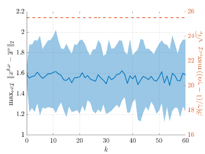
Figure 1: Mean value (solid blue line) and standard deviation (shaded blue area) of the players’ worst-case distance from the continuous equilibrium of the relaxed NEP, computed in those numerical instances for which Algorithm 1 has not converged for MI-NEP ${}^{\text{u}}_{\text{f}}$. The red line denotes, instead, the bound in (14) with $\gamma=1.001$ (note the different values on the left-right ordinates).

While this analysis shows the practical impact of combining Algorithm 1 and 2 with the bound offered in Theorem 3.3, however, we should note that the BR method as described in Algorithm 1 may not necessarily produce a convergent sequence, neither in its Jacobi nor Gauss-Seidel versions (even though the MI-NEP admits at least a MI-NE). In particular, Table 2 shows the percentage of failures declared after $60$ iterations of both versions of Algorithm 1 (actually, $60\cdot N=240$ for the Gauss-Seidel implementation) without computing an MI-NE, established when two consecutive iterations meet the stopping criterion $\|{\bf z}^{k+1}-{\bf z}^{k}\|_{2}\leq 10^{-6}$. In general, we note that the percentage of failures associated to MI-NEP ${}^{\text{t}}_{\text{f}}$ is lower than that of MI-NEP ${}^{\text{u}}_{\text{f}}$. This can be explained as the case with units structurally admits way more combinations of integer feasible points compared to the one with tens, and this behaviour immediately reflects onto the cases considering reduced feasible sets, MI-NEP ${}^{\triangle}_{\text{r}}$, $\triangle\in\{\text{u},\text{t}\}$. In addition, note that the high failure rate shown for MI-NEP ${}^{\text{u}}_{\ast}$, $\ast\in\{\text{f},\text{r}\}$ may be associated with the threshold employed to declare non-convergence, i.e., $60$ iterations. Despite computing a MI-NE via Algorithm 1 with a finer granularity is slightly faster, according to Table 1, it is also more likely to fail. Adopting Algorithm 1 in combination with 2 and the bound in Theorem 3.3 may thus help in reducing the failures potentially occurring when Algorithm 1 is used alone. Considering only those examples for MI-NEP ${}^{\text{u}}_{\text{f}}$ in which convergence has not happened allows us to verify also the bound in Theorem 3.4, as shown in Fig. 1 for $\mathcal{J}^{k}=\mathcal{I}$ – similar results are obtained for the Gauss-Seidel version.

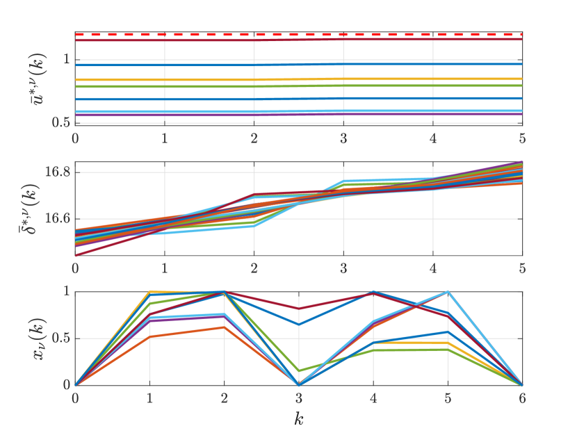
(a)

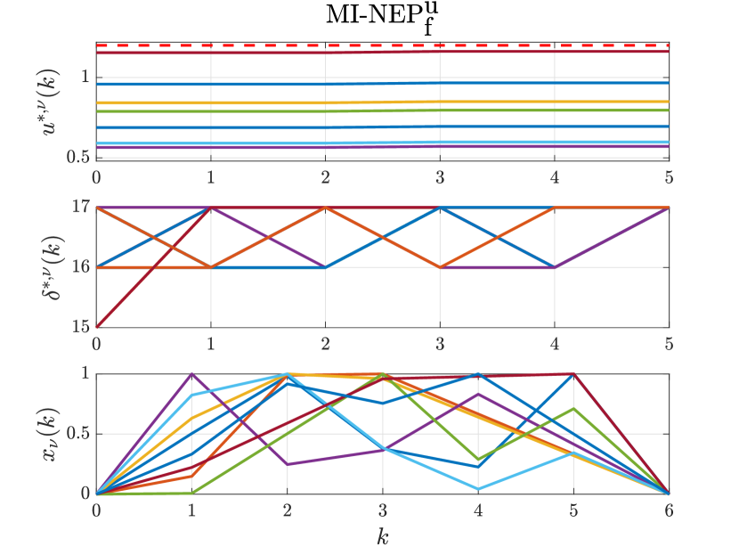
(b)

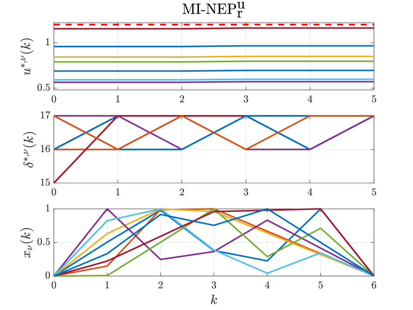
(c)

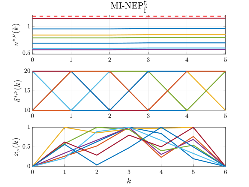
(d)

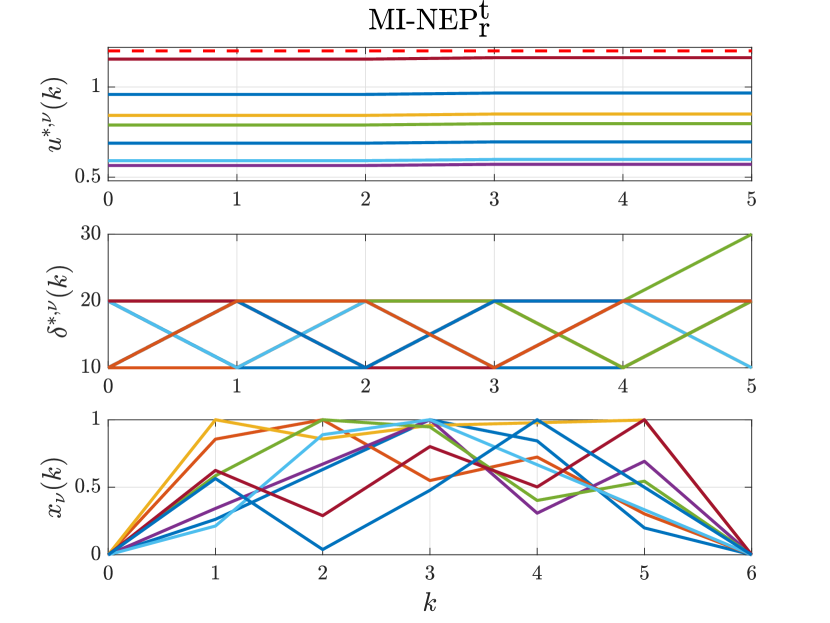
(e)

Figure 2: Example of equilibria computed in all the considered cases. Specifically, (a) Relaxed NEP; MI-NE with granularity up to units over the entire feasible set (b) and over the reduced one (c); MI-NE with granularity up to tens over the entire feasible set (d) and over the reduced one (e).

The plots in Fig. 2, instead, report five equilibria for a numerical instance in which Algorithm 1 with $\mathcal{J}^{k}=\mathcal{I}$, for all $k$, has converged in all the considered cases MI-NEP ${}^{\triangle}_{\ast}$, $\triangle\in\{\text{u},\text{t}\}$, $\ast\in\{\text{f},\text{r}\}$. Relaxing the integer restriction on $\delta^{\nu}(k)$ results in a continuous discharging of the battery, which generates a smoother SOC $x_{\nu}(k)$ in Fig. 2(a) compared to those in Fig. 2(b)–(e). These latter are indeed strictly dependent on the integral restrictions on the scheduling variable $\delta^{\nu}$. In addition, from the evolution of the SOC in Fig. 2(a) we can also appreciate the effect of the daily and night tariffs for energy consumption, which is not so evident with the MI-NE in Fig. 2(b)–(e). While the equilibra computed for the MI-NEP ${}^{\text{u}}_{\ast}$, $\ast\in\{\text{f},\text{r}\}$, in Fig. 2(b)–(c) appear almost coinciding, with a scheduling variable $\delta^{\nu}$ assuming integer values between $15$ and $17$, the equilibria for the cases MI-NEP ${}^{\text{t}}_{\ast}$, $\ast\in\{\text{f},\text{r}\}$, in Fig. 2(d)–(e) instead are substatially different, mostly because $\delta^{\nu}$ varies between $0$ and $40$.

6 Conclusion

Focusing on traditional BR algorithms, we have characterized the convergence properties of the sequence produced in computing solutions to a wide class of MI-NEPs, i.e., problems that turn into monotone NEPs once relaxed the integer restrictions. In particular, we have shown that the resulting sequence always approaches a bounded region containing the entire solution set of the MI-NEP, whose area depends on the problem data. Moreover, we have confirmed that, once a Jacobi/Gauss-Seidel BR method is applied to the relaxed NEP, it converges to the unique solution, and we have also established data-dependent complexity results to characterize its convergence. Nonetheless, we have derived a sufficient condition for the existence of solutions to MI-NEPs, as well as investigated the relation between the contraction property of the continuous NEP and the degree of strong monotonicity possessed by such a relaxed problem. Numerical results on an instance of a smart building control application have illustrated the practical advantages brought by our results.

Future work will be devoted to analyze the numerical benefit entailed by the proposed results when combined with enumerative procedures, as well as to investigate the tight relation between (strong) monotonicity of a MI-NEP and the resulting existence/uniqueness of a solution, thus fully characterizing the connection between Propositions 3 and 1.

Appendix

Proposition 7.

The function $\|\cdot\|^{\cal{B}({\bf w})}$, with ${\bf w}\geq 0$, is a seminorm, namely

1. $\|{\bf z}+{\bf y}\|^{\cal{B}({\bf w})}\leq\|{\bf z}\|^{\cal{B}({\bf w})}+\|{\bf y}\|^{\cal{B}({\bf w})}$ for all ${\bf z},{\bf y}\in{\mathbb{R}}^{n}$,

2. $\|a{\bf z}\|^{\cal{B}({\bf w})}=|a|\|{\bf z}\|^{\cal{B}({\bf w})}$ for all ${\bf z}\in{\mathbb{R}}^{n}$ and $a\in{\mathbb{R}}$.

If ${\bf w}>0$, then $\|\cdot\|^{\cal{B}({\bf w})}$ is a norm, i.e., in addition to (i) and (ii), it satisfies:

1. $\|{\bf z}\|^{\cal{B}({\bf w})}=0$ implies ${\bf z}=0$.

Proof.

(i) Let $\overline{\nu}\in\arg\max_{\nu\in\mathcal{I}}~{}w_{\nu}\|z^{\nu}+y^{\nu}\|$. We have: $\|{\bf z}+{\bf y}\|^{\cal{B}({\bf w})}=w_{\overline{\nu}}\|z^{\overline{\nu}}+y^{\overline{\nu}}\|\leq w_{\overline{\nu}}(\|z^{\overline{\nu}}\|+\|y^{\overline{\nu}}\|)\leq\max_{\nu\in\mathcal{I}}~{}w_{\nu}(\|z^{\nu}\|+\|y^{\nu}\|)=\|{\bf z}\|^{\cal{B}({\bf w})}+\|{\bf y}\|^{\cal{B}({\bf w})}$.

(ii) $\|a{\bf z}\|^{\cal{B}({\bf w})}=\max_{\nu\in\mathcal{I}}~{}w_{\nu}\|az^{\nu}\|=|a|\max_{\nu\in\mathcal{I}}~{}w_{\nu}\|z^{\nu}\|=|a|\|{\bf z}\|^{\cal{B}({\bf w})}.$

(iii) Since ${\bf w}>0$, $\|{\bf z}\|^{\cal{B}({\bf w})}=0\Rightarrow\|z^{\nu}\|=0$, i.e., $z^{\nu}=0$ for all $\nu\in\mathcal{I}$.

References

• (1) Belotti, P., Kirches, C., Leyffer, S., Linderoth, J., Luedtke, J., Mahajan, A.: Mixed-integer nonlinear optimization. Acta Numerica 22, 1–131 (2013)
• (2) Belotti, P., Lee, J., Liberti, L., Margot, F., Wächter, A.: Branching and bounds tightening techniques for non-convex MINLP. Optim. Methods Softw. 24(4-5), 597–634 (2009)
• (3) Bertsekas, D., Tsitziklis, J.: Parallel and Distributed Computation: Numerical Methods. Athena Scientific (1997)
• (4) Bertsekas, D.P.: Nonlinear programming. Journal of the Operational Research Society 48(3), 334–334 (1997)
• (5) Bertsekas, D.P.: Convex optimization algorithms. Athena Scientific Belmont (2015)
• (6) Bigi, G., Lampariello, L., Sagratella, S., Sasso, V.G.: Approximate variational inequalities and equilibria. Computational Management Science 20(1), 43 (2023)
• (7) Cenedese, C., Cucuzzella, M., Scherpen, J., Grammatico, S., Cao, M.: Highway traffic control via smart e-mobility–Part I: Theory. arXiv preprint arXiv:2102.09354 (2021)
• (8) Cenedese, C., Fabiani, F., Cucuzzella, M., Scherpen, J.M., Cao, M., Grammatico, S.: Charging plug-in electric vehicles as a mixed-integer aggregative game. In: 2019 IEEE 58th Conference on Decision and Control (CDC), pp. 4904–4909. IEEE (2019)
• (9) Dreves, A., Facchinei, F., Kanzow, C., Sagratella, S.: On the solution of the KKT conditions of generalized Nash equilibrium problems. SIAM J. Optim. 21(3), 1082–1108 (2011)
• (10) Dreves, A., Sagratella, S.: Nonsingularity and stationarity results for quasi-variational inequalities. Journal of Optimization Theory and Applications 185(3), 711–743 (2020)
• (11) Fabiani, F., Franci, B., Sagratella, S., Schmidt, M., Staudigl, M.: Proximal-like algorithms for equilibrium seeking in mixed-integer Nash equilibrium problems. In: 2022 IEEE 61st Conference on Decision and Control (CDC), pp. 4137–4142. IEEE (2022)
• (12) Fabiani, F., Grammatico, S.: A mixed-logical-dynamical model for automated driving on highways. In: 2018 IEEE Conference on Decision and Control (CDC), pp. 1011–1015. IEEE (2018)
• (13) Fabiani, F., Grammatico, S.: Multi-vehicle automated driving as a generalized mixed-integer potential game. IEEE Transactions on Intelligent Transportation Systems 21(3), 1064–1073 (2019)
• (14) Facchinei, F., Kanzow, C.: Generalized Nash equilibrium problems. Ann. Oper. Res. 175(1), 177–211 (2010)
• (15) Facchinei, F., Pang, J.S.: Finite-Dimensional Variational Inequalities and Complementarity Problems. Springer (2003)
• (16) Grammatico, S.: Dynamic control of agents playing aggregative games with coupling constraints. IEEE Transactions on Automatic Control 62(9), 4537–4548 (2017)
• (17) Gurobi Optimization, LLC: Gurobi Optimizer Reference Manual (2023). URL https://www.gurobi.com
• (18) Löfberg, J.: YALMIP : A toolbox for modeling and optimization in MATLAB. In: In Proceedings of the CACSD Conference. Taipei, Taiwan (2004)
• (19) Nowak, I.: Relaxation and decomposition methods for mixed integer nonlinear programming, vol. 152. Springer Science & Business Media (2006)
• (20) Passacantando, M., Raciti, F.: A finite convergence algorithm for solving linear-quadratic network games with strategic complements and bounded strategies. Optimization Methods and Software pp. 1–24 (2023)
• (21) Sagratella, S.: Computing all solutions of Nash equilibrium problems with discrete strategy sets. SIAM J. Optim. 26(4), 2190–2218 (2016)
• (22) Sagratella, S.: Algorithms for generalized potential games with mixed-integer variables. Computational Optimization and Applications 68(3), 689–717 (2017)
• (23) Sagratella, S.: Computing equilibria of Cournot oligopoly models with mixed-integer quantities. Mathematical Methods of Operations Research 86(3), 549–565 (2017)
• (24) Sagratella, S.: On generalized Nash equilibrium problems with linear coupling constraints and mixed-integer variables. Optimization 68(1), 197–226 (2019)
• (25) Schwarze, S., Stein, O.: A branch-and-prune algorithm for discrete Nash equilibrium problems. Computational Optimization and Applications 86(2), 491–519 (2023)
• (26) Scutari, G., Facchinei, F., Pang, J.S., Palomar, D.P.: Real and complex monotone communication games. IEEE Transactions on Information Theory 60(7), 4197–4231 (2014)
• (27) Scutari, G., Palomar, D.P., Facchinei, F., Pang, J.S.: Monotone games for cognitive radio systems. Distributed decision making and control pp. 83–112 (2012)
• (28) Tawarmalani, M., Sahinidis, N.: Convexification and global optimization in continuous and mixed-integer nonlinear programming: theory, algorithms, software, and applications, vol. 65. Springer Science & Business Media (2002)