From Torch to Projector: Fundamental Tradeoff of Integrated Sensing and Communications

Abstract

snc have been historically developed in parallel. In recent decade, they have been evolving from separation to integration, giving rise to the integrated sensing and communications (ISAC) paradigm, that has been recognized as one of the six key 6G usage scenarios. Despite the plethora of research works dedicated to ISAC signal processing, the fundamental performance limits of sensing and communications (S&C) remain widely unexplored in an ISAC system. In this tutorial paper, we attempt to summarize the recent research findings in characterizing the performance boundary of ISAC systems and the resulting S&C tradeoff from an information-theoretical viewpoint. We begin with a folklore “torch metaphor” that depicts the resource competition mechanism of S&C. Then, we elaborate on the fundamental capacity-distortion (C-D) theory, indicating the incompleteness of this metaphor. Towards that end, we further elaborate on the S&C tradeoff by discussing a special case within the C-D framework, namely the Cramér-Rao bound (CRB)-rate region. In particular, S&C have preference discrepancies over both the subspace occupied by the transmitted signal and the adopted codebook, leading to a “projector metaphor” complementary to the ISAC torch analogy. We also present two practical design examples by leveraging the lessons learned from fundamental theories. Finally, we conclude the paper by identifying a number of open challenges.

I Introduction

ISAC has recently been recognized by the international telecommunication union (ITU) as one of the vertices supporting the 6G hexagon of usage scenarios [1]. By relying on unified hardware platforms and radio waveforms, such integration enables resource-efficient cooperation between S&C subsystems, supporting various emerging applications including vehicular-to-everything (V2X) networking, extended reality (XR), and digital twins.

Early endeavours on ISAC system design aim to extend the capability of existing infrastructures, hence developed into sensing-centric and communication-centric paradigms. Representative sensing-centric schemes include communicating using radar sidelobes and the permutation degree of freedom (DoF) in the waveform-antenna mapping of multiple-input multiple-output (MIMO) radars [2]. Communication-centric schemes are exemplified by sensing relying on orthogonal frequency-division multiplexing (OFDM) waveforms [3]. These schemes do not target the optimal S&C performance. To push the benefit of ISAC (termed as the “integration gain” [4]) to its limit, joint design schemes emerged more recently [5], which aim at conceiving novel joint signaling strategies from the ground-up, capable of accomplishing both tasks simultaneously. A natural, but easily overlooked question that arises is: What is the fundamental limit of the integration gain?

If we focus back on conventional individual S&C systems, we see that their fundamental performance limits originate from the resource budget. For example, the celebrated Shannon capacity formula for the scalar Gaussian channel exactly expresses the dependency of the communication performance on the available power and bandwidth. However, the performance limit of ISAC systems is vastly different. In its essence, the problem of ISAC system design is a multi-objective optimization problem. To elaborate, separated S&C design can be viewed as a special case of ISAC design, namely employing a time-sharing strategy. By utilizing the synergies between S&C, more favorable performance can be achieved. However, besides some rare occasions, it is highly unlikely that S&C would achieve their optimal performance at the same time, suggesting the existence of a fundamental S&C tradeoff in an ISAC system. Such a tradeoff may be framed by the Pareto boundary of the multi-objective ISAC system design problem.

For decades, S&C have been regarded as an information-theoretical “odd couple” that are mutually intertwined in profound ways [6]. At large, the S&C tradeoff may be understood from the perspective of a signal-and-system duality. For instance, let us consider a simple linear Gaussian model given by

$$\bm{\mathsfbr{Y}}=\bm{\mathsfbr{H}}\bm{\mathsfbr{X}}+\bm{\mathsfbr{Z}}$$ (1)

with $\bm{\mathsfbr{X}}$, $\bm{\mathsfbr{Y}}$, $\bm{\mathsfbr{H}}$ and $\bm{\mathsfbr{Z}}$ being the transmitted ISAC signal, the received signal, the channel, and the noise, respectively. For communication, the task is to decode the message encoded in $\bm{\mathsfbr{X}}$, whereas for sensing, the task is to extract information from the channel $\bm{\mathsfbr{H}}$. In light of this, one may view $\bm{\mathsfbr{H}}$ as the “transmitted signal” from the environment to be sensed, while viewing $\bm{\mathsfbr{X}}$ as the “channel’ that this “signal” would pass through.

While the connection between estimation and information theories has been well-studied in the context of, e.g., I-MMSE equation [7], the fundamental tradeoff still remains widely open in general. To this end, this article will summarize current understandings of different components in the S&C tradeoff in a coherent manner, through the prism of information theory [8, 9, 10, 11, 12]. We shall commence with a folklore “torch metaphor” depicting the resource competition between S&C subsystems, followed by the general capacity-distortion theory suggesting the incompleteness of this metaphor. We then introduce the CRB-rate region which clearly indicates that the S&C tradeoff is two-fold: Apart from resources, S&C subsystems would also have different preferences on the input distribution. For each component in this tradeoff, we provide design examples illustrating its practical implications. Finally, we conclude this paper with some open challenges.

II The Torch Metaphor

The fundamental S&C tradeoff in ISAC has been exemplified (implicitly or explicitly) by the “torch metaphor” in some works [13, 5], as illustrated in Fig. 1. In this picture, the role played by the ISAC base station (BS) resembles a child holding a torch: If she points the torch towards the communication user, the user would receive the message, while the sensing target is left in the dark and hence can hardly be seen. On the other hand, if the target is maximally illuminated, the user would receive very weak signals, resulting in highly noise-corrupted messages. This metaphor is intuitive, and it provides us with the following basic understandings of the S&C tradeoff:

• Power allocation across orthogonal or quasi-orthogonal dimensions (in the case of Fig. 1 it is space, or angle, but it could be time, or frequency) offers an immediate way to tradeoff communication and sensing performance;

• Since we are using a unified signal, when the communication user and the sensing target are “close to each other”, the S&C tradeoff becomes less prominent.

Inspired by these intuitions, most existing research contributions on ISAC system design focus on power allocation in a generalized sense, including beamforming in MIMO systems [5] and subcarrier power allocation in OFDM systems [14]. Despite the effectiveness of these techniques, we would still wonder, whether the torch metaphor depicts the full picture of the S&C tradeoff.

Recently, it has been found that the torch metaphor does cover the full picture, when the sensing task is to detect the presence of a potential target, under some specific choice of sensing performance metrics [12]. Specifically, in this scenario, during the $n$-th channel use, the ISAC BS would determine the absence/presence of the target (represented by a state $\seta\in\{0,1\}$) based on an echo $\bm{\mathsfbr{Y}}_{{\rm s},n}$, while the user aims for decoding the information conveyed in the transmitted ISAC signal $\bm{\mathsfbr{X}}_{n}$, based on its received signal $\bm{\mathsfbr{Y}}_{{\rm c},n}$. Both the echo and the user-received signal are contaminated by circularly symmetric Gaussian noises, denoted by $\bm{\mathsfbr{Z}}_{{\rm s},n}$ and $\bm{\mathsfbr{Z}}_{{\rm c},n}$, respectively. Such a scenario may be characterized as

$$\bm{\mathsfbr{Y}}_{{\rm c},n} =\bm{H}_{\rm c}\bm{\mathsfbr{X}}_{n}+\bm{\mathsfbr{Z}}_{{\rm c},n},$$ (2a)

$$\bm{\mathsfbr{Y}}_{{\rm s},n} =\seta\bm{H}_{\rm s}\bm{\mathsfbr{X}}_{n}+\bm{\mathsfbr{Z}}_{{\rm s},n},$$ (2b)

where $n=1,2,\dotsc,N$, $N$ is the coding block length, $\bm{H}_{\rm c}$ denotes the communication channel, while $\bm{H}_{\rm s}$ represents the target response matrix (also referred to as the sensing channel [10, 11, 12]). For communication, a natural performance metric is the communication rate given by

$$R=\lim_{N\rightarrow\infty}\frac{1}{N}\log M_{N},$$

under the assumption that the decoding error probability vanishes as $N$ tends to infinity, and $M_{N}$ denotes the size of the communication codebook. For sensing, the performance metric chosen in [12, 15] is the error exponent defined as

$$E=\lim_{N\rightarrow\infty}\frac{1}{N}\log\frac{1}{\delta_{N}},$$ (3)

where $\delta_{N}$ denotes the maximum detection error probability over all codewords and target states, namely

$$\delta_{N}=\max_{w\in[M_{N}]}\max_{s\in\{0,1\}}\mathbb{P}\left\{\hat{S}\left(\bm{\mathsfbr{Y}}_{\rm s}^{N},\bm{\mathsfbr{X}}^{N}(\mathsfbr{W})\right)\neq\seta|\seta=s,\mathsfbr{W}=w\right\},$$

with $\mathsfbr{W}\in[M_{N}]$ being the encoded message, $\bm{\mathsfbr{Y}}_{\rm s}^{N}\!=\!\{\bm{\mathsfbr{Y}}_{{\rm s},1},\bm{\mathsfbr{Y}}_{{\rm s},2},\dotsc,\bm{\mathsfbr{Y}}_{{\rm s},N}\}$, and $\bm{\mathsfbr{X}}^{N}(W)\!=\!\{\bm{\mathsfbr{X}}_{1},\bm{\mathsfbr{X}}_{2},\dotsc,\bm{\mathsfbr{X}}_{N}\}$. Under the aforementioned setting, the set constituted by all achievable $(R,E)$ pairs (termed as the rate-exponent region) is shown to be characterized by [12]

$$R \leqslant\log\left|\bm{I}+\sigma_{\rm c}^{-2}\bm{H}_{\rm c}\widetilde{\bm{R}}_{\bm{\mathsfbr{X}}}\bm{H}_{\rm c}^{\rm H}\right|,$$ (4a)

$$E \leqslant\frac{1}{4}{\rm Tr}\left\{\sigma_{\rm s}^{-2}\bm{H}_{\rm s}\widetilde{\bm{R}}_{\bm{\mathsfbr{X}}}\bm{H}_{\rm s}^{\rm H}\right\},$$ (4b)

where $\widetilde{\bm{R}}_{\bm{\mathsfbr{X}}}=\mathbb{E}\left\{\frac{1}{N}\sum_{n=1}^{N}\bm{\mathsfbr{X}}_{n}\bm{\mathsfbr{X}}_{n}^{\rm H}\right\}$ is the statistical covariance matrix of the transmitted ISAC signal, satisfying a power budget constraint ${\rm Tr}\{\widetilde{\bm{R}}_{\bm{\mathsfbr{X}}}\}\leqslant P$.

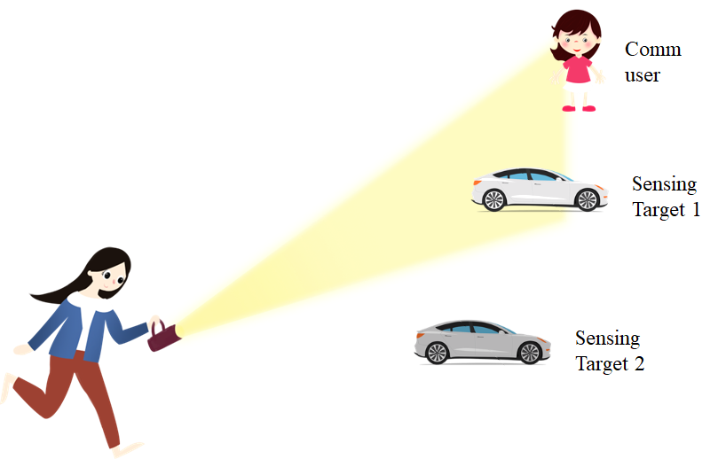
Figure 1: Graphical illustration of the torch metaphor.

From (4) we observe a concrete version of the torch metaphor. Apparently, the communication-optimal $\widetilde{\bm{R}}_{\bm{\mathsfbr{X}}}$ would have its eigenvectors matching those of $\bm{H}_{\rm c}$, while the eigenvalues determined by the water-filling power allocation [16]. By contrast, the sensing-optimal $\widetilde{\bm{R}}_{\bm{\mathsfbr{X}}}$ would be aligned with the dominant eigenvector (possibly having multiplicity larger than $1$) of $\bm{H}_{\rm s}$ [12]. Therefore, as long as the eigenspaces of $\bm{H}_{\rm s}$ and $\bm{H}_{\rm c}$ do not match, or the water-filling strategy does not concentrate the power on the dominant eigenvector, there would be a S&C tradeoff. Furthermore, (4) also gives us an explicit sense in which the communication user and the sensing target are “close to each other”: their distance may be characterized by a measure of discrepancy between the “communication subspace” ${\rm span}(\bm{H}_{\rm c})$ and the “sensing subspace” – the dominant eigenvector of $\bm{H}_{\rm s}$. In light of this, such a tradeoff is termed as the subspace tradeoff (ST) in [10], and thus the torch metaphor may be represented concisely as the statement of

$$\mathrm{S\&C}\leavevmode\nobreak\ {\rm tradeoff}=\mathrm{ST}.$$ (5)

To further reveal the nature of the ST, let us consider a tangible example, in which the BS is equipped with collocated transmit and receive uniform linear antenna arrays (half-wavelength spacing) of the size $N_{\rm s}=M=10$, the user has a single antenna (i.e. $N_{\rm c}=1$), while the sensing target is point-like. In this scenario, the communication and sensing channels are given by

$$\bm{H}_{\rm c}=\alpha_{\rm c}\bm{a}^{\rm H}(\theta_{\rm c}),\leavevmode\nobreak\ \leavevmode\nobreak\ \bm{H}_{\rm s}=\alpha_{\rm s}\bm{a}(\theta_{\rm s})\bm{a}^{\rm H}(\theta_{\rm s}),$$

where $\alpha_{\rm c}$ and $\alpha_{\rm s}$ denote the scalar channel coefficients, $\theta_{\rm c}$ and $\theta_{\rm s}$ denote the bearing angle of the user and the target relative to the BS, respectively, while $\bm{a}(\theta)$ is the array steering vector given by

$$\bm{a}(\theta)=[1,\leavevmode\nobreak\ e^{j\pi\sin(\theta)},\leavevmode\nobreak\ e^{j2\pi\sin(\theta)},\dotsc,e^{j\pi(N_{\rm s}-1)\sin(\theta)}]^{\rm T}.$$

Correspondingly, the characterization of the rate-exponent region (4) can then be simplified as

$$\bm{r}(\lambda) \!=\!\mathop{\rm argmax}_{\bm{v}:\|\bm{v}\|=1}\leavevmode\nobreak\ (1\!-\!\lambda)|\bm{v}^{\rm H}\bm{a}(\theta_{\rm c})|^{2}\!+\!\lambda|\bm{v}^{\rm H}\bm{a}(\theta_{\rm s})|^{2},\leavevmode\nobreak\ \lambda\!\in\![0,1]$$ (6a)

$$R(\lambda) \!\leqslant\!\log(1+P\sigma_{\rm c}^{-2}|\alpha_{\rm c}|^{2}|\bm{r}^{\rm H}(\lambda)\bm{a}(\theta_{\rm c})|^{2}),$$ (6b)

$$E(\lambda) \!\leqslant\!\frac{1}{4}{\rm Tr}\left\{P\sigma_{\rm s}^{-2}|\alpha_{\rm s}|^{2}|\bm{r}^{\rm H}(\lambda)\bm{a}(\theta_{\rm s})|^{2}\right\},$$ (6c)

where $\lambda$ is a parameter controlling the S&C tradeoff. The communication and sensing signal-to-noise ratios may be expressed as

$${\rm SNR}_{\rm c}=P\|\bm{H}_{\rm c}\|_{\rm F}^{2}\sigma_{\rm c}^{-2},\leavevmode\nobreak\ \leavevmode\nobreak\ {\rm SNR}_{\rm s}=P\|\bm{H}_{\rm s}\|_{\rm F}^{2}\sigma_{\rm s}^{-2}.$$

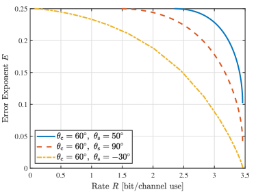
Figure 2: The rate-exponent region of the single-antenna user, point-like target scenario, with communication and sensing SNRs equal to $10$dB and $0$dB, respectively.

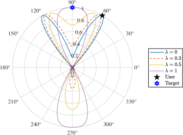
(a) $\theta_{\rm c}=60^{\circ},\leavevmode\nobreak\ \theta_{\rm s}=90^{\circ}$

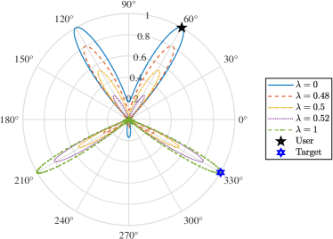
(b) $\theta_{\rm c}=60^{\circ},\leavevmode\nobreak\ \theta_{\rm s}=-30^{\circ}$

Figure 3: Beamspace illustration of the subspace tradeoff (corresponding to the rate-exponent regions in Fig. 2). The “ISAC torch” can simultaneously illuminate both the user and the target in case (a), while it has to apply a power-splitting strategy in case (b).

Using (6), we may readily obtain the rate-exponent regions for given configurations of $(\theta_{\rm c},\theta_{\rm s})$, as portrayed in Fig. 2. Note that the closeness between the S&C subspaces in this scenario is characterized by the intersection angle between $\bm{a}(\theta_{\rm c})$ and $\bm{a}(\theta_{\rm s})$. We may observe from Fig. 2 that the S&C tradeoff becomes more prominent as the angular separation between the target and the user increases. More intuitively, as can be seen from Fig. 2, in the $\theta_{\rm c}=60^{\circ}$, $\theta_{\rm s}=90^{\circ}$ scenario, the sensing-optimal and communication-optimal beam patterns (corresponding to $\lambda=0$ and $\lambda=1$, respectively) have a large overlap. By contrast, in the $\theta_{\rm c}=60^{\circ}$, $\theta_{\rm s}=-30^{\circ}$ scenario, the sensing- and communication-optimal beam patterns are almost orthogonal to each other. This corroborates our intuition about the ST, that more synergies between S&C tasks would be witnessed as the corresponding subspaces become closer to each other. In the language of the torch metaphor, we may say that the “ISAC torch” in the case of Fig. 3a can simultaneously illuminate both the user and the target, while it has to apply a power-splitting strategy in the case of Fig. 3b.

Now that we see (5) holds true for the target presence detection problem under the sensing metric of error exponent, we would naturally ask in the sequel that:

• Does (5) hold in general?

• If not, what is the key condition for (5) to hold? Is it the metric chosen (error exponent), the specific type of the sensing task (target detection), or both?

III Capacity-Distortion Theory

To answer these questions, one has to rely on a more general analytical framework, that applies to both estimation and detection tasks and can handle favorably all reasonable sensing performance metrics. The capacity-distortion theory [8, 9, 10] is conceived in the hope of building such a universal framework.

III-A Rate-Distortion Region

As the name suggests, the capacity-distortion theory investigates the tradeoff between communication capacity and sensing distortion. Originally proposed by Shannon in the context of rate-distortion theory for lossy data compression [17], distortion refers to a wide range of functions taking the form of $d(\bm{\seta},\hat{\bm{\seta}})$, whose inputs are the true value of some quantity (in sensing problems, the sensing parameter) $\bm{\seta}$ and its estimate $\hat{\bm{\seta}}$. Due to the randomness of the communication message, the ISAC waveform (codeword) $\bm{\mathsfbr{X}}^{N}$ is also random. To reflect the sensing performance over a relatively long period of time, a common practice is to use the expectation of the distortion, instead of its instantaneous values, as the performance metric. For example, in estimation tasks, the squared Euclidean distance $d(\bm{\seta},\hat{\bm{\seta}})=\|\bm{\seta}-\hat{\bm{\seta}}\|^{2}$ is a widely applied distortion function, whose expectation is the mean-squared error (MSE). In binary (e.g. target presence) detection problems in which the task is to determine the value of a binary variable $\seta\in\{0,1\}$, a valid distortion function is the Hamming distance given by $d(\seta,\hat{\seta})=\seta\oplus\hat{\seta}$, whose expectation is related to commonly used detection metrics, including the detection probability $P_{\rm D}$ and the false alarm rate $P_{\rm FA}$, as follows:

$$\mathbb{E}\{\seta\oplus\hat{\seta}\}$$

$$\hskip 8.53581pt=(1\oplus 1)\mathbb{P}\{\hat{\seta}=1|\seta=1\}+(0\oplus 0)\mathbb{P}\{\hat{\seta}=0|\seta=0\}$$

$$\hskip 19.91692pt+(1\oplus 0)\mathbb{P}\{\hat{\seta}=1|\seta=0\}+(0\oplus 1)\mathbb{P}\{\hat{\seta}=0|\seta=1\}$$

$$\hskip 8.53581pt=1-P_{\rm D}+P_{\rm FA}.$$ (7)

Note that for constant false-alarm rate (CFAR) detectors based on the Neyman-Pearson criterion with fixed $P_{\rm FA}$ [18], minimizing the Hamming distance is equivalent to maximizing the detection probability $P_{\rm D}$.

Besides capacity and distortion, there is yet another important ingredient in the capacity-distortion theory, namely the transmission cost. To elaborate, not all ISAC waveforms (or codewords) cost equally in terms of wireless resources. For example, the points in quadrature amplitude modulation (QAM) constellations having different amplitudes would yield different power consumptions. Apparently, as the overall resource budget increases, S&C performances can be simultaneously enhanced. Therefore, one has to discuss the capacity-distortion tradeoff under a specific resource budget. Similar to the sensing distortion, in order to take into account the randomness of the codewords, we typically use the expectation of the resource cost over all possible codewords as the measure of transmission cost.

Once the resource budget is given and the sensing distortion metric is chosen, the S&C tradeoff is expressed in terms of the largest achievable rate-distortion region. Formally speaking, given an expected resource budget $B$, the rate-distortion-cost triple $(R,D,B)$ is said to be achievable (in the infinite block length regime), if there exists a sequence of $(2^{NR},R)$ codes $\{\bm{\mathsfbr{X}}^{N}|N\in\mathbb{N}\}$ encoding the message $\mathsfbr{W}\in\{1,\dotsc,2^{NR}\}$, and a state estimator function $\hat{\bm{\seta}}:(\bm{\mathsfbr{Y}}_{\rm s},\bm{\mathsfbr{X}}^{N})\mapsto\hat{\bm{\seta}}$, such that the following holds [10]

$$\mathbb{E}\big{\{}d\big{(}\bm{\seta}^{N},\hat{\bm{\seta}}^{N}\big{)}\big{\}}\leqslant D,$$ (8a)

$$\mathbb{E}\{b(\bm{\mathsfbr{X}}^{N})\}\leqslant B,$$ (8b)

$$P_{\rm e}^{(N)}:=\frac{1}{2^{NR}}\sum_{i=1}^{2^{NR}}\mathbb{P}\{\hat{\mathsfbr{W}}\neq i|\mathsfbr{W}=i\}\rightarrow 0,$$ (8c)

as $N\rightarrow\infty$, where $b(\cdot)$ denotes the instantaneous cost of single codeword. In addition, for generality, the values of the sensing parameters are allowed to vary across time, denoted by $\bm{\seta}_{i}$ at the $i$-th channel use, constituting a parameter sequence $\bm{\seta}^{N}$. The capacity-distortion function given a specific resource budget $B$ is then defined as

$$C_{B}(D)=\sup\{R|(R,D,B)\leavevmode\nobreak\ \textrm{is\leavevmode\nobreak\ achievable}\}.$$ (9)

\begin{overpic}[width=199.4681pt]{figures/general_CD_model2.eps} \put(42.2,16.0){\footnotesize$P_{\bm{\mathsfbr{Y}}_{\rm s},\bm{\mathsfbr{Y}}_{\rm c}|\bm{\mathsfbr{X}},\bm{\seta}}$} \put(3.0,18.0){\footnotesize$\mathsfbr{W}$} \put(29.5,17.5){\footnotesize$\bm{\mathsfbr{X}}_{i}$} \put(61.0,25.0){\footnotesize$\bm{\mathsfbr{Y}}_{{\rm s},i}$} \put(61.0,14.0){\footnotesize$\bm{\mathsfbr{Y}}_{{\rm c},i}$} \put(93.0,7.5){\footnotesize$\hat{\mathsfbr{W}}$} \put(93.5,28.0){\footnotesize$\hat{\bm{\seta}}_{i}$} \put(48.0,2.0){\footnotesize$P_{\bm{\seta}}$} \put(62.0,4.5){\footnotesize$\bm{\seta}_{i}$} \end{overpic}

Figure 4: The structure of a generic ISAC system with memoryless channels, often considered in the capacity-distortion theory.

For the simplicity of discussion, let us consider memoryless channels, exemplified by (2), and illustrated in Fig. 4. The effect of such channels can be expressed as

$$p_{\mathsfbr{W},\bm{\mathsfbr{Y}}_{\rm c}^{N},\bm{\mathsfbr{Y}}_{\rm s}^{N},\bm{\mathsfbr{X}}^{N},\bm{\seta}^{N}}(W,\bm{Y}_{\rm s},\bm{Y}_{\rm c},\bm{X},\bm{\eta})=p_{\mathsfbr{W}}(W)$$

$$\hskip 8.53581pt\times\prod_{i=1}^{N}p_{\bm{\seta}}(\bm{\eta}_{i})p_{\bm{\mathsfbr{X}}|\mathsfbr{W}}(\bm{X}_{i}|\mathsfbr{W})p_{\bm{\mathsfbr{Y}}_{\rm s},\bm{\mathsfbr{Y}}_{\rm c}|\bm{\mathsfbr{X}},\bm{\seta}}(\bm{Y}_{{\rm s},i},\bm{Y}_{{\rm c},i}|\bm{X}_{i},\bm{\eta}_{i}).$$ (10)

In particular, the channel $p_{\mathsfbr{W},\bm{\mathsfbr{Y}}_{\rm c}^{N},\bm{\mathsfbr{Y}}_{\rm s}^{N},\bm{\mathsfbr{X}}^{N},\bm{\seta}^{N}}(W,\bm{Y}_{\rm s},\bm{Y}_{\rm c},\bm{X},\bm{\eta})$ produces a communication output $\bm{\mathsfbr{Y}}_{\rm c}$ and a sensing output $\bm{\mathsfbr{Y}}_{\rm s}$, whereas their relationship with the channel input $\bm{\mathsfbr{X}}$ can be different from the linear model (2). Moreover, the way that the sensing parameter $\bm{\seta}$ couples with the channel can also be different. For such channels, it is natural to consider per-block resource budgets and distortion metrics, given by

$$\mathbb{E}\big{\{}b\big{(}\bm{\mathsfbr{X}}^{N}\big{)}\big{\}} =\frac{1}{N}\sum_{n=1}^{N}\mathbb{E}\{b(\bm{\mathsfbr{X}}_{i})\},$$

$$\mathbb{E}\big{\{}d\big{(}\bm{\seta}^{N},\hat{\bm{\seta}}^{N}\big{)}\big{\}} =\frac{1}{N}\sum_{n=1}^{N}\mathbb{E}\{d(\bm{\seta}_{i},\hat{\bm{\seta}}_{i})\}.$$

The conditions (8) can then be concretized as

$$\limsup_{N\rightarrow\infty}\leavevmode\nobreak\ \frac{1}{N}\sum_{n=1}^{N}\mathbb{E}\{d(\bm{\seta}_{i},\hat{\bm{\seta}}_{i})\} \leqslant D,$$ (11a)

$$\limsup_{N\rightarrow\infty}\leavevmode\nobreak\ \frac{1}{N}\sum_{n=1}^{N}\mathbb{E}\{b(\bm{\mathsfbr{X}}_{i})\} \leqslant B,$$ (11b)

$$\limsup_{N\rightarrow\infty}\leavevmode\nobreak\ P_{\rm e}^{(N)} =0.$$ (11c)

In order to gain insights from (11), observe that when the sensing distortion constraint (11a) is absent, the capacity is given by the classical result of “capacity-with-cost” [20]

$$C_{B}=\max_{p_{\bm{\mathsfbr{X}}}(\bm{X})\in{\cal{P}}_{B}}\leavevmode\nobreak\ \leavevmode\nobreak\ I(\bm{\mathsfbr{X}};\bm{\mathsfbr{Y}}_{\rm c}),$$ (12)

where

$${\cal{P}}_{B}=\{p_{\bm{\mathsfbr{X}}}(\bm{X})|\mathbb{E}\{b(\bm{\mathsfbr{X}})\}\leqslant B\}.$$

The result (12) implies that the capacity in the presence of cost budget has a single-letter representation, which would extremely simplify further analysis. Furthermore, since the sensing channel is memoryless, the optimal estimator does not rely on historical observations, and hence the expected distortion can be written as a function of the channel input, i.e. $\mathbb{E}\{d(\bm{\seta}_{i},\hat{\bm{\seta}}_{i})|\bm{\mathsfbr{X}}=\bm{X}\}=c(\bm{X})$. In light of this, the capacity-distortion function can now be viewed as a capacity with two costs, namely [10]

$$C_{B}(D) =\sup_{p_{\bm{\mathsfbr{X}}}(\bm{X})\in{\cal{P}}_{B}\cap{\cal{P}}_{D}}\leavevmode\nobreak\ I(\bm{\mathsfbr{X}};\bm{\mathsfbr{Y}}_{\rm c}|\bm{\seta}),$$ (13a)

$${\cal{P}}_{B} =\{p_{\bm{\mathsfbr{X}}}(\bm{X})|\mathbb{E}\{b(\bm{\mathsfbr{X}})\}\leqslant B\},$$ (13b)

$${\cal{P}}_{D} =\{p_{\bm{\mathsfbr{X}}}(\bm{X})|\mathbb{E}\{c(\bm{\mathsfbr{X}})\}\leqslant D\}.$$ (13c)

Remarkably, the result (13) suggests that the expected sensing distortion may be alternatively viewed as a kind of “sensing-induced communication cost”. This understanding enables us to extend even further the range that the capacity-distortion theory is applicable, to scenarios in which the sensing performance cannot be described by a proper distortion function. For example, the Cramér-Rao bound (CRB) widely used as the performance metric of estimation problems is not dependent on any specific estimator $\hat{\bm{\seta}}$. Sometimes it does not even depend on the true value of the parameter $\bm{\seta}$. Therefore, CRB is not a distortion function, but it is related to the transmitted codeword $\bm{\mathsfbr{X}}$ (as will be discussed later), and hence the capacity-distortion theory can still be applied in the generalized sense.

In this aforementioned scenario, we did not consider feedback. One may wonder whether designing the ISAC codebook by relying on feedback can further enhance the S&C performance. To this end, the state-dependent memoryless channel with delayed feedback (SDMC-DF) model has been investigated [10]. The effect of an SDMC-DF can be expressed as [8]

$$p_{\mathsfbr{W},\bm{\mathsfbr{Y}}^{N},\bm{\mathsfbr{Z}}^{N},\bm{\mathsfbr{X}}^{N},\bm{\seta}^{N}}(W,\bm{Y},\bm{Z},\bm{X},\bm{\eta})=p_{\mathsfbr{W}}(W)$$

$$\hskip 2.84526pt\times\!\prod_{i=1}^{N}p_{\bm{\seta}}(\bm{\eta}_{i})p_{\bm{\mathsfbr{X}}|\mathsfbr{W},\bm{\mathsfbr{Z}}}(\bm{X}_{i}|\mathsfbr{W},\!\bm{Z}_{i-1})p_{\bm{\mathsfbr{Y}},\bm{\mathsfbr{Z}}|\bm{\mathsfbr{X}},\bm{\seta}}(\bm{Y}_{i},\!\bm{Z}_{i}|\bm{X}_{i},\!\bm{\eta}_{i})$$ (14)

where both sensing and communication rely on the same channel, which produces the output $\bm{\mathsfbr{Y}}^{N}$. For sensing tasks, the channel input $\bm{\mathsfbr{X}}_{i}$ at the $i$-th channel use cannot be designed based on the real-time channel output $\bm{\mathsfbr{Y}}_{i}$ or the parameter value $\bm{\seta}_{i}$, since the design process has to be causal. Rather, one can only rely on a delayed feedback $\bm{\mathsfbr{Z}}_{i-1}$, which may be a function of the channel output $\bm{\mathsfbr{Y}}_{i}$.

It turns out that, for SDMC-DF models, (13) also applies, with the slight modification that $\bm{\mathsfbr{Y}}_{\rm c}$ is replaced with $\bm{\mathsfbr{Y}}$. To see this, first note that feedback does not improve the capacity of memoryless channels. For the sensing performance, it has been shown that the optimal sensing distortion is achievable by the simple letter-wise minimum expected posterior distortion estimator [10] taking the form of

$$\gamma(\bm{\mathsfbr{X}},\bm{\mathsfbr{Z}})=\left(\hat{\bm{\seta}}^{\ast}(\bm{\mathsfbr{X}}_{1},\bm{\mathsfbr{Z}}_{1}),\dotsc,\hat{\bm{\seta}}^{\ast}(\bm{\mathsfbr{X}}_{N},\bm{\mathsfbr{Z}}_{N})\right),$$

where

$$\hat{\bm{\seta}}^{\ast}(\bm{X},\bm{Z})=\mathop{\arg\min}_{\bm{\seta}^{\prime}}\leavevmode\nobreak\ \int d(\bm{\seta},\bm{\seta}^{\prime})p_{\bm{\seta}|\bm{\mathsfbr{X}},\bm{\mathsfbr{Z}}}(\bm{\eta}|\bm{X},\bm{Z}){\rm d}\bm{\eta}.$$

We may now see that the expected distortion also admits a single-letter representation

$$c(\bm{X})=\mathbb{E}\big{\{}d\big{(}\bm{\seta},\hat{\bm{\seta}}^{\ast}(\bm{\mathsfbr{X}},\bm{\mathsfbr{Z}})\big{)}|\bm{\mathsfbr{X}}=\bm{X}\big{\}},$$ (15)

and thus (13) still applies.

From the aforementioned discussion, we may conclude that a key condition for (13) to hold is the memorylessness of channels. Indeed, for channels with memory, even the capacity itself remains open. Furthermore, for such channels, online and offline estimators may have very different performances. These problems deserve further investigation.

III-B Computing the Capacity-Distortion Boundary

From a pure theorist’s perspective, the result (13) is a complete information characterization (as opposed to the operational definition (11)) of the capacity-distortion region. But wait! Remember that our expectation on the capacity-distortion theory in the first place was to help understand the nature of the S&C tradeoff, hopefully beyond the ST. However, we cannot even dig ST itself out of (13), not to mention any further insight.

To serve our purpose, a possible approach is to compute explicitly the capacity-distortion functions for some representative scenarios, in the hope of obtaining useful intuitions. It turns out that the renowned Blahut-Arimoto (B-A) algorithm [21] originally proposed for computing the unconstrained capacity can be applied to compute capacity-distortion functions with some modifications. To elaborate, given an initialization of the trail distribution $r(\bm{X})$ for $p_{\bm{\mathsfbr{X}}}(\bm{X})$, the original B-A algorithm solving $C=\max_{p_{\bm{\mathsfbr{X}}}(\bm{X})}\leavevmode\nobreak\ I(\bm{\mathsfbr{X}};\bm{\mathsfbr{Y}})$ is a fixed-point iteration repeating the following two steps in each round:

1. Update the trail distribution $q(\bm{X}|\bm{Y})$ for the a posteriori distribution $p_{\bm{\mathsfbr{X}}|\bm{\mathsfbr{Y}}}(\bm{X}|\bm{Y})$ according to

   $$q(\bm{X}|\bm{Y})\leftarrow\frac{p_{\bm{\mathsfbr{X}}}(\bm{X})p_{\bm{\mathsfbr{Y}}|\bm{\mathsfbr{X}}}(\bm{Y}|\bm{X})}{\int r(\bm{X})p_{\bm{\mathsfbr{Y}}|\bm{\mathsfbr{X}}}(\bm{Y}|\bm{X}){\rm d}\bm{X}};$$ (16)

2. Update $r(\bm{X})$ by

   $$r(\bm{X})\leftarrow\frac{e^{\int p_{\bm{\mathsfbr{Y}}|\bm{\mathsfbr{X}}}(\bm{Y}|\bm{X})\log q(\bm{X}|\bm{Y}){\rm d}\bm{Y}}}{\int e^{\int p_{\bm{\mathsfbr{Y}}|\bm{\mathsfbr{X}}}(\bm{Y}|\bm{X})\log q(\bm{X}|\bm{Y}){\rm d}\bm{Y}}{\rm d}\bm{X}},$$ (17)

   which is equivalent to solving the following constrained entropy maximization problem:

   $$r(\bm{X})\leftarrow \mathop{\arg\max}_{p(\bm{X})}-\int p(\bm{X})\log p(\bm{X}){\rm d}\bm{X},$$

   $${\rm s.t.}\leavevmode\nobreak\ p(\bm{X})\geqslant 0\leavevmode\nobreak\ \forall\bm{X},\leavevmode\nobreak\ \int p(\bm{X}){\rm d}\bm{X}=1,$$

   $$\mathbb{E}_{p(\bm{X})}\Big{\{}\int p_{\bm{\mathsfbr{Y}}|\bm{\mathsfbr{X}}}(\bm{Y}|\bm{X})\log q(\bm{X}|\bm{Y}){\rm d}\bm{Y}\Big{\}}\geqslant t$$

   for some constant $t$.

Now that our objective function is the conditional mutual information $I(\bm{\mathsfbr{X}};\bm{\mathsfbr{Y}}|\bm{\seta})$, we shall replace (16) with

$$q(\bm{X}|\bm{Y},\bm{\eta})\leftarrow\frac{p_{\bm{\mathsfbr{X}}}(\bm{X})p_{\bm{\mathsfbr{Y}}|\bm{\mathsfbr{X}},\bm{\seta}}(\bm{Y}|\bm{X},\bm{\eta})}{\int p_{\bm{\mathsfbr{X}}}(\bm{X})p_{\bm{\mathsfbr{Y}}|\bm{\mathsfbr{X}},\bm{\seta}}(\bm{Y}|\bm{X},\bm{\eta}){\rm d}\bm{X}}.$$

In addition, since two extra constraints (13b) and (13c) are now enforced, we should replace (17) with

$$r(\bm{X})\leftarrow$$

$$\hskip 8.53581pt\frac{e^{\int[p_{\bm{\seta}}(\bm{\eta})p_{\bm{\mathsfbr{Y}}|\bm{\mathsfbr{X}},\bm{\seta}}(\bm{Y}|\bm{X},\bm{\eta})\log q(\bm{X}|\bm{Y},\bm{\eta})-\lambda b(\bm{X})-\mu c(\bm{X})]{\rm d}\bm{\eta}{\rm d}\bm{Y}}}{\int e^{\int[p_{\bm{\seta}}(\bm{\eta})p_{\bm{\mathsfbr{Y}}|\bm{\mathsfbr{X}},\bm{\seta}}(\bm{Y}|\bm{X},\bm{\eta})\log q(\bm{X}|\bm{Y},\bm{\eta})-\lambda b(\bm{X})-\mu c(\bm{X})]{\rm d}\bm{\eta}{\rm d}\bm{Y}}{\rm d}\bm{X}},$$

where $\lambda$ and $\mu$ are the Lagrangian multipliers corresponding to the constraints (13b) and (13c), respectively.

From the above discussions, we may get a vague sense that the sensing distortion requirements render the resulting ISAC signal $\bm{\mathsfbr{X}}$ “less random”, as they impose constraints on the entropy maximization problem. Of course, this is not yet a rigorous statement with a well-defined meaning. To validate our intuition, let us consider the toy example of a real-valued, single-input single-output (SISO) Gaussian SDMC-DF channel model (with Rayleigh fading)

$$\mathsfbr{Y}_{i}=\seta_{i}\mathsfbr{X}_{i}+\mathsfbr{N}_{i},$$

where $\seta_{i}$ and $\mathsfbr{N}_{i}$ are mutually independent zero-mean Gaussian variables with unit variance, while $\mathsfbr{X}_{i}$ is the ISAC waveform satisfying the power constraint $\limsup_{N\rightarrow\infty}\frac{1}{N}\sum_{n=1}^{N}\mathbb{E}\{|\mathsfbr{X}_{i}|^{2}\}\leqslant B=10$dB. We consider the perfect feedback $\mathsfbr{Z}_{i}=\mathsfbr{Y}_{i}$ and the quadratic sensing distortion $d(\eta,\hat{\eta})=(\eta-\hat{\eta})^{2}$. In this scenario, the sensing-optimal estimator is the letter-wise minimum mean squared error (MMSE) estimator given by $\hat{\seta}_{i,{\rm MMSE}}=\mathbb{E}\{\seta_{i}|\mathsfbr{X}_{i},\mathsfbr{Y}_{i}\}$, whose MSE can be calculated as

$$\frac{1}{N}\sum_{i=1}^{N}\mathbb{E}\{(\seta-\hat{\seta}_{i,{\rm MMSE}})^{2}\}=\mathbb{E}\bigg{\{}\frac{1}{1+|\mathsfbr{X}|^{2}}\bigg{\}},$$

where $\mathsfbr{X}$ is the single-letter representation of the channel input following the probability distribution $p_{\mathsfbr{X}}(X)$.

Under the aforementioned formulation, the capacity-distortion boundary may be numerically computed using the modified B-A algorithm, as portrayed in Fig. 5. At the communication-optimal point $\footnotesize1⃝$, the input distribution is Gaussian, and we have

$$C_{B}(D)=\frac{1}{2}\mathbb{E}\{\log_{2}(1+B|\seta|^{2})\} \approx 1.213,$$

$$\mathbb{E}\{c(\mathsfbr{X})\}=\mathbb{E}\bigg{\{}\frac{1}{1+|\mathsfbr{X}|^{2}}\bigg{\}} \approx 0.327.$$

By contrast, at the sensing-optimal point $\footnotesize4⃝$, the input distribution corresponds to binary phase-shift keying (BPSK) modulation, for which we have

$$C_{B}(D) \approx 0.733,$$

$$\mathbb{E}\{c(\mathsfbr{X})\}=\frac{1}{1+B} \approx 0.091.$$

As we move along the capacity-distortion boundary from the communication-optimal point $\footnotesize1⃝$ to the sensing-optimal point $\footnotesize4⃝$, the corresponding input distribution $p_{\mathsfbr{X}}(X)$ exhibits a smooth transition from the Gaussian distribution to the BPSK modulation, which agrees with our intuition that the ISAC signal becomes less random as the sensing distortion requirement becomes more stringent.

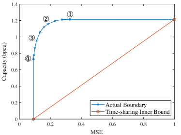
(a) The capacity-distortion boundary

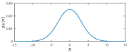
(b) $p_{\mathsfbr{X}}(X)$ at \tiny1⃝

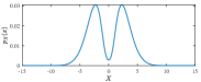
(c) $p_{\mathsfbr{X}}(X)$ at \tiny2⃝

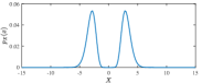
(d) $p_{\mathsfbr{X}}(X)$ at \tiny3⃝

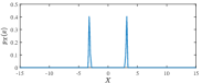
(e) $p_{\mathsfbr{X}}(X)$ at \tiny4⃝

Figure 5: The capacity-distortion boundary of the real-valued SISO Gaussian channel scenario with $B=10$dB, as well as the Pareto-optimal input distributions $p_{\mathsfbr{X}}(X)$ along the boundary.

Note that there is not enough room to accommodate ST in the SISO scenario. Therefore, the S&C tradeoff in the aforementioned example follows solely from the difference in signal preference between communication and sensing tasks. Intuitively, communication tasks would favor signals with a higher degree of randomness, in order to pack more information into the signal. For example, the capacity for AWGN channels is achieved by using Gaussian-distributed signals, where the Gaussian distribution has the maximum entropy under power constraint. By contrast, sensing tasks favor signals that are deterministic in some sense, in order to better distinguish the received signals (echoes) coupled with sensing parameters taking different values. Such a tradeoff is termed as deterministic-random tradeoff (DRT) [11].

Naturally, we would then wonder whether the DRT exists in more general scenarios, what effect it would exhibit, and how it would interact with the ST when it exists. Unfortunately, although the modified B-A algorithm is universal in principle, it is hardly applicable to the general settings in a practical sense, due to its enormous computational complexity. To elaborate, the modified B-A algorithm relies on numerical integration, which could be computationally prohibitive when the dimensionality of the signals or the sensing parameters is high. For example, if the number of samples per dimension is $K$, the total number of samples $N_{\rm MC}$ that the widely used Monte Carlo integration method would require will be on the order of $N_{\rm MC}=O\big{(}K^{N_{\bm{\mathsfbr{Y}}}+N_{\bm{\mathsfbr{X}}}+N_{\bm{\seta}}}\big{)}$, where $N_{\bm{\mathsfbr{Y}}}$, $N_{\bm{\mathsfbr{X}}}$ and $N_{\bm{\seta}}$ are the dimensionalities of $\bm{\mathsfbr{Y}}$, $\bm{\mathsfbr{X}}$, and $\bm{\seta}$, respectively. The exponentially increasing sample complexity would easily surpass the capability of most computing devices, even for small-scale MIMO systems. Furthermore, the modified B-A algorithm cannot provide analytical solutions, which can be useful for practical system design.

Considering these difficulties, to push further our understanding of the S&C tradeoff, we might need to sacrifice the generality of the capacity-distortion theory to some degree. For example, we may try and find specific distortion functions (or non-distortion sensing-induced communication costs, as implied by (13)), that are both easy to analyze and sufficiently general to reflect ST and DRT. In what follows, we shall consider one such example in detail.

IV CRB-Rate Region

We now focus our attention from the distortion measure $d(\bm{\seta},\hat{\bm{\seta}})$ to a specific sensing metric, namely, CRB for target parameter estimation. Unlike the MSE that specifically relies on the employed estimator, CRB serves as a globally lower bound for all unbiased estimators (satisfying the regularity condition), which usually leads to more tractable analytical expressions, and is achievable at high-SNR regimes [18]. Recalling the single-letterization of the expected distortion in (15), one may treat the CRB as a cost function of the transmitted codeword $\bm{\mathsfbr{X}}$, and consider the interplay between the CRB and communication rate as a special case of the C-D tradeoff.

IV-A Vector Gaussian System Model

We commence by re-examining the model in (2), which may be extended to a more generic form as

$$\bm{\mathsfbr{Y}}_{{\rm c}} =\bm{\mathsfbr{H}}_{\rm c}\bm{\mathsfbr{X}}+\bm{\mathsfbr{Z}}_{{\rm c}},$$ (18a)

$$\bm{\mathsfbr{Y}}_{{\rm s}} =\bm{\mathsfbr{H}}_{\rm s}(\bm{\seta})\bm{\mathsfbr{X}}+\bm{\mathsfbr{Z}}_{{\rm s}},$$ (18b)

where the sensing channel $\bm{\mathsfbr{H}}_{\rm s}\in\mathbb{C}^{{N_{\rm s}}\times M}$ is now defined as a deterministic, possibly nonlinear function of the sensing parameter $\bm{\seta}\in\mathbb{R}^{K}$, e.g., angular MIMO radar channel [22]. If not otherwise specified, the transmitted codeword $\bm{\mathsfbr{X}}\in\mathbb{C}^{M\times T}$ will be referred to as an ISAC signal matrix in this section. This model may be viewed as a special case of the generic model shown in Fig. 4. Following the preceding memoryless channel assumption, both the sensing parameter $\bm{\seta}$ and communication channel $\bm{\mathsfbr{H}}_{\rm c}\in\mathbb{C}^{{N_{\rm c}}\times M}$ vary every $T$ symbols in an i.i.d. manner. The discussion on channels with memory (e.g., Markov channels) are designated as our future works. For convenience, we also assume that the ISAC Tx has perfect knowledge on $\bm{\mathsfbr{H}}_{\rm c}$. Finally, $\bm{\mathsfbr{Z}}_{{\rm c}}$ and $\bm{\mathsfbr{Z}}_{{\rm s}}$ are zero-mean white Gaussian noise matrices with variances of $\sigma_{{\rm c}}^{2}$ and $\sigma_{{\rm s}}^{2}$, respectively.

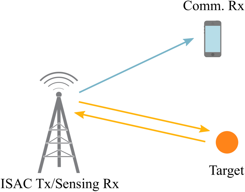
(a) Monostatic sensing

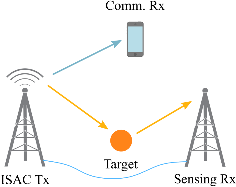
(b) Bistatic sensing

Figure 6: The ISAC scenarios described in (18), where the dual-functional waveform $\bm{\mathsfbr{X}}$ is known to both the ISAC Tx and sensing receiver (Rx).

At this point, it would be worthwhile to concretize the separate channel models in (18) by illustrating the specific scenarios concerned in this section. As shown in Fig. 6, the ISAC Tx emits a dual-functional signal $\bm{\mathsfbr{X}}$ to simultaneously communicate with a single communication Rx and sense one or more targets. The sensing Rx is either collocated with the Tx (monostatic sensing), or connected with the Tx with a wired link (bistatic sensing). In both cases, both the Tx and sensing Rx have perfect knowledge about the ISAC signal $\bm{\mathsfbr{X}}$. Nevertheless, $\bm{\mathsfbr{X}}$ is unknown to the communication Rx as it conveys useful information intended for the communication user. We are thus temped to model $\bm{\mathsfbr{X}}\sim p_{\bm{\mathsfbr{X}}}(\bm{X})$ as a random matrix, whose realization is perfectly known at both the ISAC Tx and sensing Rx, but is unknown at the communication Rx.

IV-B CRB with Random but Known Nuisance Parameters

Since the communication performance of (18a) can be directly measured by the mutual information $I(\bm{\mathsfbr{X}};\bm{\mathsfbr{Y}}_{\rm c}|\bm{\mathsfbr{H}}_{\rm c})$, we are now in a position to rethink the sensing performance evaluation in ISAC systems. Indeed, in conventional radar systems, probing signals are typically deterministic, well-designed with good ambiguity properties. In ISAC systems, on the other hand, the transmit signal randomly varies from block to block given the communication data embedded in the signal. This imposes a unique challenge in defining the CRB, which now becomes a function of the random signal $\bm{\mathsfbr{X}}$.

One possible approach would be to treat $\bm{\mathsfbr{X}}$ as a nuisance parameter, and either consider it as a part of the unknown sensing parameter, or integrate it out of the likelihood function describing the observations, leading to classical hybrid or marginal CRB expressions, respectively. Nonetheless, neither of these methods grasps the fundamental feature of the ISAC system, that the random signal $\bm{\mathsfbr{X}}$ is known to the sensing Rx, and is thus loose in general. To that end, we resort to a Miller-Chang type CRB [23] by computing the CRB for a given instance of $\bm{\mathsfbr{X}}$, and take the expectation over $\bm{\mathsfbr{X}}$. For any weakly unbiased estimator of $\bm{\seta}$, the MSE is lower bounded by the Miller-Chang Bayesian CRB in the form of

$${\rm MSE}_{\bm{\seta}}(\hat{\bm{\seta}})\geqslant\mathbb{E}\left({\rm tr}\left\{\bm{\mathsfbr{J}}_{\bm{\seta}|\bm{\mathsfbr{X}}}^{-1}\right\}\right),$$ (19)

where the expectation is taken with respect to $\bm{\mathsfbr{X}}$, and $\bm{\mathsfbr{J}}_{\bm{\seta}|\bm{\mathsfbr{X}}}$ denotes the Bayesian Fisher Information Matrix (BFIM) of $\bm{\seta}$ given by

$$\bm{\mathsfbr{J}}_{\bm{\seta}|\bm{\mathsfbr{X}}} \!:=\!\mathbb{E}\!\left\{\!\frac{\partial\ln p_{\bm{\mathsfbr{Y}}_{\rm s}|\bm{\mathsfbr{X}},\bm{\seta}}(\bm{Y}_{\rm s}|\bm{X},\bm{\eta})}{\partial\bm{\eta}}\frac{\partial\ln p_{\bm{\mathsfbr{Y}}_{\rm s}|\bm{\mathsfbr{X}},\bm{\seta}}(\bm{Y}_{\rm s}|\bm{X},\bm{\eta})}{\partial\bm{\eta}^{\rm T}}\bigg{|}\bm{\mathsfbr{X}}\right\}$$ (20)

$$\hskip 14.22636pt+\mathbb{E}\left\{\frac{\partial\ln p_{\bm{\seta}}(\bm{\eta})}{\partial\bm{\eta}}\frac{\partial\ln p_{\bm{\seta}}(\bm{\eta})}{\partial\bm{\eta}^{\rm T}}\right\}.$$

More precisely, the BFIM $\bm{\mathsfbr{J}}_{\bm{\seta}|\bm{\mathsfbr{X}}}$ can be expressed as an affine map of the sample covariance matrix $\bm{\mathsfbr{R}}_{\bm{\mathsfbr{X}}}=T^{-1}\bm{\mathsfbr{X}}\bm{\mathsfbr{X}}^{\rm H}$ [11]

$$\bm{\mathsfbr{J}}_{\bm{\seta}|\bm{\mathsfbr{X}}}=\frac{T}{\sigma_{\rm s}^{2}}\bm{\varPhi}(\bm{\mathsfbr{R}}_{\bm{\mathsfbr{X}}}),$$ (21)

where

$$\bm{\varPhi}(\bm{A})=\sum_{i=1}^{r_{1}}\widetilde{\bm{F}}_{i}\bm{A}^{\rm T}\widetilde{\bm{F}}_{i}^{\rm H}+\sum_{j=1}^{r_{2}}\widetilde{\bm{G}}_{j}\bm{A}\widetilde{\bm{G}}_{j}^{\rm H}+\widetilde{\bm{J}}_{\rm P},$$ (22)

and $\widetilde{\bm{J}}_{\rm P}=\sigma_{\rm s}^{2}T^{-1}\bm{J}_{\rm P}$, with the term $\bm{J}_{\rm P}$ being contributed by the prior distribution $p_{\bm{\seta}}(\bm{\eta})$, i.e., the second term in (20). In particular, the matrices $\widetilde{\bm{F}}_{i}$ and $\widetilde{\bm{G}}_{j}$ are partitioned from the Jacobian matrix $\bm{\mathsfbr{F}}:=\frac{\partial\operatorname{vec}(\bm{\mathsfbr{H}}_{\rm s}^{\ast})}{\partial\bm{\seta}}$.

By noting (19), it turns out that the Miller-Chang CRB is nothing but an equivalent “expected sensing distortion” discussed in Sec. III-A (though it is not a real distortion measure), and may hence be viewed as a sensing-induced cost imposed on signaling resources. Although with high dimensionality, one may still deduce useful results on the CRB-rate tradeoff by exploiting the affine structure of the BFIM, as discussed in the sequel.

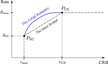
Figure 7: CRB-rate region, Pareto boundary, and time-sharing inner bound.

IV-C CRB-Rate Tradeoff

The CRB-rate tradeoff can be characterized as the following Pareto optimization problem

$$\min_{p_{\bm{\mathsfbr{X}}}(\bm{X})} \leavevmode\nobreak\ \leavevmode\nobreak\ \alpha\mathbb{E}\left({\rm tr}\left\{\left[\bm{\varPhi}({\bm{\mathsfbr{R}}}_{\bm{\mathsfbr{X}}})\right]^{-1}\right\}\right)-(1-\alpha)I(\bm{\mathsfbr{X}};\bm{\mathsfbr{Y}}_{\rm c}|\bm{\mathsfbr{H}}_{\rm c}),$$ (23a)

$${\rm s.t.} \leavevmode\nobreak\ \leavevmode\nobreak\ \mathbb{E}\left({\rm tr}\left\{{\bm{\mathsfbr{R}}}_{\bm{\mathsfbr{X}}}\right\}\right)=P_{\rm T},$$ (23b)

where $\alpha\in\left[0,1\right]$ is a weighting factor controlling the priority of S&C performance. We highlight here that by moving the CRB from (23a) to (23b), (23) may be equivalently recast as a constrained capacity characterization problem with two cost functions as in (13).

Needless to say, fully depicting the Pareto boundary of the CRB-rate region would incur unaffordable computational overheads, as one has to numerically seek for optimal $p_{\bm{\mathsfbr{X}}}(\bm{X})$ by leveraging the modified B-A algorithm discussed in Sec. III-B. To reveal fundamental insights into the CRB-rate tradeoff, we are interested in the two corner points over the Pareto frontier as shown in Fig. 7, namely, $P_{\rm CS}$, the minimum achievable sensing CRB constrained by the maximum communication capacity, and $P_{\rm SC}$, the maximum achievable rate constrained by the minimized CRB. It is obvious that the line segment linked to two points forms a time-sharing inner-bound. In what follows, we briefly characterize the S&C performance at the two points.

IV-D $P_{\rm CS}$ Performance Characterization

Let us first examine the point $P_{\rm CS}$. For point-to-point Gaussian channel, it is well-known that Gaussian distribution is the unique capacity-achieving input distribution (CAID) under an average power cost [24], in which case (23) reduces to a capacity characterization problem with only power constraint by simply letting $\alpha=0$. More specifically, at $P_{\rm CS}$, each column of $\bm{\mathsfbr{X}}$ follows a circularly symmetric complex Gaussian distribution $\mathcal{CN}(\bm{0},\widetilde{\bm{R}}_{\bm{\mathsfbr{X}}}^{\rm CS})$ in an i.i.d. manner, where the statistical covariance matrix $\widetilde{\bm{R}}_{\bm{\mathsfbr{X}}}^{\rm CS}$ is obtained by solving the following rate maximization problem

$$\begin{gathered}{R_{\rm{max}}}=\mathop{\max}\limits_{\widetilde{\bm{R}}\succcurlyeq{\bm{0}},\widetilde{\bm{R}}={\widetilde{\bm{R}}^{\rm H}}}\mathbb{E}\left\{\log\left|{{\bm{I}}+\sigma_{c}^{-2}{{\bm{\mathsfbr{H}}}_{c}}\widetilde{\bm{R}}{\bm{\mathsfbr{H}}}_{c}^{\rm H}}\right|\right\}\hfill\\ \;\;\;\;\;\;\;\;\;\;\;\;\;\;\;\;\;\;\;{\rm s.t.}\;\;\;\;\;{\rm tr}\left\{\widetilde{\bm{R}}\right\}\leqslant{P_{\rm T}}\hfill\\ \;\;\;\;\;\;\;\;\;=\mathbb{E}\left\{\log\left|{{\bm{I}}+\sigma_{\rm c}^{-2}{{\bm{\mathsfbr{H}}}_{\rm c}}\widetilde{\bm{R}}_{\bm{\mathsfbr{X}}}^{\rm CS}{\bm{\mathsfbr{H}}}_{c}^{\rm H}}\right|\right\}.\hfill\\ \end{gathered}$$ (24)

It is readily observed that the optimal solution of (24) has the following eigenvalue decomposition structure

$$\widetilde{\bm{R}}_{\bm{\mathsfbr{X}}}^{\rm CS}=\bm{U}_{\rm c}\bm{\varLambda}_{\rm c}\bm{U}_{\rm c}^{\rm H},$$ (25)

where $\bm{U}_{\rm c}$ contains the right singular vectors of ${{\bm{\mathsfbr{H}}}_{c}}$, and $\bm{\varLambda}_{\rm c}$ contains the optimal eigenvalues that can be attained from the water-filling method. Accordingly, the optimal ISAC signal structure at $P_{\rm CS}$ is

$$\bm{\mathsfbr{X}}^{\rm CS}=\bm{U}_{\rm c}\bm{\varLambda}_{\rm c}^{\frac{1}{2}}\bm{\mathsfbr{D}},$$ (26)

where the entries of $\bm{\mathsfbr{D}}$ i.i.d. subject to $\mathcal{CN}(0,1)$.

One would then raise the natural question: What is the sensing performance if a Gaussian signal is transmitted? From (19) to (22), it is obvious that the CRB is determined by the sample covariance matrix $\bm{\mathsfbr{R}}_{\bm{\mathsfbr{X}}}=T^{-1}\bm{\mathsfbr{X}}\bm{\mathsfbr{X}}^{\rm H}$ rather than the statistical covariance matrix $\widetilde{\bm{R}}_{\bm{\mathsfbr{X}}}=\mathbb{E}(\bm{\mathsfbr{R}}_{\bm{\mathsfbr{X}}})$. At $P_{\rm CS}$, since each column of $\bm{\mathsfbr{X}}$ is i.i.d. Gaussian distributed, $\bm{\mathsfbr{R}}_{\bm{\mathsfbr{X}}}$ follows a complex Wishart distribution. Note the fact that ${{\text{tr}}\left({{{\left[{{\bm{\varPhi}}\left({{\bm{\mathsfbr{R}}_{\bm{\mathsfbr{X}}}}}\right)}\right]}^{-1}}}\right)}$ is a convex function in $\bm{\mathsfbr{R}}_{\bm{\mathsfbr{X}}}$. Upon denoting the CRB at $P_{\rm CS}$ as $\epsilon_{\rm CS}$, and based on Jensen’s inequality, we have

$$\begin{gathered}{\epsilon_{{\rm{CS}}}}\triangleq\frac{T}{\sigma_{\rm s}^{2}}{\mathbb{E}}\left\{{{\text{tr}}\left({{{\left[{{\bm{\varPhi}}\left({{\bm{\mathsfbr{R}}_{\bm{\mathsfbr{X}}}}}\right)}\right]}^{-1}}}\right)}\right\}\geqslant\frac{T}{\sigma_{\rm s}^{2}}{\text{tr}}\left\{{{{\left({{\bm{\varPhi}}\left[{\mathbb{E}\left({\bm{\mathsfbr{R}}_{\bm{\mathsfbr{X}}}}\right)}\right]}\right)}^{-1}}}\right\}\hfill\\ \;\;\;\;\;\;=\frac{T}{\sigma_{\rm s}^{2}}{\text{tr}}\left\{{{{\left[{{\bm{\varPhi}}\left(\widetilde{\bm{R}}_{\bm{\mathsfbr{X}}}^{\rm CS}\right)}\right]}^{-1}}}\right\},\hfill\\ \end{gathered}$$ (27)

which holds for arbitrarily distributed $\bm{\mathsfbr{R}}_{\bm{\mathsfbr{X}}}$. This suggests there is certain performance loss for sensing due to the Wishart distributed $\bm{\mathsfbr{R}}_{\bm{\mathsfbr{X}}}$, since the Jensen lower bound is attained when $\bm{\mathsfbr{R}}_{\bm{\mathsfbr{X}}}=\mathbb{E}(\bm{\mathsfbr{R}}_{\bm{\mathsfbr{X}}})=\widetilde{\bm{R}}_{\bm{\mathsfbr{X}}}$, which holds for Wishart matrix only when $T\to\infty$.

A more non-trivial result in [11] depicts the upper bound of ${\epsilon_{{\rm{CS}}}}$, given by

$${\mathbb{E}}\left\{{{\text{tr}}\left({{{\left[{{\bm{\varPhi}}\left({{\bm{\mathsfbr{R}}_{\bm{\mathsfbr{X}}}}}\right)}\right]}^{-1}}}\right)}\right\}\leqslant\frac{T\cdot{\rm tr}\left\{\bm{\varPhi}(\widetilde{\bm{R}}_{\bm{\mathsfbr{X}}}^{\rm CS})^{-1}\right\}}{T-\min\{K,\mathsfbr{M}_{\rm CS}\}},$$ (28)

with $\mathsfbr{M}_{\rm CS}={\rm rank}(\widetilde{\bm{R}}_{\bm{\mathsfbr{X}}}^{\rm CS})$, which clearly indicates that the maximum sensing performance loss at $P_{\rm CS}$ is jointly determined by the number of sensing parameters $K$ and the rank of $\widetilde{\bm{R}}_{\bm{\mathsfbr{X}}}^{\rm CS}$. Note again that when $T\to\infty$, the sensing performance is lossless since the upper bound converges to its lower counterpart.

IV-E $P_{\rm SC}$ Performance Characterization

The performance characterization at $P_{\rm SC}$ becomes more challenging compared to that of $P_{\rm CS}$, as the achieving strategy remains unknown in general. By denoting the achievable CRB at $P_{\rm SC}$ as $\epsilon_{\min}$, and using the Jensen’s inequality again, we have

$$\begin{gathered}\frac{T}{\sigma_{\rm s}^{2}}{\mathbb{E}}\left\{{{\text{tr}}\left({{{\left[{{\bm{\varPhi}}\left({{\bm{\mathsfbr{R}}_{\bm{\mathsfbr{X}}}}}\right)}\right]}^{-1}}}\right)}\right\}\geqslant\frac{T}{\sigma_{\rm s}^{2}}{\text{tr}}\left\{{{{\left({{\bm{\varPhi}}\left[{\mathbb{E}\left({\bm{\mathsfbr{R}}_{\bm{\mathsfbr{X}}}}\right)}\right]}\right)}^{-1}}}\right\}\hfill\\ =\frac{T}{\sigma_{\rm s}^{2}}{\text{tr}}\left\{{{{\left[{{\bm{\varPhi}}\left(\widetilde{\bm{R}}_{\bm{\mathsfbr{X}}}^{\rm SC}\right)}\right]}^{-1}}}\right\}\triangleq\epsilon_{\min}\hfill\\ \end{gathered}$$ (29)

holds for any complex semidefinite matrix ${\bm{\mathsfbr{R}}_{\bm{\mathsfbr{X}}}}$ satisfying the average power constraint, where $\widetilde{\bm{R}}_{\bm{\mathsfbr{X}}}^{\rm SC}$ is the solution of the deterministic CRB minimization problem

$${{\widetilde{\bm{R}}_{\bm{\mathsfbr{X}}}^{\rm{SC}}}}=\mathop{\arg\min}\limits_{{\widetilde{\bm{R}}}\succcurlyeq{\mathbf{0}},\;{\widetilde{\bm{R}}}={{\widetilde{\bm{R}}}^{\rm H}}}\;{\text{tr}}\left\{\left[{{{\bm{\varPhi}}}\left({\widetilde{\bm{R}}}\right)}\right]^{-1}\right\}\;\;\operatorname{s.t.}\;{\text{tr}}\left({\widetilde{\bm{R}}}\right)\leqslant{P_{\rm T}}.$$ (30)

While problem (30) is a convex semidefinite programming (SDP), it is not strictly convex. As a result, the optimal solution is not unique. In fact, all the solutions of an SDP belongs to the subspace spanned by the maximum-rank solution, hence may be parameterized as

$$\widetilde{\bm{R}}_{\bm{\mathsfbr{X}}}^{\rm{SC}}=\bm{U}_{\rm s}\bm{\varLambda}_{\rm s}\bm{U}_{\rm s}^{\rm H},$$ (31)

where $\bm{U}_{\rm s}$ consists of the eigenvectors of the maximum-rank sensing-optimal solution corresponding to the non-zero eigenvalues, while $\bm{\varLambda}_{\rm s}$ is a positive semidefinite Hermitian matrix.

Provably, (30) admits an unique solution in most situations [11], where the equality in (29) holds iff

$$\bm{\mathsfbr{R}}_{\bm{\mathsfbr{X}}}=\mathbb{E}(\bm{\mathsfbr{R}}_{\bm{\mathsfbr{X}}})=\widetilde{\bm{R}}_{\bm{\mathsfbr{X}}}^{\rm{SC}}.$$ (32)

That is, the sample covariance matrix $\bm{\mathsfbr{R}}_{\bm{\mathsfbr{X}}}$ becomes a deterministic matrix when the global minimum of the CRB $\epsilon_{\min}$ is attained. One may then wonder whether there is any communication DoF left in the ISAC signal at $P_{\rm SC}$. The answer is non-trivially yes. This is because a deterministic $\bm{\mathsfbr{R}}_{\bm{\mathsfbr{X}}}$ does not necessarily imply a deterministic $\bm{\mathsfbr{X}}$. The latter may still be a random signal conveying information, given by

$$\bm{\mathsfbr{X}}^{\rm SC}=\sqrt{T}(\widetilde{\bm{R}}_{\bm{\mathsfbr{X}}}^{\rm{SC}})^{\frac{1}{2}}\bm{\mathsfbr{Q}}=\sqrt{T}\bm{U}_{\rm s}\bm{\varLambda}_{\rm s}^{\frac{1}{2}}\bm{\mathsfbr{Q}},$$ (33)

where $\bm{\mathsfbr{Q}}\in\mathbb{C}^{\mathsfbr{M}_{\rm SC}\times T}$ is a random semi-unitary matrix such that $\bm{\mathsfbr{Q}}\bm{\mathsfbr{Q}}^{\rm H}=\bm{I}$, where $\mathsfbr{M}_{\rm SC}={\rm rank}(\widetilde{\bm{R}}_{\bm{\mathsfbr{X}}}^{\rm{SC}})$. Since $(\widetilde{\bm{R}}_{\bm{\mathsfbr{X}}}^{\rm{SC}})^{\frac{1}{2}}$ is deterministic, the communication DoFs at $P_{\rm SC}$ are only contributed by the randomness of $\bm{\mathsfbr{Q}}$.

We are now ready to characterize the achievable communication rate at $P_{\rm SC}$. That is, seeking for the optimal distribution $p_{\bm{\mathsfbr{Q}}}({\bm{Q}})$ over the set of all $\mathsfbr{M}_{\rm SC}\times T$ semi-unitary matrices, namely, the Stiefel manifold $\mathcal{S}(T,\mathsfbr{M}_{\rm SC})$, such that the mutual information $I(\bm{\mathsfbr{Q}};\bm{\mathsfbr{Y}}_{\rm c}|\bm{\mathsfbr{H}}_{\rm c})$ is maximized. In the high-SNR regime, this is equivalent to solving the sphere packing problem over the Stiefel manifold, where the optimal $p_{\bm{\mathsfbr{X}}}(\bm{X})$ is uniform distribution, leading to the following asymptotic achievable rate [11]

$$R_{\rm SC}=\mathbb{E}\Big{\{}\Big{(}1-\frac{\mathsfbr{M}_{\rm SC}}{2T}\Big{)}\log|\sigma_{\rm c}^{-2}\bm{\mathsfbr{H}}_{\rm c}\widetilde{\bm{R}}_{\bm{\mathsfbr{X}}}^{\rm SC}\bm{\mathsfbr{H}}_{\rm c}^{\rm H}|+\mathsfbr{c}_{0}\Big{\}}+O(\sigma_{\rm c}^{2}),$$ (34)

where

$$\mathsfbr{c}_{0}=\frac{\mathsfbr{M}_{\rm SC}}{T}\Big{[}\Big{(}T\!-\!\frac{\mathsfbr{M}_{\rm SC}}{2}\Big{)}\log\frac{T}{e}\!-\!\log\Gamma(T)\!+\!\log(2\sqrt{\pi})\Big{]}$$ (35)

converges to zero as $T\rightarrow\infty$.

Observe immediately that when $T\rightarrow\infty$, the communication DoFs are lossless, since even a Gaussian matrix would have asymptotically orthogonal rows with the increase of $T$, making it asymptotically equivalent to a semi-unitary matrix.

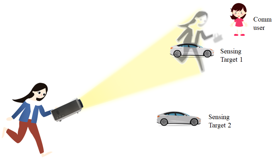
Figure 8: Graphical illustration of the projector metaphor.

IV-F The Two-fold S&C Tradeoff: A Projector Metaphor

The above results clearly demonstrate the effect of both ST and DRT in an ISAC system. By comparing the left-most parts of $\bm{\mathsfbr{X}}^{\rm CS}$ and $\bm{\mathsfbr{X}}^{\rm SC}$, we see that the communication- and sensing-optimal ISAC signals should be aligned to $\bm{U}_{\rm c}$ and $\bm{U}_{\rm s}$, respectively, which may be regarded as the orthogonal bases of communication and sensing subspaces. Then the ST is nothing but to flow the signal power from $\operatorname{span}(\bm{U}_{\rm c})$ to $\operatorname{span}(\bm{U}_{\rm s})$, perfectly fitting the picture of the “ISAC torch” metaphor. More interestingly, by comparing the right-most parts of $\bm{\mathsfbr{X}}^{\rm CS}$ and $\bm{\mathsfbr{X}}^{\rm SC}$, e.g., $\bm{\mathsfbr{D}}$ and $\bm{\mathsfbr{Q}}$, we see that communication- and sensing-optimal signals adopt Gaussian and semi-unitary codebooks, respectively, which again reflects the DRT. That is, when the ISAC system moves along the Pareto frontier from $P_{\rm CS}$ to $P_{\rm SC}$, $p_{\bm{\mathsfbr{X}}}(\bm{X})$ gradually changes from Gaussian to less random distribution, and eventually becomes uniform distribution over semi-unitary matrices. In that sense, the DRT considered in Fig. 5 is simply a one-dimensional special case, since the semi-unitary matrix reduces to constant-modulus signals in its scalar form, namely, the BPSK modulation in Fig. 5(e).

In addition to the tradeoff between input distributions, the DRT may also be observed in the attainable communication and sensing DoF at the two corner points. At $P_{\rm CS}$, the communication subsystem apparently acquires the full DoF of the Gaussian channel, namely, $\mathsfbr{M}_{\rm CS}$, which is the rank of $\widetilde{\bm{R}}_{\bm{\mathsfbr{X}}}^{\rm CS}$. As shown in (28), due to the Gaussian signaling, the sensing subsystem suffers from the DoF loss, or, equivalently, the reduction in the number of individual observations of the target, which is up to $\min\{K,\mathsfbr{M}_{\rm CS}\}$. At $P_{\rm SC}$, the sensing subsystem attains the full DoF of $T$ thanks to the deterministic signal sample covariance matrix. In contrast, the semi-unitary signaling incurs a communication DoF loss of $\frac{\mathsfbr{M}_{\rm SC}^{2}}{2T}$, as indicated by (34).

To achieve the S&C performance tradeoff, it is critical to determine the steering direction of the ISAC signal. More importantly, what kind of codebook is transmitted through that direction also matters. With the above understanding, we may now correct the “ISAC torch” metaphor with a more comprehensive picture, i.e., the “ISAC projector”. As shown in Fig. 8: A child (the ISAC Tx) holds a projector, and wishes to simultaneously illuminate a target (sensing) while sending an image to a receiver (communication). To form an image, the brightness of each pixel may be used to convey information. Nevertheless, those dark pixels result in imperfect illumination of the target.

V DRT and ST in Practical ISAC Systems

V-A DRT: Sensing with Random Signals

The lessons learned from the DRT inspired us to rethink the practical design philosophy of ISAC systems. In particular, one has to take the randomness of communication data into account while conceiving a sensing strategy, which is a unique challenge emerged in the context of ISAC. In this subsection, we investigate a novel precoding design for sensing with random signals.

Let us consider again the sensing model (18b), with the sensing parameters being the entries of the channel matrix $\bm{\mathsfbr{H}}_{\rm s}$, i.e., $\bm{\seta}=\operatorname{vec}(\bm{\mathsfbr{H}}_{\rm s})$. For a given instance of $\bm{\mathsfbr{X}}$, the linear minimum MSE (LMMSE) estimator reads

$$\hat{\bm{\mathsfbr{H}}}_{\rm{LMMSE}}=\bm{\mathsfbr{Y}}_{\rm s}\left(\bm{\mathsfbr{X}}^{\rm H}\bm{R}_{\bm{\mathsfbr{H}}}\bm{\mathsfbr{X}}+\sigma_{\rm s}^{2}N_{\rm s}\bm{I}\right)^{-1}\bm{\mathsfbr{X}}^{\rm H}\bm{R}_{\bm{\mathsfbr{H}}},$$ (36)

where $\bm{R}_{\bm{\mathsfbr{H}}}=\mathbb{E}(\bm{\mathsfbr{H}}_{\rm s}^{\rm H}\bm{\mathsfbr{H}}_{\rm s})$ represents the channel correlation matrix. The resulting estimation error is given as

$$\xi_{\bm{\mathsfbr{H}}_{\rm s}|\bm{\mathsfbr{X}}}=\operatorname{tr}\Big{[}\Big{(}\bm{R}_{\bm{\mathsfbr{H}}}^{-1}+\frac{1}{\sigma_{\rm s}^{2}N_{\rm s}}\bm{\mathsfbr{X}}\bm{\mathsfbr{X}}^{\rm H}\Big{)}^{-1}\Big{]}.$$ (37)

Once again, the estimation error relies on the instantaneous realization of the random ISAC signal $\bm{\mathsfbr{X}}$. To depict the average sensing performance, we take the expectation of (37) over $\bm{\mathsfbr{X}}$, yielding

$$\xi_{\bm{\mathsfbr{H}}_{\rm s}}=\mathbb{E}\left\{\operatorname{tr}\Big{[}\Big{(}\bm{R}_{\bm{\mathsfbr{H}}}^{-1}+\frac{1}{\sigma_{\rm s}^{2}N_{\rm s}}\bm{\mathsfbr{X}}\bm{\mathsfbr{X}}^{\rm H}\Big{)}^{-1}\Big{]}\right\}.$$ (38)

We refer the term (38) to as the ergodic LMMSE (E-LMMSE) [25], as it may be understood as a time average over different realizations of $\bm{\mathsfbr{X}}$. Obviously, it is lower-bounded by the Miller-Chang CRB in (19).

We now investigate a specific form of the ISAC signal by letting $\bm{\mathsfbr{X}}=\bm{W}\bm{\mathsfbr{S}}$, where $\bm{W}\in\mathbb{C}^{M\times M}$ is a precoding matrix, and $\bm{\mathsfbr{S}}=\left[{\bm{\mathsfbr{s}}_{1}},{\bm{\mathsfbr{s}}_{2}},\ldots,{\bm{\mathsfbr{s}}_{T}}\right]\in\mathbb{C}^{M\times T}$ contains column-wise i.i.d. data symbols, satisfying $\mathbb{E}(\bm{\mathsfbr{s}}_{i})=\bm{0}$ and $\mathbb{E}({\bm{\mathsfbr{s}}_{i}}\bm{\mathsfbr{s}}_{i}^{\rm H})=\bm{I}$. A fundamental question to ask is: What is the optimal precoder $\bm{W}$ that minimizes the E-LMMSE? In classical MIMO radar waveform design, strictly orthogonal signals are typically employed, namely, $\frac{1}{T}\bm{\mathsfbr{S}}\bm{\mathsfbr{S}}^{\rm H}=\bm{I}$, where $\bm{\mathsfbr{S}}$ is a semi-unitary matrix, corresponding to the $P_{\rm SC}$ point discussed in Sec. IV. In such a case, it is known that the LMMSE-optimal precoder has a water-filling structure given by [26]

$$\bm{W}_{\mathsf{WF}}=\sqrt{\frac{\sigma_{\rm s}^{2}{N_{\rm s}}}{T}}\bm{Q}\Big{[}\Big{(}\mu_{0}\bm{I}-\bm{\varLambda}^{-1}\Big{)}^{+}\Big{]}^{\frac{1}{2}},$$ (39)

where $\bm{Q}$ and $\bm{\varLambda}$ contain the eigenvectors and eigenvalues of $\bm{R}_{\bm{\mathsfbr{H}}}$, respectively, and $\mu_{0}$ is a constant meeting the power constraint $\|\bm{W}_{\mathsf{WF}}\|_{F}^{2}=P_{\rm T}$. However, in the ISAC scenario, the water-filling solution (39) may not be optimal due to the randomness in $\bm{\mathsfbr{S}}$. Evidently, applying the Jensen’s inequality to (38) yields

$$\xi_{\bm{\mathsfbr{H}}_{\rm s}} =\mathbb{E}\left\{\operatorname{tr}\Big{[}\Big{(}\bm{R}_{\bm{\mathsfbr{H}}}^{-1}+\frac{1}{\sigma_{\rm s}^{2}N_{\rm s}}\bm{W}\bm{\mathsfbr{S}}\bm{\mathsfbr{S}}^{\rm H}\bm{W}^{\rm H}\Big{)}^{-1}\Big{]}\right\}$$

$$\overset{(a)}{\geqslant}\mathrm{tr}\Big{[}\Big{(}\bm{R}_{H}^{-1}+\frac{1}{\sigma_{\rm s}^{2}N_{\rm s}}\mathbb{E}_{\bm{S}}\Big{\{}\bm{W}\bm{\mathsfbr{S}}\bm{\mathsfbr{S}}^{\rm H}\bm{W}^{\rm H}\Big{\}}\Big{)}^{-1}\Big{]}$$

$$\overset{(b)}{=}\mathrm{tr}\Big{[}\Big{(}\bm{R}_{H}^{-1}+\frac{T}{\sigma_{\rm s}^{2}N_{\rm s}}\bm{W}\bm{W}^{H}\Big{)}^{-1}\Big{]},$$ (40)

where (a) is due to the convexity of $\xi_{\bm{\mathsfbr{H}}_{\rm s}|\bm{\mathsfbr{X}}}$ with respect to $\bm{\mathsfbr{S}}\bm{\mathsfbr{S}}^{\rm H}$, and (b) holds from the fact $\mathbb{E}(\bm{\mathsfbr{S}}\bm{\mathsfbr{S}}^{\rm H})=T\bm{I}$. The equality in (a) holds only asymptotically for $\frac{T}{M}\to\infty$, since $\frac{1}{T}\bm{\mathsfbr{S}}\bm{\mathsfbr{S}}^{\rm H}\neq\bm{I}$ due to the i.i.d. assumption in the columns of $\bm{\mathsfbr{S}}$.

It turns out that the water-filling solution (39) minimizes the Jensen lower bound in (V-A), rather than $\xi_{\bm{\mathsfbr{H}}_{\rm s}}$ itself. Specifically, when $T$ is comparable to $M$, and when non-unitary codebooks, e.g., Gaussian codebook (where $\bm{\mathsfbr{S}}\bm{\mathsfbr{S}}^{\rm H}$ follows Wishart distribution), are employed, the orthogonality of $\bm{\mathsfbr{S}}$ breaks and the Jensen bound is no longer tight. To see this, we show an example in Fig. 9a with $M=64,N_{\rm s}=32$, where the water-filling precoder (39) is applied to both Gaussian distributed and semi-unitary data matrix. The Jensen bound (semi-unitary sensing performance) is attained when $T\geqslant 2048$. To account for the random nature of the ISAC signal, one needs to develop novel precoders that directly minimize the E-LMMSE, rather than its Jensen lower bound. Here we briefly introduce two possible methodologies, namely, data-dependent and data-independent designs, both of which yield better performance than that of the water-filling precoder [25].

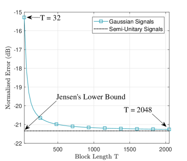
(a) $M=64,N_{\rm s}=32$

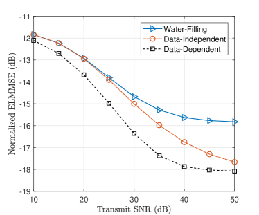
(b) $M=64,N_{\rm s}=32,T=32$

Figure 9: Sensing with random signals. (a). Tightness of the Jensen bound with an increasing block length. (b). Estimation performance of the DRT-aware precoding designs.

V-A1 Data-Dependent Precoding

Despite its randomness, the fact that $\bm{\mathsfbr{S}}$ is known at the ISAC Tx enables a precoding design based on given instances of $\bm{\mathsfbr{S}}$. Let us denote the $n$th realization of $\bm{\mathsfbr{S}}$ as $\bm{S}_{n}$, and the to-be-designed precoder as $\bm{W}_{n}$. One may then directly minimize $\xi_{\bm{\mathsfbr{H}}_{\rm s}|\bm{\mathsfbr{X}}}$ based on the known $\bm{S}_{n}$ by solving the following problem

$$\min_{\|\bm{W}_{n}\|_{F}^{2}=P_{\rm T}}\operatorname{tr}\Big{[}\Big{(}\bm{R}_{\bm{\mathsfbr{H}}}^{-1}+\frac{1}{\sigma_{\rm s}^{2}N_{\rm s}}{\bm{W}_{n}}{\bm{S}_{n}}{\bm{S}_{n}^{\rm H}}{\bm{W}_{n}^{\rm H}}\Big{)}^{-1}\Big{]}.$$ (41)

While problem (41) is non-convex, it is provable that it admits an optimal closed-form solution [27]. Consequently, one may minimize the E-LMMSE $\xi_{\bm{\mathsfbr{H}}_{\rm s}}$ by minimizing every instance of $\xi_{\bm{\mathsfbr{H}}_{\rm s}|\bm{\mathsfbr{X}}}$.

V-A2 Data-Independent Precoding

The optimality of the data-dependent precoder is achieved at the price of high complexity, as one has to solve for $\bm{W}_{n}$ for every instance $\bm{S}_{n}$. To ease the computational burden, an alternative option would be to conceive a data-independent precoder, where a single $\bm{W}$ is leveraged for every instance of $\bm{\mathsfbr{S}}$, leading to the following stochastic optimization problem

$$\min_{\|\bm{W}_{n}\|_{F}^{2}=P_{\rm T}}\mathbb{E}\left\{\operatorname{tr}\Big{[}\Big{(}\bm{R}_{\bm{\mathsfbr{H}}}^{-1}+\frac{1}{\sigma_{\rm s}^{2}N_{\rm s}}\bm{W}\bm{\mathsfbr{S}}\bm{\mathsfbr{S}}^{\rm H}\bm{W}^{\rm H}\Big{)}^{-1}\Big{]}\right\},$$ (42)

which can be solved via stochastic gradient descent (SGD) algorithm in an offline manner, where massive training data samples may be locally generated based on the adopted communication codebook.

To validate the performance of the proposed sensing precoding design for random signals, we show their corresponding estimation errors in Fig. 9b with $M=64,T=32$ and $N_{\rm s}=32$, where a Gaussian codebook is employed again for generating $\bm{\mathsfbr{S}}$. As expected, both precoding designs significantly outperform the classical water-filling approach (39). In particular, the computationally expensive data-dependent design achieves better average estimation performance (0.4-1.4 dB gain) compared to its data-independent counterpart, while the latter attains a favorable performance-complexity tradeoff. This provides strong evidence that the data randomness is non-negligible in ISAC signaling. To achieve the S&C performance boundary, DRT-aware ISAC precoding techniques are yet to be implemented in practical ISAC systems.

V-B Frequency-domain ST: Valuating Sensing Resources

Let us now turn our attention to the ST. In previous sections, we have illustrated the ST using spatial-domain examples. In these examples, roughly speaking, the ST is manifested as the preference for direct-illuminating beams, which holds for both the communication user and the sensing target. By contrast, when we consider non-spatial scenarios, the ST might take a less intuitive form, but it would also be more interesting and non-trivial.

To see this, let us consider the example of ranging waveform design, characterized by the simple observation model

$$y(t)=s(t-\tau)+n(t),$$

where $y(t)$, $s(t)$ and $n(t)$ represent the received signal, the transmitted signal, and the noise with constant power spectral density (PSD) $N_{0}$, respectively. The term $\tau=d/c$ denotes the propagation delay, with $c$ being the propagation speed, and $d$ being the distance to be estimated. For this model, the CRB reads

$$\mathbb{E}\{(d-\hat{d})^{2}\}\geqslant c^{2}(8\pi^{2}\beta^{2}{\rm SNR})^{-1},$$ (43)

where $\beta=\int_{-\infty}^{\infty}f^{2}|S(f)|^{2}{\rm d}f/\int_{-\infty}^{\infty}|S(f)|^{2}{\rm d}f$ is referred to as the “ root-mean-square (RMS) bandwidth” [28], while ${\rm SNR}=\frac{1}{N_{0}}\int_{-\infty}^{+\infty}s^{2}(t){\rm d}t$.

What does (43) imply? Upon assuming that the signal is constrained to reside in the frequency interval of $[0,f_{\rm high}]$, we find immediately that the CRB-optimal signal is in fact a sinusoidal signal with frequency $f_{\rm high}$, which maximizes the RMS bandwidth. The intuition behind this result is that, as long as the integer ambiguity can be resolved, ranging methods based on carrier phase sensing would yield the optimal performance, as has been recognized in the literature of global navigation satellite system (GNSS)-based positioning [29].

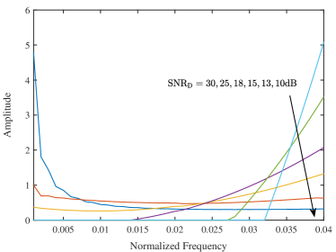
Figure 10: The PSDs of ZZB-optimal waveforms at different SNRs.

Of course, if not supplemented by further information, the integer ambiguity of a single-tone signal can never be resolved. However, CRB is known to be unable to capture the ambiguity phenomenon. To this end, we may use the Ziv-Zakai bound (ZZB) given by [30]

$$\mathbb{E}\left\{(d\!-\!\hat{d})^{2}\right\}\!\geqslant\!\int_{0}^{\epsilon_{\max}}xQ\Big{(}\sqrt{2^{-1}{\rm SNR}(1\!-\!\widetilde{R}(x))}\Big{)}{\rm d}x,$$ (44)

where $\epsilon_{\max}$ is the maximum possible ranging error, $Q(\cdot)$ denotes the Marcum Q-function, $\widetilde{R}(x)$ denotes the normalized autocorrelation function (ACF) defined as $\widetilde{R}(x)=R(x/c)/R(0)$, with $R(\tau)=\int_{-\infty}^{\infty}s(t-\tau)s(t){\rm d}t$. Although it does not admit a closed-form expression, we may observe from (44) that the ZZB can reflect the ambiguity phenomenon: It is a decreasing function with respect to $(1-\widetilde{R}(x))$. Since the normalized ACF $\widetilde{R}(x)$ achieves its maximum at $\widetilde{R}(0)=1$, $(1-\widetilde{R}(x))$ can be viewed as a measure of the sidelobe level. Intuitively, given a fixed noise level, a higher sidelobe level would make it less distinguishable from the mainlobe, and hence cause larger errors.

With the aid of ZZB, we are now able to understand the behaviour of waveforms that achieve (near-) optimal sensing performance. Numerically computed PSDs of ZZB-optimal waveforms (using the method in [30]) are plotted in Fig. 10. Observe that as the total SNR increases, the ZZB-optimal waveform would refocus its power from the low-frequency band to the high-frequency band. The reason is that when the total SNR is sufficiently high, one may effectively resolve the ambiguity caused by relatively high sidelobes, and hence the power is focused on the high-frequency band. By contrast, when the total SNR is lower, one needs to lower the sidelobe level to fight against the ambiguity issue, which would inevitably widen the mainlobe, leading to low-frequency waveforms.

(a) Communication Subspace

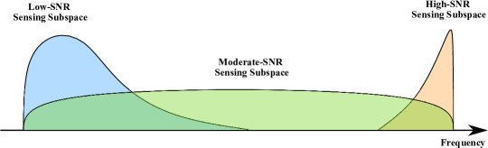
(b) Sensing Subspace

Figure 11: Frequency-domain communication and sensing subspaces (for the ranging task) in low- and high-SNR regimes.

Note that this is a remarkable observation suggesting that sensing tasks have a unique preference on the subspaces where the ISAC signal resides. This is in stark contrast to communication tasks, for which the optimal frequency-domain power allocation scheme is the water-filling strategy. In particular, the water-filling strategy assigns more power to frequency bands having higher SNR, and might even abandon some low-SNR bands when the total power constraint is stringent, or equivalently, when the total SNR is relatively low. In the language of ST, we may say that in the frequency domain, the communication subspace corresponds to those frequency bands with high SNR. By contrast, the sensing subspace is not solely dependent on the SNR; rather, as the total SNR increases, the sensing subspace would move from the low-frequency band to the high-frequency band, as portrayed in Fig. 11.

We may obtain further insights from the perspective of resource allocation. One of the resources of communication tasks is the DoF, which is manifested as the bandwidth in the frequency domain. For communication tasks, the value of the frequency bands only depends on their quality (in terms of SNR). However, for sensing tasks, the value of frequency bands depends not only on their quality, but on their location as well. In light of this, we may say that the DoF is not, in its nature, a sensing resource. We are thus motivated to ask the following question: What do we really mean when we say “sensing resources”?

VI Concluding Remarks and Open Challenges

Unfortunately, at the moment of writing, we do not have a well-stated answer to this question. After all, in contrast to communication tasks always aiming to deliver information, sensing tasks have vastly diverse purposes, and hence may rely on different resources. Apart from this question, many important problems remain open in the context of S&C tradeoffs. To name a few:

1. How does the DRT manifest itself under generic sensing performance metrics?

2. How do we characterize the S&C tradeoff when the channels are not memoryless? What are the performances of online and offline estimators in such scenarios?

3. How do we design ISAC systems that are capable of achieving the entire capacity-distortion boundary (not just the corner points)?

4. Can we unify S&C performance metrics?

These challenging questions remind us that there is still a long way to go before the merit of ISAC can be fully understood and utilized. Nevertheless, the ST-DRT decomposition (i.e. the “projector metaphor”) is likely to be a useful meta-intuition in future investigations of ISAC systems: the fundamental tradeoff in ISAC is manifested as the preference discrepancies between S&C tasks, concerning both the resources (ST) and the signal patterns (DRT).

References

- [1] ITU-R WP5D, “Draft New Recommendation ITU-R M. [IMT.FRAMEWORK FOR 2030 AND BEYOND],” 2023.
- [2] A. Hassanien, M. G. Amin, E. Aboutanios, and B. Himed, “Dual-function radar communication systems: A solution to the spectrum congestion problem,” IEEE Signal Process. Mag., vol. 36, no. 5, pp. 115–126, 2019.
- [3] C. Sturm and W. Wiesbeck, “Waveform design and signal processing aspects for fusion of wireless communications and radar sensing,” Proc. IEEE, vol. 99, no. 7, pp. 1236–1259, Jul. 2011.
- [4] Y. Cui, F. Liu, X. Jing, and J. Mu, “Integrating sensing and communications for ubiquitous IoT: Applications, trends, and challenges,” IEEE Network, vol. 35, no. 5, pp. 158–167, Sep. 2021.
- [5] F. Liu, Y.-F. Liu, A. Li, C. Masouros, and Y. C. Eldar, “Cramér-Rao bound optimization for joint radar-communication beamforming,” IEEE Trans. Signal Process., vol. 70, pp. 240–253, 2022.
- [6] D. W. Bliss, “Cooperative radar and communications signaling: The estimation and information theory odd couple,” in Proc. 2014 IEEE Radar Conf., Covington, KY, USA, May 2014, pp. 0050–0055.
- [7] D. Guo, S. Shamai, and S. Verdu, “Mutual information and minimum mean-square error in Gaussian channels,” IEEE Trans. Inf. Theory, vol. 51, no. 4, pp. 1261–1282, Apr. 2005.
- [8] M. Kobayashi, G. Caire, and G. Kramer, “Joint state sensing and communication: Optimal tradeoff for a memoryless case,” in Proc. 2018 IEEE Int. Symp. Inf. Theory (ISIT), Vail, CO, USA, Jun. 2018, pp. 111–115.
- [9] M. Kobayashi, H. Hamad, G. Kramer, and G. Caire, “Joint state sensing and communication over memoryless multiple access channels,” in Proc. 2019 IEEE Int. Symp. Inf. Theory (ISIT), Paris, France, Jul. 2019, pp. 270–274.
- [10] M. Ahmadipour, M. Kobayashi, M. Wigger, and G. Caire, “An information-theoretic approach to joint sensing and communication,” IEEE Trans. Inf. Theory, pp. 1–1, early access, 2022.
- [11] Y. Xiong, F. Liu, Y. Cui, W. Yuan, T. X. Han, and G. Caire, “On the fundamental tradeoff of integrated sensing and communications under Gaussian channels,” IEEE Trans. Inf. Theory, vol. 69, no. 9, pp. 5723–5751, 2023.
- [12] H. Joudeh, “Joint communication and target detection with multiple antennas,” in Proc. 26th International ITG Workshop on Smart Antennas and 13th Conference on Systems, Communications, and Coding (WSA & SCC 2023), Braunschweig, Germany, 2023, pp. 1–6.
- [13] H. Hua, T. X. Han, and J. Xu, “MIMO integrated sensing and communication: CRB-rate tradeoff,” IEEE Trans. Wireless Commun., pp. 1–1, early access, 2023.
- [14] M. Bică and V. Koivunen, “Radar waveform optimization for target parameter estimation in cooperative radar-communications systems,” IEEE Trans. Aerosp. Electron. Syst., vol. 55, no. 5, pp. 2314–2326, 2019.
- [15] H. Joudeh and F. M. J. Willems, “Joint communication and binary state detection,” IEEE J. Sel. Areas Inf. Theory, vol. 3, no. 1, pp. 113–124, 2022.
- [16] T. M. Cover, Elements of Information Theory, 2nd ed. John Wiley & Sons, 2006.
- [17] C. E. Shannon, “Coding theorems for a discrete source with a fidelity criterion,” IRE Int. Conv. Rec., vol. 7, no. 4, pp. 142–163, 1993.
- [18] S. M. Kay, Fundamentals of Statistical Signal Processing. Englewood Cliffs, NJ, USA: Prentice Hall, 1998.
- [19] S. Li and G. Caire, “On the capacity and state estimation error of “beam-pointing” channels: The binary case,” IEEE Trans. Inf. Theory, vol. 69, no. 9, pp. 5752–5770, Sep. 2023.
- [20] A. El Gamal and Y.-H. Kim, Network Information Theory, 1st ed. Cambridge university press, 2011.
- [21] R. Blahut, “Computation of channel capacity and rate-distortion functions,” IEEE Trans. Inf. Theory, vol. 18, no. 4, pp. 460–473, 1972.
- [22] J. Li and P. Stoica, “MIMO radar with colocated antennas,” IEEE Signal Process. Mag., vol. 24, no. 5, pp. 106–114, 2007.
- [23] R. Miller and C. Chang, “A modified Cramér-Rao bound and its applications (corresp.),” IEEE Trans. Inf. Theory, vol. 24, no. 3, pp. 398–400, May 1978.
- [24] Y. Polyanskiy and Y. Wu, Information Theory: From Coding to Learning, 1st ed. Cambridge University Press, 2023.
- [25] S. Lu, F. Liu, F. Dong, Y. Xiong, J. Xu, and Y.-F. Liu. (2023) “Sensing with random signals”. [Online]. Available: https://arxiv.org/abs/2309.02375
- [26] Y. Yang and R. S. Blum, “MIMO radar waveform design based on mutual information and minimum mean-square error estimation,” IEEE Trans. Aerosp. Electron. Syst., vol. 43, no. 1, pp. 330–343, 2007.
- [27] B. Tang, J. Tang, and Y. Peng, “MIMO radar waveform design in colored noise based on information theory,” IEEE Trans. Signal Process., vol. 58, no. 9, pp. 4684–4697, 2010.
- [28] A. Liu et al., “A survey on fundamental limits of integrated sensing and communication,” IEEE Commun. Surv. Tuts., vol. 24, no. 2, pp. 994–1034, 2022.
- [29] J. Zidan et al., “GNSS vulnerabilities and existing solutions: A review of the literature,” IEEE Access, vol. 9, pp. 153 960–153 976, 2021.
- [30] Y. Xiong and F. Liu, “SNR-adaptive ranging waveform design based on Ziv-Zakai bound optimization,” IEEE Signal Process. Lett., early access, 2023.