AugUndo: Scaling Up Augmentations for Unsupervised Depth Completion

Abstract

Unsupervised depth completion methods are trained by minimizing sparse depth and image reconstruction error. Block artifacts from resampling, intensity saturation, and occlusions are amongst the many undesirable by-products of common data augmentation schemes that affect image reconstruction quality, and thus the training signal. Hence, typical augmentations on images viewed as essential to training pipelines in other vision tasks have seen limited use beyond small image intensity changes and flipping. The sparse depth modality have seen even less as intensity transformations alter the scale of the 3D scene, and geometric transformations may decimate the sparse points during resampling. We propose a method that unlocks a wide range of previously-infeasible geometric augmentations for unsupervised depth completion. This is achieved by reversing, or “undo”-ing, geometric transformations to the coordinates of the output depth, warping the depth map back to the original reference frame. This enables computing the reconstruction losses using the original images and sparse depth maps, eliminating the pitfalls of naive loss computation on the augmented inputs. This simple yet effective strategy allows us to scale up augmentations to boost performance. We demonstrate our method on indoor (VOID) and outdoor (KITTI) datasets where we improve upon three existing methods by an average of 11.75% across both datasets.

1 Introduction

Data augmentation plays a crucial role in easing the demand for training data as it enriches the training dataset by orders of magnitude, boosting performance on various deep learning tasks [29, 35, 38], particularly by preventing overfitting. Typically, the choice of augmentation is largely task-dependent. One common axiom of choosing augmentations is that the task output should remain invariant to the augmentation. For example, image flips are viable augmentations for classifying animals, since they do not alter the resulting image label. Conversely, flipping road signs can alter their meanings; hence, such augmentations can be detrimental to tasks involving road sign recognition. For geometric tasks (i.e. depth estimation), the range of augmentations is more restricted: Stereo assumes pairs of rectified images; hence, in-plane rotations are not feasible. Image-guided sparse depth completion relies on sparse points to ground estimates to metric scale; therefore, intensity transformations on sparse depth maps that alter the scale of the 3-dimensional (3D) scene are infeasible – leaving few augmentations viable. Unsupervised learning of depth completion further limits the use of augmentations as the supervision signal comes from reconstructing the inputs, where augmenting the input introduces artifacts that impact reconstruction quality and therefore the supervision. While simulating nuisances, i.e., camera motion and orientation, is desirable, naively applying augmentations pertaining to them may do more harm than good; therefore, it is unsurprising that existing works [27, 24, 34, 42, 43, 44, 41, 46] primarily rely on a small range of photometric augmentations and flipping.

Nevertheless, photometric augmentations help model the diverse range of illumination conditions and colors of objects that may populate the scene; geometric augmentations can simulate the various camera motion, i.e. image translations can approximate small baseline movements, and scene arrangements, i.e. image flipping. But block artifacts, loss during resampling, intensity saturation are just some of the many undesirable side-effects of traditional augmentations to the image and sparse depth map. To exploit the immense amount of data derived from augmentations, we propose to simply compute the typical reconstruction loss on the original input image and sparse depth map, which bypasses negative effects of reconstruction artifacts due to photometric and geometric augmentations. However, there exists a mis-alignment between the original input (image and sparse depth), and the model depth estimate as geometric augmentations induces a change in coordinates. Hence, we undo the geometric augmentations by inverting them in the output space to align the model estimate with the training target.

Amongst the the many geometric tasks, we focus on unsupervised depth completion, the task of inferring a dense depth map from a single image and its associated sparse depth map, where augmentations have seen limited use. Here, a training sample includes the input sparse depth map, its associated image as well as additional images of neighboring views from the same 3D scene. Augmentations have traditionally been restricted to a limited range of photometric transformations and flipping – due to the need to preserve photometric consistency across a sequence of video frames used during training, and the sparse set of 3D points projected onto the image frame as a 2.5D range map; degradation to either modalities directly impacts the supervision signal. By using our method, loss functions involving sparse depth and image reconstruction from other views can be computed on the original inputs while applying augmentations that were previously not viable for the task. Our hypothesis: By “undo-ing” the augmentations, one can expand the viable set and scale up their use in training, leading to improved model performance and generalizability.

To this end, we introduce AugUndo, an augmentation framework that allows one to apply a wide range of photometric and geometric transformations on the inputs, and to “undo” them during loss computation. This allows one to compute an unsupervised loss on the original images and sparse depth maps, free of artifacts, through a warping of the output depth map – obtained from augmented input – onto the input frame of reference based on the inverse geometric transformation. In addition to group transformations that allow for output alignment, we combine them with commonly employed photometric augmentations. Lastly, we study whether non-group transformations, such as occlusion, can further improve model performance. We demonstrate AugUndo on three recent unsupervised depth completion methods and evaluate them on indoor and outdoor settings, where we improve by an average of 11.75% across all methods and datasets.

Our contributions are as follows: (i) We propose AugUndo, a simple-yet-effective framework to scale up photometric and geometric augmentations for unsupervised depth completion; AugUndo can be applied in a plug-and-play manner to existing methods with negligible increase in computational costs during training. (ii) We provide a comprehensive study ablating over combinations of eleven types of augmentations, including ones that have not been explored by existing unsupervised methods, for three different models across two datasets. We found a consistent set of augmentations that provides performance benefits for all tested models and are applicable for both indoor and outdoor scenarios. (iii) We show that AugUndo can consistently improve model performance, robustness to shifts in sparse point densities as well as zero-shot generalization; thus, validating our hypothesis.

2 Related Work

Data augmentation for depth completion. There exists extensive literature on depth completion, we highlight some of the representative work. While it is natural to apply photometric transformations, such as color jitter, in unsupervised depth completion [27, 43, 44, 42], with the exception of flipping, geometric data augmentation is less adopted and mostly applied to supervised training. For example, [1, 2, 28, 47, 40] used random scaling, translation, in-plane rotation for supervised depth completion. However, many of the the supervised methods [6, 15, 16, 22, 23, 18, 20, 30, 32, 31, 50, 46, 45, 49] also limited their augmentations to color jitter and horizontal flips – this is largely because rotation and scaling would decimate the sparse depth maps, causing points to be interpolated away. Nonetheless, for supervised methods, it is straightforward to directly apply the same transformation to the ground truth; we posit that artifacts caused from transformation of a piece-wise smooth depth map are less severe than those of an RGB image and its intensities. These artifacts would in turn affect the training signal, which relies on photometric correspondences and observed sparse points, for unsupervised methods. In contrast, our approach enables diverse geometric augmentations to be applied in a plug-and-play fashion.

Unsupervised depth completion assumes stereo images or monocular videos to be available during training. Both stereo [34, 46] and monocular [27, 43, 44, 42] training paradigms leverage photometric reprojection error as a training signal by minimizing photometric discrepancies between the input image and its reconstruction from other views. In addition to the photometric reconstruction term, previous works also minimize the difference between the input sparse depth map and the predicted depth (where sparse depth points are available) and a local smoothness regularizer. [27] used Perspective-n-Point [21] and RANSAC [8] to align consecutive video frames. [46] learned a depth prior conditioned on the image by pretraining a separate network on ground truth from an additional dataset. [25] also used synthetic data, but applied image translation to obtain ground truth in the real domain. [42] used synthetic data to learn a prior on the shapes populating a scene. [44] proposed an adaptive optimization scheme to reduce penalties incurred on occluded regions. [41] proposed a calibrated back-projection network that introduces an architectural inductive bias by mapping the image onto the 3D scene. [17] used line feature from visual SLAM and [24] introduced monitored distillation for positive congruent predictions. Amongst all of the methods discussed, augmentations are limited to a small range of photometric perturbations and image flipping because operations such as cropping reduces co-visible regions while others that require interpolation (e.g. rotation, resizing) create artifacts, which affects the reconstruction quality and cause performance degradation. Loss in sparse depth maps is further exacerbated as resampling and interpolation may cause loss of sparse points. Contrary to their augmentation schemes, our work allows for a large range of photometric and geometric augmentations to be introduced during training.

3 Method Formulation

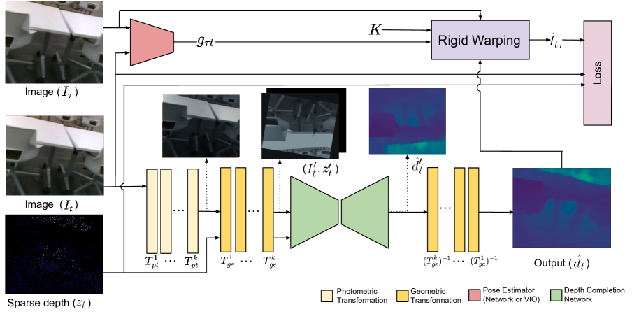
Figure 1: Overview. We augment the input images with photometric and then geometric transformations, and augment the input sparse depth with the same set of geometric transformations. Inverse geometric transformations are applied to the output depth to return it to the original reference frame by inverse warping. This enables image and sparse depth reconstruction losses to be computed using the original image and sparse depth maps, and minimizes artifacts that have limited the use of extensive augmentations in existing works.

Let $I:\Omega\subset\mathbb{R}^{2}\rightarrow\mathbb{R}^{3}_{+}$ be an RGB image that is taken by a calibrated camera. Additionally, paired with each image is a sparse point cloud projected onto the image plane (depth map) $z:\Omega_{z}\subset\Omega\rightarrow\mathbb{R}_{+}$. Let $K\in\mathbb{R}^{3\times 3}$ be the intrinsic calibration matrix , either given or estimated. Given an image and its associated sparse depth map, depth completion aims to learn a function $f_{\theta}(I,z)$ that recovers the distance between the camera to points in the 3D scene, which has been projected to the image domain $\Omega$, as a depth map. For the ease of notation, we denote the output depth map as $\hat{d}\in\mathbb{R}_{+}^{H\times W}$ where $H$ and $W$ are its height and width.

Unsupervised depth completion relies on photometric (image) and sparse depth reconstruction errors as the primary supervision signal. To this end, we assume an input of $(I_{t},z_{t})$ for an RGB image and associated sparse depth map captured at time $t$ and during training, an additional set of temporally adjacent images $I_{\tau}$ for $\tau\in\Upsilon\doteq\{t-1,t+1\}$. The reconstruction $\hat{I}_{t\tau}$ of $I_{t}$ from another image $I_{\tau}$ is given by the reprojection based on estimated depth at $\hat{d}_{t}:=f_{\theta}(\cdot)$

$$\hat{I}_{t\tau}(x)=I_{\tau}(\pi g_{\tau t}K^{-1}\bar{x}\hat{d}_{t}(x))$$ (1)

where $f_{\theta}$ denotes a depth completion network that takes both image and sparse depth map $(I_{t},z_{t})$ as input; $\bar{x}=[x^{\top},1]^{\top}$ are the homogeneous coordinates of $x\in\Omega$, $g_{\tau t}\in SE(3)$ is the relative pose (rotation and translation) of the camera from time $t$ to $\tau$, $K$ the intrinsic calibration matrix, and $\pi$ is a canonical perspective projection.

Using Eqn. 1, a depth completion network $f_{\theta}$ minimizes

$$\operatorname*{arg\,min}_{\theta} \sum_{\tau\in\Upsilon}\sum_{x\in\Omega}\alpha\rho\big{(}\hat{I}_{t\tau}(x),I_{t}(x)\big{)}+$$

$$\sum_{x\in\Omega_{z}}\beta\psi\big{(}\hat{d}_{t}(x),z_{t}(x)\big{)}+\lambda R(\hat{d_{t}})$$ (2)

where $\rho$ denotes the photometric reconstruction error, typically $L_{1}$ difference in pixel values and/or structural similarity (SSIM), $\psi$ the sparse depth reconstruction error, typically $L_{1}$ or $L_{2}$, $R$ the regularizer that biases the depth map to be piece-wise smooth with depth discontinuities aligned with edges in the image (commonly used by previous works [27, 42, 43, 41]), and $\alpha$, $\beta$ and $\lambda$ their respective weighting.

Inverse transformation. Let $\mathcal{A}_{pt}$ be the set of possible photometric transformations, and $\mathcal{A}_{ge}$ be the set of all geometric transformations. Given $\ T_{ge}\in\mathcal{A}_{ge}$, we wish to obtain an inverse transformation $T_{ge}^{-1}$ such that $T_{ge}\circ T_{ge}^{-1}\approx Id$ the identity function (note that not all transformations are bijective, for instance image rescaling, hence strict equality is not always possible). We provide several examples in Sec. 4. At each time step, we can sample a sequence of transformations $\{T_{pt}^{1}\ldots T_{pt}^{k}\}$ and $\{T_{ge}^{1}\ldots T_{ge}^{m}\}$ respectively from $\mathcal{A}_{pt}$ and $\mathcal{A}_{ge}$ to construct transformations $T_{pt}=T_{pt}^{1}\circ\cdots\circ T_{pt}^{k}$ and $T_{ge}=T_{ge}^{1}\circ\cdots\circ T_{ge}^{m}$. We denote the composition of a collection of augmentation transformations by $T=T_{ge}\circ T_{pt}$ where $T_{pt}$ denotes photometric transformation, and $T_{ge}$ denotes geometric transformation. Furthermore, we denote the inverse geometric transformations by $T_{ge}^{-1}=({T_{ge}^{m}})^{-1}\circ(T_{ge}^{m-1})^{-1}\circ\cdots\circ({T_{ge}^{1}})^{-1}$, which operates on the space of depth maps to reverse the geometric transformation so that we can warp the output depth map onto the reference frame of the original image. In practice, some of the transformations cause border regions of the image to be warped out of frame, i.e. translated off the image plane or cropped away, making them unrecoverable. Hence, after warping our output depth map back using the inverse geometric transformations, border extensions (edge paddings) are introduced to handle out-of-frame regions.

AugUndo. We perform each geometric transformation over the coordinates of the image and resample:

$$\begin{bmatrix}x^{\prime}&1\end{bmatrix}^{\top} =T_{ge}\begin{bmatrix}x&1\end{bmatrix}^{\top}$$ (3)

$$I^{\prime}(x^{\prime}) =T_{pt}(I)(x);\ z^{\prime}(x^{\prime})=z(x)\vspace{-0.5em}$$ (4)

where $T_{ge}$ is the geometric transformation, $x\in\Omega$ and $x^{\prime}\in\Omega$ are coordinates in the image grid, and $I^{\prime}$ is the image after the transformation; for ease of notation, we hereafter denote $I^{\prime}=T(I)=T_{ge}\circ T_{pt}(I)$ to include both augmentations through composition. Note that $x$ is in the original image reference frame and $x^{\prime}$ is in the transformed image reference frame. Naturally, this process can be extended to multiple geometric transformations by composing them i.e. $T_{ge}=T^{1}_{ge}\circ T^{2}_{ge}\circ\cdots\circ T^{m}_{ge}$. The reverse process is simply inverting the transformations where $T^{-1}_{ge}=(T^{m}_{ge})^{-1}\circ(T^{m-1}_{ge})^{-1}\circ\cdots\circ(T^{1}_{ge})^{-1}$:

$$\begin{bmatrix}x^{\prime\prime}&1\end{bmatrix}^{\top} =T^{-1}_{ge}\begin{bmatrix}x^{\prime}&1\end{bmatrix}^{\top}$$ (5)

$$\hat{d}(x^{\prime\prime}) =\hat{d}^{\prime}(x^{\prime})$$ (6)

where $\hat{d}^{\prime}$ is the depth map inferred from augmented inputs $(I^{\prime},z^{\prime})$. Once reverted back to the original reference frame, $\hat{d}$ is used to reconstruct $I_{t}$ from $I_{\tau}$ for $\tau\in\Upsilon$ in Eqn. 1. More details can be found in Table 1 in the Supp. Mat.

By modeling $T^{-1}_{ge}$, Eqn. 3-6 allow us to apply a wide range of augmentations, while still establishing the correspondence between $I_{t}$ and $I_{\tau}$. Specifically, for minimizing the loss function (Eqn. 2), one may simply augment the input image by $T$ and feed the augmented image and sparse depth $(I^{\prime}_{t},z^{\prime}_{t})$ to the depth completion network as input while reconstructing the original image and sparse depth $(I_{t},z_{t})$ from other views $I_{\tau}$ and the aligned output depth $\hat{d}$ (Eqn. 6). We note that the inverse transformation is critical for enabling the sparse depth reconstruction term to be computed properly in Eqn. 2; if computed in the transformed reference frame i.e. on $z^{\prime}_{t}$, many of the sparse points would be decimated by interpolation during rotation and resizing (downsampling) augmentations – leaving a lack of supervision on sparse depth in the loss function. We also note that the original image sequence is fed to the pose estimator, rather than the augmented images. This is to ensure that the estimated relative pose between the frames used during reprojection corresponds to transformation between them.

4 Augmentations

Our augmentations are selected based on nuisance variabilities often observed in the wild including changes in illumination, occlusions, and object color, and camera parameters (resize), motion (translation) and orientation (rotation).

Photometric. We include brightness, contrast, saturation, and hue, where all follow standard augmentation pipeline in existing works [27, 42, 41]. Applying the inverse of photometric augmentation can be viewed as recovering the original image; hence, we directly use original image instead of applying transformations to the intensities (which are not recoverable if saturated at the max value).

Occlusion. We consider image patch removal and sparse point removal. For image patch removal, we randomly select a percentage of pixels $x\in\Omega$ in the image and remove an arbitrary-sized patch around it by setting the corresponding region within the image to 0. For sparse point removal, we randomly sample a percentage of points $x\in\Omega_{z}$ in the sparse depth map and set them to 0. Note: we are the first to use and explore photometric occlusion augmentation in unsupervised depth completion. The inverse transformation of this is simply the original image and sparse depth map before augmentation, both used in loss computation.

Flip. We consider horizontal and vertical flips. When applied, the same flip operation are used for both input image and sparse depth maps. We record the flip type during data augmentation. During loss computation, we flip the output depth to align with the original image and sparse depth map.

Resize. We define a new image plane of the same dimensions as the input and generate a random scaling factor to be applied along both height and width directions. The image is warped to the new image plane, where any point warped out of the plane is excluded; borders of the warped image are extended to the bounds of the image plane by edge replication. Note: sparse points occupying multiple pixels are eroded to a single point for resizing with a factor greater than 1. We record the scaling factors during augmentations. During loss computation, we warp the output depth map onto a new image plane of the same dimensions by the inverse scaling matrix of the recorded scaling factors; borders of the warped depth map are extended to the bounds of the image plane by edge replication. Note: we consider resize factors greater and less than 1 as separate augmentations to study their individual contributions.

Rotation. A naive implementation of random rotation leads to loss of large areas of the image, i.e., cropped away to retain the same-size image. This discards large portions of possible co-visible regions and also supervisory signal. To preserve the entire image, we first randomly generate an angle of rotation, define a new (larger) image plane, and then resample the image based on the rotated coordinates such that the rotated image fits tightly within the new image. As image sizes within a batch can vary depending on the rotation angle, we center-pad (uniformly on each side) each image in the batch to the maximum width and height of the augmented batch so that one can construct a batch with the same image dimension. To reverse the rotation on the output depth, we warp the output depth map back by the inverse rotation matrix using the recorded the angle during augmentation. We perform a center crop on the depth map to align with the original image and sparse depth map.

Translation. We define a new image plane of the same dimensions as the input and generate random height and width translation factors. The coordinates of the input are translated and its pixels are inverse warped onto the new image plane. Any pixel warped out of the image plane is excluded. Borders of the warped image are extended to the bounds of the image plane by edge replication. We record the translation factors during data augmentations; during loss computation, we warp the output depth map onto a new image plane of the same dimensions by the inverse translation matrix and borders of the warped depth map are extended to the bounds of the image plane by edge replication.

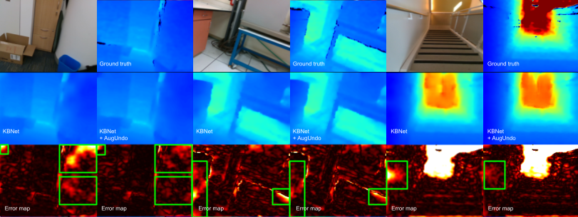
Figure 2: Qualitative comparisons on VOID. We compare KBNet trained using standard augmentations and KBNet trained with AugUndo. AugUndo consistently produces lower errors with reduced border artifacts and improves on homogeneous regions i.e., pillar (left), cabinet (middle), wall of staircase (right). See highlighted regions in error maps (last row) for detailed comparison.

Method	MAE $\downarrow$	RMSE $\downarrow$	iMAE $\downarrow$	iRMSE $\downarrow$	MAE $\downarrow$	RMSE $\downarrow$	iMAE $\downarrow$	iRMSE $\downarrow$
Dataset	VOID1500				VOID500
VOICED	74.78$\pm$2.69	139.75$\pm$4.57	39.20$\pm$1.46	71.98$\pm$2.54	137.01$\pm$4.23	235.80$\pm$7.82	71.36$\pm$1.86	130.63$\pm$5.66
+ AugUndo	52.73$\pm$0.41	111.09$\pm$0.92	26.93$\pm$0.54	54.46$\pm$0.38	92.99$\pm$1.11	176.94$\pm$1.38	46.43$\pm$0.85	91.10$\pm$1.64
FusionNet	52.11$\pm$0.44	113.30$\pm$1.18	28.53$\pm$0.52	58.79$\pm$2.01	97.73$\pm$0.73	194.32$\pm$1.36	58.65$\pm$1.31	122.95$\pm$3.04
+ AugUndo	41.16$\pm$0.18	99.21$\pm$0.39	22.23$\pm$0.35	53.07$\pm$1.30	74.97$\pm$0.69	162.71$\pm$2.39	40.44$\pm$1.39	92.11$\pm$5.79
KBNet	38.11$\pm$0.77	95.22$\pm$1.72	19.51$\pm$0.14	46.70$\pm$0.48	78.44$\pm$1.39	178.17$\pm$3.27	37.56$\pm$0.61	83.43$\pm$1.89
+ AugUndo	33.32$\pm$0.18	85.67$\pm$0.39	16.61$\pm$0.29	41.24$\pm$0.60	66.97$\pm$0.81	151.55$\pm$2.03	31.63$\pm$0.53	71.90$\pm$0.82

Table 1: Quantitative results of depth completion on VOID. Training with AugUndo improves performance by an average of 18.3% across all methods and evaluation metrics on VOID1500. When models trained on VOID1500 are tested VOID500 (fewer sparse points), AugUndo improves by 23.1%, in part due to translation, resizing and occlusion augmentations that remove sparse points from the input.

Dataset	Method	MAE $\downarrow$	RMSE $\downarrow$	iMAE $\downarrow$	iRMSE $\downarrow$
NYUv2	VOICED	2240.15$\pm$143.90	2427.91$\pm$143.49	211.41$\pm$9.60	238.99$\pm$10.89
	+ AugUndo	990.63$\pm$82.48	1181.69$\pm$65.55	110.05$\pm$6.11	132.18$\pm$6.01
	FusionNet	132.24$\pm$2.12	236.16$\pm$4.59	28.68$\pm$0.42	61.87$\pm$1.20
	+ AugUndo	124.93$\pm$3.05	227.23$\pm$4.96	25.70$\pm$0.41	54.09$\pm$0.87
	KBNet	138.31$\pm$5.74	257.99$\pm$10.36	25.48$\pm$0.63	51.77$\pm$0.99
	+ AugUndo	118.60$\pm$3.44	231.13$\pm$8.85	22.06$\pm$0.31	47.07$\pm$0.70
ScanNet	VOICED	1562.99$\pm$136.79	1764.33$\pm$146.39	270.02$\pm$17.25	311.02$\pm$17.36
	+ AugUndo	638.94$\pm$44.74	791.29$\pm$79.48	131.90$\pm$7.68	170.37$\pm$6.32
	FusionNet	109.47$\pm$3.01	206.33$\pm$6.11	55.45$\pm$1.56	122.52$\pm$2.04
	+ AugUndo	100.64$\pm$2.31	195.85$\pm$5.85	45.98$\pm$0.78	99.90$\pm$5.00
	KBNet	103.05$\pm$4.99	217.12$\pm$13.35	36.23$\pm$1.12	76.55$\pm$2.90
	+ AugUndo	82.53$\pm$4.33	175.30$\pm$11.13	29.87$\pm$1.06	63.78$\pm$1.30

Table 2: Quantitative results of zero-shot transfer from VOID to NYUv2 and ScanNet. AugUndo improves generalization of models trained on VOID to novel datasets such as NYUv2and ScanNet by an average of 25.4% for all evaluation metrics across both datasets.

Augmentation settings

Evaluation metrics

BRI

CON

SAT

HUE

FLP

TRN

ROT

RZD

RZU

RMP

RMI

MAE

RMSE

iMAE

iRMSE

✓

✓

✓

✓

✓

✓

✓

✓

✓

✓

✓

33.32$\pm$0.18

85.67$\pm$0.39

16.61$\pm$0.29

41.24$\pm$0.60

✓

✓

✓

✓

✓

38.11$\pm$0.77

95.22$\pm$1.72

19.51$\pm$0.14

46.70$\pm$0.48

✓

✓

✓

✓

✓

✓

✓

✓

✓

✓

33.46$\pm$0.27

86.02$\pm$0.69

16.84$\pm$0.22

41.78$\pm$0.63

✓

✓

✓

✓

✓

✓

✓

✓

✓

✓

33.79$\pm$0.09

86.38$\pm$0.36

17.12$\pm$0.19

42.12$\pm$0.54

✓

✓

✓

✓

✓

✓

✓

✓

✓

✓

33.73$\pm$0.30

85.84$\pm$0.22

17.05$\pm$0.16

41.73$\pm$0.47

✓

✓

✓

✓

✓

✓

✓

✓

✓

✓

33.60$\pm$0.16

86.47$\pm$0.69

16.95$\pm$0.27

41.65$\pm$0.44

✓

✓

✓

✓

✓

✓

✓

34.14$\pm$0.37

87.26$\pm$0.74

17.09$\pm$0.17

42.57$\pm$1.33

✓

✓

✓

✓

✓

✓

✓

✓

✓

✓

44.38$\pm$0.89

106.87$\pm$0.89

22.91$\pm$0.68

52.55$\pm$0.57

✓

✓

✓

✓

✓

✓

✓

✓

✓

✓

33.92$\pm$0.19

87.19$\pm$0.55

17.09$\pm$0.03

42.23$\pm$0.23

✓

✓

✓

✓

✓

✓

✓

✓

✓

✓

33.68$\pm$0.19

85.86$\pm$0.51

16.92$\pm$0.03

41.47$\pm$0.18

✓

✓

✓

✓

✓

✓

✓

✓

✓

✓

35.77$\pm$0.43

89.88$\pm$0.84

17.81$\pm$0.23

42.75$\pm$0.38

✓

✓

✓

✓

✓

✓

✓

✓

✓

✓

35.69$\pm$0.25

90.40$\pm$0.71

17.75$\pm$0.12

42.82$\pm$0.20

✓

✓

✓

✓

✓

✓

✓

✓

✓

✓

37.73$\pm$0.27

92.62$\pm$0.20

19.44$\pm$0.18

45.47$\pm$0.37

✓

✓

✓

✓

✓

✓

✓

✓

✓

✓

33.64$\pm$0.22

86.26$\pm$0.23

16.80$\pm$0.13

41.60$\pm$0.64

Table 3: Ablation study for KBNet on VOID dataset. BRI stands for brightness, CON for contrast, SAT for saturation, FLP for horizontal and vertical flip, TRN for translation, ROT for rotation, RZD for resize down, RZU for resize up, RMP for point removal, RMI for image patch removal. Bold denotes AugUndo, italicized the standard augmentation protocol. RMP, FLP, RZD, RZU have the highest influence; only when BRI, CON, SAT, HUE (color jitter) are disabled do they have non-negligible effect. Best results are achieved by using AugUndo.

5 Experiments

We demonstrate our method on three recent unsupervised depth completion methods (VOICED [42], FusionNet [43], and KBNet [41]) using two standard benchmark datasets (KITTI [9, 39], VOID [42]). To show the zero-shot generalization improvements obtained by training with AugUndo, we test on two additional datasets: NYUv2 [36] and ScanNet [3] – where we use models trained on VOID and evaluate them on NYUv2 and ScanNet. We provide zero-shot results in Table 2. We also test model sensitivity to different sparse depth input densities in Table 1 (right) – an extensive study can be found in Table 6 of the Supp. Mat. Additionally, we present an comprehensive ablation study in Table 3 to test the effect of each augmentation. Descriptions of KITTI, VOID, NYUv2, and ScanNet datasets can be found in Sec. C of the Supp. Mat.

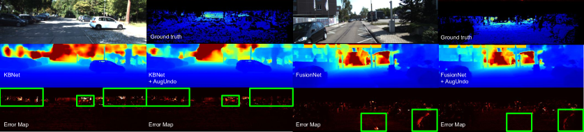
Figure 3: Qualitative comparisons on KITTI. We compare KBNet and FusionNet trained using standard augmentations and trained with AugUndo. AugUndo consistently produces lower errors in highlighted regions where structures may have arbitrary orientation (vegetation) and regions near image border that typically lacks correspondence during training. See error maps for comparisons. Best viewed in 2$\times$.

Experiment setup. Code of each work is obtained from their respective Github repository; we followed their settings and modified data handling and loss function to incorporate AugUndo. For each setting, we perform 4 independent trials for each model and report the means and standard deviations over all trials. To ensure fair comparison, we train all models from scratch. Implementation details can be found in Sec. A of the Supp. Mat. For augmentations, we experimented with a range of combinations both in the type and values chosen. Below, we report the best combination through extensive experiments on each dataset. Evaluation metrics used are detailed in Table 5 in the Supp. Mat.

5.1 Results on VOID

Augmentations. Through a search over augmentation types and values, we found a consistent set of augmentations that tends to yield improvements across all methods with small changes to degree of augmentation catered to each method. We applied photometric transformations of random brightness from 0.5 to 1.5, contrast from 0.5 to 1.5, saturation from 0.5 to 1.5, and hue from -0.1 to 0.1. We applied image patch removal by selecting between 0.1% to 0.5% of the pixels and removing 5 $\times$ 5 patches centered on them – approximately removing between 2.5% to 12.5% of the image. We applied random sparse depth point removal at a rate between 60% and 70% of all sparse points. We further applied geometric transformations of random horizontal and vertical flips, up to 10% of translation and between -25 to 25 degrees of rotation. For KBNet and FusionNet, we applied random resize factor between 0.6 to 1.4, while for VOICED, we used 0.7 to 1.3 because the scaffolding step of VOICED requires at least 3 points, but as discussed above, resampling causes loss and factors smaller than 0.7 often cause all points to be dropped. Augmentations are applied with a 50% probability. Rows in Table 1 and 2 marked with ”+ AugUndo” denote models trained with our method.

Method	MAE $\downarrow$	RMSE $\downarrow$	iMAE $\downarrow$	iRMSE $\downarrow$
VOICED	318.59$\pm$7.74	1,213.60$\pm$17.49	1.30$\pm$0.05	3.72$\pm$0.04
+ AugUndo	295.41$\pm$0.30	1,159.27$\pm$5.44	1.20$\pm$0.02	3.49$\pm$0.03
FusionNet	285.55$\pm$2.16	1,174.47$\pm$10.67	1.20$\pm$0.03	3.45$\pm$0.08
+ AugUndo	267.69$\pm$1.85	1,157.07$\pm$4.61	1.08$\pm$0.02	3.19$\pm$0.03
KBNet	263.90$\pm$3.63	1,130.66$\pm$6.22	1.05$\pm$0.01	3.24$\pm$0.04
+ AugUndo	256.37$\pm$1.00	1,114.53$\pm$3.79	1.01$\pm$0.01	3.13$\pm$0.03

Table 4: Results of on KITTI. AugUndo consistently improves all methods for all metrics by approximately 5.2% on average.

Results. Table 1 (left, VOID1500) shows our main results on the VOID depth completion benchmark. By training the models with our augmentation strategy, we observe an average overall improvement of 18.3% across all methods and metrics on VOID1500. Specifically, we improve VOICED by 26.4%, FusionNet by 16.3%, and KBNet by 12.2%. These experiments validate our hypothesis that by applying a wider range of augmentations, we are able to improve the baseline model’s performance. They also illustrate the lack in use of augmentations in existing works: incorporating standard augmentations (albeit requiring modification to augmentation and loss computation pipelines) can yield a large performance boost. Fig. 2 shows a head-to-head comparison between KBNet trained using standard procedure in [41] and KBNet trained using AugUndo. We observe qualitative improvements from AugUndo where we improve KBNet in homogeneous regions and image borders, i.e., pillar (left), cabinet (middle), wall (right). Including the geometric augmentations consistently yields fewer border artifacts as we apply random translation, which warps part of the image out of frame. This allows us to simulate occlusion due to motion (i.e. forward), where the borders of the image that do not have correspondence in another frame. In the standard training scheme, this results in failures to recover structures near the image border, but with AugUndo we can render models robust to them by computing the loss on the original frame of reference (where we do have correspondence) through our inverse transformations of the depth map. Additionally, resizing allows the model to learn multiple resolutions of the input, akin to zooming in and out, which can also impose smoothness in homogeneous regions through the scale-space transition; whereas, rotation can simulate diverse camera orientations. Fig. 2 shows that translation, rotation and resizing can model these effect in the input space, but with a loss computed without the induced nuisance and on the original image.

Sensitivity study. One limitation of existing training pipelines is that there are little to no augmentations applied to sparse depth modality. However, in real-world applications, sparse depth in fact has a high variability, i.e., features tracked in SLAM/VIO systems will vary depending on the scene (points are dropped or added to the state), and point cloud densities returned by a sensor will differ based on specifications. To further examine the effect of AugUndo on sparse depth, we study the sensitivity to changes in sparse depth density by testing models on VOID1500 ($\approx$1500 points) on VOID500 ($\approx$500). For the 3$\times$ reduction in sparse points, AugUndo improves robustness by an average of 23.1% across all methods This is thanks to the use of geometric and occlusion augmentations made possible by AugUndo, which greatly increase sparse depth variations, i.e. decimating them through resizing, re-orienting their configuration through rotation, translating them out of frame, and randomly occluding them, to avoid overfitting particular sparse depth configurations. We further push their limits in Table 6 of the Supp. Mat., where we test them on VOID150 with a 10$\times$ reduction in sparse points from the training set (VOID1500) and observe the same trend of improvements. This showcases the benefits of AugUndo for improving robustness of models to changes in sparse depth.

Zero-shot generalization. We test models trained on VOID on NYUv2 and ScanNet. Table 2 shows an average of 23.2% improvement on NYUv2 and 27.6% on ScanNet. Applying our method to VOICED greatly improve the zero-shot generalization ability on both NYUv2 and ScanNet. This is likely due to the scaffolding densification employed by VOICED, where the network can overfit to the scaffoldings of particular sparse depth configuration and therefore, does not generalize well when presented with sparse depth map with a different configuration. Like our sensitivity study (Fig. 2, VOID500), occlusion and geometric augmentations introduce variation into the sparse depth configurations and densities, which alleviates overfitting to specific point clouds or 3D scenes; hence, improving VOICED from 49.9% and 52.6% on NYUv2 and ScanNet, respectively. For FusionNet and KBNet, we see smaller improvements, but still nontrivial: FusionNet improves by 8% and 12.1% on NYUv2 and ScanNet, and KBNet by 11.7% and 18.3%. This further validates our hypothesis that by applying a more diverse set of transformations, we are able to improve generalization to new datasets.

Ablation study. Table 3 shows a comprehensive ablation study following augmentation settings above. From our best reported settings on KBNet, we removed individual augmentations to show their empirical contribution. Note: random brightness, contrast, saturation, and hue (BRI, SAT, CON, HUE) together is the standard color jitter employed by all current methods. We also test removing all color jitter augmentations to further quantify its effect.

We found that random flips (FLP) has the largest impact of all of the augmentations – increasing the error by an average of 30%; this is because it simulates different scene layouts. As there are no viable intensity augmentations for sparse depth, RMP is the only one to explicitly increase variability in the data modality hence it also has large influence. We note that other geometric augmentations contribute as well, i.e. rotation, resizing and translation, to discard points. By computing the loss on the original inputs, we reconstruct the removed points, which in fact serves as an additional training signal to map RGB to depth.

Photometric augmentations, individually, have small effect on performance. To get a non-neglible effect, one must disable all color jitter (Table 3 , row 7), which still yielded small increases in errors. This shows the limitations of existing augmentations, which relies heavily on color jittering. We note that we use a larger value range in color jitter than existing works, so the impact is expected to be even smaller for existing works. Admittedly, the most important one (FLP) is currently being used by all methods, but resize, image patch and point removal, play a large role. The best results are obtained when using all of the proposed augmentations, demonstrating the importance of scaling up both photometric and geometric augmentations.

5.2 Results on KITTI

Augmentations. We applied random brightness, random contrast, random saturation from 0.5 to 1.5 and random hue from -0.1 to 0.1. We applied image patch removal by selecting between 0.1% to 0.5% of the pixels and removing 5 $\times$ 5 patches centered on them. We applied random sparse depth point removal at a rate between 60% and 70% of all sparse points. We further applied random horizontal flips, up to 10% of translation, resizing factors between 0.8 to 1.2, and between -20 to 20 degrees of rotation. We found that vertical flips are detrimental to performance.

Results. While AugUndo consistently improves all methods (Table 4), we note that the improvement is less, but respectable, in this case: $\approx$5.2% overall with the largest gain in FusionNet of 6.41%. This is largely due to the small scene variations in the outdoor driving scenarios, i.e. ground plane with vehicles, buildings ahead and on the sides, horizontal lidar scans, and largely planar motion. The dataset bias is strong enough to render vertical flip detrimental to performance. This is also evident in existing works as none utilizes vertical flip as augmentation. Nonetheless, AugUndo still improves performance, where point removal models different lidar returns patterns, and resizing simulates large variations in scales of objects observed in road scenes. Similar to indoors, translations help model occlusuions due to large motions. We note that the performance improvements are also obtained nearly for free as AugUndo only add negligible time to training. The percentage gain, however, is similar to that of innovating a new method, i.e. architectural design, such as the improvement of FusionNet over VOICED and KBNet over FusionNet.

Fig. 3 compares FusionNet and KBNet trained using conventional augmentations and AugUndo. AugUndo improves over objects that may have diverse orientations (such as tree branches and vegetation), thanks to rotation augmentations. Improvements are also observed in the far regions where resizing can help simulate closer objects in far distances. As we use translation and occlusion augmentations, AugUndo also improves on occlusion boundaries and regions occluded by motion during training (highlighted), which makes estimates near image borders more robust.

6 Discussion

Conventionally, data augmentation aims to seek visual invariance and create a collection of equivalent classes, i.e., identifying an image and its augmented variant as the same. For geometric tasks, the underlying equivalence is in the 3D scene structures under various illumination conditions, camera, viewpoints, occlusion, etc. Assuming a rigid scene, the shapes populating it should persist regardless of the nuisance variables. This motivates the use of geometric augmentations, as it simulates the nuisances within the image, but, when used naively, disrupts the model instead. Effective use of geometric augmentations in unsupervised depth completion are obstructed by artifacts introduced during the transformations. AugUndo lifts this obstacle by “undo-ing” the augmentations before computing the loss.

While AugUndo enables scaling up augmentations for unsupervised training, i.e. depth completion, it may also be applicable for supervised methods; though, we posit that the gain to be less as the artifacts induced from photometric and geometric augmentations of an image tend to be larger than those of a piece-wise smooth depth map. Our method is also limited to 2D augmentations; whereas, the nuisances modeled by our method are projections of the 3D scene. We leave extensions to 3D for future work. We also only consider a single image and sparse depth map as input. Likewise, extensions can be made towards multi-frame geometric tasks such as stereo, optical flow, etc., but one must account for their specifics and problem setups, i.e. stereo assumes frontoparallel views. This is outside of our scope, so we leave them as future directions. This work paves way for the empirical success in unsupervised geometric tasks that we have observed in other visual recognition tasks.

Supplementary Material

Appendix A Implementation details

We implemented our method in PyTorch and incorporated our augmentation pipeline into the codebases of VOICED [42], FusionNet [43], and KBNet [41]. The models are optimized using Adam [19] with $\beta_{1}=0.9$ and $\beta_{2}=0.999$. For VOID: We used an input batch size of 12, and a random crop size of $416\times 512$ for KBNet and a batch size of 8 without cropping for FusionNet and VOICED. We trained each KBNet model for 40 epochs with base learning rate of $1\times 10^{-4}$ for 20 epochs and decreased to $5\times 10^{-5}$ for the last 20 epochs. We trained FusionNet and VOICED for 20 epochs with a base learning rate of $1\times 10^{-4}$ for 10 epochs and decreased to $5\times 10^{-5}$ for the last 10 epochs. For KITTI: We used a batch size of 8 and random crop size of 320 by 768 for all models. We trained KBNet for 60 epochs, with $5\times 10^{-5}$ for 2 epochs, $1\times 10^{-4}$ until 8th epoch, $2\times 10^{-4}$ until 30th epoch, $1\times 10^{-4}$ until the 45th epoch and $5\times 10^{-5}$ until the 60th epoch. We trained FusionNet for 30 epochs $2\times 10^{-4}$ for 16 epochs, $1\times 10^{-4}$ until 24th epoch and $5\times 10^{-5}$ until the 30th epoch. We trained VOICED for 30 epochs $2\times 10^{-4}$ for 16 epochs, $6\times 10^{-5}$ until 24th epoch and $3\times 10^{-5}$ until the 30th epoch.

We ensure that all baseline methods can reproduce or exceed the numbers originally reported by the authors. All reported results of AugUndo are based on those same settings with the exception of the augmentation scheme.

Appendix B Evaluation metrics

The evaluation metrics that we use are shown in Table 5.

Metric	Definition
MAE	$\frac{1}{|\Omega|}\sum_{x\in\Omega}|\hat{d}(x)-d_{gt}(x)|$
RMSE	$\big{(}\frac{1}{|\Omega|}\sum_{x\in\Omega}|\hat{d}(x)-d_{gt}(x)|^{2}\big{)}^{1/2}$
iMAE	$\frac{1}{|\Omega|}\sum_{x\in\Omega}|1/\hat{d}(x)-1/d_{gt}(x)|$
iRMSE	$\big{(}\frac{1}{|\Omega|}\sum_{x\in\Omega}|1/\hat{d}(x)-1/d_{gt}(x)|^{2}\big{)}^{1/2}$

Table 5: Error metrics. $d_{gt}$ denotes the ground-truth depth.

0:   Depth completion network $f_{\theta}$, Images $I_{t},I_{\tau}$, Sparse depth $z_{t}$, Relative pose $g_{rt}$, Intrinsics $K$

1:   Sample $\{T_{pt,I}^{1}\ldots T_{pt,I}^{k}\}$ from $T_{pt,I}^{i}\in\mathcal{A}_{pt,I}$, and compose $T_{pt,I}=T_{pt,I}^{1}\circ T_{pt,I}^{2}\circ\cdots\circ T_{pt,I}^{k}$

2:   Sample $\{T_{pt,z}^{1}\ldots T_{pt,z}^{j}\}$ from $T_{pt,z}^{i}\in\mathcal{A}_{pt,z}$, and compose $T_{pt,z}=T_{pt,z}^{1}\circ T_{pt,z}^{2}\circ\cdots\circ T_{pt,z}^{j}$

3:   Sample $\{T_{ge}^{1}\ldots T_{ge}^{m}\}$ from $T_{ge}^{i}\in\mathcal{A}_{ge}$, and compose $T_{ge}=T_{ge}^{1}\circ T_{ge}^{2}\circ\cdots\circ T_{ge}^{m}$

4:   Compose the inverse geometric transform $T_{ge}^{-1}=({T_{ge}^{m}})^{-1}\circ(T_{ge}^{m-1})^{-1}\circ\cdots\circ({T_{ge}^{1}})^{-1}$

5:   Compute the coordinates after geometric transform $\begin{bmatrix}x^{\prime}&1\end{bmatrix}^{\top}=T_{ge}\begin{bmatrix}x&1\end{bmatrix}^{\top}$ (Eqn. 3 from main paper)

6:   Augment $I_{t}$ with photometric and geometric transformations $I_{t}^{\prime}(x^{\prime})=T_{pt,I}(I_{t})(x)$ (Eqn. 4 from main paper)

7:   Augment $z_{t}$ with occlusion and geometric transformations $z_{t}^{\prime}(x^{\prime})=T_{pt,z}(z_{t})(x)$ (Eqn. 4 from main paper)

8:   Obtain depth prediction $\hat{d}^{\prime}_{t}=f_{\theta}(I^{\prime}_{t},z^{\prime}_{t})$

9:   Compute coordinates of the inverse geometric transformation $\begin{bmatrix}x^{\prime\prime}&1\end{bmatrix}^{\top}=T^{-1}_{ge}\begin{bmatrix}x^{\prime}&1\end{bmatrix}^{\top}$ (Eqn. 5 from main paper)

10:   Apply inverse geometric transformation on output depth map: $\hat{d}_{t}(x^{\prime\prime})=\hat{d}_{t}^{\prime}(x^{\prime})$ (Eqn. 6 from main paper)

11:   Reconstruct $I_{t}$ from $I_{\tau}$ using Eqn. 1 from main paper, i.e., $\hat{I}_{t\tau}=I_{\tau}(\pi g_{\tau t}K^{-1}\bar{x}\hat{d}_{t})$

12:   Minimize reconstruction losses between $\hat{I}_{t\tau}$ and $I_{t}$, and $\hat{d}_{t}$ and $z_{t}$, and the regularizer (Eqn. 2 from main paper)

Algorithm 1 AugUndo for Unsupervised Depth Completion

Method	MAE $\downarrow$	RMSE $\downarrow$	iMAE $\downarrow$	iRMSE $\downarrow$	MAE $\downarrow$	RMSE $\downarrow$	iMAE $\downarrow$	iRMSE $\downarrow$
Dataset	VOID500				VOID150
VOICED	137.01$\pm$4.23	235.80$\pm$7.82	71.36$\pm$1.86	130.63$\pm$5.66	209.59$\pm$5.18	329.71$\pm$10.01	130.45$\pm$5.63	229.79$\pm$14.09
+ AugUndo	92.99$\pm$1.11	176.94$\pm$1.38	46.43$\pm$0.85	91.10$\pm$1.64	151.77$\pm$1.99	262.61$\pm$2.19	88.65$\pm$0.76	169.29$\pm$2.71
FusionNet	97.73$\pm$0.73	194.32$\pm$1.36	58.65$\pm$1.31	122.95$\pm$3.04	158.03$\pm$1.97	284.23$\pm$3.05	113.67$\pm$2.03	223.41$\pm$0.93
+ AugUndo	74.97$\pm$1.15	162.71$\pm$1.86	40.44$\pm$1.09	92.11$\pm$1.01	126.16$\pm$1.44	246.16$\pm$2.46	86.13$\pm$4.46	181.08$\pm$8.00
KBNet	78.44$\pm$1.39	178.17$\pm$3.27	37.56$\pm$0.61	83.43$\pm$1.89	149.13$\pm$3.29	306.30$\pm$8.74	70.74$\pm$2.26	136.75$\pm$5.55
+ AugUndo	66.97$\pm$0.81	151.55$\pm$2.03	31.63$\pm$0.53	71.90$\pm$0.82	117.16$\pm$4.51	239.60$\pm$10.96	57.65$\pm$1.47	112.81$\pm$1.75

Table 6: Sensitivity study of depth completion on VOID. Reported scores are mean and standard deviation over four independent trials. We compare the sensitivity of models trained on VOID1500, with standard augmentations and AugUndo, by testing them on VOID500 and VOID150. Sparse depth maps within VOID1500 contains approximately 1500 points, and those within VOID500 and VOID150 contain approximately 3$\times$ and 10$\times$ less, respectively. AugUndo improves performance by an average of 23.09% and 21.85% across all methods and evaluation metrics on VOID500 and VOID150, respectively.

Appendix C Datasets

KITTI [10] contains 61 driving scenes with research in autonomous driving and computer vision. It contains calibrated RGB images with sychronized point clouds from Velodyne lidar, inertial, GPS information, etc. For depth completion [39], there are $\approx$80,000 raw image frames and associated sparse depth maps, each with a density of $\approx$5%. Ground-truth depth is obtained by accumulating 11 neighbouring raw lidar scans. Semi-dense depth is available for the lower $30\%$ of the image space. We test on the official validation set of 1,000 samples because the online test server has submission restrictions to accomodate multiple trials. For depth estimation, we used Eigen split [4], following [51] to preprocess and remove static frames. The remaining training set contains 39,810 monocular triplets and the validation set contains 4,424 triplets. The testing set contains 697 monocular images. We follow the evaluation protocol of [39, 5], where output depth is evaluated where ground truth exists between 0 to 80.0 meters.

VOID [42] comprises indoor (laboratories, classrooms) and outdoor (gardens) scenes with synchronized $640\times 480$ RGB images and sparse depth maps. XIVO [7], a VIO system, is used to obtain the sparse depth maps that contain approximately 1500 sparse depth points with a density of about 0.5%. Active stereo is used to acquire the dense ground-truth depth maps. In contrast to the typically planar motion in KITTI, VOID has 56 sequences with challenging 6 DoF motion captured on rolling shutter. 48 sequences (about 45,000 frames) are assigned for training and 8 for testing (800 frames). We follow the evaluation protocol of [42] where output depth is evaluated where ground truth exists between 0.2 and 5.0 meters.

NYUv2 [36] consists of 372K synchronized $640\times 480$ RGB images and depth maps for 464 indoors scenes (household, offices, commercial), captured with a Microsoft Kinect. The official split consisting in 249 training and 215 test scenes. We use the official test set of 654 images. Because there are no sparse depth maps provided, we sampled $\approx 1500$ points from the depth map via Harris corner detector [14] to mimic the sparse depth produced by SLAM/VIO. We test models trained on VOID to evaluate their generalization to NYUv2. We follow the evaluation protocol of [42] where output depth is evaluated where ground truth exists between 0.2 and 5.0 meters.

ScanNet [3] consists of RGB-D data for 1,513 indoor scenes with 2.5 million images and corresponding dense depth map. Because there are no sparse depth maps provided, we sampled $\approx 1500$ points from the depth map via Harris corner detector [14] to mimic the sparse depth produced by SLAM/VIO. We followed [3] and used 100 scenes (scene707-scene806), for zero-shot generalization for models trained on VOID. The output depth is evaluated where ground truth exists between 0.2 and 5.0 meters.

Waymo Open Dataset [37] contains 1920$\times$1280 RGB images and lidar scans from autonomous vehicles. The training set contains $\approx$158K images from 798 scenes and the validation set $\approx$40K images from 202 scenes, collected at 10Hz. Objects are annotated across the full 360^∘ field. Sparse depth maps are obtained by reprojecting the point cloud scan from the top lidar to the camera frame. Ground truth is obtained by reprojecting both front facing lidars as well as those collected 10 time steps forward and backwards (approximately 1 second of capture) to a given camera frame at a specific time step to densify the sparse depth. We used the object annotations to remove all moving objects to ensure that reprojected points respects the static scene assumption. We also performed outlier removal to filter out errorenous (noisy) points. The output depth is evaluated where ground truth exists between a 1.5 and 80.0 meters range.

Appendix D The AugUndo Algorithm

We assume that we are given (i) $I:\Omega\subset\mathbb{R}^{2}\rightarrow\mathbb{R}^{3}_{+}$ an RGB image $I_{t}$, (ii), its associated sparse point cloud projected onto as a depth map $z:\Omega_{z}\subset\Omega\rightarrow\mathbb{R}_{+}$, $z_{t}$, (iii) camera intrinsic calibration matrix $K\in\mathbb{R}^{3\times 3}$, (iv) a sequence of images $I_{\tau}$ for $\tau\in\{t-1,t+1\}$ during training, and (v) the relative pose $g_{\tau t}$ between the image frame $I_{t}$ and some temporally adjacent image $I_{\tau}$. Given a image and its associated sparse depth map, a depth completion network learns a map the inputs to the output depth map $\hat{d}_{t}:=f_{\theta}(I_{t},z_{t})\in\mathbb{R}_{+}^{H\times W}$. In the main paper, we denoted photometric and occlusion augmentations as $\mathcal{A}_{pt}$ for ease of notation. Here, for specificity, we define $\mathcal{A}_{pt,I}$ as the set of possible photometric (including occlusion) transformations for the image, $\mathcal{A}_{pt,z}$ as the possible set of occlusion augmentations for sparse depth maps, and $\mathcal{A}_{ge}$ as the possible set of all geometric transformations. We additionally assumes we have the set of geometric transformations $T_{ge}$ used during augmentation and their inverse transformations $T^{-1}_{ge}$. Alg. 1 is the procedural algorithm of AugUndo and details the step by step augmentation and loss computation pipelines, given our inputs.

Dataset	Method	MAE $\downarrow$	RMSE $\downarrow$	iMAE $\downarrow$	iRMSE $\downarrow$
Waymo	VOICED	6781.27$\pm$317.21	7734.57$\pm$339.77	24.58$\pm$1.45	27.87$\pm$1.63
	+ AugUndo	5965.07$\pm$367.47	7029.66$\pm$509.43	18.54$\pm$1.83	22.10$\pm$3.96
	FusionNet	530.55$\pm$39.23	1734.23$\pm$114.97	1.27$\pm$0.12	2.82$\pm$0.29
	+ AugUndo	512.29$\pm$8.43	1707.34$\pm$48.25	1.21$\pm$0.09	2.75$\pm$0.18
	KBNet	625.00$\pm$12.47	2167.74$\pm$92.17	1.76$\pm$ 0.13	5.46$\pm$0.93
	+ AugUndo	541.29$\pm$15.16	2014.14$\pm$76.52	1.34$\pm$0.11	3.43$\pm$0.30

Table 7: Quantitative results of zero-shot transfer from KITTI to Waymo. AugUndo improves generalization of models trained on KITTI to Waymo by an average of 13.3% for all evaluation metrics. We note that the sparse depth maps provided in Waymo is considerably denser than KITTI as they are merged from two front separate lidars; hence, FusionNet, which employs a learned (frozen) densification network performs similarly, i.e., the bias introduced by the same frozen densification network (ScaffNet) is strong enough that FusionNet yields similar results for both conventional augmentation scheme and AugUndo. Nonetheless, we still observe considerable improvements.

Method	MAE $\downarrow$	RMSE $\downarrow$	iMAE $\downarrow$	iRMSE $\downarrow$
MonDi	37.31$\pm$0.88	87.34$\pm$3.16	20.05$\pm$1.76	44.15$\pm$1.31
+ AugUndo	34.33$\pm$0.98	83.22$\pm$1.55	16.94$\pm$0.70	41.40$\pm$1.08

Table 8: Quantitative results of an unsupervised distillation-based method on VOID1500. Reported scores are mean and standard deviation over four independent trials. Training with AugUndo improves MonDi performance by an average of 8.6% across evaluation metrics on VOID1500.

Appendix E Sensitivity Study for Depth Completion

Given that conventional augmentation pipelines are not applied towards sparse depth modality, it is possible that a model will overfit to the sparse point cloud, which describes the coarse 3D scene structure. Overfitting to scenes, hence, can limit generalization and increase sensitivity to the configuration of sparse points. Hence, we test the effect of AugUndo on various sparse depth input densities. We presented results on VOID500 and VOID150 in Table 6 (left and right, respectively). VOID500 contains approximately 500 sparse points per point cloud and VOID150 contains approximately 150 points. All models tested are trained on VOID1500, which contains 1500 sparse points.

For VOID500 (Table 6, left), which is a 3$\times$ reduction in density, AugUndo improves the sensitivity to changes in the sparse points by an average of 23.09% across all methods, and 30.57%, 23.92%, and 14.79% for VOICED, FusionNet, and KBNet, respectively. For an even more challenging scenario, also the closest setup to the density of sparse points tracked by a Simultaneous Localization and Mapping (SLAM) and Visual Inertial Odometry (VIO) system, we consider VOID150 (Table 6, right). Here, AugUndo improves by an angerage of 21.85% across all methods, and 26.57%, 19.18%, and 19.80% for VOICED, FusionNet, and KBNet, respectively. We attribute this to geometric and occlusion augmentations: translation, resize, rotation and sparse points removal. All of these augmentations not only affect photometry, but also the sparse point cloud where points are dropped due to resampling or explicitly removed, and additionally point cloud orientation is also altered.

Appendix F Zero-shot Generalization from KITTI

In the main paper, we demonstrated AugUndo for three unsupervised methods [42, 43, 41] on the KITTI dataset. Due to space constraints, here, we provide additional results for zero-shot generalization from KITTI to Waymo Open Dataset [37] in Table 7. Overall, training with AugUndo improves existing methods by an average 13.3% across all evaluation metrics.

We note that AugUndo improves VOICED and KBNet by larger amounts than FusionNet. For FusionNet, whether trained with conventional augmentation scheme or AugUndo, both seem to perform similarly. This is because FusionNet employs a learning-based densification network (ScaffNet), which is pretrained on synthetic datasets and frozen, that is used in both models. As the sparse depth maps in Waymo are much denser than KITTI, ScaffNet is able to approximate the dense depth map with small amounts of errors. This serves as an inductive bias for the downstream FusionNet, which learns the residual over the approximated depth map. As the reconstruction from ScaffNet exhibits high fidelity, the bias induced by ScaffNet on FusionNet causes FusionNet to perform only minor modifications to approximated depth map, leading to similar outputs whether trained with conventional augmentations or AugUndo. Nonetheless, we still observe consistent (albeit smaller) improvements when FusionNet is trained with AugUndo.

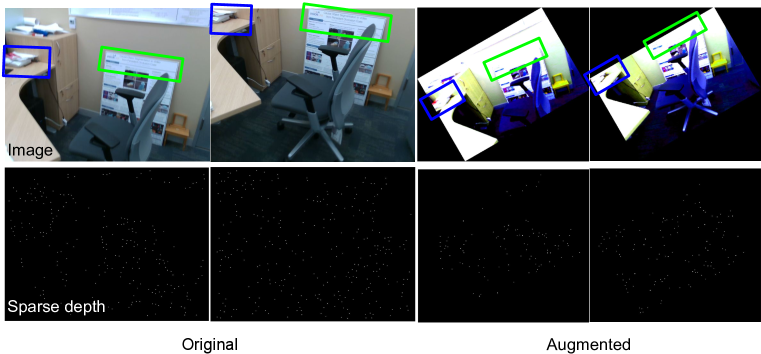
Figure 4: Motivation. After augmenting the inputs with photometric and geometric transformations, the previously exciting image textures (for establishing correspondence across images) and sparse points in the original inputs, that would have served as supervision, are now largely saturated in intensity and homogenous, and lost due to resampling, respectively (best viewed in 2$\times$).

Appendix G Additional Quantitative Results on VOID

In the main paper, we demonstrated AugUndo for three unsupervised methods [42, 43, 41] on the VOID dataset. Due to space constraints, here, we show additional results on VOID1500 for a recent unsupervised distillation method, MonDi [24], in Table 8. We applied photometric transformations of random brightness from 0.5 to 1.5, contrast from 0.5 to 1.5, saturation from 0.5 to 1.5, and hue from -0.1 to 0.1. We applied image patch removal by selecting between 0.1% to 0.5% of the pixels and removing 5 $\times$ 5 patches centered on them – approximately removing between 2.5% to 12.5% of the image. We applied random sparse depth point removal at a rate between 60% and 95% of all sparse points. We further applied geometric transformations of random horizontal and vertical flips, up to 10% of translation, between -25 to 25 degrees of rotation, and random resize factor between 0.6 to 1.4.

Overall, we improve MonDi by an average of 8.6% across all evaluation metrics. This is surprising as amongst all the tested methods, MonDi is the most light-weight, with only 5.3M parameters. As we reduce model capacity, one would expect that the network to saturate in the data variations that can be modeled. However, despite the size of network is much smaller (23.2% less than KBNet), there is still a considerable gain when using AugUndo instead of their augmentation pipeline. This demonstrates efficacy and applicability of AugUndo; it can be used to improve methods with a range of capacities from tens of millions to several million. Also, we note that MonDi is an unsupervised distillation method (where it distills from unsupervised methods), so it is more closely related to supervised methods in supervision than unsupervised method. Even so, we observe a non-trivial improvement, which validates our discussion in Sec. 6 of the main paper regarding the applicability of AugUndo to supervised methods.

Appendix H Extended Discussion of Motivation

In the main paper, we discussed the motivation behind the approach. Here, we provide an extended discussion: Training unsupervised depth completion methods relies on a photometric reconstruction term, sparse depth reconstruction term, and a (generic) regularizer, such as local smoothness. The photometric reconstruction term constraints the solution in regions where there are sufficiently exciting textures and co-visible between images such as those highlighted in Fig. 4. The sparse depth reconstruction term constraints the solution anywhere with a sparse point. Everywhere else in the image are inherently ambiguous, so we must rely on the regularizer. Fig. 4 shows that after one has applied a number of photometric and geometric transformations, the previously exciting textures that would have served as our supervision are now largely saturated in intensity and homogenous. The number of points in the sparse depth maps have also been greatly reduced.

In conventional augmentation scheme for other (semantic) vision tasks, i.e. classification, detection, and segmentation, it is typical for one to introduce saturation in image intensities, block artifacts from interpolation and loss during resampling. These are some of the side-effects that are desirable in the aforementioned tasks: introducing these nuisance variabilities enables the model to learn to be invariant to them (i.e., to learn them away), which yields more generalizable and robust representations. However, this is not the case for learning unsupervised depth. Because the supervision signal comes from reconstructing the input image and sparse depth map, the more we augment the data (causing a loss of photometric correspondences across image frames and a loss of points in the sparse depth map), the more we degrade the supervision signal. So it is not too surprising that conventional augmentation procedures, both photometric and geometric, have seen limited use beyond small changes in image intensities, and flipping.

Nevertheless, photometric augmentations help model the diverse range of illumination conditions and colors of object that may populate the scene. Geometric augmentations can simulate the various camera motion, for example, image translations can approximate small baseline movements, and in-plane rotations can model camera orientation. These augmentations are often viewed as essential to training pipelines for other vision tasks, but are detrimental for unsupervised depth completion; yet, without them, one may encounter robustness and generalization issues. As the root of the problem lies in the supervision signal, we investigate an approach to “undo” the augmentations during (or right before) the loss computation step. Doing so enables one to feed forward augmented inputs, but compute the loss on the original inputs with no loss in the training signal. Extensive experiments show that our approach improves performance and zero-shot generalization across a number of methods for both indoor and outdoor scenarios.

Method	MAE $\downarrow$	RMSE $\downarrow$	Abs Rel $\downarrow$	Sq Rel $\downarrow$	$\delta<1.25\uparrow$	$\delta<1.25^{2}\uparrow$	$\delta<1.25^{3}\uparrow$
Monodepth2	283.861$\pm$3.732	395.947$\pm$5.728	0.183$\pm$0.002	0.100$\pm$0.003	0.717$\pm$0.005	0.922$\pm$0.004	0.975$\pm$0.002
+ AugUndo	277.696$\pm$4.861	388.088$\pm$5.768	0.178$\pm$0.003	0.095$\pm$0.004	0.724$\pm$0.007	0.925$\pm$0.004	0.978$\pm$0.002
HR-Depth	286.282$\pm$7.059	399.112$\pm$9.184	0.185$\pm$0.004	0.100$\pm$0.004	0.714$\pm$0.012	0.919$\pm$0.006	0.975$\pm$0.002
+ AugUndo	283.086$\pm$6.787	394.261$\pm$9.133	0.181$\pm$0.005	0.097$\pm$0.005	0.718$\pm$0.013	0.922$\pm$0.004	0.977$\pm$0.002
Lite-Mono	319.910$\pm$15.00	446.005$\pm$22.97	0.209$\pm$0.013	0.129$\pm$0.019	0.669$\pm$0.016	0.892$\pm$0.011	0.963$\pm$0.006
+ AugUndo	308.010$\pm$0.859	426.626$\pm$0.484	0.200$\pm$0.003	0.114$\pm$0.001	0.674$\pm$0.005	0.901$\pm$0.002	0.969$\pm$0.002

Table 9: Quantitative results of monocular depth estimation on VOID. AugUndo also consistently improves three monocular depth models.

Dataset	Method	MAE $\downarrow$	RMSE $\downarrow$	Abs Rel $\downarrow$	Sq Rel $\downarrow$	$\delta<1.25\uparrow$	$\delta<1.25^{2}\uparrow$	$\delta<1.25^{3}\uparrow$
NYUv2	Monodepth2	0.432$\pm$0.003	0.556$\pm$0.005	0.205$\pm$0.001	0.159$\pm$0.001	0.683$\pm$0.005	0.907$\pm$0.001	0.975$\pm$0.001
	+ AugUndo	0.415$\pm$0.005	0.537$\pm$0.006	0.196$\pm$0.002	0.148$\pm$0.003	0.700$\pm$0.008	0.915$\pm$0.002	0.977$\pm$0.001
	HR-Depth	0.424$\pm$0.003	0.549$\pm$0.003	0.201$\pm$0.002	0.154$\pm$0.002	0.692$\pm$0.003	0.910$\pm$0.002	0.976$\pm$0.001
	+ AugUndo	0.421$\pm$0.009	0.542$\pm$0.011	0.199$\pm$0.005	0.152$\pm$0.006	0.696$\pm$0.009	0.913$\pm$0.004	0.976$\pm$0.001
	Lite-Mono	0.480$\pm$0.012	0.616$\pm$0.018	0.231$\pm$0.008	0.199$\pm$0.015	0.637$\pm$0.009	0.879$\pm$0.009	0.964$\pm$0.004
	+ AugUndo	0.468$\pm$0.003	0.595$\pm$0.003	0.225$\pm$0.004	0.187$\pm$0.005	0.646$\pm$0.002	0.889$\pm$0.003	0.968$\pm$0.001
ScanNet	Monodepth2	0.284$\pm$0.004	0.368$\pm$0.005	0.177$\pm$0.002	0.097$\pm$0.002	0.741$\pm$0.006	0.931$\pm$0.003	0.980$\pm$0.001
	+ AugUndo	0.270$\pm$0.003	0.351$\pm$0.004	0.169$\pm$0.001	0.088$\pm$0.002	0.759$\pm$0.004	0.937$\pm$0.001	0.982$\pm$0.001
	HR-Depth	0.282$\pm$0.004	0.366$\pm$0.005	0.175$\pm$0.002	0.095$\pm$0.002	0.743$\pm$0.005	0.929$\pm$0.003	0.979$\pm$0.002
	+ AugUndo	0.274$\pm$0.007	0.357$\pm$0.009	0.172$\pm$0.005	0.092$\pm$0.005	0.754$\pm$0.009	0.935$\pm$0.003	0.981$\pm$0.001
	Lite-Mono	0.296$\pm$0.002	0.388$\pm$0.007	0.185$\pm$0.003	0.109$\pm$0.006	0.731$\pm$0.002	0.921$\pm$0.002	0.976$\pm$0.001
	+ AugUndo	0.296$\pm$0.001	0.382$\pm$0.001	0.185$\pm$0.001	0.105$\pm$0.002	0.728$\pm$0.002	0.924$\pm$0.001	0.977$\pm$0.001

Table 10: Zero-shot generalization results from VOID to NYUv2 and ScanNet. AugUndo consistently improves zero-shot generalization to novel datasets.

Appendix I Application Towards Monocular Depth

In this study, we have discussed AugUndo as an augmentation pipeline for unsupervised depth completion, where one of the main challenges that AugUndo addresses is to retain the input sparse depth as supervision – without it, a single image does not afford the inference of scale. As depth completion involves both image and sparse depth modalities, removing sparse depth naturally reduces the problem to monocular depth estimation, where one infers the depth from a single image.

In this section, we show that AugUndo can be applied generically to unsupervised (or self-supervised) monocular depth estimation as well. We demonstrate AugUndo using three existing methods: Monodepth2 [12], HR-Depth [26], and Lite-Mono [48]. Similar to our experiments on unsupervised depth completion, we train the methods on indoor (VOID) and outdoor (KITTI) datasets using the conventional augmentation schemes employed by the methods and compare the resulting models with those trained using AugUndo. We additionally provide zero-shot generalization results for models trained on VOID to NYUv2 and ScanNet, and models trained on KITTI to Make3D. We note that as monocular depth is inferred, at most, up to an unknown scale, we perform scale matching during evaluation by using median scaling with respect to the ground truth.

Table 11 lists the error and accuracy metrics used for evaluating monocular depth estimation performance.

Make3D [33] contains 134 test images with $2272\times 1707$ resolution. Ground-truth depth maps are given at $305\times 55$ resolution and must be rescaled and interpolated. We use the central cropping proposed by [11] to get a $852\times 1707$ center crop of the image. We use standard Make3d evaluation protocol and metrics. We use Make3D to test the generalization of monocular depth estimation models trained on KITTI.

Metric	Definition
MAE	$\frac{1}{|\Omega|}\sum_{x\in\Omega}|\hat{d}(x)-d_{gt}(x)|$
RMSE	$\big{(}\frac{1}{|\Omega|}\sum_{x\in\Omega}|\hat{d}(x)-d_{gt}(x)|^{2}\big{)}^{1/2}$
AbsRel	$\frac{1}{|\Omega|}\sum_{x\in\Omega}\frac{|\hat{d}(x)-d_{gt}(x)|}{d_{gt}(x)}$
SqRel	$\frac{1}{|\Omega|}\sum_{x\in\Omega}\frac{|\hat{d}(x)-d_{gt}(x)|^{2}}{d_{gt}(x)}$
Accuracy	% of $z(x)$ s.t. $\delta\doteq\max(\frac{z(x)}{z_{gt}(x)},\frac{z_{gt}(x)}{z(x)})<$ threshold

Table 11: Error metrics. $d_{gt}$ denotes the ground-truth depth.

Method	MAE $\downarrow$	RMSE $\downarrow$	Abs Rel $\downarrow$	Sq Rel $\downarrow$	$\delta<1.25\uparrow$	$\delta<1.25^{2}\uparrow$	$\delta<1.25^{3}\uparrow$
Monodepth2	2.315 $\pm$0.005	4.794$\pm$ 0.035	0.117$\pm$ 0.001	0.845$\pm$0.030	0.869$\pm$0.004	0.959$\pm$0.001	0.982$\pm$0.001
+ AugUndo	2.237$\pm$0.014	4.739$\pm$0.032	0.113$\pm$0.000	0.862$\pm$0.030	0.879$\pm$0.002	0.960$\pm$0.001	0.982$\pm$0.001
HR-Depth	2.226 $\pm$0.004	4.626$\pm$ 0.032	0.113$\pm$0.001	0.797$\pm$0.022	0.879$\pm$0.002	0.961$\pm$ 0.001	0.982$\pm$0.000
+AugUndo	2.185$\pm$0.013	4.610$\pm$0.029	0.111$\pm$0.001	0.794 $\pm$0.021	0.883$\pm$0.001	0.962$\pm$0.001	0.983$\pm$0.001
Lite-Mono	2.338$\pm$0.005	4.821$\pm$0.027	0.121$\pm$0.001	0.875$\pm$0.007	0.862$\pm$0.002	0.955$\pm$0.001	0.980$\pm$0.000
+ AugUndo	2.314$\pm$0.030	4.780$\pm$0.055	0.120$\pm$0.001	0.849$\pm$0.019	0.863$\pm$0.004	0.955$\pm$0.001	0.981$\pm$0.001

Table 12: Quantitative results of monocular depth estimation on KITTI. AugUndo improves upon most of the metrics across different models consistently.

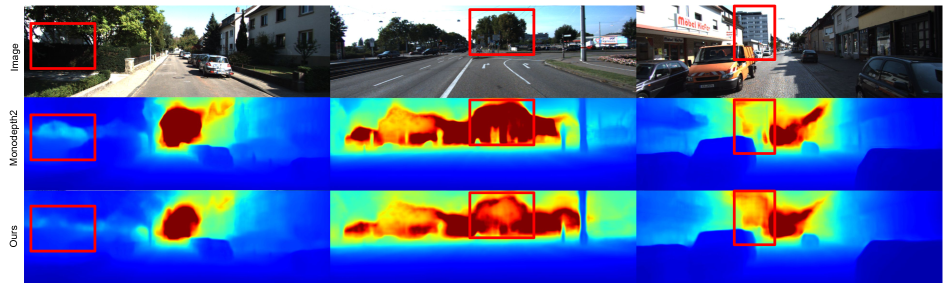
Figure 5: Qualitative result of MonoDepth2 on KITTI. Red bounding boxes highlight areas where training with our augmentation scheme improves Monodepth2, i.e., wall and vegetation on left, trees in middle and building on right.

Dataset	Method	MAE $\downarrow$	RMSE $\downarrow$	Abs Rel $\downarrow$	Sq Rel $\downarrow$	$\delta<1.25\uparrow$	$\delta<1.25^{2}\uparrow$	$\delta<1.25^{3}\uparrow$
Make3D	Monodepth2	-	7.417	0.322	3.589	-	-	-
	+ AugUndo	4.109	6.803	0.272	2.769	0.606	0.848	0.936
	HR-Depth	4.136	6.505	0.281	2.484	0.562	0.839	0.938
	+ AugUndo	4.023	6.428	0.272	2.393	0.584	0.848	0.94
	Lite-Mono	5.116	8.061	0.358	4.676	0.511	0.793	0.91
	+ AugUndo	4.728	7.518	0.321	3.887	0.529	0.817	0.926

Table 13: Generalization results on Made3D. All models are trained on KITTI. Note: for Monodepth2, we use the numbers reported by [12] and the best trial on KITTI.

Implementation details. We implement our method in PyTorch according to [12]. Specifically, we implemented our augmentation pipeline into the codebases of Monodepth2 [12], HR-Depth [26], and Lite-Mono [48]. The models are optimized using Adam [19] with $\beta_{1}=0.9$ and $\beta_{2}=0.999$. We used a input batch size of 12 and the input resolution for KITTI dataset is $640\times 192$ while the resolution for VOID is $448\times 256$. We trained the models for 20 epochs with an initial learning rate of $1\times 10^{-4}$ and drop the learning rate to $1\times 10^{-5}$ at the 15th epoch. The smoothness loss weight for KITTI is set to 0.001 as per [12] and 0.01 for VOID as VOID contains more indoor scenes with homogeneous surfaces.

We ensure that all baseline methods can reproduce or exceed the numbers originally reported by the authors. All reported results of AugUndo are based on those same settings with the exception of the augmentation scheme. Note: For Monodepth2 and HR-Depth, we initialize the ResNet encoder weight with the Imagenet-pretrained weight downloaded from PyTorch website, as specified in their Github repository. However, we cannot locate the pretrained weight used for Lite-Mono throughout their repository, which left us no choice but to train their model from scratch. Nonetheless, this does not affect the validity of the study as the comparison is made between models initialized from scratch where the difference is only in the augmentations schemes: standard convention used in the original papers and repositories, and AugUndo.

Augmentations. We applied photometric transformations of random brightness from 0.5 to 1.5, contrast from 0.5 to 1.5, saturation from 0.5 to 1.5, hue from -0.1 to 0.1. We applied geometric transformation of random rotation between -10 to 10 degrees and random horizontal flipping. We further applied random resize factor between 0.8 to 1. Augmentations are applied with a 50% probability.

Results on VOID. We present results on VOID in Table 9, where we compare the methods (Monodepth2, HR-Depth, and Lite-Mono) trained using the standard augmentations that were used in their respective papers, and AugUndo. Table 9 shows that AugUndo consistently improves all models across all error and accuracy metrics. Thus, validating the hypothesis that AugUndo can be applied generically to improve monocular depth estimation. Specifically, we observe a boost in the most difficult accuracy metric ($\delta<1.25$), where Monodepth2 improves from 0.717 to 0.724, HR-Depth from 0.714 to 0.718 and Lite-Mono from 0.669 to 0.674. At the same time, for Abs Rel metric, Monodepth2 improves from 0.183 to 0.178, HR-depth improves from 0.185 to 0.181, and Lite-Mono improves from 0.209 to 0.200.

Zero-shot generalization. To test for improvements on generalizability, we evaluate each model (Monodepth2, HR-Depth, Lite-Mono) trained on VOID by testing them for zero-shot generalizability on NYUv2 and ScanNet. The results are shown in Table 10, where training with AugUndo consistently improves generalization errors across all evaluation metrics for both NYUv2 and ScanNet. Notably, for RMSE metric, Monodepth2 improves from 0.556 to 0.537, HR-Depth from 0.549 to 0.542, Lite-Mono from 0.616 to 0.595. For ScanNet, similar improvement on RMSE can also be observed, where Monodepth2 imporves from 0.368 to 0.351, HR-Depth from 0.366 to 0.357, and Lite-Mono from 0.388 to 0.382. The improvement in RMSE metric, which is sensitive to outlier predictions, demonstrates our method’s ability to help adapt the model to a different input data distribution by exposing the models to a greater variability of nuisance variables. These trends are also observed in the case of depth completion.

Results on KITTI. We present results on KITTI in Table 12, where we compare the standard augmentation pipelines used by [12, 26, 48] and AugUndo. We observe similar trends in performance gain as we did in depth completion trained on KITTI: Applying our set of augmentations improves most metrics for all methods. We note that we observe notable improvements in $\delta<1.25$, the most difficult accuracy metric, from 0.869 to 0.879 in Monodepth2, from 0.879 to 0.883 in HR-Depth, and 0.862 to 0.863 in Lite-Mono. For Monodepth2, we also observe a large improvement in Abs Rel error, where we decreased it from 0.117 to 0.113. Similarly, for Lite-Mono, we also boosted performance across all metrics, with a particularly high improvement in Sq Rel from 0.875 to 0.849.

We note that the performance gains obtained nearly for free as our approach only affects training. We also note that the gain is similar to the improvements obtained by each successive state-of-the-art. For example, we see the improvement of Lite-Mono [48] over HR-Depth [26], and that of HR-Depth over PackNet [13] is similar to the amount of gain from AugUndo.

Applying our methods yields qualitative improvements in the depth prediction. In Fig. 5, we can see that our method produces a smoother prediction (building on the right sample) and captures ambiguous regions (vegetation on the left sample) than the baseline method, despite using the same hyper-parameter during training with the exception of data augmentation.

Zero-shot generalization. Similar to our indoor experiments, we evaluate the zero-shot generalization capabilities of models trained on KITTI using AugUndo by testing them on Make3D. Models trained on KITTI with AugUndo generalizes well to Make3D (Table 13), gaining an average of around 8% improvement over all metrics and all models. Note: training Monodepth2 from their code repository reproduces their results on KITTI, but produces worse generalization results on Make3D than the weights they released; hence, we take the original weights released by the authors for evaluation. Nonetheless, we still improve over their best result.

References

- Cheng et al. [2018] Xinjing Cheng, Peng Wang, and Ruigang Yang. Depth estimation via affinity learned with convolutional spatial propagation network. In Proceedings of the European Conference on Computer Vision (ECCV), pages 103–119, 2018.
- Cheng et al. [2020] Xinjing Cheng, Peng Wang, Chenye Guan, and Ruigang Yang. Cspn++: Learning context and resource aware convolutional spatial propagation networks for depth completion. In Proceedings of the AAAI Conference on Artificial Intelligence, pages 10615–10622, 2020.
- Dai et al. [2017] Angela Dai, Angel X Chang, Manolis Savva, Maciej Halber, Thomas Funkhouser, and Matthias Nießner. Scannet: Richly-annotated 3d reconstructions of indoor scenes. In Proceedings of the IEEE conference on computer vision and pattern recognition, pages 5828–5839, 2017.
- Eigen and Fergus [2015] David Eigen and Rob Fergus. Predicting depth, surface normals and semantic labels with a common multi-scale convolutional architecture. In Proceedings of the IEEE international conference on computer vision, pages 2650–2658, 2015.
- Eigen et al. [2014] David Eigen, Christian Puhrsch, and Rob Fergus. Depth map prediction from a single image using a multi-scale deep network. Advances in neural information processing systems, 27, 2014.
- Eldesokey et al. [2020] Abdelrahman Eldesokey, Michael Felsberg, Karl Holmquist, and Michael Persson. Uncertainty-aware cnns for depth completion: Uncertainty from beginning to end. In Proceedings of the IEEE/CVF Conference on Computer Vision and Pattern Recognition, pages 12014–12023, 2020.
- Fei et al. [2019] Xiaohan Fei, Alex Wong, and Stefano Soatto. Geo-supervised visual depth prediction. IEEE Robotics and Automation Letters, 4(2):1661–1668, 2019.
- Fischler and Bolles [1981] Martin A Fischler and Robert C Bolles. Random sample consensus: a paradigm for model fitting with applications to image analysis and automated cartography. Communications of the ACM, 24(6):381–395, 1981.
- Geiger et al. [2012] Andreas Geiger, Philip Lenz, and Raquel Urtasun. Are we ready for autonomous driving? the kitti vision benchmark suite. In 2012 IEEE conference on computer vision and pattern recognition, pages 3354–3361. IEEE, 2012.
- Geiger et al. [2013] Andreas Geiger, Philip Lenz, Christoph Stiller, and Raquel Urtasun. Vision meets robotics: The kitti dataset. The International Journal of Robotics Research, 32(11):1231–1237, 2013.
- Godard et al. [2017] Clément Godard, Oisin Mac Aodha, and Gabriel J Brostow. Unsupervised monocular depth estimation with left-right consistency. In Proceedings of the IEEE conference on computer vision and pattern recognition, pages 270–279, 2017.
- Godard et al. [2019] Clément Godard, Oisin Mac Aodha, Michael Firman, and Gabriel J Brostow. Digging into self-supervised monocular depth estimation. In Proceedings of the IEEE/CVF international conference on computer vision, pages 3828–3838, 2019.
- Guizilini et al. [2020] Vitor Guizilini, Rares Ambrus, Sudeep Pillai, Allan Raventos, and Adrien Gaidon. 3d packing for self-supervised monocular depth estimation. In Proceedings of the IEEE/CVF conference on computer vision and pattern recognition, pages 2485–2494, 2020.
- Harris et al. [1988] Christopher G Harris, Mike Stephens, et al. A combined corner and edge detector. In Alvey vision conference, pages 10–5244. Citeseer, 1988.
- Hu et al. [2021] Mu Hu, Shuling Wang, Bin Li, Shiyu Ning, Li Fan, and Xiaojin Gong. Penet: Towards precise and efficient image guided depth completion. In 2021 IEEE International Conference on Robotics and Automation (ICRA), pages 13656–13662. IEEE, 2021.
- Jaritz et al. [2018] Maximilian Jaritz, Raoul De Charette, Emilie Wirbel, Xavier Perrotton, and Fawzi Nashashibi. Sparse and dense data with cnns: Depth completion and semantic segmentation. In 2018 International Conference on 3D Vision (3DV), pages 52–60. IEEE, 2018.
- Jeon et al. [2022] Jinwoo Jeon, Hyunjun Lim, Dong-Uk Seo, and Hyun Myung. Struct-mdc: Mesh-refined unsupervised depth completion leveraging structural regularities from visual slam. IEEE Robotics and Automation Letters, 7(3):6391–6398, 2022.
- Kam et al. [2022] Jaewon Kam, Jungeon Kim, Soongjin Kim, Jaesik Park, and Seungyong Lee. Costdcnet: Cost volume based depth completion for a single rgb-d image. In European Conference on Computer Vision, pages 257–274. Springer, 2022.
- Kingma and Ba [2015] Diederik P Kingma and Jimmy Lei Ba. Adam: A method for stochastic gradient descent. In ICLR: International Conference on Learning Representations, pages 1–15. ICLR US., 2015.
- Krishna and Vandrotti [2023] Sriram Krishna and Basavaraja Shanthappa Vandrotti. Deepsmooth: Efficient and smooth depth completion. In Proceedings of the IEEE/CVF Conference on Computer Vision and Pattern Recognition, pages 3357–3366, 2023.
- Lepetit et al. [2009] Vincent Lepetit, Francesc Moreno-Noguer, and Pascal Fua. Epnp: An accurate o (n) solution to the pnp problem. International journal of computer vision, 81(2):155, 2009.
- Li et al. [2020] Ang Li, Zejian Yuan, Yonggen Ling, Wanchao Chi, Chong Zhang, et al. A multi-scale guided cascade hourglass network for depth completion. In Proceedings of the IEEE/CVF Winter Conference on Applications of Computer Vision, pages 32–40, 2020.
- Lin et al. [2022] Yuankai Lin, Tao Cheng, Qi Zhong, Wending Zhou, and Hua Yang. Dynamic spatial propagation network for depth completion. In Proceedings of the AAAI Conference on Artificial Intelligence, pages 1638–1646, 2022.
- Liu et al. [2022] Tian Yu Liu, Parth Agrawal, Allison Chen, Byung-Woo Hong, and Alex Wong. Monitored distillation for positive congruent depth completion. In Computer Vision–ECCV 2022: 17th European Conference, Tel Aviv, Israel, October 23–27, 2022, Proceedings, Part II, pages 35–53. Springer, 2022.
- Lopez-Rodriguez et al. [2020] Adrian Lopez-Rodriguez, Benjamin Busam, and Krystian Mikolajczyk. Project to adapt: Domain adaptation for depth completion from noisy and sparse sensor data. In Proceedings of the Asian Conference on Computer Vision, 2020.
- Lyu et al. [2021] Xiaoyang Lyu, Liang Liu, Mengmeng Wang, Xin Kong, Lina Liu, Yong Liu, Xinxin Chen, and Yi Yuan. Hr-depth: High resolution self-supervised monocular depth estimation. In Proceedings of the AAAI Conference on Artificial Intelligence, pages 2294–2301, 2021.
- Ma et al. [2019] Fangchang Ma, Guilherme Venturelli Cavalheiro, and Sertac Karaman. Self-supervised sparse-to-dense: Self-supervised depth completion from lidar and monocular camera. In International Conference on Robotics and Automation (ICRA), pages 3288–3295. IEEE, 2019.
- Park et al. [2020] Jinsun Park, Kyungdon Joo, Zhe Hu, Chi-Kuei Liu, and In-So Kweon. Non-local spatial propagation network for depth completion. In European Conference on Computer Vision, ECCV 2020. European Conference on Computer Vision, 2020.
- Perez and Wang [2017] Luis Perez and Jason Wang. The effectiveness of data augmentation in image classification using deep learning. arXiv preprint arXiv:1712.04621, 2017.
- Qiu et al. [2019] Jiaxiong Qiu, Zhaopeng Cui, Yinda Zhang, Xingdi Zhang, Shuaicheng Liu, Bing Zeng, and Marc Pollefeys. Deeplidar: Deep surface normal guided depth prediction for outdoor scene from sparse lidar data and single color image. In Proceedings of the IEEE/CVF Conference on Computer Vision and Pattern Recognition, pages 3313–3322, 2019.
- Qu et al. [2020] Chao Qu, Ty Nguyen, and Camillo Taylor. Depth completion via deep basis fitting. In Proceedings of the IEEE/CVF Winter Conference on Applications of Computer Vision, pages 71–80, 2020.
- Qu et al. [2021] Chao Qu, Wenxin Liu, and Camillo J Taylor. Bayesian deep basis fitting for depth completion with uncertainty. In Proceedings of the IEEE/CVF international conference on computer vision, pages 16147–16157, 2021.
- Saxena et al. [2009] Ashutosh Saxena, Min Sun, and Andrew Y Ng. Make3d: Learning 3d scene structure from a single still image. IEEE transactions on pattern analysis and machine intelligence, 31(5):824–840, 2009.
- Shivakumar et al. [2019] Shreyas S Shivakumar, Ty Nguyen, Ian D Miller, Steven W Chen, Vijay Kumar, and Camillo J Taylor. Dfusenet: Deep fusion of rgb and sparse depth information for image guided dense depth completion. In 2019 IEEE Intelligent Transportation Systems Conference (ITSC), pages 13–20. IEEE, 2019.
- Shorten and Khoshgoftaar [2019] Connor Shorten and Taghi M Khoshgoftaar. A survey on image data augmentation for deep learning. Journal of big data, 6(1):1–48, 2019.
- Silberman et al. [2012] Nathan Silberman, Derek Hoiem, Pushmeet Kohli, and Rob Fergus. Indoor segmentation and support inference from rgbd images. In European conference on computer vision, pages 746–760. Springer, 2012.
- Sun et al. [2020] Pei Sun, Henrik Kretzschmar, Xerxes Dotiwalla, Aurelien Chouard, Vijaysai Patnaik, Paul Tsui, James Guo, Yin Zhou, Yuning Chai, Benjamin Caine, et al. Scalability in perception for autonomous driving: Waymo open dataset. In Proceedings of the IEEE/CVF conference on computer vision and pattern recognition, pages 2446–2454, 2020.
- Taylor and Nitschke [2018] Luke Taylor and Geoff Nitschke. Improving deep learning with generic data augmentation. In 2018 IEEE symposium series on computational intelligence (SSCI), pages 1542–1547. IEEE, 2018.
- Uhrig et al. [2017] Jonas Uhrig, Nick Schneider, Lukas Schneider, Uwe Franke, Thomas Brox, and Andreas Geiger. Sparsity invariant cnns. In 2017 international conference on 3D Vision (3DV), pages 11–20. IEEE, 2017.
- Van Gansbeke et al. [2019] Wouter Van Gansbeke, Davy Neven, Bert De Brabandere, and Luc Van Gool. Sparse and noisy lidar completion with rgb guidance and uncertainty. In 2019 16th International Conference on Machine Vision Applications (MVA), pages 1–6. IEEE, 2019.
- Wong and Soatto [2021] Alex Wong and Stefano Soatto. Unsupervised depth completion with calibrated backprojection layers. In Proceedings of the IEEE/CVF International Conference on Computer Vision, pages 12747–12756, 2021.
- Wong et al. [2020] Alex Wong, Xiaohan Fei, Stephanie Tsuei, and Stefano Soatto. Unsupervised depth completion from visual inertial odometry. IEEE Robotics and Automation Letters, 5(2):1899–1906, 2020.
- Wong et al. [2021a] Alex Wong, Safa Cicek, and Stefano Soatto. Learning topology from synthetic data for unsupervised depth completion. IEEE Robotics and Automation Letters, 6(2):1495–1502, 2021a.
- Wong et al. [2021b] Alex Wong, Xiaohan Fei, Byung-Woo Hong, and Stefano Soatto. An adaptive framework for learning unsupervised depth completion. IEEE Robotics and Automation Letters, 6(2):3120–3127, 2021b.
- Xu et al. [2019] Yan Xu, Xinge Zhu, Jianping Shi, Guofeng Zhang, Hujun Bao, and Hongsheng Li. Depth completion from sparse lidar data with depth-normal constraints. In Proceedings of the IEEE/CVF International Conference on Computer Vision, pages 2811–2820, 2019.
- Yang et al. [2019] Yanchao Yang, Alex Wong, and Stefano Soatto. Dense depth posterior (ddp) from single image and sparse range. In Proceedings of the IEEE/CVF Conference on Computer Vision and Pattern Recognition, pages 3353–3362, 2019.
- Yu et al. [2023] Zhu Yu, Zehua Sheng, Zili Zhou, Lun Luo, Si-Yuan Cao, Hong Gu, Huaqi Zhang, and Hui-Liang Shen. Aggregating feature point cloud for depth completion. In Proceedings of the IEEE/CVF International Conference on Computer Vision, pages 8732–8743, 2023.
- Zhang et al. [2023a] Ning Zhang, Francesco Nex, George Vosselman, and Norman Kerle. Lite-mono: A lightweight cnn and transformer architecture for self-supervised monocular depth estimation. In Proceedings of the IEEE/CVF Conference on Computer Vision and Pattern Recognition, pages 18537–18546, 2023a.
- Zhang and Funkhouser [2018] Yinda Zhang and Thomas Funkhouser. Deep depth completion of a single rgb-d image. In Proceedings of the IEEE Conference on Computer Vision and Pattern Recognition, pages 175–185, 2018.
- Zhang et al. [2023b] Youmin Zhang, Xianda Guo, Matteo Poggi, Zheng Zhu, Guan Huang, and Stefano Mattoccia. Completionformer: Depth completion with convolutions and vision transformers. In Proceedings of the IEEE/CVF Conference on Computer Vision and Pattern Recognition, pages 18527–18536, 2023b.
- Zhou et al. [2017] Tinghui Zhou, Matthew Brown, Noah Snavely, and David G Lowe. Unsupervised learning of depth and ego-motion from video. In Proceedings of the IEEE conference on computer vision and pattern recognition, pages 1851–1858, 2017.