Introduction

Spin qubits in group IV materials are promising for semiconductor-based quantum computation applications^{1, 2, 3}. The most straightforward spin qubit is the single-spin qubit (Loss-DiVincenzo qubit¹), which encodes information using the $\ket{\uparrow}$ and $\ket{\downarrow}$ spin states. An alternative is the singlet-triplet qubit, which uses the singlet (S = ($\ket{\uparrow\downarrow}-\ket{\downarrow\uparrow})/\sqrt{2}$) and unpolarised-triplet ($T_{0}$ = ($\ket{\uparrow\downarrow}+\ket{\downarrow\uparrow})/\sqrt{2}$) states of two exchange-coupled spins^{4, 5, 6, 7}. While using two spins rather than one increases the fabrication footprint and the complexity of the eigenstates, singlet-triplet qubits offer advantages over single-spin qubits⁸. Singlet-triplet qubits can be operated at very low magnetic fields (<5 mT), which enables compatibility with magnetic-sensitive components such as superconducting resonators^{9, 10, 11}. Additionally, singlet-triplet qubits can be controlled using lower frequency control pulses, with spectral components generally not exceeding 100 MHz. This reduces the cost and complexity of control hardware compared with single-spin qubits, which typically require GHz phase-controlled tones. Removing these GHz control tones has advantages since the power they dissipate can degrade qubit quality^{12, 13, 14, 15}. Further, developing singlet-triplet qubits provides technological advances, since singlet-triplet systems form the building blocks for novel devices including exchange-only¹⁶ and resonant-exchange qubits^{17, 18}.

Hole-spins in Group IV materials offer significant opportunities for use as fast coherent spin qubits ^{19, 20, 21, 22, 23} because of the strong intrinsic spin-orbit coupling, which is not present for electron spins. The intrinsic spin-orbit coupling allows rapid electrical manipulation of hole-spin qubits, without the need for additional bulky device features such as micro-magnets or ESR strip-lines. Further, the g-factor^{24, 25, 26, 27} and spin-orbit coupling^{28, 29} for holes are both tunable, providing a wide range of in-situ control over hole-qubits. In addition, hole-spins have the potential for enhanced coherence times due to suppressed hyperfine coupling³⁰, and the potential for configuring decoherence sweet-spots by tuning the spin-orbit interaction^{31, 32, 33, 34}.

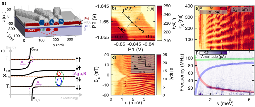
Figure 1: Device operating point and energy spectrum. a) A 3D model of the device, showing a cross section through the double quantum dot region. A full SEM image is shown in Extended Figure E1a. The tunneling to the P1 dot was fast (<100 ns), while loading onto P2 dot is slow (>40 $\mu$s). This asymmetry in tunneling allows latched readout. b) Stability diagram of the (2,8)-(1,9) transition. The labels (N,M) indicate the number of holes in the P1 and P2 dot respectively. The colour scale is sensor current (I_s) in pA, and a full stability diagram down to (0,0) is presented in Extended Data Figure E1b. Zero detuning ($\epsilon=0$) is defined as the (2,8) and (1,9) charge degeneracy point, and positive detuning when the spins are separated into (1,9). Full details of the key points are discussed in the methods. c) Eigenstates calculated using the singlet-triplet Hamiltonian $H_{ST}$ defined in the methods. The coloured arrows indicate the energy transitions observed in the preceding experiments, and $\Delta_{ST}$ indicates the size of the avoided crossing between $\ket{S}$ and $\ket{T_{\pm}}$. Orange dashed lines show how the (1,9) states evolve in absence of spin-orbit coupling. d) The results of a spin funnel experiment with the pulse sequence shown in inset. The spin-funnel experiment was performed by initialising $\ket{S_{2,8}}$, followed by a rapid pulse to a point along the detuning axis ($\epsilon$). At each $B_{x}$ and $\epsilon$ the state was allowed to evolve for a fixed separation time, $\tau_{s}$=100 ns, followed by a pulse to the readout point. The change in sensor signal ($\Delta I$) due to this pulse indicates the likelihood of the returned state being singlet (low $\Delta I$) or triplet (high $\Delta I$) (described in more detail in the methods). Red arrows indicate the $\Delta g$-driven oscillations. e) The same pulse procedure as in d) except the magnetic field is fixed at B_x=5 mT and we investigate the effect of varying the separation time ($\tau_{S}$) at each detuning ($\epsilon$). f) The corresponding FFT at each detuning. Transparent lines indicated the best fit of the observed energy splittings to the eigenstates of $H_{ST}$, and the colours correspond to the transitions indicated in c).

Despite the opportunities holes offer there currently are only limited studies of hole based singlet-triplet qubits. Recently, a hole-spin singlet-triplet qubit was demonstrated in Ge³⁵, where the strong spin-orbit coupling resulted in non-trivial qubit dynamics³⁶. However, the spin-orbit effects in Si devices vary from Ge devices^{37, 38}, therefore similar investigations in silicon would provide valuable understanding of silicon hole-spin effects. Recent experiments in silicon FinFET’s have revealed an anisotropic exchange coupling for holes due to the spin-orbit interaction³⁹, which may provide unique functionalities for hole-spin singlet-triplet qubits. Indeed, theoretical predictions have suggested that the non-trivial relationship between spin-orbit coupling and the site dependent g-tensors may allow hole-spin singlet-triplet qubits to avoid leakage errors³³. However to-date there are no demonstrations of a singlet-triplet qubit using holes in silicon.

In this work we demonstrate a hole-spin singlet-triplet qubit formed in a planar MOS silicon double quantum dot. The planar structure provides a platform suitable for scaling up to the large arrays of coupled qubits needed for quantum circuits and error correction^{40, 41, 42}. Additionally, the planar layout enables the straightforward implementation of a charge sensor. Using this charge sensor, we identify the exact hole occupation of the double dot, which is critical for experimental reproducibility and detailed theoretical modelling of this system. In addition to characterising the key parameters of the qubit, we perform an investigation into the anisotropy of the two-hole eigenstates. By comparing the experimental results with a model that includes spin-orbit coupling and anisotropic site dependent g-tensors, we identify key features in the eigenstates that allow the improvement of the initialisation fidelity and reduction in the readout errors.

Device and operating regime

The hole-spin singlet-triplet qubit is formed using a planar-silicon double quantum dot device, fabricated using industrially compatible CMOS techniques. Figure 1a) shows a model 3D cross section of the double quantum dot region. Multilayer palladium gates define the double quantum dot with P1 and P2 operating as plunger gates, while J_g provides in-situ control of the interdot tunnel coupling $t_{c}$⁴³. The device employs ambipolar charge sensing⁴⁴, with an adjacent $n$MOS SET allowing the absolute charge occupation of each quantum dot to be determined.

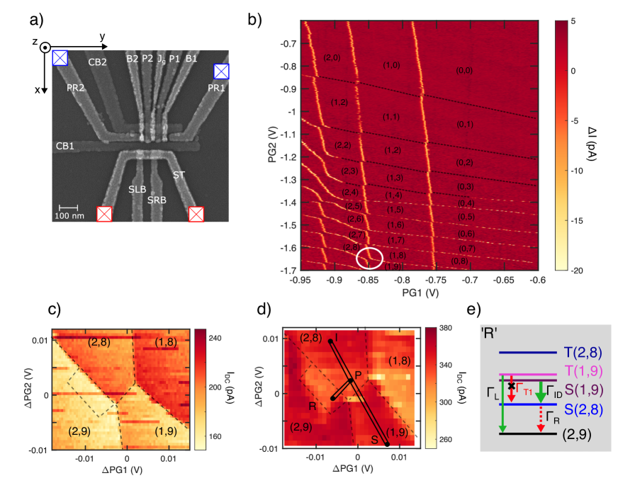
Figure E1: Device and stability diagram. a) SEM image of a nominally identical device that used here. The bottom electrodes (ST, SLB and SRB) are used to form a SET charge sensor, with two n-type ohmics indicated in red. The top electrodes (PR1, B1, P1, $J_{g}$, P2, B2 and PR2) are used to form a double quantum dot, as indicated in Figure1a) of the main text. Gates CB1 and CB2 are used to provide x-axis confinement to the double dot. The hole double quantum dot is connected to two p-type ohmic contacts, indicated by the blue squares. b) Full stability diagram of the device down to the last hole. The colour axis is proportional to $dI/dV_{P1}$, where I is the current through the SET charge sensor. The (2,8)-(1,9) operating point is indicated by the white dashed circle. c) A zoom in of the (2,8)-(1,9) charge stability diagram. The colour scale is the DC sensor current in pA. d) DC sensor current around the (2,8)-(1,9) transition when applying a I-S-P-R (I-S-R) pulse sequence and sweeping the DC voltage on the plunger gates P1 and P2. After initialising at I, pulsing to the S location produces a mix of $\ket{S_{1,9}}$ and $\ket{T_{0}}$. The dwell time at S was chosen to maximise the $\ket{T}$ probability. An enhancement region at the (2,8)-(2,9) transitions allows latched Pauli-spin-blocked readout. This enhancement region is removed when the pulse is reversed (ie M-P-S-R). e) Diagram of the meta-stable states and the expected transitions at the readout position R. the $\ket{T_{0}}$ state is Pauli-spin-blocked from transiting to $\ket{S_{2,8}}$, but can tunnel to the (2,9) ground state at a rate defined by the left dot tunnel rate ($\Gamma_{L}>10$ MHz). $\ket{S_{1,9}}$ will quickly transition to the $\ket{S_{2,8}}$ due to the rapid interdot tunnel rate ($t_{c}>1$ GHz), and will then transition to the (2,9) ground state at a rate defined by the right dot tunnel rate ($\Gamma_{R}<30$ kHz). We used a 20 $\mu$s dwell at the readout point R such that the difference in $\Gamma_{L}$ and $\Gamma_{R}$ allowed readout of $\ket{S_{1,9}}$ and $\ket{T_{0}}$.

Figure 1b) shows a stability diagram measured using the charge sensor. We perform all measurements in the (2,8)-(1,9) configuration, which is equivalent to a (2,0)-(1,1) spin system due to orbital shell filling⁴⁵. We initialised singlet states by dwelling deep in (2,8) where $\ket{S_{(2,8)}}$ is the lowest energy eigenstate (point I). Manipulation of the state was performed by pulsing to a position along the detuning axis ($\epsilon$) and dwelling there for a variable time $\tau_{s}$. Readout of the state was performed by pulsing to point R (following the dashed trajectory), where latched Pauli-Spin-Blockade^{46, 47} readout allowed identification of either the blocked triplet or the unblocked singlet states based on the average sensor current (see methods and Extended Data Figure E1).

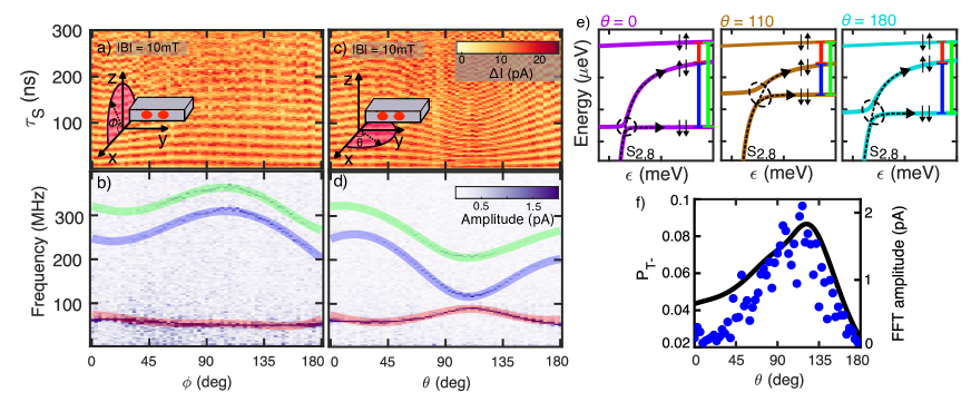
Figure 2: Eigenenergy anisotropy with respect to magnetic field orientation. a-b) Shows the sensor signal and resulting FFT when using the pulse sequence given in Fig 1d) (Initialise-Separate-Readout). Detuning is fixed at $\epsilon$ = 1.9 meV and a 10 mT magnetic field is rotated by 180^∘ through the x-z plane. c-d) Shows the same experiment for a rotation through the sample x-y plane. Transparent solid lines show the optimal fit of $H_{ST}$ to the experimental data. A zoom in of the first 60 ns of c) is shown in Extended Data E2a), highlighting the multiple frequencies present. See Supplement section S2.B for full 360^∘ data set in the x-y plane. e) Shows the eigenenergies for $|B|$ = 10 mT magnetic field is applied at $\theta$ = 0^∘ (purple), 110^∘ (brown), and 180^∘ (cyan) in the x-y plane respectively. The y-axis ticks are in 0.5 $\mu$eV, and x-axis ticks are separated by 1 meV. The energy splitting corresponding to the three FFT peaks in d) are indicated by the red, blue and green vertical lines. The size and location of the $\ket{S}$-$\ket{T_{-}}$ avoided crossing varies with field orientation (black dashed circle), resulting in anisotropy in the Landau-Zener transition probability between $\ket{S_{2,8}}$$\rightarrow$$\ket{T_{-}}$ during the ramp-in/ramp-out. The black dashed lines indicated the splitting of initial state when pulsing across the $\Delta_{ST}$ avoided crossing. f) The solid black line is the calculated probability of the $\ket{S_{2,8}}$ loading into $\ket{T_{-}}$ during the separation pulse ($P_{T_{-}}$, left axis). Blue markers indicate the amplitude of the $\ket{S}$$\leftrightarrow$$\ket{T_{-}}$ FFT peak in d) (transparent blue). Both data are plotted as a function of in-plane magnetic field angle. The trend in $P_{T_{-}}$ correlates with the amplitude of the $\ket{S}$$\leftrightarrow$$\ket{T_{-}}$ oscillations in d). The is correlation between $P_{T_{-}}$ and the $\ket{S}$$\leftrightarrow$$\ket{T_{-}}$ oscillation amplitude is expected since the $\ket{S}$$\leftrightarrow$$\ket{T_{-}}$ oscillations are enhanced as the probability of loading the $\ket{T_{-}}$ state increases.

System Hamiltonian and eigenenergies

To model the two-spin system we consider a 5$\times$5 Hamiltonian, $H_{ST}$, which includes Zeeman, spin-orbit and orbital terms. The full details of the two-hole singlet-triplet Hamiltonian are provided in Supplementary section S1. For the Zeeman Hamiltonian, we include independent 3x3 symmetric g-tensors for the left and right dot, $\mathchoice{\vbox{\halign{#\cr\leftrightarrowfill@{\scriptstyle}\crcr\nointerlineskip\cr$\hfil\displaystyle g\hfil$\crcr}}}{\vbox{\halign{#\cr\leftrightarrowfill@{\scriptstyle}\crcr\nointerlineskip\cr$\hfil\textstyle g\hfil$\crcr}}}{\vbox{\halign{#\cr\leftrightarrowfill@{\scriptscriptstyle}\crcr\nointerlineskip\cr$\hfil\scriptstyle g\hfil$\crcr}}}{\vbox{\halign{#\cr\leftrightarrowfill@{\scriptscriptstyle}\crcr\nointerlineskip\cr$\hfil\scriptscriptstyle g\hfil$\crcr}}}_{L}$ and $\mathchoice{\vbox{\halign{#\cr\leftrightarrowfill@{\scriptstyle}\crcr\nointerlineskip\cr$\hfil\displaystyle g\hfil$\crcr}}}{\vbox{\halign{#\cr\leftrightarrowfill@{\scriptstyle}\crcr\nointerlineskip\cr$\hfil\textstyle g\hfil$\crcr}}}{\vbox{\halign{#\cr\leftrightarrowfill@{\scriptscriptstyle}\crcr\nointerlineskip\cr$\hfil\scriptstyle g\hfil$\crcr}}}{\vbox{\halign{#\cr\leftrightarrowfill@{\scriptscriptstyle}\crcr\nointerlineskip\cr$\hfil\scriptscriptstyle g\hfil$\crcr}}}_{R}$ respectively. Hole-spins in silicon are known to have strongly anisotropic g-tensors^{24, 26, 39}, where variations in the g-tensor are produced by non-uniform strain^{26, 48}, spin-orbit coupling⁴⁹ and differences in the confinement profile between the two dots⁵⁰. Hence, we do not assume that $\mathchoice{\vbox{\halign{#\cr\leftrightarrowfill@{\scriptstyle}\crcr\nointerlineskip\cr$\hfil\displaystyle g\hfil$\crcr}}}{\vbox{\halign{#\cr\leftrightarrowfill@{\scriptstyle}\crcr\nointerlineskip\cr$\hfil\textstyle g\hfil$\crcr}}}{\vbox{\halign{#\cr\leftrightarrowfill@{\scriptscriptstyle}\crcr\nointerlineskip\cr$\hfil\scriptstyle g\hfil$\crcr}}}{\vbox{\halign{#\cr\leftrightarrowfill@{\scriptscriptstyle}\crcr\nointerlineskip\cr$\hfil\scriptscriptstyle g\hfil$\crcr}}}_{L}$ and $\mathchoice{\vbox{\halign{#\cr\leftrightarrowfill@{\scriptstyle}\crcr\nointerlineskip\cr$\hfil\displaystyle g\hfil$\crcr}}}{\vbox{\halign{#\cr\leftrightarrowfill@{\scriptstyle}\crcr\nointerlineskip\cr$\hfil\textstyle g\hfil$\crcr}}}{\vbox{\halign{#\cr\leftrightarrowfill@{\scriptscriptstyle}\crcr\nointerlineskip\cr$\hfil\scriptstyle g\hfil$\crcr}}}{\vbox{\halign{#\cr\leftrightarrowfill@{\scriptscriptstyle}\crcr\nointerlineskip\cr$\hfil\scriptscriptstyle g\hfil$\crcr}}}_{R}$ are correlated or share the same principle spin-axes. For the spin-orbit Hamiltonian we include a spin-orbit vector, $\vec{t}_{so}=(t_{x},t_{y},t_{z})$, parameterising the effect of spin-orbit coupling in the laboratory reference frame indicated in Figure 1a).

In Figure 1c) we plot the eigenenergies of $H_{ST}$ as a function of detuning. At negative detuning the eigenstates are the ($\ket{T_{+}},\ket{T_{0}},\ket{T_{-}},\ket{S},\ket{S_{(2,8)}}$) basis states. At large positive detuning the eigenstates evolve into the $\ket{S_{2,8}}$ state and the four two-spin states ($\ket{\uparrow\uparrow},\ket{\uparrow\downarrow},\ket{\downarrow\uparrow},\ket{\downarrow\downarrow}$), which are defined by the sum or difference of the Zeeman energy in the two dots. The $\ket{\uparrow\downarrow}$ and $\ket{\downarrow\uparrow}$ eigenstates have energy splitting given by

$$E_{ST_{0}} =\sqrt{J(\epsilon,t_{c})^{2}+\Delta E_{z}^{2}}$$ (1)

where

$$J(\epsilon) =\sqrt{\frac{\epsilon^{2}}{4}+2t_{c}^{2}}-\frac{\epsilon}{2}$$

$$\Delta E_{z} =|\Delta g^{*}|\mu_{B}|\vec{B}|$$

$\epsilon$ is the detuning energy, $t_{c}$ is the interdot tunnel coupling, $\Delta g^{*}$ is the difference in the effective g-factors for the applied magnetic field vector $\vec{B}$ (see Supplement S1), and $\mu_{B}$ is the Bohr magneton. Since strong spin-orbit coupling results in an anisotropy in $|\Delta g^{*}|$ with respect to magnetic field orientation, we expect $E_{ST_{0}}$ to exhibit a non-trivial anisotropy³⁹. An avoided crossing occurs between the $\ket{S_{2,8}}$ and $\ket{T_{\pm}}$, with the amplitude of the avoided crossing ($\Delta_{ST_{\pm}}$) determined by the interplay between the spin-orbit vector and the difference in the projection of the g-tensors for the given field orientation³⁶.

Figure 1d) shows the charge sensor response of a spin-funnel experiment used to characterise the singlet-triplet system⁵. The spin-funnel experiment was performed by allowing a singlet state to time-evolve for $\tau_{s}$ = 100 ns at each $B_{x}$ and $\epsilon$. The change in sensor signal ($\Delta I$) then measures the likelihood that the final state is either singlet (low $\Delta I$) or triplet (high $\Delta I$). A clear funnel edge is visible in $\Delta I$ when the detuning point coincides with the $\ket{S}$ and $\ket{T_{\pm}}$ avoided crossing⁵. In addition, on the positive detuning side of the funnel edge we see oscillations that result from $\Delta g$-driven $\ket{S}$$\leftrightarrow$$\ket{T_{0}}$ oscillations (red arrows).

Figure 1e) we demonstrate the time evolution of the singlet at each detuning. The experimental procedure is the same as Figure 1d), however here we varied the separation time ($\tau_{S}$) at each detuning ($\epsilon$) and held the magnetic field constant at $B_{x}$ = 5 mT. Figure 1f) shows the FFT of $\Delta I$ at each $\epsilon$, revealing three clear oscillation frequencies, each with a distinct detuning dependence. Each oscillation frequency results from mixing between the three lowest eigenstates at the separation detuning ($\epsilon$). The lowest frequency (red) results from oscillations between $\ket{S}$$\leftrightarrow$$\ket{T_{0}}$ states, the middle frequency (blue) results from oscillations between $\ket{S}$$\leftrightarrow$$\ket{T_{\pm}}$, and the highest frequency (green) results from oscillations between $\ket{T_{0}}$$\leftrightarrow$$\ket{T_{\pm}}$. The corresponding transitions are indicated by coloured arrows in Figure 1c) and a full description is provided in the methods.

We fit the observed frequencies in Figure 1f) to the eigenergies of the singlet-triplet Hamiltonian, $H_{ST}$ and extract key parameters of the two-hole system. Transparent lines in Figure 1f) show the best fit, demonstrating good agreement between the observed and theoretical eigenenergies. Based on the best fit we extract $t_{c}=9\pm 1$ $\mu$eV and two effective g-factors of $0.8\pm 0.1$ and $1.2\pm 0.1$ for $B_{x}$.

Anisotropic g-tensors and spin-orbit coupling

To characterise the key parameters of the two-hole system we investigate the effect of magnetic field orientation on the two-hole eigenenergies. Figure 2a) shows $\Delta I$ as a function of $\tau_{S}$ for a range of magnetic field orientations in the x-z plane and Figure 2b) shows the resulting FFT of $\Delta I$. Figures 2c-d) repeat the same experiment for a rotation of the magnetic field through the x-y plane. Clear anisotropy with respect to magnetic field orientation can be observed, which results from the interplay between spin-orbit coupling and the orientation of the g-tensors. The visibility of the higher frequency (blue and green) oscillations also shows a strong dependence on the magnetic field orientation. In particular, the FFT amplitude of the higher frequency (blue and green) oscillations is suppressed for $B_{x}$ and enhanced for $B_{y}$ and $B_{z}$.

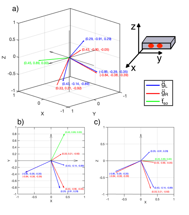
Figure E4: Fitting parameters for the g-tensors and spin orbit vector. a) The principle axes of the optimal $\mathchoice{\vbox{\halign{#\cr\leftrightarrowfill@{\scriptstyle}\crcr\nointerlineskip\cr$\hfil\displaystyle g\hfil$\crcr}}}{\vbox{\halign{#\cr\leftrightarrowfill@{\scriptstyle}\crcr\nointerlineskip\cr$\hfil\textstyle g\hfil$\crcr}}}{\vbox{\halign{#\cr\leftrightarrowfill@{\scriptscriptstyle}\crcr\nointerlineskip\cr$\hfil\scriptstyle g\hfil$\crcr}}}{\vbox{\halign{#\cr\leftrightarrowfill@{\scriptscriptstyle}\crcr\nointerlineskip\cr$\hfil\scriptscriptstyle g\hfil$\crcr}}}_{L}$ (blue) and $\mathchoice{\vbox{\halign{#\cr\leftrightarrowfill@{\scriptstyle}\crcr\nointerlineskip\cr$\hfil\displaystyle g\hfil$\crcr}}}{\vbox{\halign{#\cr\leftrightarrowfill@{\scriptstyle}\crcr\nointerlineskip\cr$\hfil\textstyle g\hfil$\crcr}}}{\vbox{\halign{#\cr\leftrightarrowfill@{\scriptscriptstyle}\crcr\nointerlineskip\cr$\hfil\scriptstyle g\hfil$\crcr}}}{\vbox{\halign{#\cr\leftrightarrowfill@{\scriptscriptstyle}\crcr\nointerlineskip\cr$\hfil\scriptscriptstyle g\hfil$\crcr}}}_{R}$ (red) are indicated as normalised vectors in the x-y-z plane. The full g-tensors are presented in the methods section. There is a clear misalignment between the principle axes of the left and right g-tensors. The spin-orbit vector is plotted in green. Normalised vectors are used to compare orientations of each g-tensor and the spin-orbit vector, and the components of each normalised vector are indicated. b) and c) show 2D projections of a) in the x-y plane and the x-z plane respectively.

The 3x3 g-tensors for each dot and the spin-orbit orientation can be extracted by fitting the data in Figure 2a-d) to the eigenenergies of $H_{ST}$. The fitting procedure is discussed in Supplementary sections S3-S5. The transparent lines in Figures 2b) and d) indicate the frequency of the respective FFT peaks for the optimal fit parameters. For the optimal fit we find ($t^{x}_{so},t^{y}_{so},t^{z}_{so}$) = ($-37~{}\pm~{}2,107~{}\pm~{}4,0~{}\pm~{}20$) neV, giving $|\vec{t}_{so}|$ = 0.12 $\mu$eV. Notably, $\vec{t}_{so}$ is oriented in-plane with the 2DHG, consistent with expectations for heavy holes in planar silicon⁵¹. Further, the in plane spin-orbit vector has components in both $t^{x}_{so}$ and $t^{y}_{so}$, indicating that a combination of Rashba (oriented perpendicular to the double dot axis) and Dresselhaus (oriented parallel to the double dot axis) spin-orbit components are present⁵². The full g-tensors are presented in the Extended Data Figure E4. We find that the orientation of the g-tensor principle axes for left and right dots are slightly misaligned, which may result from differences in confinement profile or non-uniform strain between the left and right dot. The observation of misalignment in the g-tensor principle axes suggests accurate modelling of multiple quantum dot systems in silicon should incorporate site dependent g-tensors with differing principle axes.

The anisotropy in the FFT amplitudes in Figure 2a-d) is caused by the probability of transitioning from $\ket{S_{2,8}}$ into $\ket{T_{-}}$ during the pulse from (2,8) to (1,9). When pulsing from (2,8) to (1,9) the $\Delta_{ST_{\pm}}$ avoided crossing causes the initial $\ket{S_{2,8}}$ state to be split between $\ket{S}$ and $\ket{T_{-}}$ with a ratio determined by the Landau-Zener transition probability⁵³ (see methods). Larger $\Delta_{ST_{\pm}}$ favours $\ket{T_{-}}$ states, while smaller $\Delta_{ST_{\pm}}$ favours $\ket{S}$. In Figure 2e) we plot the energy spectrum of the two-hole system for various in-plane magnetic field orientations. The magnetic field orientation strongly influences the magnitude of $\Delta_{ST_{\pm}}$ and the position in detuning ($\epsilon_{\Delta}$) at which the avoided-crossing occurs. As a result, the magnetic field orientation impacts the likelyhood of populating the $\ket{T_{-}}$ state during the separation ramp and thus impacts the amplitude of the $\ket{S}$$\leftrightarrow$$\ket{T_{-}}$ FFT peak.

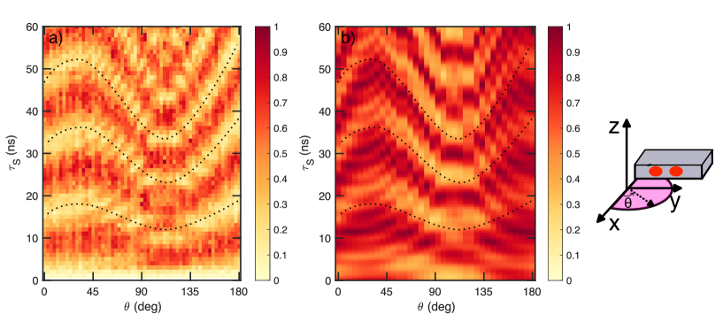
Figure E2: Zoom in of Figure 2 and comparison with QuTip Simulation. a) The experimental data from Figure 2c) is reproduced over a shortened time scale. The colour scale is the normalised singlet probability. Black dashed lines serve as a guide to the eye for the anisotropy in the period of the $\Delta$g-oscillations. At $\theta$=0 the slower $\ket{S}$$\leftrightarrow$$\ket{T_{0}}$ oscillations are the main component picked up in the FFT data of Figure 2d). However as $\theta$ increases additional spectral components become more pronounced, with most significant effects observed at $\theta$ = 120^∘. These additional spectral components arise from both $\ket{S}$$\leftrightarrow$$\ket{T_{\pm}}$ oscillations and $\ket{T_{0}}$$\leftrightarrow$$\ket{T_{\pm}}$, which both become more prevalent as $\Delta_{ST}$ becomes both more open and moves to more positive detuning (See Figure 2e). d) Shows the full simulation of the experimental procedure using the Qutip code and model described in Supplementary sections S1, S3 and S4. The black dashed lines are transposed from a) to show that the simulation captures the key experimentally observed features. We note that the experiment in a) takes approximately 3hrs to perform and is limited by the integration time of the SRS830 lock-in (0.3ms). The simulation in b), which uses QuTip ‘sesolve’ function, takes approximately 10 hrs to run, and is limited by the number of PC cores running simultaneously.

We simulated the experimental pulse sequence using QuTiP⁵⁴ and calculated the $\ket{S_{2,8}}$$\rightarrow$$\ket{T_{-}}$ transition probability ($P_{T_{-}}$), which yielded good agreement with the measured FFT amplitude. In Figure 2f), the solid line shows the calculated $P_{T_{-}}$ using the optimal fit parameters for a range of in-plane magnetic field orientations (See Supplement section S3 for details). The circles in Figure 2f) show the observed amplitudes of the $\ket{S}$$\leftrightarrow$$\ket{T_{-}}$ FFT peaks from Figure 2d) (blue). The trend in $P_{T_{-}}$ matches the anisotropy in the measured amplitudes of the $\ket{S}$$\leftrightarrow$$\ket{T_{-}}$ FFT peaks from Figure 2d), with both exhibiting a peak around $\theta$ = 120^∘, and an asymmetric reduction towards 0^∘ and 180^∘. The correlation between FFT amplitude and the calculated $P_{T_{-}}$ demonstrates that the model $H_{ST}$ and optimal fit parameters captures the dynamics of the hole-spin qubit well (See Extended Data Figure E2a).

We now consider how hole-spin singlet-triplet qubits can be further optimised by using the anisotropic response of the system to a magnetic field. For the singlet-triplet qubit studied here, optimal initialisation protocol would suppress the likelyhood of the $\ket{S_{2,8}}$ state loading into the $\ket{T_{-}}$ leakage state. In the presence of large spin-orbit coupling and/or large $\Delta g$, even rapid separation pulses may be unable to satisfy the non-adiabatic Landau-Zener requirement imposed by the large $\Delta_{ST_{-}}$ avoided crossing. However, with knowledge of the orientation of spin-orbit vector ($\vec{t}_{so}$), and the g-tensors, we can identify optimum field orientations to minimise $\Delta_{ST_{-}}$ and thus enhance initialisation fidelity. Indeed, in Figure 2f) we have shown that the B_x magnetic field suppress loading into the $\ket{T_{-}}$ state, and therefore is an optimal field orientation for the singlet-triplet qubit in this system.

Coherent $\Delta$g-driven oscillations

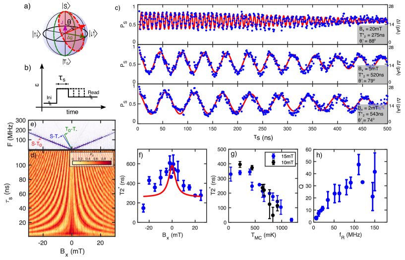
Figure 3: $\Delta g$-driven coherent oscillations. a) Shows a schematic of the Bloch sphere for the singlet-triplet qubit. The Zeeman energy difference $\Delta E_{z}$ produces oscillations about the x-axis ($\ket{S}$$\leftrightarrow$$\ket{T_{0}}$ oscillations), while exchange coupling $J$ produces oscillations about the z-axis (ie $\ket{\uparrow\downarrow}$$\leftrightarrow$$\ket{\downarrow\uparrow}$ oscillations). When both $J$ and $\Delta E_{z}$ are non-zero, the angle of rotation with respect to the Bloch sphere z-axis is given by $\theta^{\prime}$ = arctan$(\frac{\Delta E_{z}}{J})$ as indicated by the red trajectory. b) Shows the pulse sequence used to drive the $\Delta g$-driven oscillations. We initialised in $\ket{S_{2,8}}$, then applied a rapid separation pulse along the detuning axis. The system was then held at a fixed positive detuning ($\epsilon$) for a separation time ($\tau_{S}$), before performing readout. c) Shows the observed $\ket{S}$$\leftrightarrow$$\ket{T_{0}}$ oscillations as a function of separation time, for $B_{x}$ = 20 mT, 5 mT and 2 mT. The solid red line is the best fit of Eqn. 3 to the data. The singlet probability, $P_{S}$, at each $\tau_{S}$ is extracted from the change in the normalised sensor signal $\Delta I$ (shown on right axis, see methods for full details). d) Shows the $\ket{S}$$\leftrightarrow$$\ket{T_{0}}$ oscillations over a field range of $B_{x}$ = $\pm$30 mT. e) Shows the FFT of the oscillations observed in d). A linear increase in the oscillation frequency is expected since $hf$ = $\Delta E_{ST_{0}}$ (Eqn. 1). The $B_{x}$ magnetic field orientation was used for these experiments since it results in the least leakage into $\ket{T_{-}}$ (Figure 2). However, residual loading of the $\ket{T_{-}}$ leakage state results in weak $\ket{S}$$\leftrightarrow$$\ket{T_{-}}$ (blue) and $\ket{T_{0}}$$\leftrightarrow$$\ket{T_{-}}$ (green) oscillations for $B_{x}$. f) Shows the $T2^{*}$ for different magnetic fields, where the solid line is the best fit of Eqn. 4 to both this data and the data in Figure 4e). g) Shows the effect of mixing chamber temperature on $T_{2}^{*}$ for two different magnetic fields. h) The qubit quality factor ($Q$) as a function of the $\Delta$g-driven oscillation frequency ($f_{R}$), measured at $T_{MC}$=30 mK. All data in Figure 3 was collected with $J_{g}$ = 1.2 V.

We now turn to experiments to characterise the hole-spin qubit. Here, the qubit is defined using the $\ket{S}$ and $\ket{T_{0}}$ states of the double quantum dot. The simplified Hamiltonian for this system can be written as

$$H_{ST}=\frac{J}{2}\sigma_{z}+\frac{\Delta E_{z}}{2}\sigma_{x}$$ (2)

where $J$ defines the exchange energy, $\Delta E_{z}=|\Delta g^{*}|\mu_{B}|B|$, $|B|$ is the magnitude of the applied field, $\sigma_{x,z}$ are the respective Pauli matricies and $\mu_{B}$ is the Bohr magneton. The Bloch sphere for this qubit system is shown in Figure 3a). Rotations around the Bloch sphere can be driven by controlling $J$ and $\Delta E_{z}$ at the separation point^{55, 7}, and Figure 3b) shows a schematic of the pulse sequence used.

Figure 3c) plots the measured singlet probability $P_{S}$ as a function of separation time $\tau_{S}$ for three different |$B_{x}$|, demonstrating oscillations in $P_{S}$. Solid lines in Figure 3b) show the best fit of the data to the equation

$$P_{S}=A\text{cos}(2\pi f_{R}\tau_{s}+\phi)\text{Exp}[(\frac{\tau_{s}}{T^{*}_{2}})^{\alpha}]+C$$ (3)

where $f_{R}$ is the Rabi frequency, $\tau_{s}$ is the separation time, $\phi$ is a phase offset, $T_{2}^{*}$ is the qubit dephasing time, A is the oscillation amplitude, C is an offset, and $\alpha$ captures the noise colour (see Supplementary section S2.A).

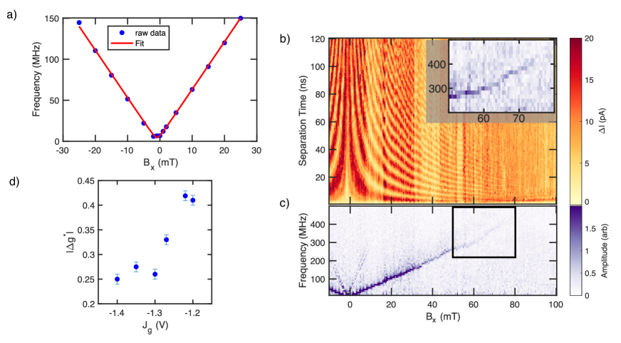
Figure E3: Additional analysis of singlet-triplet oscillations. a) The singlet-triplet oscillation frequency is plotted as a function of the in-plane magnetic field $B_{x}$. The solid red line shows the best fit of the raw data to Eqn. 1. From the fit we extract the |$\Delta g*$| for this field orientation, and the residual exchange coupling $J$. b) Shows singlet-triplet oscillations for an in-plane magnetic field up to $B_{x}$=100 mT. c) The FFT at each |$B_{x}$| from b) shows the frequency of the singlet-triplet oscillations. A zoom-in of the black rectangle are is shown as in the inset of b), revealing that singlet-triplet oscillations persist to 400 MHz. d) Shows the extracted $\Delta g$ as a function of the $J_{g}$ gate voltage, demonstrating in-situ control of $\Delta g$.

Analysis of the $\ket{S}$$\leftrightarrow$$\ket{T_{0}}$ oscillations over a range of $B_{x}$ was used to characterise the qubit control frequency ($f_{R}$) and the coherence time ($T^{*}_{2}$). Figures 3d) and e) show a colour map of the $\ket{S}$$\leftrightarrow$$\ket{T_{0}}$ oscillations and a corresponding FFT at each $B_{x}$. We resolve $\ket{S}$$\leftrightarrow$$\ket{T_{0}}$ oscillations up to 150 MHz at 30 mT and have observed up to 400 MHz at 80 mT (Extended data Figure E3). To extract $\Delta g$ and $J$ we fit $f_{R}$ for each $B_{x}$ to Eqn. 1. The fit yields $J$ = 6 MHz at the separation point ($\epsilon=1.9$ meV), and $|\Delta g|$ = 0.41 which is in agreement with the effective g-factors extracted from Figure 1f. In Extended data Figure E3d) we show electrical control over $\Delta g^{*}$ using the $J_{g}$ gate, with a trend of $d\Delta g^{*}/dJ_{g}\approx$ 0.9 V^-1, demonstrating in-situ electrical control of the qubit control frequency.

We now show the decoherence in this qubit can be explained by fluctuations in both $\epsilon$ and $\Delta E_{Z}$ and we quantify their magnitudes. Figure 3f) shows $T_{2}^{*}$ for a range of $B_{x}$, where each $T_{2}^{*}$ has been extracted using a fit to Eqn 3. Dephasing is caused by fluctuations in the energy splitting between the $\ket{S}$ and $\ket{T_{0}}$ states⁵⁶ (Eqn 1). Hence, the variation in $T_{2}^{*}$ can be modelled using

$$\frac{1}{T_{2}^{*}}=\frac{\pi\sqrt{2}}{h}\sqrt{(\frac{J}{E_{ST_{0}}}\frac{dJ}{d\epsilon}\delta\epsilon)^{2}+(\frac{\Delta E_{Z}}{E_{ST}}\delta\Delta E_{Z})^{2}}$$ (4)

where $\delta\epsilon$ is the noise in detuning and $\delta\Delta E_{Z}$ is the effective magnetic noise. A common fit of the data in Figures 3f) and 4d) (discussed later) was used to extract $\delta\epsilon~{}=~{}30~{}\mu$eV and $\Delta E_{Z}=4$ neV. These values are comparable to those previously reported for electrons in silicon micro-magnet devices⁵⁷ and for holes in planar Ge devices³⁵. The similarity in $\delta\epsilon$ between holes in planar Si and planar Ge suggests that the highly disordered SiO₂ oxide does not significantly enhance the effect of charge noise compared to planar Ge heterostructures, where the quantum dot is buried tens of nanometers below the surface. Further, the similarity in $\delta\epsilon$ between this work in $p$MOS silicon and studies of electrons in $n$MOS silicon⁵⁷ suggests that the level of charge noise is not impacted by the polarity of the gate bias.

In Figure 3g) we plot $T_{2}^{*}$ of the $\Delta$g-driven oscillations as a function of the fridge mixing chamber temperature ($T_{MC}$). $T_{2}^{*}$ is approximately independent of $T_{MC}$ up to 400 mK ($k_{B}T=34$ $\mu$eV ), where $T_{2}^{*}$ begins to drop. The $T_{2}^{*}$ behaviour shows the same trend at $B_{x}$ = 15 mT ($\Delta E_{ST_{0}}=0.35$ $~{}\mu$eV) and $B_{x}$ = 10 mT ($\Delta E_{ST_{0}}=0.23$ $\mu$eV). Interestingly, we find that the noise colour ($\alpha$) appears to whiten as the temperature of the fridge increases, consistent with recent experiments in other hole spin qubits²⁰ (see Supplement section S2.A).

Finally, in Figure 3h) we show that the quality factor ($Q=f_{R}\times T_{2}^{*}$) of the $\Delta$g-driven singlet-triplet oscillations increases as the control speed increases. The quality factor quantifies the number of coherent oscillations that can be completed within the coherence time. A promising feature of this qubit is that Q increases with increasing $f_{R}$, indicating that the qubit control speed can be increased without degrading the quality.

Coherent exchange-driven oscillations

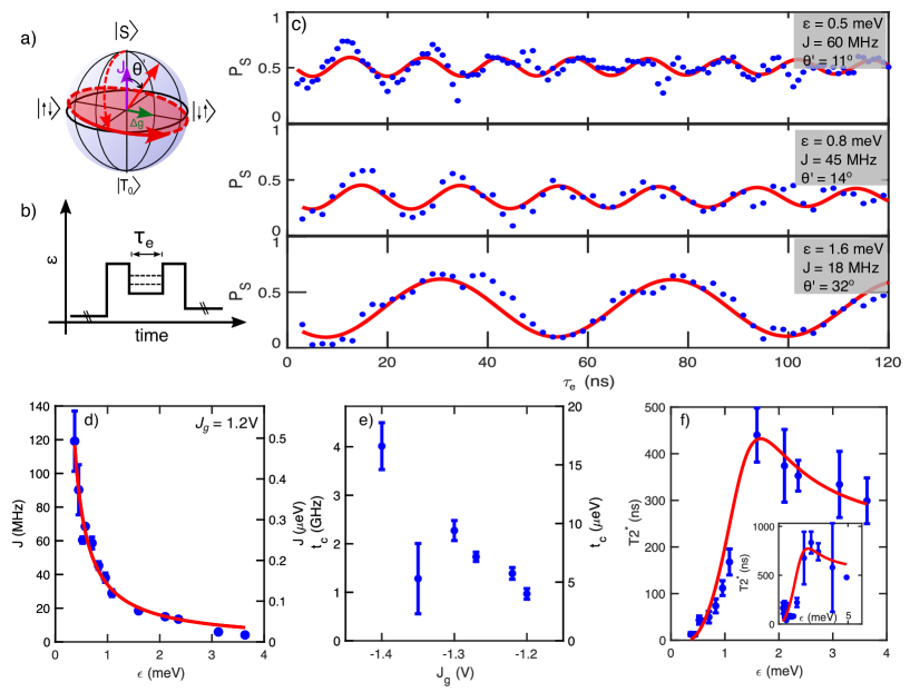
Figure 4: Exchange-driven coherent oscillations. a) A schematic of the state evolution and b) shows the pulse sequence used to achieve exchange-driven oscillations. A $\Delta g$-driven $\pi/2$ pulse brings the qubit to the equator (red dashed trajectory), then a rapid pulse to low detuning is used to suddenly increase J, changing the angle of rotation, resulting in exchange-driven oscillations around the equator (red trajectory). The orientation of the oscillation is tilted by $\theta^{\prime}$ from the z-axis. c) Exchange-driven oscillations for three different detunings ($\epsilon$= 0.5 meV, 0.8 meV, and 1.6 meV). Experiments were performed with a fixed magnetic field of B_x = 2 mT, such that a $\Delta g$-driven $\pi/2$ pulse takes 65ns. The solid line shows a best fit to Eqn. 3, allowing extraction of J and $T_{2}^{*}$ at each $\epsilon$. d) Exchange energy as a function of detuning, measured using the exchange pulse. The solid red lines shows the fit to $J(\epsilon,t_{c})=\sqrt{\frac{\epsilon^{2}}{4}+2t_{c}^{2}}-\frac{\epsilon}{2}$, allowing the extraction of the tunnel coupling $t_{c}$. e) Tunnel coupling extracted for a range of different $J_{g}$ gate voltages, where each $t_{c}$ is extracted from the $\epsilon$ dependence of the exchange-oscillation frequency. f) Dephasing time $T_{2}^{*}$ as a function of the detuning. The solid red line is a joint fit of Eqn. 4 to this data and the data in Figure 3f). All data in c), d) and f) was collected for $J_{g}$ = 1.2 V, and the inset in f) shows the dephasing time as a function of the detuning for J_g = -1.4 V.

In order to achieve full control of the singlet-triplet qubit it is necessary to produce control pulses around two orthogonal axes of the Bloch sphere. We use exchange-driven oscillations to rotate the qubit around the z-axis of the Bloch sphere. By combining $\Delta g$-driven (x-axis) and exchange-driven (z-axis) rotations, it is possible to achieve full control over the qubit Bloch sphere.

Figures 4a) and 4b) show the experimental procedure for exchange-driven oscillations. A separation pulse with calibrated $\tau_{S}$ is first used to perform a $\Delta g$-driven $\frac{\pi}{2}$ rotation to bring the state to the equator of the Bloch sphere. A rapid pulse to low detuning is then applied, which suddenly increases J, producing a change in qubit rotation axis. The system is held at the exchange-point for $\tau_{E}$ to drive oscillations around the z-axis, then a second $\Delta g$-driven $\frac{\pi}{2}$ rotation is applied, followed by a pulse to the readout position.

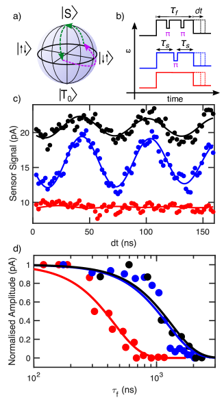
Figure 5: Spin echo measurement at $B_{x}$ = 1.6 mT. a) Shows an example trajectory of the qubit-state for the refocusing pulse schematic of b). Free evolution driven by $\Delta g$ is allowed for a period of time $\tau_{S}(n)=(2n+1/2)t_{\pi}$ (green trajectory), such that after any $\tau_{S}(n)$ the qubit will be at the equator. A refocusing pulse is incorporated as a $\pi$ exchange pulse, followed by a second period of free evolution for $\tau_{S}(n)$. The total time to perform this sequence is the free evolution time, $\tau_{f}$, which can be varied by increasing $n$, or repeating the cycle to include multiple refocusing pulses. The full pulse sequence results in the qubit refocusing to $\ket{S}$ after $\tau_{f}$. c) Residual $\ket{S}-\ket{T_{0}}$ oscillations after a free evolution time ($\tau_{f}$) of 1000 ns for no refocusing pulses (red), one refocusing pulse (blue) and two refocusing pulses (black). d) Normalised peak-to-peak amplitude of the residual $\ket{S}-\ket{T_{0}}$ oscillations as a function of free evolution time. For one (blue) and two (black) refocusing pulses the oscillations are clearly extended compared with the data for no refocusing pulse. The amplitude is normalised against the shortest free evolution for each data set in order to account for the fidelity of the $\pi$ exchange pulse. We extract $T^{*}_{Echo}$ based on a fit to the decay envelope of Eqn. 4, using $\alpha=2$ (see Supplement section S2.A). The experiments were performed for $B_{x}$ = 1.6 mT.

Figure 4c) demonstrates exchange-driven oscillations at three different detuning position ($\epsilon$). Reducing $\epsilon$ at the exchange position increases the exchange energy J, so that the angle of rotation tends towards 0^∘ with respect to the Bloch sphere z-axis (since J $\gg\Delta g\mu_{B}B$). In Figure 4d) we plot $J$ as a function of $\epsilon$ at the exchange point. The solid line shows the best fit of $J(\epsilon,t_{c})$, allowing the extraction of the tunnel coupling (see Figure caption). This experiment was repeated for a range of $J_{g}$ gate voltages, and the resulting dependence of the tunnel coupling ($t_{c}$) on the $J_{g}$ gate voltage is shown in Figure 4e), demonstrating smooth control of $t_{c}$. Therefore, the exchange-driven oscillations are highly tunable, since $J$ can be electrically tuned either by varying $\epsilon$ with the plunger gates, or by tuning $t_{c}$ using the $J_{g}$-gate. These results demonstrate coherent exchange-driven z-axis control of the singlet-triplet qubit.

Figure 4f) presents $T^{*}_{2}$ as a function of $\epsilon$, which is used to characterise the coherence time of the exchange oscillations. The solid line shows the best fit to Eqn. 4, obtained by jointly fitting Figure 4e) and Figure 3f). The trend in $T^{*}_{2}$ is well explained by Eqn. 4, where charge noise ($\delta\epsilon$) dominates at low detuning due to enhanced $dJ/d\epsilon$, while Zeeman noise ($\delta\Delta E_{Z}$) dominates at large detuning where $dJ/d\epsilon\xrightarrow{}0$.

Spin echo measurement

Finally, we investigate the use of spin-refocusing to enhance the qubit coherence time. Given that J and $\Delta E_{Z}$ are non-zero, rotations around the Bloch sphere occur at some angle offset from the pure x-axis or z-axis. Since the qubit trajectory is not solely around the x-axis or z-axis, the precise form of the refocusing pulse will vary as the qubit evolves. Therefore, complicated pulse engineering is required for perfect refocusing pulses⁵⁸. Here, we implement a simplified procedure³⁵, which employs a $\pi$ rotation using an exchange pulse to enhance the observed coherence analogous to a Hahn echo. Figures 5a) and b) show the qubit evolution and pulse sequence for the refocusing procedure respectively. The spin echo experiment allowed the qubit to freely evolve for a time $t_{f}$, during which $N$ exchange-driven $\pi$ rotations are carefully interlaced to provide the refocusing echo. Full details of the refocusing procedure are provided in the methods.

We demonstrate the enhancement of the qubit coherence by observing the residual $\Delta g$-driven singlet-triplet oscillations after the free evolution time, $t_{f}$. Figure 5c) shows the singlet-triplet oscillations after $t_{f}$ = 1000 ns for zero (red), one (blue) and two (black) refocusing pulses. When zero refocusing pulses are applied the singlet-triplet oscillations are completely lost after 1000 ns of free evolution. However, with refocusing pulses the singlet-triplet oscillations are visible even after $t_{f}>1000$ ns. Figure 5d) shows the normalised amplitude of the residual $\Delta g$-driven singlet-triplet oscillations observed for a range of free evolution times. The application of one and two refocusing pulses clearly enhances the coherence of the qubit. We fit the decay of the peak amplitude to extract $T^{Echo}_{2}$ = 1220$\pm$150 ns for one refocusing pulse, and $T^{Echo}_{2}$ = 1300$\pm$200 ns for two refocusing pulses. When no refocusing pulses are applied we find $T^{Echo}_{2}$ = 550$\pm$50 ns, consistent with the measurements in Figure 3. Although we see an improvement of 120% by applying one pulse, we see no significant improvement when using two refocusing pulses. This suggests the maximum $T^{Echo}_{2}$ may have been reached for this simplified refocusing procedure.

Conclusion

In this work we have demonstrated a hole-spin singlet-triplet qubit in planar silicon. We demonstrate rapid $\ket{S}$$\leftrightarrow$$\ket{T_{0}}$ oscillations exceeding 400 MHz, two axis control via $\Delta g$-driven and exchange-driven oscillations, and enhancement of the qubit coherence time to >1 $\mu$s using spin-echo procedures. Developing a complete model of the energy spectrum provided insight into spin-qubit dynamics under rapid pulses across the $\ket{S}$$\leftrightarrow$$\ket{T_{-}}$ avoided crossing. The experimentally observed effects were well described by the model Hamiltonian, providing insight into methods to further optimise initialisation protocols in hole-spin qubits.

Methods

Sample details

The device was fabricated from high resistivity natural silicon. A SEM image of a nominally identical device is shown in Figure E1a) where the multi-layer Pd gate stack is achieved using 2nm ALD AL₂O₂ and a high quality 5.9nm SiO₂ gate oxide. This device combines nMOS and pMOS capabilities in order to implement a Single Electron Transistor (SET) as the charge sensor, while defining a hole double quantum dot^{44, 43}.

Device operation

A Single Electron Transistor (SET) was defined by the ST (Sensor Top gate) and the left and right barrier gates (SLB and SRB)⁵⁹. A double quantum dot was formed by carefully biasing the gates B1, P1, J_g, P2, and B2. Gates PR1 and PR2 were used to accumulate a 2D hole gas, which served as a reservoir of holes. In addition to providing confinement, the B1 and B2 gates can also modulate the tunneling rate between the hole quantum dots and the reservoirs. In this experiment we asymmetrically biased B1 and B2 (B1 = -0.6V, B2 = -0.4V). Configuring different lead-dot tunnel rates between the left and right dot enabled latched readout, which is discussed later.

The SET acts as a highly sensitive charge sensor for the adjacent hole double quantum dot. In Figure E1b) we show a large stability diagram of the double quantum dot, measured by applying a small (1mV) pulse at 177Hz on P1 and monitoring the the charge sensor using a lock-in reference to this pulse⁴⁵. In addition, dynamic feedback is used to maintain the SET at a sensitive position over the large range of plunger gates used⁶⁰. The use of a charge sensor allows confirmation of the absolute hole occupation since the (0,0) region can be identified. We note that some transitions lose visibility (black dashed lines) since the tunnel rate becomes slower than the 177Hz used for the measurement. However all transitions can be inferred by the observation of avoided inter-dot transitions. The (2,8)-(1,9) region used in this experiment is indicated by a white circle.

Experimental Setup

All experiments were performed using a top loading BlueFors XLD dilution fridge with a 3-axis vector magnet. Unless otherwise stated the experiments were performed with the fridge at base temperature where the mixing chamber thermometer was 40 mK. Previous measurements indicated that at base this system achieves electron and hole temperatures of 120 mK. The device was fixed directly onto a brass sample enclosure that is thermally anchored to the probe cold-finger. GE varnish was used to mount the device directly onto a brass sample stage, and Al bond wires connect the sample to a home-made printed circuit board. All DC biasing was applied using a Delft IVVI digital-to-analogue-converter using lines which each pass through individual 50kHz low pass filters mounted to the cold finger (40 mK). The current through the SET was amplified using a Basel SP983c I-V preamplifier. DC currents were then monitored using a Keithly 2000, and standard low-frequency lock-in techniques were implemented using a SR830.

Rapid pulses were applied to gates P1 and P2 in order to perform initialisation, control and readout out of the singlet-triplet qubit. The pulses were applied using a Tabor WX1284 with 1.25 GS/s. Fast pulses from the WX1284 were routed to gates P1 and P2 using homemade RC bias-tees (R = 330 kOhm, C = 1.2 nF) on the sample PCB at the mixing chamber. The pulses were transmitted from room temperature to the circuit board using coaxial cables with 15 dBm of cold attenuation for thermalisation.

Pulse sequence and readout

Figure E1c) shows the stability diagram of the (2,8) - (1,9) region, which was used to for the singlet-triplet qubit. The data is Figure E1c) is obtained with no additional pulses on any gates, and shows the sensor DC current. The charge transitions and interdot transition are are indicated by dashed black lines. The rectangle indicated at the border of the (2,9)-(2,8) transition is a suitable region for performing spin-to-charge conversion via latched readout region (details below).

In Figure E1d) we show dashed lines reproducing the charge transitions from Figure E1c). In addition, key positions - ‘I’, ‘S’, ‘P’ and ‘R’ - are labelled. The solid lines between points ‘Initialise’, ‘Separate’, ‘Passing’ and ‘Readout’ indicate the trajectory of pulses used to move between the points. The point ‘I’ is used for initialisation of a S(2,8) state, which is achieved by dwelling at point ‘I’ for 600 ns. The point ‘S’ lies along the detnuing axis in (1,9) and is used to separate the two unpaired spins. For this experiment $t_{c}$ is sufficiently large that the pulses from I to S were approximately adiabatic across the (2,8)-(1,9) avoided crossing. The transitory point ‘P’ is used to prevent unwanted pulsing across change transitions when returing to readout. The dwell time at ‘P’ was 1 ns. As ‘P’ is only a transitory point we omit it from pulse sequence descriptions (ie I-S-R implies I-S-P-R). Point ‘R’ is chosen to allow latched PSB readout using the (2,8)-(2,9) charge transition (described below). Typically, the dwell time at ‘R’ was 10-20 $\mu$s, such that the ‘R’ comprises the majority of the pulse cycle.

Figure E1d) shows the DC sensor current measured when sweeping the DC plunger gate voltages while applying the fixed I-S-R pulse sequence. A magnetic field of 2 mT is applied and a separation time of 51 ns was used to produce a high singlet-probability (calibrated to a 2$\pi$ rotation, see Figure 2c at 2 mT). The DC current is measured with an integration time much longer than the pulse cycle (integration time = 100 ms), such that the measured DC current is essentially the average current during the ‘R’ stage. The DC current in Figure E1d) reproduces the charge transitions of Figure E1c) (where no pulses were applied), however rectangular region occurs at the border of the (2,9)-(2,8) charge transition. This feature is arises due to charge latched PSB as indicated in Figure E1e).

Singlet-triplet spin-to-charge conversion

We take advantage of the latched readout to perform spin-to-charge conversion. The experiment uses a differential current method to determine the difference in DC current between a ‘measurement’ pulse sequence and a ‘reference’ pulse sequence. The ‘measurement’ pulse sequence follows I-S-R for N repetitions. This sequence initialises into $\ket{S_{2,8}}$ at I, manipulates the qubit at S, then maps the resulting spin-state to either (1,9) or (2,8) charge-states at point ’R’. The ‘reference’ pulse sequence follows a reverse pulse cycle, S-I-R. This cycle is used as a ‘reference’ since regardless of the ‘S’ parameter, the subsequent ‘I’ stage initialises a singlet prior to readout. The number of repetitions, N, is chosen such that 1/2N = 177 Hz, and a SR830 lock-in amplifier is then used to determine the difference in current between the measurement pulse cycle (I-S-R) and the reference pulse cycle (S-I-R). In this way the lock-in signal measures $\Delta I$ of the sensor, such that $\Delta I$ = 0 indicates the measurement pulse produced only singlets, while increasing $\Delta I$ > 0 indicates an increase in triplet probability. The maximum $\Delta I$ is related to the difference in I_DC between the (2,8) and (2,9) regions (scaled by the pulse ratio). We have determined⁵⁷ that 100% triplet production would produce a maximum $\Delta I$ = 28 pA measured on the lock-in for Figures 3 and 4 of the main text, and this is used for the normalisation which allows conversion of average $\Delta I$ to singlet probability $P_{S}$. For all measurements the $\Delta I$ was obtained using a time constant of 0.3 ms, such that each $\Delta I$ is an average over approximately 15000 pulse cycles.

Origin of the three different oscillation frequencies

Here we describe the origin of the three different oscillation frequencies observed in Figure 1f) and Figures 2 a-d). The lowest frequency signal (red) arises from $\Delta g$-driven oscillations between $\ket{S}$$\leftrightarrow$$\ket{T_{0}}$ states. These $\Delta g$-driven oscillations occur since rapidly pulsing the $\ket{S_{2,8}}$ state to positive detuning produces a linear combination of the two-spin eigenstates ($\ket{\downarrow\uparrow}$ and $\ket{\uparrow\downarrow}$). Hence, after the rapid pulse to positive detuning, the time evolution results in singlet-triplet oscillations at a frequency defined by the energy difference $\Delta E_{ST_{0}}$ (Eqn. 1).

The second frequency (blue) arises due to Landau-Zener oscillations between $\ket{S}$$\leftrightarrow$$\ket{T_{\pm}}$, which result from cycling the $\ket{S_{2,8}}$ between positive and negative detuning⁵³. The Landau-Zener oscillations occur since the separation pulse (rise time $\approx$4ns) is not fully diabatic across the $\ket{S}$$\leftrightarrow$$\ket{T_{\pm}}$ avoided crossing, resulting in finite probability of the $\ket{S_{2,8}}$ state following either the $\ket{\uparrow\downarrow}$ or the $\ket{\downarrow\downarrow}$ trajectories. During the separation time the a phase difference between the two trajectories accumulated. The readout pulse (fall time $\approx$4ns) traverses back across the avoided crossing, producing interference and resulting in a frequency defined by the energy splitting between the $\ket{\uparrow\downarrow}$ and $\ket{\downarrow\downarrow}$ eigenstates at the separation point.

A weaker third frequency is observed (green) that occurs due to the combination of the two previous oscillations, at a frequency defined by the energy splitting $\Delta E=E_{\downarrow\uparrow}-E_{\downarrow\downarrow}$. As a result, the oscillation frequencies in Figure 1e) can be used to determine the eigenenergies of the system.

Landau-Zener transitions

Here we discus the Landau-Zener process discussed in Figure 2. The probability of maintaining the initial eigenstate when ramping across an avoided-crossing is given by the Landau-Zener transition probability

$$P_{LZ}=\text{exp}(\frac{-2\pi\Delta^{2}}{hv}),$$ (5)

where $v=dE/dt$ is the energy level velocity, and $\Delta$ is the size of of the avoided crossing. For the two hole spin system we initialised a $\ket{S_{2,8}}$, then pulsed (ramp time $\approx$4 ns) to positive detuning. This pulse from negative to positive detuning traverses the $\Delta_{ST_{\pm}}$ avoided crossing. The magnetic field orientation strongly influences both the magnitude of $\Delta_{ST_{\pm}}$ and the position in detuning ($\epsilon_{\Delta}$) at which the avoided-crossing occurs. Therefore, the magnetic field orientation impacts the probability of transitioning from $\ket{S_{2,8}}$ into $\ket{T_{-}}$ during the pulse from (2,8) to (1,9). This in turn influences the amplitude of the $\ket{S}$$\leftrightarrow$$\ket{T_{-}}$ FFT peak (blue), since this peak amplitude is proportional to the probability of occupying $\ket{T_{-}}$⁵³.

Extended characterisation measurements

Figure E3a) shows the singlet-triplet oscillation frequency for a range of different in-plane magnetic fields ($B_{x}$). The solid line shows a fit of this data to the equation for $\Delta E_{ST}$ presented in the main text (Eqn. 1).The best fit gives $|\Delta g^{*}|=0.41\pm 0.01$ and J = 6$\pm 3$ MHz at the separation point ($\epsilon=1.9$ meV). Figure E3b) shows the singlet-triplet oscillations measured out to a range of 100 mT in $B_{x}$. A FFT of the data is shown in Figure E3c) demonstrating singlet-triplet oscillations exceeding 400 MHz.

We show electrical control over $\Delta g^{*}$, demonstrating that a key parameter of this hole-spin qubit can be electrically controlled in-situ. In Figure E3d) we plot the observed $\Delta g^{*}$ over a range of voltages applied to the $J_{g}$ gate. A trend of increasing $\Delta g$ as the $J_{g}$ gate becomes more positive was observed, with a slope of $d\Delta g^{*}/dJ_{g}\approx$ 0.9V^-1. Since the $J_{g}$-gate couples to each dot, it is not clear if both, or just one of the g-tensors are being electrically controlled. In addition to the electrical control of $\Delta g^{*}$, we also observed a temperature dependence of $\Delta g$. We observed a reproducible shift in $f_{R}$ of 6 MHz between mixing chamber temperatures of 30 mK and 1 K, corresponds to a shift in $\Delta g$ of 7%. The origin of the temperature dependence is not clear, however temperature dependent shifts in the resonance frequency of spin qubits have recently been reported in other systems¹⁵ (see Supplement section S3 for more details).

Spin echo measurement procedure

Here we provide full details of the experimental procedure used for the spin echo measurement. This procedure was modelled on that developed for a planar Ge singlet-triplet hole-spin qubit³⁵. The $\ket{S_{2,8}}$ state was pulsed to large detuning, producing $\Delta g$-driven oscillations. We allow a dwell time of $t_{S}(n)=(2n+1/2)t_{\pi}$, where $n$ is an integer and $t_{\pi}$ is the time for a $\Delta g$-driven $\pi$ rotation ($t_{\pi}\approx 60$ns). Hence, after any $t_{S}(n)$ the state should be at the equator of the Bloch sphere. After time $t_{S}(n)$, an exchange-driven $\pi$ rotation ($t_{\pi}^{J}\approx 7$ns) is applied. Following this we dwell at large separation for a second period $t_{S}=(2n+1/2)t_{\pi}$. Multiple refocusing pulses can be added by repeating the above cycle. The blue schematic in Figure 5b) shows the sequence for one refocusing pulse, while the black schematic shows the sequence for two refocusing pulses. The free evolution time is the total time of the entire refocusing pulse sequence, $t_{f}=(2t_{S}(n)+t_{\pi}^{J})N$, where N is the number of exchange driven $\pi$ pulses used. For a fixed number of exchange pulses (N), we can vary the free evolution time by increasing the $t_{S}(n)$ dwell time. The entire pulse sequence is designed to refocus the qubit to a singlet state, regardless of the total free evolution time $t_{f}(n)$.

Given that the exchange pulses are shown to enhance coherence in Figure 5c), it is counter intuitive that the amplitude of the N=2 (black) oscillations are smaller than the N=1 (blue) oscillations in Figure 5c). However, this is due to the fidelity of the exchange pulse. The fidelity of the exchange pulse reduces the overall amplitude of the oscillations, which is the reason that the amplitude of the two-pulse data (black) is less than the one-pulse data (blue). The limited fidelity restricted the number of refocusing pulses we were able to apply, since for more than three refocusing pulses, the amplitude of the oscillations were reduced to the noise floor of the singlet-triple visibility, even for short $t_{f}$. As a result we plot the normalised oscillation amplitude in Figure 5c) to allow comparison between the zero, one and two exchange pulse measurements.

Optimal fit for g-tensor and spin-orbit vector.

We fit the frequencies of the three FFT peaks in Figure 2a) and Figure 2c) to predicted energy splitting in the singlet-triplet Hamiltonian $H_{ST}$ (defined in Supplement section S1). This allowed extraction of the g-tensors and spin-orbit vector for this hole-spin qubit. The spin-orbit vector (3 components) and the g-tensors (6 components each) result in a very large parameter spacem, with 16 parameters; $t_{c}$, $t_{x}$, $t_{y}$, $t_{z}$, 6 parameters for $g_{L}$ and 6 parameters for $g_{R}$. This presents a challenge since the large number of free parameters prevents identification of a unique fit to the FFT frequencies alone. In fact, we find more than 50 possible parameter combinations achieve giving good fits to the observed frequencies.

We are able to effectively constrain the fits by simultaneously considering the eigenstate anisotropy and the state occupation probability indicated by the FFT amplitude. This is described in more detail in supplementary sections S3 and S4. However, the key aspect is that for each potential fit we are able to additionally simulate the probability that the $\ket{S_{2,8}}$ transitions into $\ket{T_{-}}$ during the 4ns ramp in. By combining the two fitting approaches we are able to identify the optimal fit the the hole-spin system. In fact of the $\approx$ 50 possible parameter combinations <10 seemed to show reasonable state occupation probabilities, and one optimal fit was clearly identified. For more details see supplementary section S4 for discussion on rejected fits.

The parameters for the optimal fit are

$$t_{c}=13.7\pm 0.1\mu\text{eV}\\$$

$$\mathchoice{\vbox{\halign{#\cr\leftrightarrowfill@{\scriptstyle}\crcr\nointerlineskip\cr$\hfil\displaystyle g\hfil$\crcr}}}{\vbox{\halign{#\cr\leftrightarrowfill@{\scriptstyle}\crcr\nointerlineskip\cr$\hfil\textstyle g\hfil$\crcr}}}{\vbox{\halign{#\cr\leftrightarrowfill@{\scriptscriptstyle}\crcr\nointerlineskip\cr$\hfil\scriptstyle g\hfil$\crcr}}}{\vbox{\halign{#\cr\leftrightarrowfill@{\scriptscriptstyle}\crcr\nointerlineskip\cr$\hfil\scriptscriptstyle g\hfil$\crcr}}}_{L}=\begin{pmatrix}-0.78&-1.13&-1.45\\ -1.13&0.85&-0.27\\ -1.45&-0.27&1.91\\ \end{pmatrix}$$

$$\mathchoice{\vbox{\halign{#\cr\leftrightarrowfill@{\scriptstyle}\crcr\nointerlineskip\cr$\hfil\displaystyle g\hfil$\crcr}}}{\vbox{\halign{#\cr\leftrightarrowfill@{\scriptstyle}\crcr\nointerlineskip\cr$\hfil\textstyle g\hfil$\crcr}}}{\vbox{\halign{#\cr\leftrightarrowfill@{\scriptscriptstyle}\crcr\nointerlineskip\cr$\hfil\scriptstyle g\hfil$\crcr}}}{\vbox{\halign{#\cr\leftrightarrowfill@{\scriptscriptstyle}\crcr\nointerlineskip\cr$\hfil\scriptscriptstyle g\hfil$\crcr}}}_{R}=\begin{pmatrix}-0.96&-0.94&-1.47\\ -0.94&0.78&-0.74\\ -1.47&-0.74&1.82\\ \end{pmatrix}$$

and

$$\vec{t}_{so}=\begin{pmatrix}-37\pm 2\\ 107\pm 4\\ 0\pm 20\\ \end{pmatrix}\text{neV}$$

We use labels $\mathchoice{\vbox{\halign{#\cr\leftrightarrowfill@{\scriptstyle}\crcr\nointerlineskip\cr$\hfil\displaystyle g\hfil$\crcr}}}{\vbox{\halign{#\cr\leftrightarrowfill@{\scriptstyle}\crcr\nointerlineskip\cr$\hfil\textstyle g\hfil$\crcr}}}{\vbox{\halign{#\cr\leftrightarrowfill@{\scriptscriptstyle}\crcr\nointerlineskip\cr$\hfil\scriptstyle g\hfil$\crcr}}}{\vbox{\halign{#\cr\leftrightarrowfill@{\scriptscriptstyle}\crcr\nointerlineskip\cr$\hfil\scriptscriptstyle g\hfil$\crcr}}}_{L}$ and $\mathchoice{\vbox{\halign{#\cr\leftrightarrowfill@{\scriptstyle}\crcr\nointerlineskip\cr$\hfil\displaystyle g\hfil$\crcr}}}{\vbox{\halign{#\cr\leftrightarrowfill@{\scriptstyle}\crcr\nointerlineskip\cr$\hfil\textstyle g\hfil$\crcr}}}{\vbox{\halign{#\cr\leftrightarrowfill@{\scriptscriptstyle}\crcr\nointerlineskip\cr$\hfil\scriptstyle g\hfil$\crcr}}}{\vbox{\halign{#\cr\leftrightarrowfill@{\scriptscriptstyle}\crcr\nointerlineskip\cr$\hfil\scriptscriptstyle g\hfil$\crcr}}}_{R}$ to indicate a ‘left’ and ‘right’ g-tensor respectively, however this experiment is unable to assign $\mathchoice{\vbox{\halign{#\cr\leftrightarrowfill@{\scriptstyle}\crcr\nointerlineskip\cr$\hfil\displaystyle g\hfil$\crcr}}}{\vbox{\halign{#\cr\leftrightarrowfill@{\scriptstyle}\crcr\nointerlineskip\cr$\hfil\textstyle g\hfil$\crcr}}}{\vbox{\halign{#\cr\leftrightarrowfill@{\scriptscriptstyle}\crcr\nointerlineskip\cr$\hfil\scriptstyle g\hfil$\crcr}}}{\vbox{\halign{#\cr\leftrightarrowfill@{\scriptscriptstyle}\crcr\nointerlineskip\cr$\hfil\scriptscriptstyle g\hfil$\crcr}}}_{L}$ or $\mathchoice{\vbox{\halign{#\cr\leftrightarrowfill@{\scriptstyle}\crcr\nointerlineskip\cr$\hfil\displaystyle g\hfil$\crcr}}}{\vbox{\halign{#\cr\leftrightarrowfill@{\scriptstyle}\crcr\nointerlineskip\cr$\hfil\textstyle g\hfil$\crcr}}}{\vbox{\halign{#\cr\leftrightarrowfill@{\scriptscriptstyle}\crcr\nointerlineskip\cr$\hfil\scriptstyle g\hfil$\crcr}}}{\vbox{\halign{#\cr\leftrightarrowfill@{\scriptscriptstyle}\crcr\nointerlineskip\cr$\hfil\scriptscriptstyle g\hfil$\crcr}}}_{R}$ specifically to the P1 or P2 dots. Uncertainty in each of the g-factors was on the order of $\pm$ 0.02. The optimal fit here provides the parameters used for the solid lines in Figure 2 of the main text. Figure E4 a) shows an illustration of the optimal fit g-tensors and spin orbit vector $\vec{t}_{so}$. Note that the principle axes of the left and right g-tensor are slightly misaligned with respect to each other.

Data Availability

Data and code are available upon request.

ACKNOWLEDGMENTS

This work was funded by the Australian Research Council (Grants No. DP200100147, and No. FL190100167) and the U.S. Army Research Office (Grant No. W911NF-23-1-0092). A.R.H acknowledges an ARC industrial laureate fellowship (IL230100072). R.S.E. acknowledges the SNSF NCCR SPIN International Mobility Grant. Devices were made at the New South Wales node of the Australian National Fabrication Facility. All authors thank A. Saraiva, A. Sarkar, N. Dumoulin Stuyck and E. Vahapoglu for valuable discussions.

Author Contributions

S.D.L performed the experiments and analysis. F.E.H and W.H.L fabricated the device. Z.W and S.D.L developed the model for $H_{ST}$. D.J.H and S.D.L developed the QuTip code used to simulate hole spin-dynamics. J.H.H and C.C.E produced the 3D model Fig. 1a). R.S.E and S.D.L performed fitting of $H_{ST}$. S.D.L wrote the manuscript with input from all co-authors. All authors contributed to discussion and planning. A.R.H supervised the project.

Extended Data Figures

References

- 1 Loss, D. and DiVincenzo, D. P., "Quantum computation with quantum dots," Physical Review A, vol. 57, no. 1, p. 120, 1998.
- 2 Floris A. Zwanenburg et al., "Silicon quantum electronics," Reviews of Modern Physics, vol. 85, no. 3, p. 961, 2013.
- 3 Veldhorst, M., Eenink, HGJ, Yang, C-H., and Dzurak, A.S., "Silicon CMOS architecture for a spin-based quantum computer," Nature Communications, vol. 8, no. 1, p. 1766, 2017.
- 4 Levy, J., "Universal quantum computation with spin-1/2 pairs and Heisenberg exchange," Physical Review Letters, vol. 89, no. 14, p. 147902, 2002.
- 5 Petta, J. R., et al., "Coherent manipulation of coupled electron spins in semiconductor quantum dots," Science, vol. 309, no. 5744, pp. 2180–2184, 2005.
- 6 Maune, B. M., et al., "Coherent singlet-triplet oscillations in a silicon-based double quantum dot," Nature, vol. 481, no. 7381, pp. 344–347, 2012.
- 7 Jock, R. M., et al., "A silicon metal-oxide-semiconductor electron spin-orbit qubit," Nature Communications, vol. 9, no. 1, p. 1768, 2018.
- 8 Burkard, G., Ladd, T. D., Pan, A., Nichol, J. M., and Petta, J. R., "Semiconductor spin qubits," Reviews of Modern Physics, vol. 95, no. 2, p. 025003, 2023.
- 9 Harvey, S. P., Bøttcher, C. G. L., Orona, L. A., Bartlett, S. D., Doherty, A. C., and Yacoby, A., "Coupling two spin qubits with a high-impedance resonator," Physical Review B, vol. 97, no. 23, p. 235409, 2018.
- 10 Burkard, G., Gullans, M. J., Mi, X., and Petta, J. R., "Superconductor–semiconductor hybrid-circuit quantum electrodynamics," Nature Reviews Physics, vol. 2, no. 3, pp. 129–140, 2020.
- 11 Bøttcher, C. G. L., et al., "Parametric longitudinal coupling between a high-impedance superconducting resonator and a semiconductor quantum dot singlet-triplet spin qubit," Nature Communications, vol. 13, no. 1, p. 4773, 2022.
- 12 Freer, S., et al., "A single-atom quantum memory in silicon," Quantum Science and Technology, vol. 2, no. 1, p. 015009, 2017.
- 13 Watson, T. F., et al., "A programmable two-qubit quantum processor in silicon," Nature, vol. 555, no. 7698, pp. 633–637, 2018.
- 14 Philips, S. G. J., et al., "Universal control of a six-qubit quantum processor in silicon," Nature, vol. 609, no. 7929, pp. 919–924, 2022.
- 15 Undseth, B., et al., "Hotter is easier: unexpected temperature dependence of spin qubit frequencies," arXiv preprint arXiv:2304.12984, 2023.
- 16 DiVincenzo, D. P., Bacon, D., Kempe, J., Burkard, G., and Whaley, K. B., "Universal quantum computation with the exchange interaction," Nature, vol. 408, no. 6810, pp. 339–342, 2000.
- 17 Medford, J., et al., "Quantum-dot-based resonant exchange qubit," Physical Review Letters, vol. 111, no. 5, p. 050501, 2013.
- 18 Taylor, J. M., Srinivasa, V., and Medford, J., "Electrically protected resonant exchange qubits in triple quantum dots," Physical Review Letters, vol. 111, no. 5, p. 050502, 2013.
- 19 Maurand, R., et al., "A CMOS silicon spin qubit," Nature Communications, vol. 7, no. 1, p. 13575, 2016.
- 20 Camenzind, L. C., Geyer, S., Fuhrer, A., Warburton, R. J., Zumbühl, D. M., and Kuhlmann, A. V., "A hole spin qubit in a fin field-effect transistor above 4 kelvin," Nature Electronics, vol. 5, no. 3, pp. 178–183, 2022.
- 21 Watzinger, H., et al., "A germanium hole spin qubit," Nature Communications, vol. 9, no. 1, p. 3902, 2018.
- 22 Hendrickx, N. W., Lawrie, W. I. L., Petit, L., Sammak, A., Scappucci, G., and Veldhorst, M., "A single-hole spin qubit," Nature Communications, vol. 11, no. 1, p. 3478, 2020.
- 23 Hendrickx, N. W., et al., "A four-qubit germanium quantum processor," Nature, vol. 591, no. 7851, pp. 580–585, 2021.
- 24 Crippa, A., et al., "Electrical spin driving by g-matrix modulation in spin-orbit qubits," Physical Review Letters, vol. 120, no. 13, p. 137702, 2018.
- 25 Venitucci, B., Bourdet, L., Pouzada, D., and Niquet, Y.-M., "Electrical manipulation of semiconductor spin qubits within the g-matrix formalism," Physical Review B, vol. 98, no. 15, p. 155319, 2018.
- 26 Liles, S. D., et al., "Electrical control of the g tensor of the first hole in a silicon MOS quantum dot," Physical Review B, vol. 104, no. 23, p. 235303, 2021.
- 27 Froning, F. N. M., et al., "Strong spin-orbit interaction and g-factor renormalization of hole spins in Ge/Si nanowire quantum dots," Physical Review Research, vol. 3, no. 1, p. 013081, 2021.
- 28 Froning, F. N. M., et al., "Ultrafast hole spin qubit with gate-tunable spin–orbit switch functionality," Nature Nanotechnology, vol. 16, no. 3, pp. 308–312, 2021.
- 29 Bosco, S., Hetényi, B., and Loss, D., "Hole spin qubits in Si FinFETs with fully tunable spin-orbit coupling and sweet spots for charge noise," PRX Quantum, vol. 2, no. 1, p. 010348, 2021.
- 30 Prechtel, J. H., et al., "Decoupling a hole spin qubit from the nuclear spins," Nature Materials, vol. 15, no. 9, pp. 981–986, 2016.
- 31 Wang, Z., et al., "Optimal operation points for ultrafast, highly coherent Ge hole spin-orbit qubits," npj Quantum Information, vol. 7, no. 1, p. 54, 2021.
- 32 Bosco, S., Hetényi, B., and Loss, D., "Hole Spin Qubits in Si FinFETs With Fully Tunable Spin-Orbit Coupling and Sweet Spots for Charge Noise," PRX Quantum, vol. 2, no. 1, p. 010348, 2021.
- 33 Mutter, P. M., and Burkard, G., "All-electrical control of hole singlet-triplet spin qubits at low-leakage points," Physical Review B, vol. 104, no. 19, p. 195421, 2021.
- 34 Piot, N., et al., "A single hole spin with enhanced coherence in natural silicon," Nature Nanotechnology, vol. 17, pp. 1072–1077, September 2022.
- 35 Jirovec, D., et al., "A singlet-triplet hole spin qubit in planar Ge," Nature Materials, vol. 20, no. 8, pp. 1106–1112, 2021.
- 36 Jirovec, D., et al., "Dynamics of hole singlet-triplet qubits with large g-factor differences," Physical Review Letters, vol. 128, no. 12, p. 126, 2022
- 37 Sarkar, A., et al., "Electrical operation of planar Ge hole spin qubits in an in-plane magnetic field," arXiv preprint arXiv:2307.01451, 2023.
- 38 Wang, Z., et al., "Electrical operation of hole spin qubits in planar MOS silicon quantum dots," arXiv preprint arXiv:2309.12243, 2023.
- 39 Geyer, S., et al., "Two-qubit logic with anisotropic exchange in a fin field-effect transistor," arXiv preprint arXiv:2212.02308, 2022.
- 40 Fowler, A. G., Mariantoni, M., Martinis, J. M., and Cleland, A. N., "Surface codes: Towards practical large-scale quantum computation," Physical Review A, vol. 86, no. 3, p. 032324, 2012.
- 41 Hill, C. D., et al., "A surface code quantum computer in silicon," Science advances, vol. 1, no. 9, p. e1500707, 2015.
- 42 Li, R., et al., "A crossbar network for silicon quantum dot qubits," Science advances, vol. 4, no. 7, p. eaar3960, 2018.
- 43 Jin, I. K., et al., "Combining n-MOS charge sensing with p-MOS silicon hole double quantum dots in a CMOS platform," Nano Letters, vol. 23, no. 4, pp. 1261-1266, 2023.
- 44 Sousa de Almeida, A. J., et al., "Ambipolar charge sensing of few-charge quantum dots," Physical Review B, vol. 101, no. 20, p. 201301, 2020.
- 45 Liles, S. D., et al., "Spin and orbital structure of the first six holes in a silicon metal-oxide-semiconductor quantum dot," Nature communications, vol. 9, no. 1, p. 3255, 2018.
- 46 Studenikin, S. A., et al., "Enhanced charge detection of spin qubit readout via an intermediate state," Applied Physics Letters, vol. 101, no. 23, 2012.
- 47 Harvey-Collard, P., et al., "High-fidelity single-shot readout for a spin qubit via an enhanced latching mechanism," Physical Review X, vol. 8, no. 2, 2018.
- 48 Abadillo-Uriel, J.C., et al., "Hole spin driving by strain-induced spin-orbit interactions," arXiv preprint arXiv:2212.03691, 2022.
- 49 Sen, A., Frank, G., Kolok, B., Danon, J., and Pályi, A., "Classification and magic magnetic-field directions for spin-orbit-coupled double quantum dots," arXiv preprint arXiv:2307.02958, 2023.
- 50 Ares, N., et al., "Nature of tunable hole g factors in quantum dots," Physical Review Letters, vol. 110, no. 4, 2013.
- 51 Winkler, R., Papadakis, S., De Poortere, E., and Shayegan, M., "Spin-orbit coupling in two-dimensional electron and hole systems," vol. 41, Springer, 2003.
- 52 Hung, J.-T., Marcellina, E., Wang, B., Hamilton, A. R., and Culcer, D., "Spin blockade in hole quantum dots: Tuning exchange electrically and probing Zeeman interactions," Physical Review B, vol. 95, no. 19, 2017.
- 53 Petta, J. R., Lu, H., and Gossard, A. C., "A coherent beam splitter for electronic spin states," Science, vol. 327, no. 5966, 2010.
- 54 Johansson, J.R., Nation, P.D., and Nori, F., "Qutip: An open-source python framework for the dynamics of open quantum systems," Computer Physics Communications, vol. 183, no. 8, 2012.
- 55 Hanson, R. and Burkard, G., "Universal set of quantum gates for double-dot spin qubits with fixed interdot coupling," Physical Review Letters, vol. 98, no. 5, 2007.
- 56 Dial, O. E., Shulman, M. D., Harvey, S. P., Bluhm, H., Umansky, V., and Yacoby, A., "Charge noise spectroscopy using coherent exchange oscillations in a singlet-triplet qubit," Physical Review Letters, vol. 110, no. 14, 2013.
- 57 Wu, X., Ward, D. R., Prance, J. R., Kim, D., Gamble, J. K., Mohr, R. T., Shi, Z., Savage, D. E., Lagally, M. G., Friesen, M., et al., "Two-axis control of a singlet–triplet qubit with an integrated micromagnet," Proceedings of the National Academy of Sciences, vol. 111, no. 33, 2014.
- 58 Wang, X., Bishop, L. S., Kestner, J. P., Barnes, E., Sun, K., Das Sarma, S., "Composite pulses for robust universal control of singlet–triplet qubits," Nature communications, vol. 3, 2012.
- 59 Angus, S. J., Ferguson, A. J., Dzurak, A. S., and Clark, R. G., "Gate-defined quantum dots in intrinsic silicon," Nano letters, vol. 7, 2007.
- 60 Yang, C. H., Lim, W. H., Zwanenburg, F. A., Dzurak, A. S., "Dynamically controlled charge sensing of a few-electron silicon quantum dot," AIP Advances, vol. 1, 2011.