Robust Quickest Change Detection in Non-Stationary Processes

Abstract

Optimal algorithms are developed for robust detection of changes in non-stationary processes. These are processes in which the distribution of the data after change varies with time. The decision-maker does not have access to precise information on the post-change distribution. It is shown that if the post-change non-stationary family has a distribution that is least favorable in a well-defined sense, then the algorithms designed using the least favorable distributions are robust and optimal. Non-stationary processes are encountered in public health monitoring and space and military applications. The robust algorithms are applied to real and simulated data to show their effectiveness.

1 Introduction

In classical quickest change detection (QCD) theory, optimal and asymptotically optimal solutions are developed to detect a sudden change in the distribution of a stochastic process. The strongest results are available for the independent and identically distributed (i.i.d.) setting. In the QCD problem in the i.i.d. setting, a decision-maker observes a sequence of random variables $\{X_{n}\}$. For a fixed given time $\nu$ (called the change point), the random variables are independent and follow the model

$$X_{n}\sim\begin{cases}f,&\quad\forall n<\nu,\\ g&\quad\forall n\geq\nu.\end{cases}$$ (1)

Here $f$ and $g$ are densities such that

$$D(g\;\|\;f):=\int g(x)\log\frac{g(x)}{f(x)}dx\;>\;0.$$

The goal of the QCD problem is to detect this change in distribution from $f$ to $g$ with the minimum possible delay subject to a constraint on the rate of false alarms [21, 17, 14].

In the Bayesian setting, where it is assumed that the change point is a random variable, the optimal solution is the Shiryaev test [15, 18]:

$$\tau_{s}=\min\{n\geq 1:\mathsf{P}(\nu\leq n|X_{1},\dots,X_{n})\geq A\}.$$ (2)

The asymptotic optimality of this test is established in [18]. This test is exactly optimal when the change point is a geometrically distributed random variable: $\nu\sim\text{Geom}(\rho)$. In this case, the Shiryaev statistic has a simple recursion: if $p_{n}=\mathsf{P}(\nu\leq n|X_{1},\dots,X_{n})$, then $R_{n}=\frac{p_{n}}{1-p_{n}}$ can be written as

$$R_{n}=\frac{1}{(1-\rho)^{n}}\sum_{k=1}^{n}(1-\rho)^{k-1}\rho\;\prod_{i=k}^{n}\frac{g(X_{i})}{f(X_{i})},$$ (3)

and has the simple recursion:

$$R_{n}=\frac{R_{n-1}+\rho}{1-\rho}\;\frac{g(X_{n})}{f(X_{n})},\quad R_{0}=0.$$ (4)

The exact problem for which this is the optimal solution is discussed in Section 2. However, we note that the threshold $A$ must be carefully selected to satisfy a constraint on the probability of a false alarm.

In the i.i.d. and minimax settings [13, 8], the optimal solution is given by the cumulative sum (CUSUM) test [11, 9, 6]:

$$\tau_{c}=\min\{n\geq 1:W_{n}\geq A\}.$$ (5)

Here the CUSUM statistic $W_{n}$ is given by

$$W_{n}=\max_{1\leq k\leq n}\sum_{i=k}^{n}\log\frac{g(X_{i})}{f(X_{i})},$$ (6)

and also has an efficient recursion:

$$W_{n}=\left(W_{n-1}+\log\frac{g(X_{n})}{f(X_{n})}\right)^{+},\quad\quad W_{0}=0.$$ (7)

The QCD literature for dependent data is developed in [3, 6, 18, 17, 19].

In many practical change detection problems (see Section 1.1 for details), e.g., detecting approaching debris in satellite safety applications, detecting an approaching enemy object in military applications, and detecting the onset of a public health crisis (e.g., a pandemic), the change point model encountered differs from the model discussed above in two fundamental ways:

1. The observation variables may still be independent, but the post-change model may not be stationary, i.e., the data density after the change varies with time and also depends on the change point. Specifically, a more common model encountered in practice is

   $$X_{n}\sim\begin{cases}f,&\quad\forall n<\nu,\\ g_{n,\nu}&\quad\forall n\geq\nu.\end{cases}$$ (8)

   With a slight abuse of notation (borrowing it from the time-series literature [12]), we will refer to a process with densities $\{g_{n,\nu}\}_{n\geq\nu}$ as a non-stationary process since the density of the data evolves or changes with time.

2. The post-change density information is not precisely known. For example, the densities $\{g_{n,\nu}\}$ are not available to the decision maker.

The main aim of this paper is to address these two issues and develop robust optimal solutions to the change point model specified in (8). In Section 2, we discuss the problem in a Bayesian setting, and in Section 3, we discuss the problem in the minimax setting of Lorden [8].

The general solution approach is as follows. We assume that there are families of distributions $\{\mathcal{P}_{n,\nu}\}$ such that

$$g_{n,\nu}\in\mathcal{P}_{n,\nu},\quad n,\nu=1,2,\dots,$$

and the families $\{\mathcal{P}_{n,\nu}\}$ are known to the decision maker. We further assume that there exists densities $\bar{g}_{n,\nu}\in\mathcal{P}_{n,\nu}$ that the density sequence $\{\bar{g}_{n,\nu}\}$ is least favorable in a well-defined sense (this notion will be made rigorous below). Then, under mild additional conditions, the generalized versions of the Shiryaev test and the CUSUM test designed using the least favorable densities $\{\bar{g}_{n,\nu}\}$ are robust (exactly or asymptotically) optimal for their respective problem settings. We also provide several numerical results to show the effectiveness of the robust tests. Specifically, we apply a robust test to detect arriving or approaching aircraft using aviation data. We also apply a robust test to detect the onset of a pandemic using COVID-19 daily infection rate data. Finally, we compare the performance of a robust test with a test that is not necessarily designed to be robust using simulations.

1.1 Motivating Applications

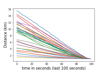
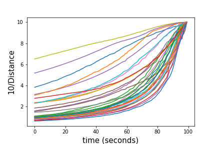
Figure 1: Distance measurements and corresponding signals extracted from datasets on aircraft trajectories collected from aircraft around the Pittsburgh-Butler Regional Airport [12].

The problem of quickest change detection with non-stationary post-change distribution is encountered in the following applications:

1. Satellite safety: As discussed in [4], one of the major challenges in satellite safety is to detect approaching debris that can cause damage to the satellite. As debris approaches the satellite, the corresponding measurements are expected to grow stochastically with time leading to a non-stationary post-change process.

2. Military applications: A classical problem in military applications is the problem of detection of an arriving enemy aircraft or an enemy object [4]. Similar to the satellite safety example, an approaching aircraft will lead to a stochastically growing process. As an example, in Fig. 1, we have plotted distance and signal measurements extracted from aircraft trajectory datasets collected around Pittsburgh-Butler Regional Airport [12].

3. Public health application: In the post-COVID-19 pandemic era, it is of significant interest to detect the onset of a pandemic. In Fig. 2, we have plotted the daily infection numbers for Allegheny and St. Louis counties for the first $200$ days starting $2020/1/22$. As seen in the figure, the numbers grow and then subside over time.

4. Social networking: Another possible application is trend detection in social network data. The trending topic will cause a sudden increase in the number of messages, and these numbers can fluctuate over time.

In all the above applications, the exact manner in which the change will occur is generally not known to the decision-maker, and they may have to take a conservative approach to the design of the detection system. A robust solution can guarantee that all possible post-change scenarios can be detected.

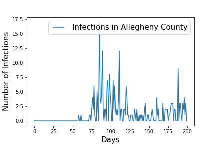
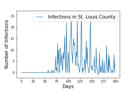
Figure 2: Daily infection rates for Allegheny and St. Louis counties in the first $200$ days starting 2020/1/22. The number of infections over time (even beyond the dates shown here) has multiple cycles of high values and low values.

2 Model and Bayesian Problem Formulation

Our change point model is as specified in (8). Specifically, we assume that we observe a sequence of independent random variables $\{X_{n}\}$ over time. Before a point $\nu$, called a change point in the following, the process is i.i.d. with density $f$. After time $\nu$, the law of the process changes to a sequence of densities $\{g_{n,\nu}\}$. Mathematically,

$$X_{n}\sim\begin{cases}f,&\quad\forall n<\nu,\\ g_{n,\nu}&\quad\forall n\geq\nu.\end{cases}$$ (9)

Thus, the post-change distribution may depend on the change point $\nu$. The post-change densities are assumed to satisfy

$$D(g_{n,\nu}\;\|\;f)>0,\quad\text{for all }n\geq 1,\;\nu\geq 1,\;n\geq\nu,$$ (10)

where $D(g\;\|\;f)=\int g(x)\log[g(x)/f(x)]dx$ is the Kullback-Leibler divergence between densities $g$ and $f$. As mentioned in the introduction, with a slight abuse of notation (borrowing it from the time-series literature [16]), we will refer to a process with densities $\{g_{n,\nu}\}$ as a non-stationary process since the density of the data evolves or changes with time. Below, we use the notation $G=\{g_{n,\nu}\}$ to denote the post-change sequence of densities.

For the problem of robust quickest change detection in non-stationary processes, we assume that the post-change law $G$ is unknown. However, there are families of distributions $\{\mathcal{P}_{n,\nu}\}$ such that

$$g_{n,\nu}\in\mathcal{P}_{n,\nu},\quad n,\nu=1,2,\dots,$$

and the families $\{\mathcal{P}_{n,\nu}\}$ are known to the decision maker.

Let $\tau$ be a stopping time for the process $\{X_{n}\}$, i.e., a positive integer-valued random variable such that the event $\{\tau\leq n\}$ belongs to the $\sigma$-algebra generated by $X_{1},\cdots,X_{n}$. In other words, whether or not $\tau\leq n$ is completely determined by the first $n$ observations. We declare that a change has occurred at the stopping time $\tau$. To find the best stopping time to detect the change in distribution, we need a performance criterion. Towards this end, we model the change point $\nu$ as a random variable with a prior distribution given by

$$\pi_{n}=\mathsf{P}(\nu=n),\quad\text{ for }n=1,2,\cdots.$$

For each $n\in\mathbb{N}$, we use $\mathsf{P}_{n}^{G}$ to denote the law of the observation process $\{X_{n}\}$ when the change occurs at $\nu=n$ and the post-change law is given by $G$. We use $\mathsf{E}_{n}^{G}$ to denote the corresponding expectation. The notations $\mathsf{P}_{\infty}^{G}=\mathsf{P}_{\infty}$ and $\mathsf{E}_{\infty}^{G}=\mathsf{E}_{\infty}$ are used when the change occurs at $n=\infty$, i.e., there is no change. Note that in case of no change, the superscript $G$ can be dropped from the notation as the post-change law plays no role. Using this notation, we define the average probability measure

$$\mathsf{P}^{\pi,G}=\sum_{n=1}^{\infty}\pi_{n}\;\mathsf{P}_{n}^{G}.$$

To capture a penalty for the false alarms, in the event that the stopping time occurs before the change, we use the probability of a false alarm defined as

$$\mathsf{P}^{\pi,G}(\tau<\nu).$$

Note that the probability of a false alarm $\mathsf{P}^{\pi,G}(\tau<\nu)$ is not a function of the post-change law $G$. This is because

$$\mathsf{P}^{\pi,G}(\tau<\nu)=\sum_{n=1}^{\infty}\pi_{n}\mathsf{P}_{n}^{G}(\tau<n)=\sum_{n=1}^{\infty}\pi_{n}\mathsf{P}_{\infty}(\tau<n),$$

where the last equality follows because $\{\tau<n\}$ is a function of $X_{1},\dots,X_{n-1}$, and the law of $X_{1},\dots,X_{n-1}$ is the same under both $\mathsf{P}_{n}^{G}$ and $\mathsf{P}_{\infty}$. Hence, in the following, we suppress the mention of $G$ and refer to the probability of false alarm only by

$$\mathsf{P}^{\pi}(\tau<\nu).$$

To penalize the detection delay, we use the average detection delay given by

$$\mathsf{E}^{\pi,G}\left[(\tau-\nu)^{+}\right],$$

where $x^{+}=\max\{x,0\}$. The optimization problem we are interested in solving is

$$\inf_{\tau\in\mathbf{C}_{\alpha}}\;\;\sup_{G}\;\mathsf{E}^{\pi,G}\left[(\tau-\nu)^{+}\right],$$ (11)

where

$$\mathbf{C}_{\alpha}=\left\{\tau:\mathsf{P}^{\pi}(\tau<\nu)\leq\alpha\right\},$$

and $\alpha$ is a given constraint on the probability of a false alarm.

2.1 Robust Optimal Algorithm in a Bayesian Setting

We now assume that the post-change law $G$ is unknown and provide the optimal or asymptotically optimal solution to (11) under assumptions on the families of post-change uncertainty classes $\{\mathcal{P}_{n,\nu}\}$. Specifically, we extend the results in [20] for i.i.d. processes and those in [10] for independent and periodically identically distributed (i.p.i.d.) processes to non-stationary processes. We assume in the rest of this section that all densities involved are equivalent to each other (absolutely continuous with respect to each other). Also, we assume in this section that the change point $\nu$ is a geometrically distributed random variable. The non-Bayesian and minimax setting is studied in Section 3.

To state the assumptions on $\{\mathcal{P}_{n,\nu}\}$, we need some definitions. We say that a random variable $Z_{2}$ is stochastically larger than another random variable $Z_{1}$ if

$$\mathsf{P}(Z_{2}\geq t)\geq\mathsf{P}(Z_{1}\geq t),\quad\text{for all }t\in\mathbb{R}.$$

We use the notation

$$Z_{2}\succ Z_{1}.$$

If $\mathcal{L}_{Z_{2}}$ and $\mathcal{L}_{Z_{1}}$ are the probability laws of $Z_{2}$ and $Z_{1}$, then we also use the notation

$$\mathcal{L}_{Z_{2}}\succ\mathcal{L}_{Z_{1}}.$$

We now introduce the notion of stochastic boundedness in non-stationary processes. In the following, we use

$$\mathcal{L}(\phi(X),g)$$

to denote the law of some function $\phi(X)$ of the random variable $X$, when the variable $X$ has density $g$.

Definition 2.1 (Stochastic Boundedness in Non-Stationary Processes; Least Favorable Law (LFL)).

We say that the family $\{\mathcal{P}_{n,\nu}\}$ is stochastically bounded by the sequence

$$\bar{G}=\{\bar{g}_{n,\nu}\},$$

and call $\bar{G}$ the least favorable law (LFL), if

$$\bar{g}_{n,\nu}\in\mathcal{P}_{n,\nu},\quad n=1,2,\dots,$$

and

$$\begin{split}\mathcal{L}\left(\log\frac{\bar{g}_{n,\nu}(X_{n})}{f(X_{n})},g_{n,\nu}\right)&\succ\mathcal{L}\left(\log\frac{\bar{g}_{n,\nu}(X_{n})}{f(X_{n})},\bar{g}_{n,\nu}\right),\quad\text{for all }\;g_{n,\nu}\in\mathcal{P}_{n,\nu},\quad n,\nu=1,2,\dots.\end{split}$$ (12)

Let

$$R_{n}=\frac{1}{(1-\rho)^{n}}\sum_{k=1}^{n}(1-\rho)^{k-1}\rho\;\prod_{i=k}^{n}\frac{\bar{g}_{i,k}(X_{i})}{f(X_{i})}$$

be the Shiryaev statistic for the LFL $\bar{G}$. Also let $\bar{\tau}^{*}$ be the stopping rule

$$\bar{\tau}^{*}=\inf\{n\geq 1:R_{n}\geq A_{n,\alpha}\}.$$ (13)

Here thresholds $A_{n,\alpha}$ are chosen to satisfy the constraint on the probability of false alarm. We note that additional assumptions are needed on the densities $\{\bar{g}_{n,\nu}\}$ to guarantee optimality or asymptotic optimality of the Shiryaev stopping rule (13). For some general conditions, see [18, 17, 19, 2].

We now state our main result on robust Bayesian quickest change detection in non-stationary processes.

Theorem 2.2.

Suppose the following conditions hold:

1. The family $\{\mathcal{P}_{n,\nu}\}$ is stochastically bounded by the law

   $$\bar{G}=\{\bar{g}_{n,\nu}\}.$$

   Thus, $\bar{G}=\{\bar{g}_{n,\nu}\}$ is the LFL.

2. Let $\alpha\in(0,1)$ be a constraint such that

   $$\mathsf{P}^{\pi}(\bar{\tau}^{*}<\nu)=\alpha,$$

   where $\bar{\tau}^{*}$ is the optimal rule designed using the LFL (13).

3. All likelihood ratio functions involved are continuous.

4. The change point $\nu$ is geometrically distributed.

5. The Shiryaev statistic (13) is optimal (respectively, asymptotically optimal) for the LFL.

Then, the stopping rule $\bar{\tau}^{*}$ in (13) designed using the LFL is optimal (respectively, asymptotically optimal) for the robust constraint problem in (11).

Proof.

The key step in the proof is to show that for each $k\in\mathbb{N}$,

$$\begin{split}\mathsf{E}_{k}^{\bar{G}}&\left[(\bar{\tau}^{*}-k)^{+}|\mathcal{F}_{k-1}\right]\geq\mathsf{E}_{k}^{G}\left[(\bar{\tau}^{*}-k)^{+}|\mathcal{F}_{k-1}\right]\quad\text{ for all }G,\end{split}$$ (14)

where $\mathcal{F}_{k-1}$ is the $\sigma$-algebra generated by $X_{1},\dots,X_{k-1}$. If the above statement is true, then by taking expectation and then taking an average over the prior on the change point, we get

$$\begin{split}\mathsf{E}^{\pi,\bar{G}}\left[(\bar{\tau}^{*}-\nu)^{+}\right]&=\sum_{k}\pi_{k}\mathsf{E}_{k}^{\bar{G}}\left[(\bar{\tau}^{*}-k)^{+}\right]\\ &\geq\sum_{k}\pi_{k}\mathsf{E}_{k}^{G}\left[(\bar{\tau}^{*}-k)^{+}\right]=\mathsf{E}^{\pi,G}\left[(\bar{\tau}^{*}-\nu)^{+}\right],\text{ for all }G.\end{split}$$ (15)

The last equation gives

$$\begin{split}\mathsf{E}^{\pi,\bar{G}}&\left[(\bar{\tau}^{*}-\nu)^{+}\right]\geq\mathsf{E}^{\pi,G}\left[(\bar{\tau}^{*}-\nu)^{+}\right],\text{ for all }G.\end{split}$$ (16)

This implies that

$$\begin{split}\mathsf{E}^{\pi,\bar{G}}&\left[(\bar{\tau}^{*}-\nu)^{+}\right]=\sup_{G}\mathsf{E}^{\pi,G}\left[(\bar{\tau}^{*}-\nu)^{+}\right],\end{split}$$ (17)

where we have equality because the law $\bar{G}$ belongs to the family considered on the right. Now, if $\tau$ is any stopping rule satisfying the probability of false alarm constraint of $\alpha$, then since $\bar{\tau}^{*}$ is the optimal test for the LFL $\bar{G}$, we have

$$\begin{split}\sup_{G}\mathsf{E}^{\pi,G}\left[(\tau-\nu)^{+}\right]&\geq\mathsf{E}^{\pi,\bar{G}}\left[(\tau-\nu)^{+}\right]\geq\mathsf{E}^{\pi,\bar{G}}\left[(\bar{\tau}^{*}-\nu)^{+}\right](1+o(1))\\ &=\sup_{G}\mathsf{E}^{\pi,G}\left[(\bar{\tau}^{*}-\nu)^{+}\right](1+o(1)).\end{split}$$ (18)

The last equation proves the robust optimality of the stopping rule $\bar{\tau}^{*}$ for the problem in (11). We note that if the rule $\bar{\tau}^{*}$ is exactly optimal for $\bar{G}$, then the $o(1)$ terms will be identically zero, and we will get exact robust optimality of $\bar{\tau}^{*}$ for the post-change family.

We now prove the key step (14). Towards this end, we prove that for every integer $N\geq 0$,

$$\begin{split}\mathsf{P}_{k}^{\bar{G}}\left[(\bar{\tau}^{*}-k)^{+}>N|\mathcal{F}_{k-1}\right]&\geq\mathsf{P}_{k}^{G}\left[(\bar{\tau}^{*}-k)^{+}>N|\mathcal{F}_{k-1}\right],\text{ for all }G.\end{split}$$ (19)

Equation (19) implies (14) because through (19) we would establish that $(\bar{\tau}^{*}-k)^{+}$ is stochastically bigger under the conditional distribution when the law is $\bar{G}$ and the conditioning is on $\mathcal{F}_{k-1}$. In fact, a summation over $N$ in (19) would imply (14).

Equation (19) is trivially true for $N=0$ since event $\{(\bar{\tau}^{*}-k)^{+}>0\}$ is $\mathcal{F}_{k-1}$-measurable. So we only prove it for $N\geq 1$. Towards this end, we first have

$$\begin{split}\mathsf{P}_{k}^{\bar{G}}\left[(\bar{\tau}^{*}-k)^{+}\leq N|\mathcal{F}_{k-1}\right]&=\mathsf{P}_{k}^{\bar{G}}\left[\bar{\tau}^{*}\leq k+N|\mathcal{F}_{k-1}\right]\\ &=\mathsf{P}_{k}^{\bar{G}}\left[f(X_{1},X_{2},\dots,X_{k+N})\;\geq\;0\;|\;\mathcal{F}_{k-1}\right],\end{split}$$ (20)

where the function $f(z_{1},z_{2},\dots,z_{N})$ is given by

$$\begin{split}f&(z_{1},z_{2},\dots,z_{N})\\ &=\max_{1\leq n\leq N}\left(\frac{1}{(1-\rho)^{n}}\sum_{k=1}^{n}(1-\rho)^{k-1}\rho\;\exp\left(\sum_{i=k}^{n}\log[\bar{g}_{i,k}(z_{i})/f(z_{i})]\right)-A_{n,\alpha}\right).\end{split}$$ (21)

Using the stochastic boundedness assumption,

$$\begin{split}\mathcal{L}\left(\log\frac{\bar{g}_{n,\nu}(X_{n})}{f(X_{n})},g_{n,\nu}\right)&\succ\mathcal{L}\left(\log\frac{\bar{g}_{n,\nu}(X_{n})}{f(X_{n})},\bar{g}_{n,\nu}\right),\quad\text{for all }\;g_{n,\nu}\in\mathcal{P}_{n,\nu},\quad n,\nu=1,2,\dots,\end{split}$$

and the fact that $f(z_{1},z_{2},\dots,z_{N})$ is continuous and increasing in $\log[\bar{g}_{i,k}(z_{i})/f(z_{i})]$, we have by Lemma III.1 in [20] that

$$\begin{split}\mathsf{P}_{k}^{\bar{G}}\left[(\bar{\tau}^{*}-k)^{+}\leq N\;|\;\mathcal{F}_{k-1}\right]&=\mathsf{P}_{k}^{\bar{G}}\left[\bar{\tau}^{*}\leq k+N\;|\;\mathcal{F}_{k-1}\right]\\ &=\mathsf{P}_{k}^{\bar{G}}\left[f(X_{1},X_{2},\dots,X_{k+N})\geq 0\;|\;\mathcal{F}_{k-1}\right]\\ &\leq\mathsf{P}_{k}^{{G}}\left[f(X_{1},X_{2},\dots,X_{k+N})\geq 0\;|\;\mathcal{F}_{k-1}\right]\\ &=\mathsf{P}_{k}^{G}\left[\bar{\tau}^{*}\leq k+N\;|\;\mathcal{F}_{k-1}\right]\\ &=\mathsf{P}_{k}^{{G}}\left[(\bar{\tau}^{*}-k)^{+}\leq N\;|\;\mathcal{F}_{k-1}\right],\quad\text{ for all }G.\end{split}$$ (22)

This proves (19) and hence (14). ∎

We discuss special cases of this result and examples in Section 4, Section 5, and Section 6.

3 Minimax Problem Formulation

In this section, we obtain a solution for a robust version of the minimax problem of Lorden [8]. We have the same change point model as in Section 2. But, here we assume that the change point $\nu$ is an unknown constant and solve the following problem:

$$\inf_{\tau\in\mathbf{D}_{\alpha}}\;\;\sup_{G}\;\;\sup_{\nu}\;\operatorname*{ess\,sup}\;\mathsf{E}_{\nu}^{G}\left[(\tau-\nu+1)^{+}|\mathcal{F}_{\nu-1}\right]:=\inf_{\tau\in\mathbf{D}_{\alpha}}\;\;\sup_{G}\;\;\text{WADD}^{G}(\tau),$$ (23)

where

$$\mathbf{D}_{\alpha}=\left\{\tau:\mathsf{E}_{\infty}[\tau]=\frac{1}{\alpha}\right\}.$$

Let

$$W_{n}=\max_{1\leq k\leq n}\sum_{i=k}^{n}\frac{\bar{g}_{i,k}(X_{i})}{f(X_{i})}$$

be the generalized CUSUM statistic for the LFL $\bar{G}$. Also let $\bar{\tau}^{*}$ be the stopping rule

$$\bar{\tau_{c}}^{*}=\inf\{n\geq 1:W_{n}\geq B_{n,\alpha}\}.$$ (24)

Here thresholds $B_{n,\alpha}$ are chosen to satisfy the constraint on the mean time to a false alarm. We again note that additional assumptions are needed on the densities $\{\bar{g}_{n,\nu}\}$ to guarantee optimality or asymptotic optimality of the generalized CUSUM stopping rule (13). For some general conditions, see [6, 17, 19, 7].

We now state our main result on robust minimax quickest change detection in non-stationary processes.

Theorem 3.1.

Suppose the following conditions hold:

1. The family $\{\mathcal{P}_{n,\nu}\}$ is stochastically bounded by the law

   $$\bar{G}=\{\bar{g}_{n,\nu}\}.$$

   Thus, $\bar{G}=\{\bar{g}_{n,\nu}\}$ is the LFL.

2. Let $\alpha\in(0,1)$ be a constraint such that

   $$\mathsf{E}_{\infty}[\bar{\tau}_{c}^{*}]=\frac{1}{\alpha},$$

   where $\bar{\tau}_{c}^{*}$ is the optimal rule designed using the LFL (24).

3. All likelihood ratio functions involved are continuous.

4. The generalized CUSUM algorithm (24) is optimal (respectively, asymptotically optimal) for the LFL.

Then, the stopping rule $\bar{\tau}_{c}^{*}$ in (24) designed using the LFL is optimal (respectively, asymptotically optimal) for the robust constraint problem in (23).

Proof.

The key step in the proof is to show that for each $k\in\mathbb{N}$,

$$\begin{split}\mathsf{E}_{k}^{\bar{G}}&\left[(\bar{\tau}_{c}^{*}-k)^{+}|\mathcal{F}_{k-1}\right]\geq\mathsf{E}_{k}^{G}\left[(\bar{\tau}_{c}^{*}-k)^{+}|\mathcal{F}_{k-1}\right]\quad\text{ for all }G.\end{split}$$ (25)

This is proved in a manner similar to the previous proof. We provide the proof for completeness. Specifically, we need to show that for every integer $N\geq 0$,

$$\begin{split}\mathsf{P}_{k}^{\bar{G}}\left[(\bar{\tau}_{c}^{*}-k)^{+}>N|\mathcal{F}_{k-1}\right]&\geq\mathsf{P}_{k}^{G}\left[(\bar{\tau}_{c}^{*}-k)^{+}>N|\mathcal{F}_{k-1}\right],\text{ for all }G.\end{split}$$ (26)

This is again trivially true for $N=0$ since event $\{(\bar{\tau}^{*}-k)^{+}>0\}$ is $\mathcal{F}_{k-1}$-measurable. So we only prove it for $N\geq 1$. Towards this end, we first have

$$\begin{split}\mathsf{P}_{k}^{\bar{G}}\left[(\bar{\tau}_{c}^{*}-k)^{+}\leq N|\mathcal{F}_{k-1}\right]&=\mathsf{P}_{k}^{\bar{G}}\left[\bar{\tau}_{c}^{*}\leq k+N|\mathcal{F}_{k-1}\right]\\ &=\mathsf{P}_{k}^{\bar{G}}\left[h(X_{1},X_{2},\dots,X_{k+N})\;\geq\;0\;|\;\mathcal{F}_{k-1}\right],\end{split}$$ (27)

where now the function $h(z_{1},z_{2},\dots,z_{N})$ is given by

$$\begin{split}h&(z_{1},z_{2},\dots,z_{N})=\max_{1\leq n\leq N}\left(\max_{1\leq k\leq n}\left(\sum_{i=k}^{n}\log[\bar{g}_{i,k}(z_{i})/f(z_{i})]\right)-B_{n,\alpha}\right).\end{split}$$ (28)

Again, using the stochastic boundedness assumption,

$$\begin{split}\mathcal{L}\left(\log\frac{\bar{g}_{n,\nu}(X_{n})}{f(X_{n})},g_{n,\nu}\right)&\succ\mathcal{L}\left(\log\frac{\bar{g}_{n,\nu}(X_{n})}{f(X_{n})},\bar{g}_{n,\nu}\right),\quad\text{for all }\;g_{n,\nu}\in\mathcal{P}_{n,\nu},\quad n,\nu=1,2,\dots,\end{split}$$

and the fact that even $h(z_{1},z_{2},\dots,z_{N})$ is continuous and increasing in $\log[\bar{g}_{i,k}(z_{i})/f(z_{i})]$, we have by Lemma III.1 in [20] that

$$\begin{split}\mathsf{P}_{k}^{\bar{G}}\left[(\bar{\tau}_{c}^{*}-k)^{+}\leq N\;|\;\mathcal{F}_{k-1}\right]&=\mathsf{P}_{k}^{\bar{G}}\left[\bar{\tau}_{c}^{*}\leq k+N\;|\;\mathcal{F}_{k-1}\right]\\ &=\mathsf{P}_{k}^{\bar{G}}\left[h(X_{1},X_{2},\dots,X_{k+N})\geq 0\;|\;\mathcal{F}_{k-1}\right]\\ &\leq\mathsf{P}_{k}^{{G}}\left[h(X_{1},X_{2},\dots,X_{k+N})\geq 0\;|\;\mathcal{F}_{k-1}\right]\\ &=\mathsf{P}_{k}^{G}\left[\bar{\tau}_{c}^{*}\leq k+N\;|\;\mathcal{F}_{k-1}\right]\\ &=\mathsf{P}_{k}^{{G}}\left[(\bar{\tau}_{c}^{*}-k)^{+}\leq N\;|\;\mathcal{F}_{k-1}\right],\quad\text{ for all }G.\end{split}$$ (29)

This proves (26) and hence (25).

Thus, we have

$$\begin{split}\mathsf{E}_{k}^{\bar{G}}&\left[(\bar{\tau}_{c}^{*}-k)^{+}|\mathcal{F}_{k-1}\right]\geq\mathsf{E}_{k}^{G}\left[(\bar{\tau}_{c}^{*}-k)^{+}|\mathcal{F}_{k-1}\right]\quad\text{ for all }G.\end{split}$$ (30)

This implies (by the definition of essential supremum)

$$\begin{split}\operatorname*{ess\,sup}\;\mathsf{E}_{k}^{\bar{G}}&\left[(\bar{\tau}_{c}^{*}-k)^{+}|\mathcal{F}_{k-1}\right]\geq\operatorname*{ess\,sup}\;\;\mathsf{E}_{k}^{G}\left[(\bar{\tau}_{c}^{*}-k)^{+}|\mathcal{F}_{k-1}\right]\quad\text{ for all }G.\end{split}$$ (31)

Since (31) is true for every $k$, we have

$$\begin{split}\sup_{k}\;\operatorname*{ess\,sup}\;\mathsf{E}_{k}^{\bar{G}}&\left[(\bar{\tau}_{c}^{*}-k)^{+}|\mathcal{F}_{k-1}\right]\geq\sup_{k}\;\operatorname*{ess\,sup}\;\;\mathsf{E}_{k}^{G}\left[(\bar{\tau}_{c}^{*}-k)^{+}|\mathcal{F}_{k-1}\right]\quad\text{ for all }G.\end{split}$$ (32)

This gives us

$$\sup_{k}\;\operatorname*{ess\,sup}\;\mathsf{E}_{k}^{\bar{G}}\left[(\bar{\tau}_{c}^{*}-k)^{+}|\mathcal{F}_{k-1}\right]=\sup_{G}\;\sup_{k}\;\operatorname*{ess\,sup}\;\;\mathsf{E}_{k}^{G}\left[(\bar{\tau}_{c}^{*}-k)^{+}|\mathcal{F}_{k-1}\right],$$ (33)

or

$$\text{WADD}^{\bar{G}}(\bar{\tau}_{c}^{*})=\sup_{G}\text{WADD}^{{G}}(\bar{\tau}_{c}^{*}).$$ (34)

Now, if $\tau$ is any stopping rule satisfying the mean time to false alarm constraint of $\alpha$, then since $\bar{\tau}^{*}$ is the optimal test for the LFL $\bar{G}$, we have

$$\begin{split}\sup_{G}\text{WADD}^{{G}}({\tau})\geq\text{WADD}^{\bar{G}}({\tau})\geq&\text{WADD}^{\bar{G}}(\bar{\tau}_{c}^{*})(1+o(1))\\ =&\sup_{G}\text{WADD}^{{G}}(\bar{\tau}_{c}^{*})(1+o(1)).\end{split}$$ (35)

The last equation proves the robust optimality of the stopping rule $\bar{\tau}_{c}^{*}$ for the problem in (23). We again note that if the rule $\bar{\tau}_{c}^{*}$ is exactly optimal for $\bar{G}$, then the $o(1)$ terms will be identically zero, and we will get exact robust optimality of $\bar{\tau}_{c}^{*}$ for the post-change family. ∎

4 Exact Robust Optimality in Non-Stationary Processes

In this section, we discuss two special cases where the robust optimality stated in the previous section is exact.

When the LFL $\{g_{n,\nu}\}$ satisfies the special condition that

$$\bar{g}_{n,\nu}=\bar{g},\quad\forall n,\nu,$$ (36)

then the robust optimal algorithms reduce to the classical Shiryaev and CUSUM algorithm for the i.i.d. setting and hence are exactly optimal for their corresponding formulations. We note that this result is different from that studied in [20] because in [20] the post-change model is also unknown but assumed to be i.i.d., but here the post-change process is allowed to be any non-stationary process. We state this as a corollary.

Corollary 4.1.

In Theorem 2.2 and Theorem 3.1, if the LFL $\{g_{n,\nu}\}$ satisfies the special condition that

$$\bar{g}_{n,\nu}=\bar{g},\quad\forall n,\nu,$$ (37)

then the generalized Shiryaev algorithm designed using the LFL reduces to the classical Shiryaev algorithm with post-change density $\bar{g}$ with recursively implementable statistic

$$R_{n}=\frac{R_{n-1}+\rho}{1-\rho}\;\frac{\bar{g}(X_{n})}{f(X_{n})},\quad R_{0}=0,$$ (38)

and is exactly optimal for the robust problem stated in (11). For the same reasons, the generalized CUSUM algorithm designed using the LFL reduces to the classical CUSUM algorithm with recursively implementable statistic

$$W_{n}=\left(W_{n-1}+\log\frac{\bar{g}(X_{n})}{f(X_{n})}\right)^{+},\quad\quad W_{0}=0,$$ (39)

and is exactly robust optimal for the problem stated in (23).

Another case where the generalized Shiryaev test is exactly optimal is when the LFL is an independent and periodically identically distributed (i.p.i.d.) process, i.e.,

$$\bar{g}_{n,\nu}=\bar{g}_{n},$$

and the sequence $\{g_{n}\}$ is periodic:

$$\bar{g}_{n+T}=\bar{g}_{n},\quad\text{for some positive integer }T.$$

For this case, it is shown in [2] that the generalized Shiryaev algorithm is exactly optimal for a periodic sequence of thresholds: $A_{n,\alpha}=A_{n+T,\alpha}$, for every $n$. We state this result also as a corollary.

Corollary 4.2.

In Theorem 2.2, if the LFL $\{g_{n,\nu}\}$ is an i.p.i.d. process, then the generalized Shiryaev algorithm is exactly robust optimal. In this, case the statistic again has a recursive update

$$R_{n}=\frac{R_{n-1}+\rho}{1-\rho}\;\frac{\bar{g}_{n}(X_{i})}{f(X_{i})},\quad R_{0}=0,$$ (40)

The equivalent result for i.p.i.d. processes and the minimax setting is not yet available.

5 General Conditions for Robust Asymptotic Optimality

When the LFL is not a fixed density, it is not known if the generalized Shiryaev or CUSUM algorithms are exactly optimal (for a fixed false alarm rate). However, their asymptotic optimality (with the false alarm rate going to zero) has been extensively studied. One set of sufficient conditions on the asymptotic optimality of the generalized CUSUM algorithm essentially follows from the work of Lai [6]. We provide them below for completeness. For the general minimax and Bayesian theory (including theory for dependent data), we refer to [6, 18, 17, 19, 7]. Define

$$Z_{n,\nu}=\log\frac{\bar{g}_{n,\nu}(X_{n})}{f(X_{n})}$$

to be the log-likelihood ratio at time $n$ when the change occurs at $\nu$ for the LFL.

Theorem 5.1 ([6], [4]).

1. Let there exist a positive number $I$ such that the bivariate log likelihood ratios $\{Z_{n,\nu}\}$ satisfy the following condition:

   $$\begin{split}\lim_{n\to\infty}\;\sup_{\nu\geq 1}\;\operatorname*{ess\,sup}\mathsf{P}_{\nu}^{\bar{G}}&\left(\max_{t\leq n}\sum_{i=\nu}^{\nu+t}Z_{i,\nu}\geq I(1+\delta)n\;\bigg{|}\;X_{1},\dots,X_{\nu-1}\right)=0.\end{split}$$ (41)

   Then, we have the universal lower bound as $\gamma\to\infty$,

   $$\begin{split}\min_{\tau}\;\sup_{\nu\geq 1}\;&\operatorname*{ess\,sup}\;\mathsf{E}_{\nu}^{\bar{G}}[(\tau-\nu+1)^{+}|X_{1},\dots,X_{\nu-1}]\quad\geq\quad\frac{\log\gamma}{I}(1+o(1)).\end{split}$$ (42)

   Here the minimum over $\tau$ is over those stopping times satisfying $\mathsf{E}_{\infty}[\tau]\geq\gamma$.

2. The generalized CUSUM algorithm,

   $$\tau_{c}^{*}=\min\left\{n\geq 1:\max_{1\leq k\leq n}\sum_{i=k}^{n}Z_{i,k}\geq\log(\gamma)\right\},$$

   satisfies

   $$\mathsf{E}_{\infty}[\tau_{c}^{*}]\geq\gamma.$$

3. Furthermore, if the bivariate log-likelihood ratios $\{Z_{n,\nu}\}$ also satisfy

   $$\begin{split}\lim_{n\to\infty}\;\sup_{k\geq\nu\geq 1}\;\operatorname*{ess\,sup}\mathsf{P}_{\nu}^{\bar{G}}&\left(\frac{1}{n}\sum_{i=k}^{k+n}Z_{i,k}\leq I-\delta\;\bigg{|}\;X_{1},\dots,X_{k-1}\right)=0.\end{split}$$ (43)

   Then as $\gamma\to\infty$, $\tau_{c}^{*}$ achieves the lower bound:

   $$\begin{split}\sup_{\nu\geq 1}\;\operatorname*{ess\,sup}\;\mathsf{E}_{\nu}^{\bar{G}}&[(\tau_{c}^{*}-\nu+1)^{+}|X_{1},\dots,X_{\nu-1}]\leq\frac{\log\gamma}{I}(1+o(1)),\quad\gamma\to\infty.\end{split}$$ (44)

This theorem establishes the fact that if the conditions in the above theorem are satisfied, then the generalized CUSUM algorithm is minimax asymptotically robust and optimal for the problem in (23). A similar result can also be stated for the generalized Shiryaev algorithm [18, 17, 19]. When we have

$$\bar{g}_{n,\nu}=\bar{g},\quad\forall n,\nu,$$ (45)

the above theorem provides a performance analysis of the robust CUSUM algorithm. In this case, it can be shown that $I=D(\bar{g}\;\|\;f)$, choosing threshold $A=\log\gamma$ ensures

$$\mathsf{E}_{\infty}[\tau_{c}^{*}]\geq\gamma.$$ (46)

In addition, as $A=\log\gamma\to\infty$, we have

$$\mathsf{E}_{1}[\tau_{c}^{*}]=\frac{\log(\gamma)}{D(\bar{g}\;\|\;f)}(1+o(1)).$$ (47)

We now give two examples of a non-stationary process for which the above conditions are satisfied.

Example 5.2 (I.P.I.D. Process).

Recall that an i.p.i.d. process is defined as follows. A sequence $\{X_{n}\}$ is called an i.p.i.d. process if it is a sequence of independent random variables such that

$$\begin{split}X_{n}&\sim f\quad n<\nu,\\ &\sim g_{n}\quad n\geq\nu,\end{split}$$ (48)

and that there exists a positive integer $T$ such that

$$g_{n+T}=g_{n},\quad\forall n.$$

The general asymptotic optimality theory for i.p.i.d. processes in the minimax setting is studied in [1] and it is shown there that an i.p.i.d. process satisfies the conditions of Theorem 5.1. Thus, when the densities $\{g_{n}\}$ are unknown but known to belong to a sequence of families $\mathcal{P}_{n}$:

$$g_{n}\in\mathcal{P}_{n},\quad n=1,2,\dots,T,$$

and if $\bar{g}_{n}$ is the LFL for $\mathcal{P}_{n}$ based on the definition of stochastic boundedness given above, then the generalized CUSUM algorithm designed using densities $f$ and $\bar{g}_{n}$ are robust asymptotically optimal.

Example 5.3 (MLR Order Processes).

In [4], it has been shown that the sufficient conditions of Theorem 5.1 are satisfied by a monotone likelihood ratio (MLR) order process (referred to as an exploding process in [4]). Let $\{X_{n}\}$ be a sequence of independent random variables such that

$$\begin{split}X_{n}&\sim f\quad n<\nu,\\ &\sim g_{n-\nu}\quad n\geq\nu,\end{split}$$ (49)

where $\{g_{n}\}$ is a sequence of densities increasing in MLR order:

$$\frac{g_{n+1}(x)}{g_{n}(x)}\quad\uparrow\quad x.$$

Thus, according to the results in [4] the generalized CUSUM algorithm is asymptotically optimal when the densities $\{g_{n}\}$ are known. If these densities are unknown and

$$g_{n}\in\mathcal{P}_{n},\quad\forall n,$$

and if $\{\bar{g}_{n}\}$ is the sequence of LFLs, then the generalized CUSUM algorithm designed using the LFLs is asymptotically minimax robust optimal for MLR-order processes.

6 Examples of Least Favorable Laws

In this section, we provide examples of LFL from Gaussian and Poisson families. We use the following simple lemma in these examples. Its proof can be found, for example, in [5]. We provide the proof for completeness.

Lemma 6.1.

Let $f$ and $g$ be two probability density functions such that $f$ dominated $g$ in monotone likelihood ratio (MLR) order:

$$\frac{f(x)}{g(x)}\;\;\uparrow\;\;x.$$

Then, $f$ also dominates $g$ in stochastic order, i.e.,

$$\int_{x}^{\infty}f(y)dy\geq\int_{x}^{\infty}g(y)dy,\quad\forall x.$$

Proof.

Define, $t=\sup\left\{x:\frac{f(x)}{g(x)}\leq 1\right\}$. Then, when $x\leq t$,

$$\int_{-\infty}^{x}f(y)dy\leq\int_{-\infty}^{x}g(y)dy,$$

implying $\int_{x}^{\infty}f(y)dy\geq\int_{x}^{\infty}g(y)dy.$ On the other hand, if $x>t$, then

$$\int_{x}^{\infty}f(y)dy=\int_{x}^{\infty}\frac{f(y)}{g(y)}g(y)dy\geq\int_{x}^{\infty}g(y)dy.$$

This proves the lemma. ∎

Note that the statement is valid even if the densities are with respect to a measure more general than the Lebesgue measure, including the counting measure. The latter implies that the MLR order for mass functions implies their stochastic order (this can be proved by replacing integrals with summations in the above proof).

We now give two examples of MLR order densities. By the above lemma, they are also ordered by stochastic order. First, consider two Gaussian densities $g=\mathcal{N}(\mu_{1},\sigma^{2})$ and $f=\mathcal{N}(\mu_{2},\sigma^{2})$, with $\mu_{2}>\mu_{1}$. Then since

$$\frac{f(x)}{g(x)}=\exp\left(\frac{\mu_{2}-\mu_{1}}{\sigma^{2}}x+\frac{\mu_{1}^{2}-\mu_{2}^{2}}{2\sigma^{2}}\right),$$

the ratio increases with $x$ because $(\mu_{2}-\mu_{1})\geq 0$. Next, consider two Poisson mass functions $g=\text{Pois}(\lambda_{1})$ and $f=\text{Pois}(\lambda_{2})$, with $\lambda_{2}>\lambda_{1}$. Then since

$$\frac{f(k)}{g(k)}=\left(\frac{\lambda_{2}}{\lambda_{1}}\right)^{k}e^{-\lambda_{2}+\lambda_{1}},$$

the ratio increases with $k$ because $\frac{\lambda_{2}}{\lambda_{1}}\geq 1$.

We now give two examples of non-stationary processes with specified uncertainty classes. We then identify their LFLs.

Example 6.2 (Gaussian LFL).

Let the pre-change density be given by $f=\mathcal{N}(0,1)$ and the post-change densities are given by

$$g_{n,\nu}=\mathcal{N}(\mu_{n,\nu},1).$$

Now, let for each $\nu$, $\mu_{n,\nu}$ is increasing in $n$. The means $\{\mu_{n,\nu}\}$ are not known but are believed to satisfy for some known $\{\bar{\mu}_{n,\nu}\}$,

$$\mu_{n,\nu}\geq\bar{\mu}_{n,\nu}>0,\quad\forall n,\nu,$$

Then,

$$\log\frac{\bar{g}_{n,\nu}(X)}{f(X)}=\left(\bar{\mu}_{n,\nu}\;X-\frac{\bar{\mu}_{n,\nu}^{2}}{2}\right),$$

and

$$X\sim\mathcal{N}(\bar{\mu}_{n,\nu},1) \implies\log\frac{\bar{g}_{n,\nu}(X)}{f(X)}\sim\mathcal{N}\left(\frac{\bar{\mu}_{n,\nu}^{2}}{2},\;\bar{\mu}_{n,\nu}^{2}\right)$$

$$X\sim\mathcal{N}({\mu}_{n,\nu},1) \implies\log\frac{\bar{g}_{n,\nu}(X)}{f(X)}\sim\mathcal{N}\left(\bar{\mu}_{n,\nu}\;{\mu}_{n,\nu}-\frac{\bar{\mu}_{n,\nu}^{2}}{2},\;\bar{\mu}_{n,\nu}^{2}\right).$$

Since $\mu_{n,\nu}\geq\bar{\mu}_{n,\nu}$, we have

$$\bar{\mu}_{n,\nu}\;{\mu}_{n,\nu}-\frac{\bar{\mu}_{n,\nu}^{2}}{2}\;\;\geq\;\;\frac{\bar{\mu}_{n,\nu}^{2}}{2}.$$

Thus, $\mathcal{N}\left(\bar{\mu}_{n,\nu}\;{\mu}_{n,\nu}-\frac{\bar{\mu}_{n,\nu}^{2}}{2},\;\bar{\mu}_{n,\nu}^{2}\right)$ dominates $\mathcal{N}\left(\frac{\bar{\mu}_{n,\nu}^{2}}{2},\;\bar{\mu}_{n,\nu}^{2}\right)$ in MLR order (based on the discussion after Lemma 6.1) and hence in stochastic order (by Lemma 6.1). This shows that the post-change law made with the sequence of densities $\{\mathcal{N}(\bar{\mu}_{n,\nu},1)\}$ is the LFL.

We now give an example of LFL from the Poisson family of distributions.

Example 6.3 (Poisson LFL).

Let the pre-change density be given by $f=\text{Pois}(\lambda_{0})$ and the post-change densities are given by

$$g_{n,\nu}=\text{Pois}(\lambda_{n,\nu}).$$

Now, let for each $\nu$, $\lambda_{n,\nu}$ is increasing in $n$. The means $\{\lambda_{n,\nu}\}$ are not known but are believed to satisfy for some known $\{\bar{\lambda}_{n,\nu}\}$,

$$\lambda_{n,\nu}\geq\bar{\lambda}_{n,\nu}>\lambda_{0},\quad\forall n,\nu,$$

Then,

$$\log\frac{\bar{g}_{n,\nu}(X)}{f(X)}=\log\left[\left(\frac{\bar{\lambda}_{n,\nu}}{\lambda_{0}}\right)^{X}e^{-\bar{\lambda}_{n,\nu}+\lambda_{0}}\right]=X\log\left(\frac{\bar{\lambda}_{n,\nu}}{\lambda_{0}}\right)-\bar{\lambda}_{n,\nu}+\lambda_{0},$$

and

$$X\sim\text{Pois}(\bar{\lambda}_{n,\nu}) \implies\log\frac{\bar{g}_{n,\nu}(X)}{f(X)}\sim\text{Pois}\left(\bar{\lambda}_{n,\nu}\log\left(\frac{\bar{\lambda}_{n,\nu}}{\lambda_{0}}\right)-\bar{\lambda}_{n,\nu}+\lambda_{0}\right)$$

$$X\sim\text{Pois}({\lambda}_{n,\nu}) \implies\log\frac{\bar{g}_{n,\nu}(X)}{f(X)}\sim\text{Pois}\left({\lambda}_{n,\nu}\log\left(\frac{\bar{\lambda}_{n,\nu}}{\lambda_{0}}\right)-\bar{\lambda}_{n,\nu}+\lambda_{0}\right).$$

We note that while the support of the random variable $\log\frac{\bar{g}_{n,\nu}(X)}{f(X)}$ is

$$\left\{k\log\left(\frac{\bar{\lambda}_{n,\nu}}{\lambda_{0}}\right)-\bar{\lambda}_{n,\nu}+\lambda_{0}\right\},\quad k=0,1,2,3,\dots,$$

its law is completely characterized by a Poisson distribution. This is what we represent using the $\sim$ sign above. Since $\lambda_{n,\nu}\geq\bar{\lambda}_{n,\nu}$, we have

$$\left({\lambda}_{n,\nu}\log\left(\frac{\bar{\lambda}_{n,\nu}}{\lambda_{0}}\right)-\bar{\lambda}_{n,\nu}+\lambda_{0}\right)\geq\left(\bar{\lambda}_{n,\nu}\log\left(\frac{\bar{\lambda}_{n,\nu}}{\lambda_{0}}\right)-\bar{\lambda}_{n,\nu}+\lambda_{0}\right).$$

Thus, $\text{Pois}\left({\lambda}_{n,\nu}\log\left(\frac{\bar{\lambda}_{n,\nu}}{\lambda_{0}}\right)-\bar{\lambda}_{n,\nu}+\lambda_{0}\right)$ dominates $\text{Pois}\left(\bar{\lambda}_{n,\nu}\log\left(\frac{\bar{\lambda}_{n,\nu}}{\lambda_{0}}\right)-\bar{\lambda}_{n,\nu}+\lambda_{0}\right)$ in MLR order (based on the discussion after Lemma 6.1) and hence in stochastic order (by Lemma 6.1). This shows that the post-change law made with the sequence of densities $\{\text{Pois}(\bar{\lambda}_{n,\nu})\}$ is the LFL.

7 Numerical Results

In this section, we show the effectiveness of the robust tests on real and simulated data.

7.1 Application to Simulated Gaussian and Poisson Data

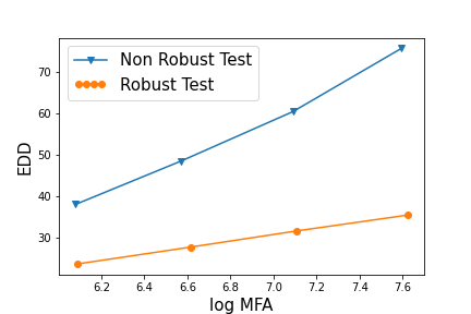
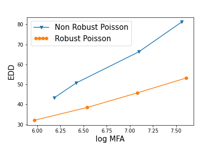
Figure 3: [Left] Comparison of robust CUSUM algorithm designed using pre-change density $f=\mathcal{N}(0,1)$ and post-change density $\mathcal{N}(0.5,1)$ with a non-robust test designed using pre-change density $f=\mathcal{N}(0,1)$ and post-change density $\mathcal{N}(1.5,1)$. The data samples are generated after change using $\mathcal{N}(0.5,1)$. [Right] A similar plot for Poisson laws, with $f=\text{Pois}(0.5)$, LFL as $\text{Pois}(0.8)$, non-robust post-change as $\text{Pois}(1.5)$, and data samples are generated from $\text{Pois}(0.8)$. Here EDD is used to denote $\mathsf{E}_{1}^{\bar{G}}[\tau_{c}^{*}-1]$.

For the Gaussian case, we choose the following model:

$$\begin{split}f=\mathcal{N}(0,1),\quad\quad g_{n,\nu}=\mathcal{N}(\mu_{n,\nu},1),\quad\quad\mu_{n,\nu}\geq 0.5.\end{split}$$ (50)

From Example 6.2, it follows that the LFL is $\mathcal{N}(0.5,1)$. Thus, the CUSUM and Shiryaev test designed with pre-change density $f=\mathcal{N}(0,1)$ and post-change density $\mathcal{N}(0.5,1)$ are robust optimal. In Fig. 3 (Left), we have compared the robust CUSUM test with a randomly picked non-robust test designed using pre-change density $f=\mathcal{N}(0,1)$ and post-change density $\mathcal{N}(1.5,1)$. The data samples after change for the simulations are generated using $\mathcal{N}(0.5,1)$. This data generation corresponds to the worst-case scenario, and as expected, the worst-case performance of the robust test is better than that of a non-robust test.

For the Poisson case, we chose the following model:

$$\begin{split}f=\text{Pois}(0.5),\quad\quad g_{n,\nu}=\text{Pois}(\lambda_{n,\nu}),\quad\quad\lambda_{n,\nu}\geq 0.8.\end{split}$$ (51)

Thus, following Example 6.3, the LFL is $\text{Pois}(0.5)$. We compare it with a randomly chosen non-robust test with post-change law $\text{Pois}(1.5)$. The data for the Poisson case was generated using the worst-case scenario $\text{Pois}(0.8)$; See Fig. 3 (Right).

In Fig. 4, we have shown the corresponding comparisons for the robust Shiryaev test using the same Gaussian and Poisson models as above. The change point is assumed to be a geometric random variable with parameter $0.01$.

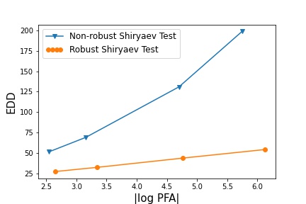
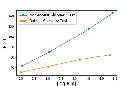
Figure 4: Comparisons for the robust Shiryaev test. These two figures were generated using the same setup used for generating Fig. 3. In addition, the change point is assumed to be a geometric random variable with parameter $0.01$. Here EDD represents $\mathsf{E}[(\tau^{*}-\nu)^{+}]$.

7.2 Applying Robust CUSUM Test to Pittsburgh Flight Data

In this section, we apply the robust CUSUM test to detect the arrival of aircraft based on data collected around Pittsburgh-Butler Regional Airport [12]. The distance measurements for the last $100$ seconds for randomly selected $35$ flights are shown in Fig. 1. We converted these distance measurements to signals by using the transformation $\frac{10}{\text{Distance}}$ (again see Fig. 1). We then added $\mathcal{N}(0,1)$ noise after padding $100$ zeros at the beginning of the signals (see Fig. 5). The noise is also added to simulate a scenario where an approaching enemy is being detected in a noisy environment.

Inspired by Example 6.2, we design a robust CUSUM algorithm by selecting the pre-change density as $\mathcal{N}(0,1)$ and the post-change as $\mathcal{N}(0.64,1)$. Here $0.64$ is the minimum value of the flight signal across all $35$ flights. We choose the threshold $6.9=\log(1000)$ to ensure that the mean time to a false alarm (MFA) is greater than $1000$; see (46). The robust CUSUM statistics for all $35$ aircraft are plotted in Fig. 6 (Left) with the delay profile plotted on the right. The average detection delay over the delay paths was found to be $10.8$ seconds.

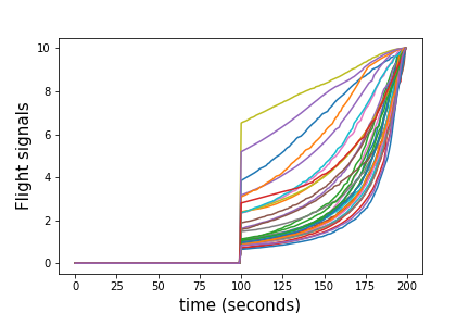
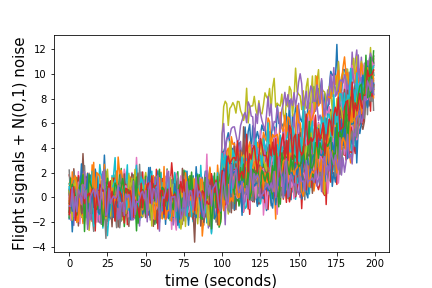
Figure 5: [Left] Flight signals for the last $100$ seconds of $35$ randomly chosen aircraft arriving at the Pittsburgh-Butler Regional Airport [12]. Signals are padded with zeros. The first $100$ seconds can be thought of as time before the aircraft appears in the sensor system. [Right] Flight signal corrupted by Gaussian noise, $\mathcal{N}(0,1)$.

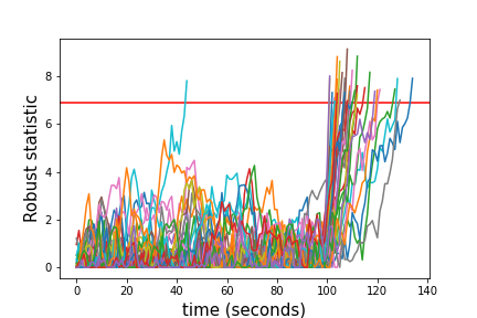
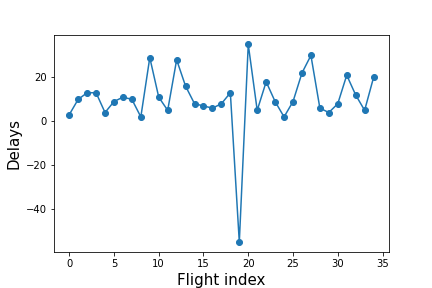
Figure 6: [Left] Robust CUSUM statistic obtained using the pre-change density as $\mathcal{N}(0,1)$ and the post-change as $\mathcal{N}(0.64,1)$. The threshold $6.9=\log(1000)$ is chosen to ensure that the mean time to a false alarm (MFA) is greater than $1000$. [Right] The detection delay profile for the $35$ flights. We saw one false alarm (flight index $19$). The flight arrivals were detected with an average delay of 10.8 seconds over detection paths, i.e., after the false alarm path had been removed.

7.3 Applying Robust CUSUM Test to COVID Infection Data

We now apply the robust CUSUM test to detect the onset of a pandemic. We downloaded the publicly available COVID-19 infection dataset. We selected two U.S. counties, Allegheny and St Louis. The daily number of cases for the first $100$ days are plotted in Fig. 2. The infection rates between the two cities are of similar order since the two cities have similar population sizes. Similar to the Pittsburgh flight data in the previous section, we append the COVID data with zeros and add noise. Since the values are integers, we added $\text{Pois}(1)$ noise; see Fig. 7 (Left) and Fig. 8 (Left). This data generation process simulates the scenario where it is required to detect the onset of a pandemic in the backdrop of daily infections due to other viruses or to detect the arrival of a new variant. Thus, the data represents the detection of deviation from a baseline. Since the actual number of infections is not known and can change over time, we take the robust approach and design the robust test with the LFL given by $\text{Pois}(2)$. The threshold is again chosen to be $6.9=\log(1000)$ to guarantee a mean time to false alarm greater than $1000$ (see (46)). As seen in Fig. 7 (Right) and Fig. 8 (Right), the robust CUSUM test detects the change quickly (within a week) since the infection rates started to become significant (in both counties) after the $70$th day.

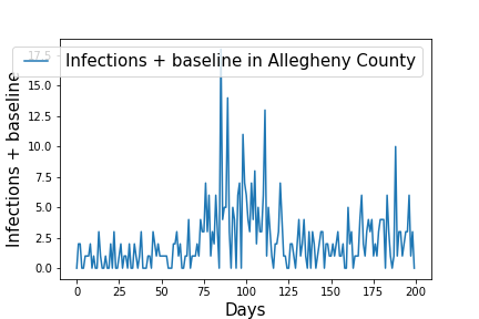
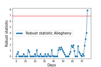
Figure 7: Noisy COVID infection data and robust statistic Allegheny county.

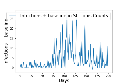
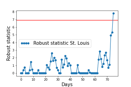
Figure 8: Noisy COVID infection data and robust statistic St. Louis county.

8 Conclusions

We have developed optimal algorithms for the quickest detection of changes from an i.i.d. process to an independent non-stationary process. In most applications of quickest change detection, the post-change law is unknown, and learning it is much harder when the post-change process is also non-stationary. We have shown that if the post-change non-stationary family has a law that is least favorable, then the CUSUM or Shiryaev algorithms designed using the least favorable law (LFL) are robust and optimal. Note that while the LFL itself can be non-stationary, the most interesting case occurs when the LFL is stationary and also i.i.d. The robust optimal solution is then applied to real flight data and COVID-19 pandemic data to detect anomalies.

References

- [1] T. Banerjee, P. Gurram, and G. Whipps, Minimax asymptotically optimal quickest change detection for statistically periodic data, Signal Processing 215 (2024), p. 109290. Available at https://www.sciencedirect.com/science/article/pii/S016516842300364X.
- [2] T. Banerjee, P. Gurram, and G.T. Whipps, A Bayesian theory of change detection in statistically periodic random processes, IEEE Transactions on Information Theory 67 (2021), pp. 2562–2580.
- [3] R. Bansal and P. Papantoni-Kazakos, An algorithm for detecting a change in a stochastic process, IEEE Transactions on Information Theory 32 (1986), pp. 227–235.
- [4] T. Brucks, T. Banerjee, and R. Mishra, Modeling and quickest detection of a rapidly approaching object, To appear in Sequential Analysis (2023).
- [5] V. Krishnamurthy, Partially Observed Markov Decision Processes, Cambridge University Press, 2016.
- [6] T.L. Lai, Information bounds and quick detection of parameter changes in stochastic systems, IEEE Trans. Inf. Theory 44 (1998), pp. 2917 –2929.
- [7] Y. Liang, A.G. Tartakovsky, and V.V. Veeravalli, Quickest change detection with non-stationary post-change observations, IEEE Transactions on Information Theory 69 (2022), pp. 3400–3414.
- [8] G. Lorden, Procedures for reacting to a change in distribution, Ann. Math. Statist. 42 (1971), pp. 1897–1908.
- [9] G.V. Moustakides, Optimal stopping times for detecting changes in distributions, Ann. Statist. 14 (1986), pp. 1379–1387.
- [10] Y. Oleyaeimotlagh, T. Banerjee, A. Taha, and E. John, Quickest change detection in statistically periodic processes with unknown post-change distribution, To appear in Sequential Analysis (2023).
- [11] E.S. Page, Continuous inspection schemes, Biometrika 41 (1954), pp. 100–115.
- [12] J. Patrikar, B. Moon, S. Ghosh, J. Oh, and S. Scherer, TrajAir: A General Aviation Trajectory Dataset (2021). Available at https://kilthub.cmu.edu/articles/dataset/TrajAir_A_General_Aviation_Trajectory_Dataset/14866251.
- [13] M. Pollak, Optimal detection of a change in distribution, Ann. Statist. 13 (1985), pp. 206–227.
- [14] H.V. Poor and O. Hadjiliadis, Quickest detection, Cambridge University Press, 2009.
- [15] A.N. Shiryaev, On optimum methods in quickest detection problems, Theory of Prob and App. 8 (1963), pp. 22–46.
- [16] R.H. Shumway and D.S. Stoffer, Time series analysis and its applications: with R examples, Springer Science & Business Media, 2010.
- [17] A.G. Tartakovsky, I.V. Nikiforov, and M. Basseville, Sequential Analysis: Hypothesis Testing and Change-Point Detection, Statistics, CRC Press, 2014.
- [18] A.G. Tartakovsky and V.V. Veeravalli, General asymptotic Bayesian theory of quickest change detection, SIAM Theory of Prob. and App. 49 (2005), pp. 458–497.
- [19] A. Tartakovsky, Sequential change detection and hypothesis testing: general non-iid stochastic models and asymptotically optimal rules, CRC Press, 2019.
- [20] J. Unnikrishnan, V.V. Veeravalli, and S.P. Meyn, Minimax robust quickest change detection, IEEE Trans. Inf. Theory 57 (2011), pp. 1604 –1614.
- [21] V.V. Veeravalli and T. Banerjee, Quickest Change Detection, Academic Press Library in Signal Processing: Volume 3 – Array and Statistical Signal Processing, 2014.