Abstract

We introduce a simple extensive-form algorithm for finding equilibria of two-player, zero-sum games. The algorithm is realization equivalent to a generalized form of Fictitious Play. We compare its performance to that of a similar extensive-form fictitious play algorithm and a counter-factual regret minimization algorithm. All three algorithms share the same advantages over normal-form fictitious play in terms of reducing storage requirements and computational complexity. The new algorithm is intuitive and straightforward to implement, making it an appealing option for those looking for a quick and easy game solving tool.

1 Introduction

In recent years there has been a great deal of progress in computational methods for solving large games. Interest in the subject stems from both practical applications where AIs, such as self-driving vehicles, interact with each other and humans, and from a handful recreational games, such as chess, poker and Go, that are seen as challenging surrogates for real-world applications, while simultaneously appealing to a large population of devoted enthusiasts. In particular, work on the popular variant of poker known as Texas Hold’em has seen many years of progress culminate in a number of high-profile success stories. Poker and other card games are especially challenging, as they are games with imperfect information and a large number of game states. The development of the Counter-Factual Regret Minimization (CFR) algorithm by Zinkevich, et. al. (?) marked a significant advance in solving large extensive-form games, eventually leading to the numerical solution of the two-player, limit version of Texas Hold’em (?). This was followed by other successful AIs that defeated top professional poker players in heads-up no-limit (?) and multi-player no-limit (?) Texas Hold’em.

It has been recognized from the earliest days of game theory that using behavior strategies is often preferable to mixed strategies for analyzing large games. Despite this, many computational methods use mixtures, $\sigma^{i}(s)$, of pure strategies, $s\in S^{i}$, that specify a specific action to be taken by player $i$ at every game state that player may encounter: $\sum_{s\in S^{i}}\sigma^{i}(s)=1.$ Fictitious Play (FP), for example, is one of the oldest computational methods for solving games (?, ?). In its original formulation, it is a method for finding a Nash Equilibrium (NE) in two-player, zero-sum, normal form games. In this method, the average of the prior play is iteratively updated to

$$\sigma_{n+1}^{i}=\left(1-\frac{1}{n+1}\right)\sigma^{i}_{n}+\frac{1}{n+1}\beta^{i}(\sigma_{n}^{-i}),$$ (1)

where $-i$ indicates player $i$’s opponent, $\beta^{i}(\sigma^{-i}_{n})$ is a best response to the opponent’s play on the previous time-step:

$$\beta^{i}(\sigma^{-i}_{n})\in\arg\max_{\sigma^{i}}u^{i}(\sigma^{i},\sigma^{-i}_{n}),$$ (2)

and $u^{i}(\sigma^{i},\sigma^{-i})$ is expected utility, accounting for the mixed strategies of both players and the role of a chance.

While the normal form of a game is often preferable for analyzing games in general, it balloons the computational cost and amount of storage required for games. In contrast, behavior strategies provide a more compact way of representing a strategy by assigning a distribution, $b(I,a)\geq 0$, over the actions $a\in A(I)$ available at each information set $I\in{\cal I}$:

$$\sum_{a\in A(I)}b(I,a)=1,$$

including those controlled by a chance player, who plays a fixed strategy. When players have perfect recall—they do not forget any information they knew in the past—there exists a strategy of either type equivalent to a given strategy of the other type (?, ?).

The use of behavior strategies was one of the features that allowed the CFR algorithm and its derivatives, like CFR+ (?), to achieve the successes mentioned above. A key advantage of the behavior strategy description lies in being able to consider the expected utility, $U(I,a;b)$, of a specific action, $a\in A(I)$, at a given information set $I$, where the utility is measured from the perspective of the player who controls $I$, and $b$ represents the collection of behavior strategies for all players at all information sets. In what follows, we refer to $U(I,a;b)$ as the action-utility, and suppress $b$ when the strategies are clear from context, writing $U(I,a)\equiv U(I,a;b)$. Similarly, we will use $U(I,{\bf b})\equiv U(I,{\bf b};b)$ to indicate the utility of playing a specific mixture of actions ${\bf b}$ at $I$ that may or may not be consistent with that dictated by $b$.

More recently Heinrich. et. al. (?) develop a version of FP, which they call Extensive-Form Fictitious Play (XFP), that also takes advantage of the efficiency of behavior strategies. In this paper we introduce a similar algorithm that we refer to as Generalized Extensive-Form Fictitious Play (GXFP). In close analogy to FP, GXFP consists of a sequence of behavior strategies:

$$b_{n+1}=\left(1-\frac{1}{n+1}\right)b_{n}+\frac{1}{n+1}d(b_{n}),$$ (3)

where $d(b_{n})$ is the collection of best decisions that are locally optimized with respect to both the opponent’s current strategy and a player’s own current strategy following actions $a\in A(I)$:

$$d(I,*;b_{n})\in\arg\max_{\bf b}U(I,{\bf b};b_{n}).$$ (4)

We will see that GXFP enjoys the same advantages as CFR and XFP in terms of how computational cost and storage scale with the size of the game, but with a simpler and more intuitive implementation. In practice (4) can be be computed by simply selecting the best action, and this mimics the way humans think. In particular, expected value computations for what we have called action utilities are routinely discussed in the recreational poker literature, but to the extent humans can really make these calculations they focus on their immediate decision using their own current strategy and their beliefs about how their opponents play.

In the next section, we briefly review the CFR and XFP algorithms, and further introduce GXFP. In section 3, we show that GXFP is equivalent to a generalized FP, and therefore inherits its convergence properties. In section 4, we discuss a benchmark game that generalizes a classic model of poker put forward by von Neumann and Morgenstern (vN&M) (?). In section 5, we use this benchmark game to compare the performance of the three algorithms. We summarize and conclude in the final section.

2 Algorithms

We start with a description of elements common to all three algorithms considered in this paper, and follow this with a discussion of each algorithm separately.

In games with imperfect information, a player may not know which node he/she is at, and must analyze their decisions based on the probability that their opponent’s prior play has brought them to a particular information set. In comparing the expected value of actions, a player need not consider the probability that their own prior actions will bring them to that information set. Thus the play of a player in any such calculation is assumed to have been consistent with the need to make the decision. For this reason, $U(I,a)$ is referred to as counter-factual utility in (?). This “play-to-reach” assumption is common to all of the algorithms we consider in this paper.

The action-utility can be computed using a basic utility function, ${\cal U}^{i}(\ell)$, defined on the set of leaves in the game tree, the conditional probability of $i$’s opponent’s, including the chance player, playing so as to reach a node $x\in I$ controlled by $i$, and the conditional probability of all players playing so as to reach leaf $\ell$ starting from $I$ with action $a$:

$$U(I,a) = \sum_{x\in I}P^{-i}(x|I)\sum_{\ell\in L_{x,a}}P(\ell|x,a){\cal U}^{i}(\ell),$$ (5)

$$= \sum_{x\in I}\frac{P^{-i}(x)}{P^{-i}(I)}\sum_{\ell\in L_{x,a}}P(\ell|x,a){\cal U}^{i}(\ell),\quad P^{-i}(I)>0,$$ (6)

where the second sum on each line is over leaves, $L_{x,a}$, that can be reached using action $a$ at node $x$.

The various “reach” probabilities can be computed from the behavior strategies $b(I,a)$ and the unique sequence of actions starting at the root of the game tree and terminating at a node $x$: $a^{x}_{1},a^{x}_{2},\dots,a^{x}_{J_{x}}$, where there are $J_{x}$ actions along the path leading to $x$:

$$P^{-i}(x) = \prod_{j=1,I(a_{j}^{x})\notin{\cal I}^{i}}^{J_{x}}b(I(a_{j}^{x}),a_{j}^{x}),$$ (7)

$$P^{-i}(I) = \sum_{x\in I}\prod_{j=1,I(a_{j}^{x})\notin{\cal I}^{i}}^{J_{x}}b(I(a_{j}^{x}),a_{j}^{x}),$$ (8)

$$P(\ell|x,a) = \prod_{j=J_{x}+2}^{J_{\ell}}b(I(a_{j}^{\ell}),a_{j}^{\ell}).$$ (9)

Note that the behavior coefficient for $a$ is omitted in the last product, as the probability is conditioned on that choice.

In the rest of this section, we describe the three algorithms considered in this paper.

2.1 Counter-factual Regret Minimization

The basic version of CFR put forward in (?) is now sometimes referred to as “vanilla” CFR, and is a popular entry point for those getting started with reinforcement learning (RL). While the authors go beyond this version, adapting it to specific features of Texas Hold’em, and there have been subsequent developments, most notably CFR+ (?), we will be considering only this basic version.

CFR is based on the notion of regret for having played the game according to the current strategy $b(I,*)$ rather than taking a specific action $a$ at information set $I$:

$$U(I,a)-U(I,b(I,*)),$$

where

$$U(I,b(I,*))=\sum_{a\in A(I)}b(I,a)U(I,a).$$

More specifically, CFR maintains the average regret, weighted by the opponent’s reach probabilities $P^{-i}(I;b_{n})$:

$$R_{n}(I,a)=\frac{1}{n}\sum_{k=1}^{n}P^{-i}(I;b_{k})\left(U(I,a;b_{k})-U(I,b_{k}(I,*);b_{k})\right).$$ (10)

Notice that the opponent’s reach probability appears as the normalization factor in the computation of the action-utilities, canceling the weighting factor and eliminating the need to compute these quantities unless one actually wishes to compute the utility. At the same time, this removes the possibility of division by zero should $P^{-i}(I)=0$. The strategy at the next iteration is proportional to the amount of positive regret

$$b_{n+1}(I,a)=\left\{\begin{array}[]{ll}\frac{\max(R_{n}(I,a),0)}{\sum\limits_{a\in A(I)}\max(R_{n}(I,a),0)},&\mbox{if}\sum\limits_{a\in A(I)}\max(R_{n}(I,a),0)>0,\\ \frac{1}{|A(I)|},&\mbox{otherwise}.\end{array}\right.$$ (11)

Finally, it is the average of the sequence of strategies $b_{n}(I,a)$, weighted by the reach probability of the player who controls $I$, that converges to a NE:

$$\bar{b}_{n}(I,a) = \frac{\sum_{k=1}^{n}P^{i}(I;b_{k})b_{k}(I,a)}{\sum_{k=1}^{n}P^{i}(I;b_{k})},$$ (12)

$$P^{i}(I) = \prod_{j=1,I(a_{j}^{x})\in{\cal I}^{i}}^{J_{x}}b(I(a_{j}^{x}),a_{j}^{x}),\,\forall x\in I.$$ (13)

2.2 Extensive-Form Fictitious Play

The key advantage of CFR over (normal form) FP is the ability to focus on one information set at a time. As demonstrated by Heinrich et. al. (?), FP can be reformulated so that it too has this feature. They do this by calculating a sequence of behavior strategies that is realization equivalent to the sequence of normal form strategies

$$\sigma^{i}_{n+1}=(1-\alpha_{n+1})\sigma^{i}_{n}+\alpha_{n+1}\beta^{i}(\sigma^{-i}_{n}),$$ (14)

where $\beta^{i}$ is a best response to the opponent’s current strategy $\sigma^{-i}_{n}$. This is a generalized FP with weights $\alpha_{n}$ that decay to zero with a diverging sum $\sum\alpha_{n}=\infty$, and reduces to the classic FP algorithm when $\alpha_{n}=\frac{1}{n}$. Their convergence proof relies on a result of Leslie and Collins (?), who define the following class of generalized fictitious play algorithms, and then proceed to show that any such algorithm converges to a NE of a zero-sum game.

Definition 1.

A generalized weakened fictitious play process is any process $\{\sigma_{n}\}_{n\geq 0}$, with $\sigma_{n}\in\Sigma$, such that

$$\sigma_{n+1}\in\{(1-\alpha_{n+1})\sigma_{n}+\alpha_{n+1}(\beta_{\epsilon_{n}}(\sigma_{n})+M_{n+1})\}_{\beta_{\epsilon_{n}}},$$

where $\beta_{\epsilon_{n}}=(\beta^{1}_{\epsilon_{n}},\beta^{2}_{\epsilon_{n}})$ is in the set of $\epsilon_{n}$-best response vectors, $\alpha_{n}\rightarrow 0$, $\epsilon_{n}\rightarrow 0$ as $n\rightarrow\infty$,

$$\sum_{n\geq 1}\alpha_{n}=\infty,$$

and $\{M_{n}\}_{n\geq 1}$ is a sequence of perturbations such that, for any $T>0$,

$$\lim_{n\rightarrow\infty}\sup_{k}\{||\sum_{j=n}^{k-1}\alpha_{j+1}M_{j+1}||:\sum_{j=1}^{k-1}\alpha_{j+1}\leq T\}=0.$$

Note that in (14), $\epsilon=0$ and $\beta^{i}$ is a best response. Neither XFP nor GXFP make use of $\epsilon$-best responses, and we will later use the $\epsilon$ subscript to indicate a strategy in a perturbed game where actions must be taken with finite probability.

The L&C (?) theorem relies on a result of Benaïm et. al. (?), which we will also need in the following section. We present the theorem in the form given by L&C.

Theorem 1 (Benaïm, et. al.).

Assume $F:\mathbb{R}^{m}\rightarrow\mathbb{R}^{m}$ is a closed set-valued map such that $F(\sigma)$ is a non-empty compact convex subset of $\mathbb{R}^{m}$ with

$$\sup{||z||:z\in F(z)}\leq c(1+||\sigma||)\quad\forall\sigma.$$

Let $\{\sigma_{n}\}_{n\geq 0}$ be the process satisfying

$$\sigma_{n+1}-\sigma_{n}-\alpha_{n+1}M_{n+1}\in\alpha_{n+1}F(\sigma_{n}),$$

with $\alpha_{n}\rightarrow 0$ as $n\rightarrow\infty$,

$$\sum_{n\geq 1}\alpha_{n}=\infty,$$

and $\{M_{n}\}_{n\geq 1}$ be a sequence of perturbations such that, for any $T>0$,

$$\lim_{n\rightarrow\infty}\sup_{k}\{||\sum_{j=n}^{k-1}\alpha_{j+1}M_{j+1}||:\sum_{j=1}^{k-1}\alpha_{j+1}\leq T\}=0.$$

The set of limit points of $\{\sigma_{n}\}$ is a connected internally chain-recurrent set of the differential inclusion

$$\frac{d}{dt}\sigma_{n}\in F(\sigma_{n}).$$ (15)

L&C first show that any GFP (14) satisfies the requirements of this theorem, and then show that the set of limit points is the set of NE.

Theorem 2 (Leslie and Collins).

Any generalized weakened fictitious play process will converge to the set of NE in two-player zero-sum games, potential games, and generic 2 $\times$ 2 games.

Finally, Heinrich et. al. show that the mapping from the normal form strategies (14) to behavior form strategies requires

$$b_{n+1}(I,a)=b_{n}(I,a)+\frac{\alpha_{n+1}P^{i}(I;B^{i}_{n+1})(B^{i}(I,a;b^{-i}_{n})-b_{n}(I,a))}{(1-\alpha_{n+1})P^{i}(I;b_{n}^{i})+\alpha_{n+1}P^{i}(I;B^{i})},$$ (16)

where $B^{i}$ is a best response behavior strategy to $b_{n}^{-i}$:

$$B_{n+1}^{i}\in\arg\max_{b^{i}}u^{i}(b^{i},b_{n}^{-i}),$$ (17)

and $P^{i}$ is player $i$’s reach probability for either the current strategy or the current best response.

When implemented using only (16-17), we found XFP failed to maintain normalized behavior strategies due to the accumulation of round-off error. In some cases this error became so significant that the total exploitability could not be reliably calculated, sometimes giving a negative result. For this reason, we implemented XFP with a renormalization step at each iteration:

$$\hat{b}_{n+1}(I,a)=b_{n+1}(I,a)/\sum_{a}b_{n+1}(I,a),$$ (18)

using $\hat{b}_{n}$ in place of $b_{n}$ in (16).

2.3 Generalized Extensive Form Fictitious Play

While GXFP (3-4) can be implemented with best responses (17) rather than best decisions (4), we found it to be significantly more accurate with the latter, in that the residual exploitability due to round-off error was much smaller. We found the opposite to be true for XFP—it converged with either type of what we will call better responses, but was significantly more accurate with best responses. The convergence proof for GXFP is essentially the same in both cases, with either choice requiring an expansion of Definition 1 to include a weakened notion of better response that will be described in the next section.

In practice (4) can be computed by simply choosing any optimal action:

$$d(I,a;b_{n})=\delta_{a\tilde{a}},\mbox{ where }\tilde{a}\in\arg\max_{a\in I}U(I,a;b_{n}),$$

where $\delta_{a\tilde{a}}$ is the Kronecker delta. This is a much more straigt-forward procedure than computing a best response $B^{i}$, which requires navigating the game tree from the leaves up toward the root.

Finally, GFXP can be implemented with a more general weight $\alpha_{n}$, but we chose to use the simple average of best decisions that can be computed by counting the number of times each action is best at a given information set, thus avoiding the accumulation of round off error. This option, which is not available for CFR and XFP, may be useful for extremely large games.

3 Convergence of Generalized Extensive-Form Fictitious Play

To prove that GXFP converges, we first expand Definition 1 to include alternative “better” responses. We then show that GXFP is equivalent to one of these expanded GFPs. Next, we use Theorem 1 to adapt Theorem 2 to establish convergence. Finally we adapt a theorem due to Hofbauer & Sorin (?) to prove that the attractive set is the set of NE.

We will need the mapping from behavior strategies to mixed strategies:

$$\sigma^{i}(s;b)=\prod_{I\in{\cal I}^{i}}b(I,a(s,I)),$$ (19)

where where $a(s,I)$ is the action $a\in A(I)$ consistent with the pure strategy $s\in S^{i}$. The better response required to show that (3) converges takes the form

$$\tilde{d}^{i}(s;b)=\frac{1}{|{\cal I}^{i}|}\sum_{\bar{I}\in{\cal I}^{i}}d(\bar{I},a(s,\bar{I});b)\prod_{I\neq\bar{I},I\in{\cal I}^{i}}b(I,a(s,I)),$$ (20)

where $d$ is the best decision (4) introduced earlier. Note that $\tilde{d}^{i}$ is a mixed strategy, whereas $d$ is a behavior strategy, and that these depend on the strategy of both opponents. In view of (19), we will use $\tilde{d}^{i}(s;b)\equiv\tilde{d}^{i}(\sigma)$ and $\tilde{d}(\sigma)$ to indicate the better response vector, as we have done with best responses. The proofs given below hold with best responses (17) replacing best decisions to define $\tilde{B}^{i}(s;b_{n})$, but, as noted earlier, we found this to be computationally less accurate.

Theorem 3.

GXFP is realization equivalent to a generalized weakened FP with best responses $\beta_{\epsilon}(\sigma)$ replaced by weakened better decisions $\tilde{d}$.

Proof.

Inserting (4) into the mapping from behavior strategies to mixed strategies gives

$$\sigma_{n+1}^{i}(s;b_{n+1}) = \prod_{I\in{\cal I}^{i}}b_{n+1}(I,a(s,I))$$

$$= \prod_{I\in{\cal I}^{i}}\left[\left(1-\frac{1}{n+1}\right)b_{n}(I,a(s,I))+\frac{1}{n+1}d(I,a(s,I);b_{n})\right].$$

Next, we isolate terms of $O(\frac{1}{n})$ and larger from the product

$$\sigma_{n+1}^{i}(s;b_{n+1}) = \left(1-\frac{|{\cal I}^{i}|}{n+1}\right)\prod_{I\in{\cal I}^{i}}b_{n}(I,a(s,I))$$ (21)

$$+\frac{1}{|{\cal I}^{i}|}\sum_{\bar{I}\in{\cal I}^{i}}\frac{|{\cal I}^{i}|}{n+1}d(\bar{I},a(s,\bar{I});b_{n})\prod_{I\neq\bar{I},I\in{\cal I}^{i}}b_{n}(I,a(s,I))$$

$$+\frac{|{\cal I}^{i}|}{n+1}M^{i}_{n+1}(s;b_{n}),$$

where we have removed a factor of $\frac{|{\cal I}^{i}|}{n+1}$ from the finite number of higher order terms and grouped what remains into the perturbation $M^{i}_{n+1}$. Letting

$$\alpha_{n}=\frac{|{\cal I}^{i}|}{n},$$

and rearranging (21) gives

$$\sigma_{n+1}^{i}\in\{(1-\alpha_{n+1})\sigma_{n}^{i}+\alpha_{n+1}(\tilde{d}^{i}+M^{i}_{n+1})\}_{\tilde{d^{i}}}.$$

The weights $\alpha_{n}$ are proportional to those in standard FP and satisfy the requirements in Definition 1, while the perturbations $M_{n}=(M^{1}_{n},M^{2}_{n})=O\left(\frac{1}{n}\right)$ decay sufficiently fast to ensure the requirement

$$\lim_{n\rightarrow\infty}\sup_{k}\{||\sum_{j=n}^{k-1}\alpha_{j+1}M_{j+1}||:\sum_{j=1}^{k-1}\alpha_{j+1}\leq T\}=0.$$

∎

In the L&C result (?), the relevant differential inclusion is (15). In view of Theorem 3, we must consider instead the weakened better response defined above.

Theorem 4.

The set of limit points of a generalized weakened fictitious play process with best responses $\beta_{\epsilon}(\sigma)$ replaced by weakened better decisions $\tilde{d}$ is a connected internally chain-recurrent set of the differential inclusion

$$\frac{d}{dt}\sigma_{n}\in\{\tilde{d}(\sigma_{n})-\sigma_{n}\}_{\tilde{d}}\equiv F(\sigma_{n}).$$ (22)

Proof.

$F(\sigma)$ satisfies the requirement of Theorem 1:

$$\sup{||z||:z\in F(z)}\leq c(1+||\sigma||)\quad\forall\sigma.$$

The requirements on the perturbation $M_{n}$ in Definition 1 are the same as in Theorem 1, and were already shown to be satisfied in the proof of Theorem 3. ∎

Finally, we must show the attractive set is the set of NE:

Theorem 5.

Any generalized weakened fictitious play process with best responses $\beta_{\epsilon}(\sigma)$ replaced by weakened better decisions $\tilde{d}$ will converge to the set of NE in two-player zero-sum games.

Proof.

We must show that the attractors of the differential inclusion (22) are the set of NE. We will follow the proof of Hofbauer and Sorin (?), who show this for (15). They do this by considering the total exploitability,

$$v(t) = V(\sigma^{1}(t),\sigma^{2}(t))=\max_{\sigma^{1}}u^{1}(\sigma^{1},\sigma^{2})-\min_{\sigma^{2}}u^{1}(\sigma^{1},\sigma^{2})$$ (23)

$$= \sum_{i\in\{1,2\}}u^{i}(\beta^{i}(\sigma^{-i}),\sigma^{-i})\geq 0.$$

They show that $v(t)$ evolving under the best response differential inclusion (15) satisfies

$$\frac{d}{dt}v(t)\leq-v(t),$$

implying

$$v(t)\leq e^{-t}v(0),$$

so that $v(t)$ decays to zero. They also show how to adapt this to the discrete dynamics of a FP process. An unexploitable strategy pair is a NE by definition.

The proof given by Hofbauer & Sorin applies to (22) if we replace the best responses with the weakened better response $\tilde{d}^{i}$:

$$\tilde{v}(t)=\widetilde{V}(\sigma(t))=\sum_{i\in\{1,2\}}u^{i}(\tilde{d}^{i}(\sigma),\sigma^{-i}),$$

as the result ultimately follows from the convexity of $V$, which also holds for $\widetilde{V}$. Thus, their arguments translate to

$$\frac{d}{dt}\tilde{v}(t)\leq-\tilde{v}(t),$$

implying

$$\tilde{v}(t)\leq e^{-t}\tilde{v}(0),$$

with $\tilde{v}(t)$ decaying to zero. When this alternative measure of exploitability $\tilde{v}(t)$ reaches zero there will be no information set at which either player can unilaterally improve. Working backward through the game tree, this implies that both players are playing a best response, hence we are at a NE.

∎

4 Benchmark Game

The analysis of large games is often absent from books on game theory, which tend to focus on extremely simple games, e.g. rock-paper-scissors or the Prisoner’s Dilemma. A notable exception to this occurs in The theory of games and economics behavior by von Neumann and Morgenstern (?), which features an in depth analysis of two models for the game of poker. The text refers to these as the symmetric and asymmetric games. A footnote at the opening of this discussion reveals that these models were largely responsible for von Neumann’s original exploration of game theory. Poker itself is so complicated that few take on the task of using something like Texas Hold’em as a benchmark, so reduced models are often used for the purpose of exploring RL methods. Many of these models can be solved exactly.

Of the two models considered by vN&M, the asymmetric one is more similar to the actual game of poker. Further, it is more challenging from a computational perspective, as it possesses an infinite number of NE. While this is a useful starting point for benchmarking, the game tree is not deep enough for the play-to-reach feature to matter, as neither player has any control over which of their own informaton sets are reached. The game of poker, however, suggests many ways of generalizing this game into a broad family of potential benchmark games that are still relatively easy to implement.

In this section, we first review the results from vN&M for their asymmetric game, and then introduce a generalized version that features a somewhat deeper game tree.

4.1 Von Neumann and Morgenstern’s asymmetric game

The solutions to large games can be bewildering from a human perspective. A further advantage of simplified models is that one can gain some intuitive understanding of how more complicated games work. Starting with vN&M’s asymmetric game will help us understand what is happening in the benchmark game we consider in the next section.

In these two-player zero-sum games, players are ‘dealt’ hands (private information) that take the form of random numbers. The discrete version of these games, where the players are dealt random integers, $1\leq i\leq N$, is mentioned in vN&M, but the text principally focuses on the continuous versions of these games, with hands $x\in[0,1]$. The continuous versions are more readily solved exactly, and the solutions for the asymmetric game closely track that of the discrete game for large $N$. This will be useful for understanding our numerical solutions.

In the asymmetric game, each of the players ante an amount $A$, forming a pot $P=2A$, and then take turns deciding whether or not to place an additional bet $B$. The players are betting on their private information—the value of a random number ‘dealt’ to them after placing their antes, but before making the additional bets. The first player to act may either check (i.e. bet zero) or place a bet of fixed size $B>0$. In the vN&M model, the second player only acts if this bet is placed, and then has the option to fold or call. If the second player folds, the first player receives the antes. If the fist player checks or the second player calls, the pot is distributed according to the highest hand. In their text, vN&M introduce what would later be called a behavior-strategy description of these games, where $b^{i}(x,a)$ describes the fraction of time player $i$ takes action $a$ at each information set. They find this game to have a continuum of optimal solutions (equivalent to NE, which had not yet been invented). The first player plays the same strategy in all of these, having two thresholds between which they never bet, and outside of which they always bet:

$$x_{1} = \frac{AB}{4A^{2}+5AB+B^{2}},$$

$$x_{2} = \frac{2A^{2}+4AB+B^{2}}{4A^{2}+5AB+B^{2}}.$$

The lower region corresponds to a bluff. In the modern recreational poker literature, betting one’s weakest and strongest hands is referred to as betting a polarized range. Despite its simplicity, the model captures this significant insight into poker strategy. The second player has an infinite number of choices that achieve NE. If we let $b^{2}(y,\mbox{call})$ be the fraction of time the second player calls a bet when facing one, vN&M show that

$$\frac{1}{x_{2}-z_{0}}\int_{z_{0}}^{x_{2}}b^{2}(y,\mbox{call})dy\left\{\begin{array}[]{ll}=\frac{A}{A+B}&\mbox{if }\,z_{0}=x_{1}\\ \geq\frac{A}{A+B}&\mbox{if }\,x_{1}<z_{0}<x_{2}\end{array}\right.$$

are both necessary and sufficient conditions for equilibrium. Among these choices, there is a single, weakly-dominant strategy where the second player always folds/calls below/above a threshold

$$y_{1}=\frac{3AB+2B^{2}}{4A^{2}+5AB+B^{2}}.$$

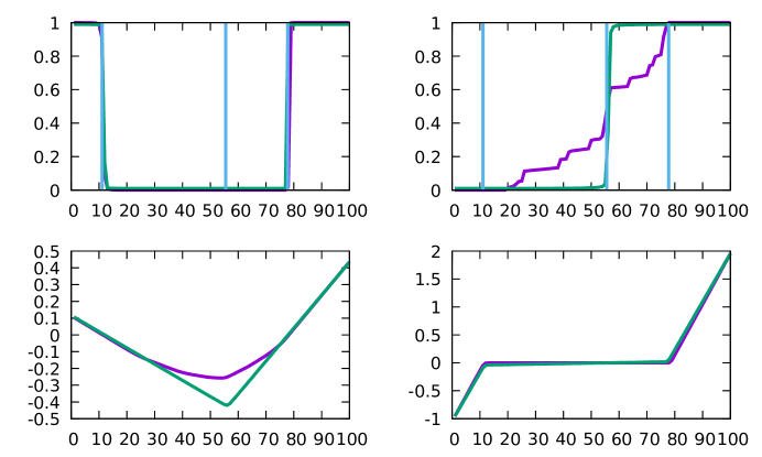
Figure 1: The discrete version of vN&M’s asymmetric game with $P=1,B=1$ and $N=100$ hands. The purple curves correspond to no perturbation, $\epsilon=0$; the green curves are the perturbed game with $\epsilon=0.01$. Top row: the fractions with which player 1 bets (left panel) and player 2 calls (right panel), along with the thresholds for the continuous game (blue vertical lines). Bottom row: the difference in the expected value of player 1’s options (left panel) and player 2’s options (right panel).

Numerical solutions using any of the algorithms described above reveal an analogous result, where player 2’s strategy endlessly drifts among weakly dominated strategies. For this reason, we consider both the perturbed game, where each option at a given information set is played with a minimum probability, $b(I,a)\geq\epsilon$, and the non-perturbed game. This is straightforward with GXFP, as we simply constrain the best decision:

$$d_{\epsilon}(I,a)=\epsilon+(1-\epsilon)\delta_{a\tilde{a}},\mbox{ where }\tilde{a}\in\arg\max_{a\in I}U(I,a;b_{n}).$$ (24)

A similar calculation can be made when computing best responses with XFP, while CFR requires a somewhat more complicated adjustement (?). In Figure 1, we present results for the game with $N=100$ uniformly distributed hands. These results are analogous to those shown vN&M.

The graphs in the top row are the fractions with which player 1 bets (left panel) and player 2 calls (right panel). For player 1, the unperturbed result (shown in purple) and the perturbed result with $\epsilon=0.01$ (shown in green) are nearly indistinguishable, indicative of there being a unique strategy for player 1 at equilibrium. For comparison, the thresholds given above for the continuous version of the game are shown as blue vertical lines. For player 2, the perturbed result is unique and approximates the solution with pure-strategy thresholds given above, while the unperturbed result endlessly drifts among the set of NE that employ a weakly-dominated strategy for player 2.

In the bottom row of Figure 1, we graph the difference in the expected value of player 1’s options (left panel) and player 2’s options (right panel), with a positive difference corresponding to the betting and calling options, respectively. From the left panel, we see that player 2’s weakly dominated strategy is outperformed by the dominant one if player 1 is forced to bet with probability $\epsilon$ in the region where the unperturbed strategy is to check. Examining the lower-right panel, we see that there is no significant difference in player 2’s perturbed and unperturbed payoff, as player 1 plays a nearly equal strategy in each case. We also see that the ambivalence in player 2’s strategy is due to being indifferent between calling and folding throughout the region where mixed equilibria exist.

4.2 The benchmark game

If one understands fictitious play to mean finding the average best response to an opponent’s prior play, and does not realize this was originally only considered for the normal form of a game, it is easy to stumble upon algorithm (3-4). The situation is more subtle, however, if the game tree is deeper. This requires the play-to-reach assumption. This issue is irrelevant in the case of the game just discussed. To bring it to the forefront, we will consider a slightly more complicated version of the asymmetric game that allows for a bet and a single raise, including the possibility of a check-raise. This game is briefly addressed in Chen & Ankenman (?), a book aimed primarily at recreational poker players, but the discussion omits the details given below.

For the continuous version of the game, a NE using pure-action choices containing 12 thresholds exists, but the strategy for player 1 is weakly dominated by an infinite number of other stategies, including pure-action strategies that features two additional thresholds. This differs from what happens in the vN&M game, where there is a unique pure-action NE with the smallest number of thresholds and weakly dominant strategies. For the expanded game just described, the linear system of equations that would determine the full set of thresholds is singular, leading to a degeneracy of pure action equilibria. The numerical results presented in the next section reveal that this game also features an infinite number of mixed strategy NE, with this occurring for both players.

When the pot $P=2A=1$, bet $B=1$ and raise $R=1$, the eight thresholds for player 1 are $\{x_{1}=64/1083,x_{2}=369/722,x_{3}=10/19,x_{4}=x_{5}-32/1083,x_{5},x_{6}=307/361,x_{7}=x_{8}-22/361,x_{8}\}$, where $x_{5}$ and $x_{8}$ can be chosen arbitrarily so long as all of the thresholds remain in ascending order. These correspond to nine intervals of hands where player 1 takes a specific sequence of actions: $\{\mbox{bet-fold}<\mbox{check-fold}<\mbox{check-raise}<\mbox{check-call}<\mbox{bet-fold}<\mbox{check-call}<\mbox{bet-call}<\mbox{check-raise}<\mbox{bet-call}\}$. The six thresholds for the second player divide into two sets of three: $\{y_{1}^{1}=8/57,y_{2}^{1}=41/57,y_{3}^{1}=15/19\}$, corresponding to four intervals where player 2 responds to a check with the actions $\{\mbox{bet-fold}<\mbox{check}<\mbox{bet-fold}<\mbox{bet-call}\}$ and $\{y_{1}^{2}=1/2,y_{2}^{2}=10/19,y_{3}^{2}=17/19\}$ where player 2 responds to a bet with the actions $\{\mbox{fold}<\mbox{raise}<\mbox{fold}<\mbox{call}\}$.

5 Numerical experiments

As with the asymmetric game, the degeneracy of the solution means that the numerical solution will drift among the possible equilibria. This makes direct comparison of the strategy profiles generated by the methods difficult. Thus in our first figure in this section we present only a single realization generated by GXFP. The CFR and XFP algorithms give qualitatively similar results, as do other initial conditions. In the rest of the section we will be able to make direct comparisons.

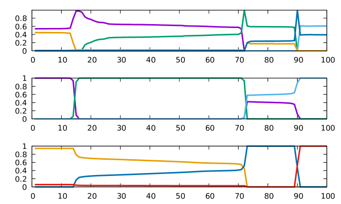
Figure 2: Numerical solution of the benchmark game with $P=1,B=1,R=1$ and $N=100$ hands. Top panel: the probability with which player one takes the action sequences check-fold (purple), check-call (green), check-raise (light blue), bet-call (dark blue), and bet-fold (gold). Middle panel: player 2’s response to an initial check from player 1: either check (green), bet-fold (purple), or bet-call (light blue). Bottom panel: player 2’s response to an initial bet from player 1: either fold (gold), call (dark blue), or raise (red).

In Figure 2 we plot the strategies returned by the GXFP algorithm as a function of the hand strength, $1\leq i\leq 100$. In the top panel, the purple curve is the probability of checking, followed by folding to a bet; the green curve is the probability of checking, followed by calling a bet, and the light blue curve is the probability of checking, followed by raising, these three quantities adding to one. The remaining two strategy sequences, bet-call (dark blue) and bet-fold (gold) also add to one. The middle panel is player 2’s response to an initial check from player 1: either another check (green), a bet followed by a fold if raised (purple), or a bet followed by a call if raised (light blue), these three quantities adding to one. The bottom panel is player 2’s response to an initial bet from player 1: either fold (gold), call (red), or a raise (dark blue), with these three quantities again adding to one. The main thing to notice here is that there is a mixture of strategies being used for most hands, indicative of the type of degeneracy we saw in the asymmetric game, only this time it occurs for both players.

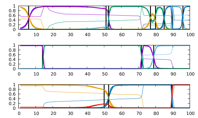
Figure 3: Numerical solution of the perturbed ($\epsilon=0.01$) benchmark game using XFP and GXFP (nearly identical; both using the color scheme described in the last figure) and the unperturbed ($\epsilon=0.0$) benchmark game using GXFP (all blue, thin line) for $P=1,B=1,R=1$, and $N=100$, along with the thresholds (black vertical lines) for the continuous version of the game.

As with the asymmetric game, we find that we can again remove the weakly dominated strategies by approximating the equilibria subject to a small perturbation. The results for doing this with XFP and GXFP are shown in Figure 3, along with the unperturbed solution from Figure 2 and the thresholds for the continuous version of the game. The two arbitrary thresholds ($x_{5}$ and $x_{8}$) were roughly fit to these graphs, but the fit of all other thresholds provides a useful way of detecting coding errors. The mixing near the thresholds is due to boundary effects inherent to the discrete game, and diminishes as the number of possible hands increases. Some of these regions are very narrow, so the discretization affects the result more strongly. The results for the two algorithms are nearly identical, as expected. We did not adapt CFR to play the perturbed game.

To make comparisons between all three algorithms, we examine plots of the utility of the current strategy pair $u^{1}(b_{n}^{1},b_{n}^{2})$ measured from player 1’s perspective and the total exploitability $v(t)\geq 0$, defined in equation (23). In principal, the former should converge to the value of the game, but in practice there is some numerical error due to finite precision arithmetic. The total exploitability serves as a measure of this error.

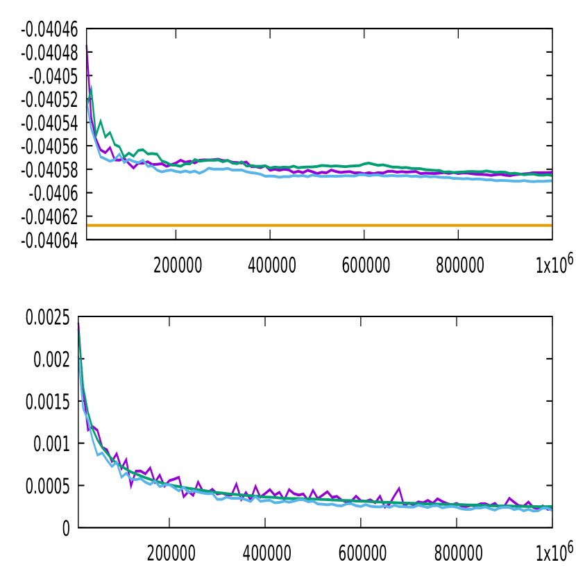
Figure 4: Numerical solution of the benchmark game with $P=1,B=1,R=1$, and $N=100$ hands. Top panel: the value of the game (from player 1’s perspective) returned by the three algorithms at intervals of $10,000$ iterations, along with the exact value for the continuous version of the game, $-\frac{44}{1083}\approx 0.406$, shown in gold. A sample for each of the of the algorithms is shown for random initial data: GXFP in purple, CFR in light blue and XFP in green. Bottom panel: the corresponding plots for total exploitability.

In the top panel of Figure 4 we plot the expected value of the current strategy pair (from player 1’s perspective) returned by the three algorithms at intervals of $10,000$ iterations, along with the the exact value of $-\frac{44}{1083}\approx 0.406$ for the continuous version of the game, shown in gold. A sample for each of the three algorithms is shown for random initial data. The solutions oscillate somewhat at the scale shown, but are all comparable in magnitude. Results vary with initial conditions, but are qualitatively similar. The numerical solutions will get closer to the solution for the continuous version of the game as $N\rightarrow\infty$, but round off error will prevent them from achieving this solution exactly.

While getting the correct value of the game is desirable, this can sometimes be achieved with nonoptimal strategies. A better measure of error is the total exploitability. In the lower panel, we plot this quantity at every $10,000$ iterations for the same samples presented in the top panel. The error and the rate at which it decays is similar for all three methods.

Finally, we should note that all three algorithms have a similar computational cost per iteration, despite the somewhat more complicated XFP and CFR recursive updates. The extra calculations needed to compute regret or a best response scale with the number of information sets, $|{\cal I}^{1}|+|{\cal I}^{2}|$, but the most expensive part of these calculations, computing the action utilities, must be done for all three algorithms, and this scale like $|{\cal I}^{1}||{\cal I}^{2}|$.

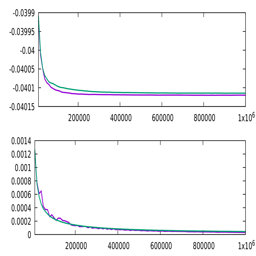
Figure 5: The perturbed ($\epsilon=0.01$) benchmark game with $P=1,B=1,R=1$, and $N=100$ hands. Top panel: the value of the game (from player 1’s perspective) returned at intervals of $10,000$ iterations. A sample of each algorithm is shown for random initial data: GXFP in purple and XFP in green. Bottom panel: the corresponding plots for total exploitability.

In Figure 5, we compare the performance of XFP and GXFP for generalized NE with $\epsilon=0.01$. In the top panel, the purple and green curves are once again the utility of the current strategy pair from player 1’s perspective returned by the GXFP and XFP algorithms at intervals of $10,000$ iterations. The bottom panel is the exploitability using the same color scheme. Note that convergence for the perturbed game is much faster than for the unperturbed one, a result of the degenerate NE making convergence much more difficult to achieve.

6 Summary

In this work we have introduced a new algorithm, GXFP, that is realization equivalent to a generalized form of Fictitious Play, thus inheriting the convergence properties of that class of algorithms. We then compared the computational performance of GXFP to that of two additional algorithms, CFR and XFP, using an expanded version of a simple poker model first introduced by von Neumann and Morgenstern. This benchmark game, where each of the two players makes at least one, and up to two, decisions, has a somewhat deeper game tree that requires the play-to-reach utilities that are common to all three algorithms. We also presented an exact solution for the continuous version of this game that is useful for testing the algorithms. Like vN&M’s original game, this game features an infinite number of NE. As a result, a variation of the game with a perturbed strategy space and a unique equilibrium was also considered. This generalized NE is computed more quickly and is easier to interpret.

The computational cost per iteration is comparable for all three algorithms. GXFP’s simple update formula requires no best response calculation, relying instead on a best decision calculation that is intuitive and, at least in some approximate sense, routinely used to make decisions in recreational games. This makes it an ideal choice for anyone looking for a quick and easy game solving tool. Unlike the other two algorithms, GXFP can be implemented without accumulating round-off by using integer type variables to count the number of times a strategy choice was best. This can be done with or without the perturbed strategy space. GXFP also has somewhat lower memory requirements. These features may be helpful for solving especially large games.

Finally, all three algorithms converged much more quickly when using updates that alternate between the two players, using the opponent’s most recently updated strategy rather than the strategy from the previous iteration. This is a well-known feature of algorithms of this type, and is, for example, largely responsible for CFR+’s faster convergence (?, ?).

References

- Benaim et al. Benaim, M., Hofbauer, J., & Sorin, S. (2005). Stochastic approximations and differential inclusions. SIAM J. Contol Optim., 328–348.
- Bowling et al. Bowling, M., Burch, N., Johanson, M., & Tammelin, O. (2015). Heads-up limit hold’em poker is solved. Science, 145–149.
- Brown Brown, G. W. (1949). Some Notes on Computation of Games Solutions. RAND Corporation.
- Brown & Sandholm Brown, N., & Sandholm, T. (2018). Superhuman ai for heads-up no-limit poker: Libratus beats top professionals. Science, 418–424.
- Brown & Sandholm Brown, N., & Sandholm, T. (2019). Superhuman ai for multiplayer poker. Science, 885–890.
- Burch et al. Burch, N., Moravcik, M., & Schmid, M. (2019). Revisiting cfr+ and alternating updates. J. of Artificial Intelligece Research, 429–443.
- Chen & Ankenman Chen, B., & Ankenman, J. (2006). The Mathematics of Poker. Conjelco.
- Farina et al. Farina, G., Kroer, C., & Sandholm, T. (2017). Regret minimization in behaviorally-constrained zero-sum games. In Proc. of the 34th International Conference on Machine Learning.
- Heinrich et al. Heinrich, J., Lanctot, M., & Silver, D. (2015). Fictitious self-play in extensive-form games. In Proc. of the 32nd International Converence on Machine Learning.
- Hofbauer & Sorin Hofbauer, J., & Sorin, S. (2006). Best response dynamics for continuous zero-sum games,. Discrete and Continuous Dynamical Systems B, 215–224.
- Kuhn Kuhn, H. (1953). Extensive games and the problem of information. In Contributions to the Theory of Games, Vol. II, Annals of Mathematical Studies No. 28.
- Leslie & Collins Leslie, D., & Collins, E. (2006). Generalized weakened fictitious play. Games and Economic Behavior, 285–298.
- Maschler et al. Maschler, M., Solan, E., & Zamir, S. (2013). Game Theory,”. Cambridge.
- Robinson Robinson, J. (1951). An iterative method of solving a game. Annals of Math., 296–301.
- Tammelin Tammelin, O. (2014). Sovling large imperfect information games using cfr+. In Corr.
- von Neuman & Morgenstern von Neuman, J., & Morgenstern, O. (1944). Theory of Games and Economic Behavior. Princeton University Press.
- Zinkevich et al. Zinkevich, M., Johanson, M., Bowling, M., & Piccione, C. (2008). Regret minimization in games wth incomplete information. Advances in Neural Information Processing Systems, 20, 906–912.