DPZero: Private Fine-Tuning of Language Models
without Backpropagation

Abstract

The widespread practice of fine-tuning large language models (LLMs) on domain-specific data faces two major challenges in memory and privacy. First, as the size of LLMs continues to grow, the memory demands of gradient-based training methods via backpropagation become prohibitively high. Second, given the tendency of LLMs to memorize training data, it is important to protect potentially sensitive information in the fine-tuning data from being regurgitated. Zeroth-order methods, which rely solely on forward passes, substantially reduce memory consumption during training. However, directly combining them with standard differentially private gradient descent suffers from growing model size. To bridge this gap, we introduce DPZero, a novel private zeroth-order algorithm with nearly dimension-independent rates. The memory efficiency of DPZero is demonstrated in privately fine-tuning RoBERTa on six downstream tasks.

1 Introduction

Fine-tuning pretrained large language models (LLMs), including BERT [26, 76, 100], OPT [137], LLaMA [112, 113], and GPT [96, 13, 92, 91], achieves state-of-the-art performance in a wide array of downstream applications. However, two significant challenges persist in practical adoption: memory demands for gradient-based optimizers and the need to safeguard the privacy of domain-specific fine-tuning data.

As the memory requirement of fine-tuning LLMs is increasingly becoming a bottleneck, various approaches have been proposed, spanning from parameter-efficient fine-tuning (PEFT) [65, 54] to novel optimization algorithms [20, 70]. Since these methods rely on backpropagation to compute the gradients, which can be memory-intensive, a recent trend has emerged in developing algorithms that do not require backpropagation [10, 105, 52, 53, 94, 18]. Specifically for LLMs, Malladi et al. [82] introduced zeroth-order methods for fine-tuning, thereby eliminating the backward pass and freeing up the memory for gradients and activations. Utilizing a single A100 GPU, zeroth-order methods are capable of fine-tuning a 30-billion-parameter model, whereas first-order methods, even equipped with PEFT, fails to fit into the memory for a model with more than 6.7 billion parameters. This greatly expands the potential for deploying and fine-tuning LLMs even on personal devices.

On the other hand, empirical studies have highlighted the risk of LLMs inadvertently revealing sensitive information from their fine-tuning datasets [86, 133, 85, 80]. Such privacy concerns are pronounced especially when users opt to fine-tune LLMs on datasets of their own. Notably, the expectation that machine learning models should not compromise the confidentiality of their contributing entities is codified into legal frameworks [116]. Differential privacy (DP) [30] is a widely accepted mathematical framework for ensuring privacy by preventing attackers from identifying participating entities [104]. Consequently, the development of methods that fine-tune LLMs under differential privacy is of pressing necessity [67, 130, 51, 15, 27, 109]; however, most efforts so far have focused on first-order algorithms.

Motivated by the memory-hungry nature and privacy concerns in fine-tuning LLMs, we investigate zeroth-order methods that guarantee differential privacy for solving the following stochastic optimization problem:

$$\min_{x\in\mathbb{R}^{d}}F_{S}(x)\;:=\;\frac{1}{n}\sum_{i=1}^{n}f(x;\xi_{i})\;,$$ (1)

where $S=\{\xi_{i}\}_{i=1}^{n}$ is the training data, $x\in\mathbb{R}^{d}$ is the model weight, the loss $f(x;\xi_{i})$ is Lipschitz for each sample $\xi_{i}$, and the averaged loss $F_{S}(x)$ is smooth and possibly nonconvex. In theory, previous work on both differentially private optimization [7] and zeroth-order optimization [29] indicate that their convergence guarantees depend explicitly on the dimension $d$. Such dimension dependence becomes problematic in the context of LLMs with $d$ scaling to billions. In practice, and somewhat surprisingly, empirical studies on the fine-tuning of LLMs using zeroth-order methods [82] and DP first-order methods [130, 67, 66] have shown that the performance degradation due to the large model size is marginal. For example, Yu et al. [130] showed that the performance drop due to privacy is smaller for larger architectures. A 345 million-sized GPT-2-Medium, fine-tuned with ($\varepsilon=6.8,\delta=10^{-5}$)-DP, showcases a modest drop of 5.1 in BLEU score [93] (compared to a non-private model of the same size and architecture), whereas a larger GPT-2-XL with 1.5 billion parameters exhibits smaller cost in test performance, i.e., 4.3 BLEU score under the same privacy budget.

This gap between theory and practice has been linked to the presence of low-rank structures in the fine-tuning of pretrained LLMs [82, 66]. Empirical evidence suggests that fine-tuning occurs within a low-dimensional subspace [98, 49, 42, 64]: 200 dimensions for RoBERTa with 355 million parameters [2] and 100 dimensions for PEFT on DistilRoBERTa with 7 million parameters [66]. In such cases where the intrinsic dimension is small, zeroth-order methods are known to achieve dimension independent convergence rate [82] and private first-order methods are also known to achieve dimension independent guarantees [81, 66].

Given the significance of fine-tuning LLMs on domain-specific datasets, we ask the following fundamental question: Can we achieve a dimension-independent rate both under differential privacy and with access only to the zeroth-order oracle? Our contributions are summarized below.

$\bullet$ We first show that the straightforward approach–that combines DP first-order methods with zeroth-order gradient estimators (Algorithm 1)–exhibits an undesirable dimension-dependence in the convergence guarantees, even when the effective rank of the problem does not scale with the dimension (Theorem 1 and 2 in Section 3). There are two root causes. First, the standard practice of choosing the clipping threshold to be the maximum norm of the estimated sample gradient leads to an unnecessarily large threshold. Next, this choice of the clipping threshold forces the addition of a large noise to ensure privacy, and Algorithm 1 adds that noise in all $d$ directions.

$\bullet$ We present DPZero (Algorithm 2), the first nearly dimension-independent DP zeroth-order method for stochastic optimization. Its convergence guarantee depends on the effective rank of the problem (specified in Assumption 3.5) and exhibits logarithmic dependence on the dimension $d$ (Theorem 3 in Section 4). This builds upon two insights. First, the direction of the estimated gradient is a public information and does not need to be private; it is sufficient to make only the magnitude of the estimated gradient private, which is a scalar value. Next, we introduce a tighter analysis that allows us to choose a significantly smaller clipping threshold, leveraging the fact that the typical norm of the estimated gradient is much smaller than its maximum.

$\bullet$ We verify the effectiveness of DPZero in both synthetic examples and private fine-tuning tasks on RoBERTa [76]. In contrast to first-order algorithms that demand extensive effort for the efficient implementation of per-sample gradient clipping [67, 51, 15], DPZero offers the advantage of near-zero additional costs compared to non-private zeroth-order methods [82]. Our empirical results validate theoretical findings, revealing only a slight performance decrement for DPZero even with large model sizes.

After the workshop version of our paper [136] was released, Tang et al. [110] concurrently discovered the same algorithm as DPZero (up to a minor difference in how $u_{t}$ is drawn) and showed empirical benefits when applied to fine-tuning OPT models [137] but without any theoretical analysis.

1.1 Related Works

We build upon exciting advances in zeroth-order optimization and differentially private optimization, which we survey here. Notably, DPZero is inspired by new empirical and theoretical findings showing that fine-tuning LLMs does not suffer in high-dimensions when using zeroth-order methods in Malladi et al. [82] or using private first-order optimization in Li et al. [66]. A more comprehensive overview is deferred to Appendix A.

Zeroth-order optimization.

Nesterov and Spokoiny [89] pioneered the formal analysis of the convergence rate of zeroth-order methods, i.e., zeroth-order (stochastic) gradient descent (ZO-SGD) that replaces gradients in SGD by their zeroth-order estimators. Their findings are later refined by several works [41, 101, 69]. These well-established results indicate a runtime complexity $\mathcal{O}(d)$ worse than first-order methods. Such dimension-dependence of zeroth-order methods is proven inevitable without additional structures [124, 29].

There are several recent works that relax the dimension-dependence in zeroth-order methods leveraging problem structures. Balasubramanian and Ghadimi [6] demonstrated that ZO-SGD can directly identify the sparsity of the problem and proved dimension-independent rate when the support of gradients remains unchanged [16]. Yue et al. [131], Malladi et al. [82] relaxed the dependence on dimension $d$ to a quantity related to the trace of the loss’s Hessian.

Differentially private optimization.

Previous works on DP optimization mostly center around first-order methods. When the problem is nonconvex, i.e., the setting of our interest, differentially private (stochastic) gradient descent (DP-GD) achieves a rate of $\mathcal{O}(\sqrt{d\log(1/\delta)}/(n\varepsilon))$ on the squared norm of the gradient [120, 139]. We show that DPZero matches this rate with access only to the zeroth-order oracle in Theorem 3. Given access to the first-order oracle, it has been recently shown that such rate can be improved to $\mathcal{O}((\sqrt{d\log(1/\delta)}/(n\varepsilon))^{4/3})$ leveraging momentum [114] or variance reduction techniques [3].

Early works established dimension-independent rates when the gradients lie in some fixed low-rank subspace [56, 108]. Closest to our result is Song et al. [108], which demonstrated that the rate of DP-GD for smooth nonconvex optimization can be improved to $\mathcal{O}(\sqrt{r\log(1/\delta)}/(n\varepsilon))$ for generalized linear models (GLMs) with a rank-$r$ feature matrix. DPZero matches this result with access only to the zeroth-order oracle in Theorem 3 for more general problems beyond low-rank GLMs. Our result is inspired by Li et al. [66] that introduced a relaxed Lipschitz condition for the gradients and provide dimension-free bounds when the loss is convex and the relaxed Lipschitz parameters decay rapidly. Similarly, Ma et al. [81] suggested that the dependence on $d$ in the utility upper bound for DP stochastic convex optimization can be improved.

Literature on DP optimization beyond first-order methods remains notably limited. As far as we are aware, no prior studies have addressed the challenge of deriving a dimension-independent rate in DP zeroth-order optimization.

2 Preliminaries

Notation.

We use $\lVert\cdot\rVert$ for the Euclidean norm and define $\|v\|_{W}^{2}=v^{\top}Wv$ for a square matrix $W$. $\mathbb{S}^{d-1}=\{x\in\mathbb{R}^{d}\,|\,\lVert x\rVert=1\}$ denotes the unit sphere in $\mathbb{R}^{d}$, and $\eta\,\mathbb{S}^{d-1}$ is the sphere of radius $\eta>0$. A function $p:\mathbb{R}^{d}\rightarrow\mathbb{R}$ is $L$-Lipschitz if $\lvert p(x_{1})-p(x_{2})\rvert\leq L\lVert x_{1}-x_{2}\rVert,\forall x_{1},x_{2}$. A function $q:\mathbb{R}^{d}\rightarrow\mathbb{R}$ is $\ell$-smooth if it is differentiable and $\lVert\nabla q(x_{1})-\nabla q(x_{2})\rVert\leq\ell\lVert x_{1}-x_{2}\rVert$. The trace of a square matrix $J$ is denoted by $\,\text{Tr}(J)$. A symmetric real matrix $M\succeq 0$ if it is positive semi-definite. The clipping operation is defined to be $\,\text{clip}_{C}(x)=x\,\min\{1,C/\lVert x\rVert\}$ given $C>0$. The notation $\tilde{\mathcal{O}}(\cdot)$ hides additional logarithmic terms.

2.1 Differential Privacy

Definition 2.1 (Differential Privacy [30, 31]).

Two datasets $S=\{\xi_{i}\}_{i=1}^{n}$ and $S^{\prime}=\{\xi_{i}^{\prime}\}_{i=1}^{n}$ are neighboring if $\max\{|S\setminus S^{\prime}|,|S^{\prime}\setminus S|\}=1$ and we denote it by $S\sim S^{\prime}$. For prescribed $\varepsilon>0$ and $\delta\in(0,1)$, an algorithm $\mathcal{A}$ is said to be $(\varepsilon,\delta)$-differential privacy (DP) if $\mathbb{P}(\mathcal{A}(S)\in B)\leq e^{\varepsilon}\mathbb{P}(\mathcal{A}(S^{\prime})\in B)+\delta$ for all $S\sim S^{\prime}$ and all measurable set $B$ in the range of $\mathcal{A}$.

To ensure DP while solving the optimization problem in Eq. (1), first-order approaches, such as DP-GD, update via $x_{t+1}\leftarrow x_{t}-\alpha((1/n)\sum_{i=1}^{n}{\rm clip}_{C}(\nabla f(x_{t};\xi_{i}))+z_{t})$; see e.g., [107, 1]. Through the following composition lemma [58, Theorem 4.3], the per-sample clipping operation that ensures finite sensitivity of $\Delta=2C/n$ together with the Gaussian noise $z_{t}$ secure the privacy for entire $T$ updates.

Lemma 2.2 (Advanced Composition).

Let $\mathcal{A}$ be some randomized algorithm operating on a dataset $S$ and outputting a vector in $\mathbb{R}^{d}$. If $\mathcal{A}$ has sensitivity $\Delta:=\sup_{S\sim S^{\prime}}\lVert\mathcal{A}(S)-\mathcal{A}(S^{\prime})\rVert$, the mechanism that adds Gaussian noise $\mathcal{N}(0,\sigma^{2}\mathrm{I}_{d})$ with variance $\sigma^{2}=(2\Delta\sqrt{2T\log(e+(\varepsilon/\delta))}/\varepsilon)^{2}$ satisfies $(\varepsilon,\delta)$-DP under $T$-fold adaptive composition for any $\varepsilon>0$ and $\delta\in(0,1)$.

2.2 Zeroth-Order Optimization

When the gradient is expensive to compute, zeroth-order methods are useful for optimizing Eq. (1). For example, the two-point gradient estimator below requires only two evaluation of function values [101]

$$g_{\lambda}(x;\xi_{i})\;\;:=\;\;\frac{f(x+\lambda u;\xi_{i})-f(x-\lambda u;\xi_{i})}{2\lambda}u\;,$$ (2)

where $u$ is sampled uniformly from the Euclidean sphere $\sqrt{d}\,\mathbb{S}^{d-1}$ and $\lambda>0$ is the smoothing parameter [129, 28]. A common approach to generate $u$ is to set $u=\sqrt{d}\,z/\lVert z\rVert$, with $z$ sampled from the standard multivariate Gaussian $\mathcal{N}(0,\mathrm{I}_{d})$ [87, 84]. We refer to $g_{\lambda}(x;\xi)$ as the zeroth-order gradient (estimator) in the sequel. The results in this paper can be directly extended to other zeroth-order gradient estimators, e.g., any $u$ satisfying $\mathbb{E}[uu^{\top}]=\mathrm{I}_{d}$ [29], the one-point estimators [36], and the directional derivative [89].

3 DP-GD with Zeroth-Order Gradients Suffers in High Dimensions

In this section, we show that the direct integration of zeroth-order gradient estimators Eq. (2) into DP-GD, which we term DPGD-0th, leads to undesirable dimension dependence in the error rate, which persists even under a low effective rank assumption.

3.1 Direct Integration Leads to an ${\cal O}(d^{3/2})$ Rate

We present in Algorithm 1 the straightforward private zeroth-order approach that substitutes the gradient in DP-GD with zeroth order estimators $g_{\lambda}(x_{t};\xi_{i})$ in Eq. (2).

Algorithm 1 DP-GD with 0th-order gradients (DPGD-0th)

0:  Dataset $S=\{\xi_{1},\cdots,\xi_{n}\}$, initialization $x_{0}\in\mathbb{R}^{d}$, number of iterations $T$, stepsize $\alpha>0$, smoothing parameter $\lambda>0$, clipping threshold $C>0$, privacy parameters $\varepsilon>0,\delta\in(0,1)$.

1:  for $t=0,1,\cdots,T-1$ do

2:     Sample $u_{t}$ uniformly at random from the Euclidean sphere $\sqrt{d}\,\mathbb{S}^{d-1}$.

3:     for $i=1,\cdots,n$ do

4:        Compute the zeroth-order gradient estimator

$$g_{\lambda}(x_{t};\xi_{i})\;\leftarrow\;\frac{f(x_{t}+\lambda u_{t};\xi_{i})-f(x_{t}-\lambda u_{t};\xi_{i})}{2\lambda}u_{t}.$$

5:     Sample $z_{t}\in\mathbb{R}^{d}$ randomly from the multivariate Gaussian distribution $\mathcal{N}(0,\sigma^{2}\mathrm{I}_{d})$ with variance $\sigma=4C\sqrt{2T\log(e+(\varepsilon/\delta))}/(n\varepsilon)$ and update the parameter

$$x_{t+1}\;\leftarrow\;x_{t}-\alpha\left(\frac{1}{n}\sum_{i=1}^{n}\,\text{clip}_{C}(g_{\lambda}(x_{t};\xi_{i}))+z_{t}\right).$$

5:  $x_{\tau}$ for $\tau$ sampled uniformly at random from $\{0,1,\cdots,T-1\}$.

The privacy guarantee follows from standard DP-GD analysis, and the utility guarantee on the squared gradient norm is derived from classical techniques for analyzing zeroth-order methods [89]. Before presenting the convergence result, we make the following standard assumption, which is common in nonconvex DP optimization [120, 121, 114].

Assumption 3.1.

The loss $f(x;\xi)$ is $L$-Lipschitz for every $\xi$. The average loss $F_{S}(x)$ is $\ell$-smooth for every given dataset $S$, and its minimum $F_{S}^{*}:=\min_{x\in\mathbb{R}^{d}}F_{S}(x)$ is finite.

Theorem 1.

For any $\varepsilon>0$ and $\delta\in(0,1)$, Algorithm 1 is $(\varepsilon,\delta)$-DP. Under Assumption 3.1, its output $x_{\tau}$ satisfies that

$$\mathbb{E}[\lVert\nabla F_{S}(x_{\tau})\rVert^{2}]\;\;\leq\;\;16\Big{(}(F_{S}(x_{0})-F_{S}^{*})\,\ell+2L^{2}\Big{)}\frac{d\sqrt{d\log(e+(\varepsilon/\delta))}}{n\varepsilon},$$ (3)

with the choice of parameters

$$\alpha=\frac{1}{4\ell d},\quad T=\frac{n\varepsilon}{\sqrt{d\log(e+(\varepsilon/\delta))}},\quad\lambda\leq\frac{4L}{\ell d}\left(\frac{\sqrt{d\log(e+(\varepsilon/\delta))}}{n\varepsilon}\right)^{1/2},\quad C=Ld.$$

The total number of zeroth-order gradient computations is $nT=\mathcal{O}(n^{2}/\sqrt{d})$.

Remark 3.2.

Theorem 1 demonstrates that directly combining DP-GD with zeroth-order gradients leads to an ${\cal O}(d^{3/2})$ error complexity, which is $\mathcal{O}(d)$ worse than first-order DP approaches [120].

Remark 3.3.

Three sources contribute to the dependence in $d$: the squared norm of the zeroth-order gradient estimator $\mathbb{E}[\|(1/n)\sum_{i=1}^{n}g_{\lambda}(x,\xi_{i})\|^{2}]=\mathcal{O}(d\,\lVert\nabla F_{S}(x)\rVert^{2})$ when taking $\lambda\rightarrow 0$ for simplicity, the clipping threshold $C=\mathcal{O}(d)$, and the norm of the privacy noise $\mathbb{E}[\|z_{t}\|^{2}]=\mathcal{O}(d\,C^{2})=\mathcal{O}(d^{3})$. The standard analysis of one-step update gives

$$\mathbb{E}[F_{S}(x_{t+1})]\;\leq\;\mathbb{E}[F_{S}(x_{t})]-\frac{\alpha}{2}\big{(}1-2d\,\ell\alpha\big{)}\,\mathbb{E}[\lVert\nabla F_{S}(x_{t})\rVert^{2}]+c\,\alpha^{2}\,d^{3},$$ (4)

where $c$ is a constant that depends on problem parameters other than $\alpha$ and $d$; see Eq. (12) for details. A small enough step size, $\alpha<1/(2\ell d)$, is required to make the second term negative, where the dependence in $d$ comes from $\mathbb{E}[\|(1/n)\sum_{i=1}^{n}g_{\lambda}(x,\xi_{i})\|^{2}]$. The dependence on $d^{3}$ in the last term arises from $\mathbb{E}[\|z_{t}\|^{2}]$, which leads to the $\mathcal{O}(d^{3/2})$ rate in Eq. (3) after balancing error terms. Detailed proofs can be found in Appendix D.

Remark 3.4.

The choice of the clipping threshold $C=Ld$ ensures that clipping does not happen with probability one, which is a common choice in the theoretical analysis of private optimization algorithms [7, 8, 120]. This follows from the fact that, for $L$-Lipschitz $f(x;\xi)$, the zeroth-order gradient is upper bounded by $\lVert g_{\lambda}(x;\xi)\rVert\leq Ld$ almost surely. Selecting the clipping threshold without knowledge of this upper bound remains an active research topic [22, 128, 33, 62, 138].

3.2 Rate Improves to $\mathcal{O}(d)$ under Low Effective Rank

Here, under the low-dimensional structures in fine-tuning LLMs (cf. Section 1), we demonstrate improved performance for Algorithm 1. Unfortunately, a linear dependence in $d$ still persists even under the low effective rank structure.

Assumption 3.5.

The function $f(x;\xi)$ is $L$-Lipschitz and $\ell$-smooth for every $\xi$. The average function $F_{S}(x)$ is twice differentiable with $-H\preceq\nabla^{2}F_{S}(x)\preceq H$ for any $x\in\mathbb{R}^{d}$, and its minimum $F_{S}^{*}:=\min_{x\in\mathbb{R}^{d}}F_{S}(x)$ is finite. Here, the real-valued $d\times d$ matrix $H\succeq 0$ satisfies that $\lVert H\rVert_{2}\leq\ell$ and $\,\text{Tr}(H)\leq r\lVert H\rVert_{2}$. We refer to $r$ as the effective rank or the intrinsic dimension of the problem.

Assumption 3.5 boils down to Assumption 3.1 if $r=d$. This is because $-H^{\prime}\preceq\nabla^{2}F_{S}(x)\preceq H^{\prime},\forall\,x\in\mathbb{R}^{d}$ and $H^{\prime}=\ell\,\mathrm{I}_{d}$ imply that $\lVert H^{\prime}\rVert_{2}\leq\ell$ and $\,\text{Tr}(H^{\prime})\leq d\lVert H^{\prime}\rVert_{2}$. With $r<d$, this assumption reflects the additional structures encoded in the Hessian matrix. While Assumption 3.5 naturally holds for low-rank Hessians, it covers more general cases. For example, the assumption is satisfied with $r=\mathcal{O}(\log d)\ll d$ in the case of a full-rank matrix $H$, with its $i$-th largest eigenvalue being $\ell/i$ for $1\leq i\leq d$.

Similar assumptions have been made to successfully relax the dimension-dependence in zeroth-order optimization in the limit $\lambda\to 0$ [82] and also for DP first-order optimization when the objective is smooth and convex [81]. However, even under Assumption 3.5, DPGD-0th (Algorithm 1) still suffers from a linear dependence in $d$ in its error rate, as presented below, with a proof in Appendix D.

Theorem 2.

For any $\varepsilon>0$ and $\delta\in(0,1)$, Algorithm 1 is $(\varepsilon,\delta)$-DP. Under Assumption 3.5, its output $x_{\tau}$ satisfies that

$$\mathbb{E}[\lVert\nabla F_{S}(x_{\tau})\rVert^{2}]\;\;\leq\;\;16\Big{(}(F_{S}(x_{0})-F_{S}^{*})\,\ell+2L^{2}\Big{)}\frac{d\sqrt{r\log(e+(\varepsilon/\delta))}}{n\varepsilon},$$ (5)

with the choice of parameters

$$\alpha=\frac{1}{4\ell(r+2)},\quad T=\frac{n(r+2)\varepsilon}{d\sqrt{r\log(e+(\varepsilon/\delta))}},\quad\lambda\leq\frac{4L}{\ell d}\left(\frac{\sqrt{r\log(e+(\varepsilon/\delta))}}{n\varepsilon}\right)^{1/2},\quad C=Ld.$$

The total number of zeroth-order gradient computations is $nT=\mathcal{O}(n^{2}\sqrt{r}/d)$.

Remark 3.6.

Comparing to Remark 3.3, both the zeroth-order gradient, $\mathbb{E}[\lVert(1/n)\sum_{i=1}^{n}g_{\lambda}(x_{t};\xi_{i})\rVert_{H}^{2}]$, and the DP noise, $\mathbb{E}[\lVert z_{t}\rVert_{H}^{2}]$, decrease by a factor of ${\cal O}(r/d)$ under low effective rank. This is made precise in Lemma C.1. As a result, the one-step update analysis can be tightened as

$$\mathbb{E}[F_{S}(x_{t+1})]\;\leq\;\mathbb{E}[F_{S}(x_{t})]-\frac{\alpha}{2}\big{(}1-2(r+2)\ell\alpha\big{)}\,\mathbb{E}[\lVert\nabla F_{S}(x_{t})\rVert^{2}]+c\,\alpha^{2}\,r\,d^{2}.$$ (6)

Comparing to the RHS of Eq. (4), it achieves an improved $d$ dependence. However, the third term in Eq. (6) is still at $\mathcal{O}(d^{2})$ due to the clipping threshold $C=\mathcal{O}(d)$. Consequently, even when the effective rank $r$ is small, Eq. (5) still grows linearly in $d$.

4 DPZero: Nearly Dimension-Independent Differentially Private Zeroth-Order Optimization

A straightforward combination of DP-GD and zeroth-order methods has a large dimension dependence. Our novel DPZero overcomes this issue with two key insights elaborated below.

Algorithm 2 DPZero

0:  Dataset $S=\{\xi_{1},\cdots,\xi_{n}\}$, initialization $x_{0}\in\mathbb{R}^{d}$, number of iterations $T$, stepsize $\alpha>0$, smoothing parameter $\lambda>0$, clipping threshold $C>0$, privacy parameters $\varepsilon>0,\delta\in(0,1)$.

1:  for $t=0,1,\cdots,T-1$ do

2:     Sample $u_{t}$ uniformly at random from the Euclidean sphere $\sqrt{d}\,\mathbb{S}^{d-1}$.

3:     for $i=1,\cdots,n$ do

4:        Compute the finite difference $f(x_{t}+\lambda u_{t};\xi_{i})-f(x_{t}-\lambda u_{t};\xi_{i})$.

5:     Sample $z_{t}\in\mathbb{R}$ randomly from the univariate Gaussian distribution $\mathcal{N}(0,\sigma^{2})$ with variance $\sigma=4C\sqrt{2T\log(e+(\varepsilon/\delta))}/(n\varepsilon)$ and update the parameter

$$x_{t+1}\;\leftarrow\;x_{t}-\alpha\left(\frac{1}{n}\sum_{i=1}^{n}\,\text{clip}_{C}\left(\frac{f(x_{t}+\lambda u_{t};\xi_{i})-f(x_{t}-\lambda u_{t};\xi_{i})}{2\lambda}\right)+z_{t}\right)u_{t}.$$

5:  $x_{\tau}$ for $\tau$ sampled uniformly at random from $\{0,1,\cdots,T-1\}$.

Scalar privacy noise.

By decoupling zeroth-order gradient Eq. (2) into direction and magnitude, our key observation is that the direction, $u_{t}$, is public knowledge, and we only need to make the magnitude private. Privacy can be guaranteed by clipping the finite-difference, $(f(x_{t}+\lambda u_{t};\xi_{i})-f(x_{t}-\lambda u_{t};\xi_{i}))/(2\lambda)$, and then adding a scalar noise $z_{t}$; see line 6 of Algorithm 2. This change, when applied to Algorithm 1, can significantly improve the rate in Eq. (5) by $d^{1/2}$.

Tighter clipping threshold.

Another factor of $d^{1/2}$ improvement originates from a tighter analysis on the upper bound of the finite-difference term. Although its worst-case upper-bound scales with the dimension $d$, this only happens with an exponentially small probability over the randomness of $u_{t}$. As proved in Eq. (16) in Appendix E, the size of the finite-difference is

$$\frac{\lvert f(x_{t}+\lambda u_{t};\xi_{i})-f(x_{t}-\lambda u_{t};\xi_{i})\rvert}{2\lambda}\;\leq\;\lvert u_{t}^{\top}\nabla f(x_{t};\xi_{i})\rvert+\frac{\ell}{2}\lambda d,$$

where we use the assumption that each $f(x;\xi)$ is $\ell$-smooth. When $u_{t}$ is sampled from the sphere $\sqrt{d}\,\mathbb{S}^{d-1}$, a tail bound (part $(ii)$ of Lemma C.1 in the appendix) implies that

$$\mathbb{P}\left(\left\lvert u_{t}^{\top}\nabla f(x_{t};\xi_{i})\right\rvert\geq C\right)\leq 2\sqrt{2\pi}\,\exp\left(-\frac{C^{2}}{8L^{2}}\right).$$

By selecting the smoothing parameter $\lambda$ to be sufficiently small, a careful choice of $C=\tilde{\mathcal{O}}(L)$, which is nearly independent of $d$, can ensure that clipping does not occur with a high probability. This choice is significantly smaller than the worst-case clipping threshold of $Ld^{1/2}$. The main technical challenge is that we need to analyze the algorithm given the event that clipping does not happen. The choice of drawing $u_{t}$ from the uniform distribution over the sphere, together with corresponding tail bounds in Appendix C, allows us to prove the following nearly dimension-independent bound under the low effective rank structure in Assumption 3.5. A proof is provided in Appendix E.

Theorem 3.

For any $\varepsilon>0$ and $\delta\in(0,1)$, Algorithm 2 is $(\varepsilon,\delta)$-DP. Under Assumption 3.5, its output $x_{\tau}$ satisfies that

$$\mathbb{E}[\lVert\nabla F_{S}(x_{\tau})\rVert^{2}]\;\;\leq\;\;\left(64\left((F_{S}(x_{0})-F_{S}^{*})\,\ell+\tilde{L}^{2}\right)+2L^{2}\right)\frac{\sqrt{r\log(e+(\varepsilon/\delta))}}{n\varepsilon},$$ (7)

where we define

$$\tilde{L}^{2}=L^{2}\,\log\left(\frac{2\sqrt{2\pi}\,d(r+2)n^{3}\varepsilon^{2}}{r\log(e+(\varepsilon/\delta))}\right),$$

and choose the parameters to be

$$\alpha=\frac{1}{4\ell(r+2)},\quad T=\frac{n(r+2)\varepsilon}{4\sqrt{r\log(e+(\varepsilon/\delta))}},\quad C=4\tilde{L},$$

$$\lambda\leq\frac{1}{\ell d}\min\left\{4(2-\sqrt{2})\tilde{L},\;\frac{L}{\sqrt{d}}\left(\frac{\sqrt{r\log(e+(\varepsilon/\delta))}}{n\varepsilon}\right)^{1/2}\right\}.$$

The total number of zeroth-order gradient computations is $nT=\mathcal{O}(n^{2}\sqrt{r})$.

Remark 4.1.

Algorithm 2 is nearly dimension-independent, given its logarithmic dependence on $d$. To the best of our knowledge, this is the first zeroth-order DP method that is nearly dimension-independent. This feature is significantly beneficial for fine-tuning pretrained LLMs where the effective rank has been observed to be quite small [2, 66]. When $r=d$, our rate in Eq. (7) nearly matches that of the best known achievable bound of the first-order method DP-GD for smooth nonconvex losses [120]. When the effective rank $r$ is smaller, this algorithm achieves $\tilde{\mathcal{O}}(\sqrt{r\log(1/\delta)}/(n\varepsilon))$ squared gradient norm. Similar dimension-free error rate is established for DP-GD on unconstrained generalized linear losses [108], with a dependence on the rank of the feature matrix. Table 1 provides a summary on how DPZero depends on dimension $d$ and effective rank $r$.

Table 1: The dependence of the error rate on dimension $d$ and effective rank $r$ shows that the proposed DPZero (Alg. 2) significantly outperforms DPGD-0th (Alg. 1) and achieves performance close to the popular first-order method, DP-GD, on both scenarios with and without a low-effective rank assumption. Note that the error rates of zeroth and first-order DP methods are achieved with different number of iterations.

	w/o Asmp. 3.5	with Asmp. 3.5
DPGD-0th	$\mathcal{O}(d\sqrt{d})$	$\mathcal{O}(d\sqrt{r})$
DPZero	$\mathcal{O}((\log d)\sqrt{d})$	$\mathcal{O}((\log d)\sqrt{r})$
DP-GD	$\mathcal{O}(\sqrt{d})$	$\mathcal{O}(\sqrt{r})$

Remark 4.2.

The RHS of Eq. (7) improves upon Eq. (5) of Algorithm 1 by a factor of $d$. Simplifying our analysis in Eq. (22) and conditioning on the event that the clipping does not happen, we get a similar one-step update analysis as Eq. (6) (see Eq. (22) for a precise inequality). However, since the privacy noise $z_{t}$ is a scalar and the clipping threshold has been reduced, we have that $\mathbb{E}[\|z_{t}u_{t}\|_{H}^{2}]=\tilde{\mathcal{O}}(r)$ is nearly independent of the dimension $d$, and thus the final error scales as $\tilde{\mathcal{O}}(r^{1/2})$.

Remark 4.3.

The strategy of appropriately selecting the clipping threshold to ensure that clipping occurs with low probability is commonly applied in the analysis of private algorithms [33, 103]. Adaptive choices of clipping thresholds can provably improve error rates for certain problems including PCA [74] and linear regression [75]. One technical challenge in the choice of the clipping threshold in DPZero is that we need the expected one-step progress to be sufficient in Eq. (22). This requires controlling the progress in the low-probability event that finite difference is clipped. The fact that $\|u_{t}\|$ is finite with probability one simplifies the analysis, which is the reason we choose to sample $u_{t}$ uniformly at random over the sphere. We believe that the analysis extends to the commonly used spherical Gaussian random vectors with more in-depth analysis, which we leave as a future research direction. Table 5 in the appendix supports our hypothesis that the resulting performances are similar whether we use Gaussian or spherical random vectors.

Remark 4.4.

Our theoretical results, including Theorems 1, 2, and 3, can be extended to the setting where the average loss $F_{S}(x)$ additionally satisfies the PL inequality [60, 95, 77]. Under Assumption 3.5, DPZero converges to an optimal solution in a nearly dimension-independent error rate. See more details in Appendix F.

Remark 4.5.

Besides the dimension-free error rates and memory saving of no backpropagation, another practical merit of DPZero stems from the significantly simplified clipping compared with DP-GD. Because only scalar function value difference is clipped, DPZero avoids the memory and runtime overhead for (per-datum) gradient clipping in first order DP approaches [67, 51, 15]. This makes DPZero highly preferable especially in resource-constrained scenarios.

5 Experiments

We provide empirical results on synthetic problems and private fine-tuning of language models for sentence classification tasks. A thorough description of the experimental settings is available in Appendix B. All experiments are tested on a single NVIDIA GeForce RTX 3090 GPU with 24 GiB memory.

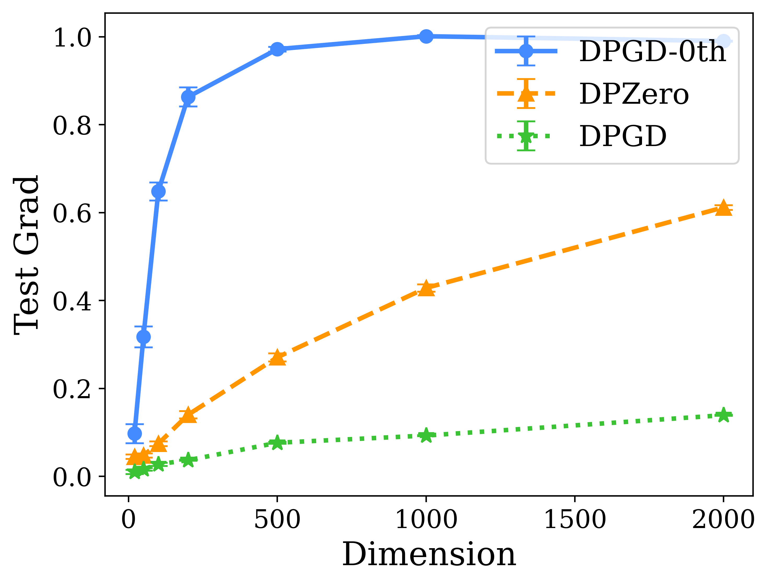
(a) $\,\text{Tr}(A)=\mathcal{O}(d)$.

(b) $\,\text{Tr}(A)=\mathcal{O}(\sqrt{d})$.

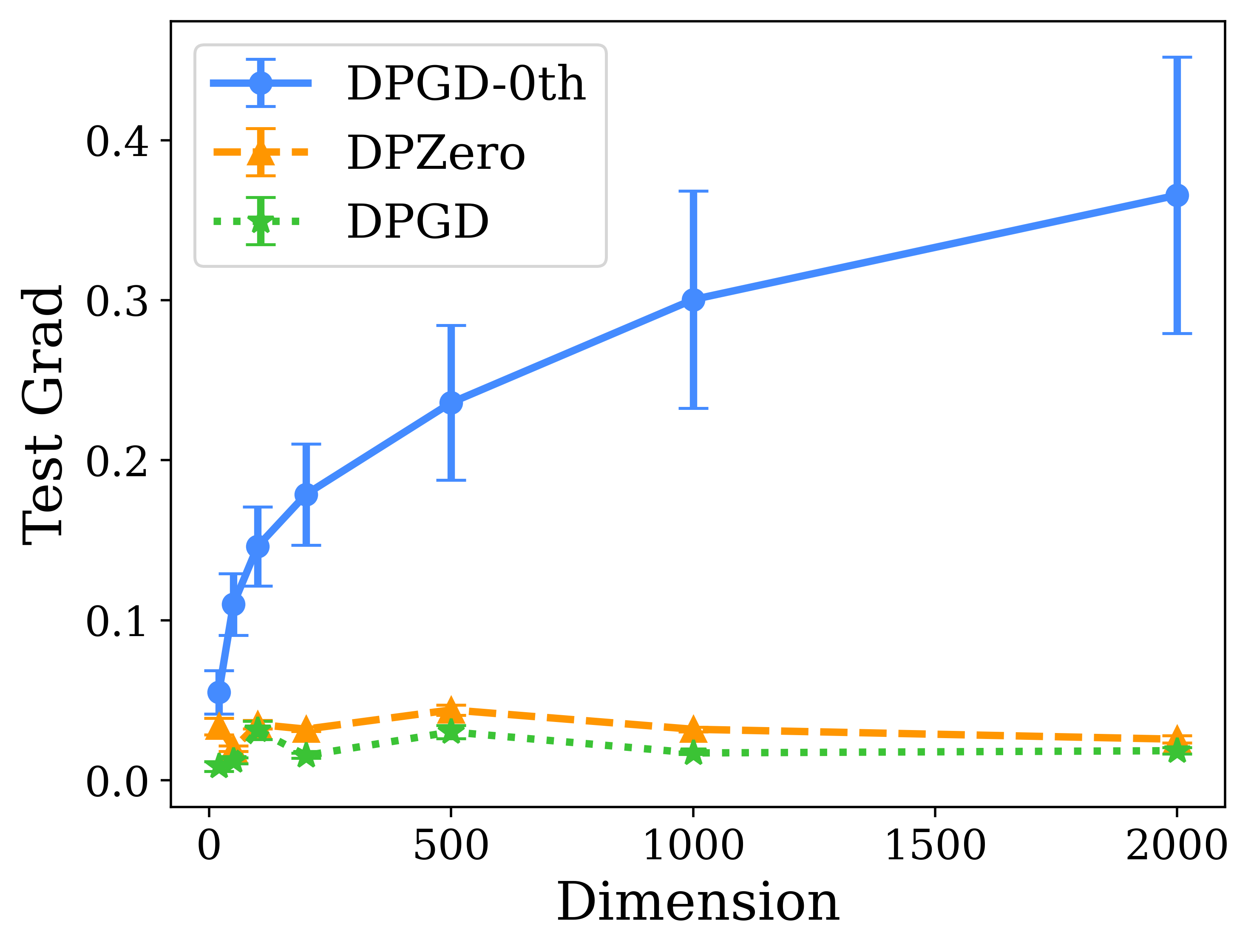
(c) $\,\text{Tr}(A)=\mathcal{O}(\log d)$.

Figure 1: Experiments on the quadratic loss with effective rank $\,\text{Tr}(A)$ (Assumption 3.5). For three different modes of the effective rank, we demonstrate how the norm of the test gradient depends on the problem dimension. DPGD-0th (Algorithm 1) has a strong dimension dependence regardless of the effective rank, while DPZero (Algorithm 2) achieves dimension independent performance when effective rank is small (right panel), similar to the standard first-order method DP-GD.

Synthetic example.

Our first evaluation compares the performance of Algorithm 2 (DPZero) with Algorithm 1 (DPGD-0th) and DP-GD on problems with different effective ranks. In particular, we use a quadratic loss

$$\min_{x\in\mathbb{R}^{d}}F_{S}(x)=\frac{1}{2n}\sum_{i=1}^{n}(x-x_{i})^{\top}A(x-x_{i}),$$

with three choices of the Hessian matrix, $A$, whose effective ranks are designed to be ${\cal O}(d)$, ${\cal O}(\sqrt{d})$, and ${\cal O}(\log d)$, respectively. All methods are trained with $(\varepsilon=2,\delta=10^{-6})$-DP on a training set $\{x_{1},\cdots,x_{n}\}$ with $n=10,000$ and evaluated on a test set of the same size. The problem dimension is increased from 20 to 2,000. We perform a parameter search and plot the best gradient norm evaluated on the test set in Figure 1.

Every method scales with the dimension $d$ when the effective rank is $d$ (as in Figure 1(a)), and DPGD-0th has the worst performance. When the effective rank reduces to $\log d$ (as in Figure 1(c)), both DP-GD and DPZero become nearly dimension-independent, which validates the dimension independence of DPZero. Appendix B.1 includes more results measuring the loss and the gradient norm for both training and test datasets.

Table 2: Experiments on RoBERTa (355M). We report both mean and standard error of the accuracy (%) across three random seeds. MeZO is not private and serves as an upper bound. The zero-shot results with no fine-tuning, taken from Malladi et al. [82], provide lower bounds, since they can be achieved with no private data.

Task	SST-2	SST-5	SNLI	MNLI	RTE	TREC
	—— Sentiment ——		—— Natural Language Inference ——			— Topic —
MeZO	$92.5\pm 0.3$	$50.8\pm 0.8$	$80.4\pm 0.6$	$69.2\pm 0.3$	$72.8\pm 1.0$	$88.9\pm 0.1$
DPZero ($\varepsilon=6$)	$92.2\pm 0.3$	$49.3\pm 0.6$	$77.8\pm 1.0$	$67.4\pm 0.3$	$71.9\pm 0.9$	$87.6\pm 0.9$
DPZero ($\varepsilon=2$)	$91.8\pm 0.1$	$47.1\pm 0.9$	$73.6\pm 0.9$	$62.7\pm 0.9$	$70.4\pm 0.7$	$82.0\pm 1.6$
Zero-Shot	79.0	35.5	50.2	48.8	51.4	32.0

Table 3: Accuracy (%), runtime per iteration (s), and memory consumption (MiB) when fine-tuning RoBERTa (355M) for SST-2. DPZero is as memory and time efficient as a non-private zeroth order method MeZO [82] and achieves accuracy within 1% while ensuring $(\varepsilon=2,\delta=10^{-5})$-DP. Comparing with first-order methods, AdamW [78] and DP-AdamW [130], the benefit of zeroth-order methods is greater for private algorithms, thanks to simpler clipping.

Method	Acc.	Time	Memory
AdamW	94.4	0.425	16960
DP-AdamW	92.3	2.33	21494
MeZO	92.5	0.345	2668
DPZero	91.8	0.347	2668

Language model fine-tuning.

Next, we follow the experimental setting in Malladi et al. [82] and evaluate DPZero on fine-tuning RoBERTa [76] with 355M parameters across six different sentence classification tasks. We consider the few-shot scenario with 512 samples per class. We report the test accuracy for DPZero trained with $(\varepsilon=\{2,6\},\delta=10^{-5})$-DP and non-private zeroth-order baseline MeZO [82] in Table 2. DPZero enjoys the same benefit as MeZO on memory efficiency and achieves near-zero additional costs, with at max only 2.6% drop in the accuracy when $\varepsilon=6$. The memory consumption and per-iteration runtime are shown in Table 3. We note that a rigorous comparison of the total runtime with first-order DP methods is challenging as it depends on the implementation. The total time taken by DP-AdamW (implemented by Yu et al. [130]) and DPZero (implemented by us) are similar as DP-AdamW requires 1,000 iterations while DPZero requires 10,000 iterations. This aligns with Theorem 3, which states that DPZero requires $\mathcal{O}(r)$ times more iterations than DP-GD to attain the same level of error rate, where $r$ is the effective rank.

Compared with first-order DP methods, the main benefit of DPZero is memory efficiency. Such memory savings are even greater than those observed in non-DP domains, due to DPZero’s efficient per-sample clipping. In our experiments, we notice that the clipping threshold of DPZero is typically larger compared to DP first-order methods; see Figure 4 in the appendix. This is also consistent with the results in Theorem 3 regarding the selection of the clipping threshold $C$. Our results confirm that privately fine-tuning pretrained LLMs with the zeroth-order method DPZero does not suffer in high dimensions.

6 Conclusion

DPZero is proposed to privately fine-tune language models in a memory efficient manner by avoiding backpropagation. Theoretically, DPZero enjoys a provably near dimension-free rate under low-rank structures, clearing the barriers for scaling private fine-tuning of LLMs. When deploying DPZero, the elimination of gradient computation not only significantly saves memory, but avoids the overhead in gradient clipping as well. Thus the benefit of using zeroth-order method is more significant for private optimization. The theoretical guarantees on scalability and the practical merits of DPZero are validated on private fine-tuning of RoBERTa.

DPZero uses the full batch gradient every iteration, and the analysis guarantees an upper bound on the empirical average gradient assuming smooth nonconvex objectives. We defer extensions to the stochastic mini-batch setting, guarantees on the population loss leveraging the stability of zeroth-order methods [90], and considerations of other assumptions on objective functions like convexity or nonsmoothness to future research. We believe this work opens up a plethora of other prospective directions in DP zeroth-order optimization. These include, but are not limited to, understanding the advantages of the intrinsic noise in zeroth-order gradient estimators, discovering other structural assumptions like the restricted Lipschitz condition [66] for dimension-independent rates, and utilizing momentum [114] or variance reduction [3] techniques for an improved rate and computational complexity.

Broader Impact

A major concern with current use-cases of large language models is privacy of the fine-tuning data. Fine-tuning on in-domain data greatly improves performance and is now a default option. However, in-domain data can contain sensitive information about the participants of the dataset. The proposed solution makes privacy protection easier, consuming less resources, thus democratizing the use of privacy enhancing technology beyond those who have access to large amounts of resources.

Appendix A Additional Related Works

Zeroth-order optimization.

Nesterov and Spokoiny [89] pioneered the formal analysis of the convergence rate of zeroth-order methods, i.e., zeroth-order (stochastic) gradient descent (ZO-SGD) that replaces gradients in SGD by their zeroth-order estimators. This is motivated by renewed interest in adopting zeroth-order methods in industry due to, for example, fast differentiation techniques that require storing all intermediate computations reaching the memory limitations. Their findings on nonsmooth convex functions are later refined by Shamir [101]. Lin et al. [69] contributed to further advancements on nonsmooth nonconvex functions recently. Additionally, Ghadimi and Lan [41] extended the results for smooth functions into the stochastic setting. Zeroth-order methods have also been expanded to incorporate approaches such as coordinate descent [68], conditional gradient descent [6], variance reduction techniques [71, 32, 57], SignSGD [72], and minimax optimization [123]. Additionally, zeroth-order methods find applications in fields such as black-box machine learning [46, 19, 21], bandit optimization [36, 101], reinforcement learning [99, 23, 83], and distributed learning [34, 132, 127] to reduce communication overhead. These well-established results indicate that the norm of the zeroth-order gradient scales with the dimension $d$ and the required stepsize is $d$-times smaller than that in first-order gradient-based methods, leading to a $d$-times increase in the final time complexity. For example, the convergence rate of gradient descent for minimizing a smooth convex function $f(x)$ is $f(\bar{x}_{T})-\min_{x\in\mathbb{R}^{d}}f(x)\leq\mathcal{O}(1/T)$ where $\bar{x}_{T}$ is the average of $T$ iterates [88], while the zeroth-order method only achieves a rate $\mathcal{O}(d/T)$. It has been shown that such dimension-dependence of zeroth-order methods is inevitable without additional structures [124, 29].

There are several recent works that relax the dimension-dependence in zeroth-order methods leveraging problem structures. Wang et al. [122] and Cai et al. [16] assumed certain sparsity structure in the problem and applied sparse recovering algorithms, e.g. LASSO, to obtain sparse gradients from zeroth-order observations. Golovin et al. [44] analyzed the case when the objective function is $f(Px)$ for some low-rank projection matrix $P$. These works either require the objective or the algorithm to be modified to have a dimension-independent guarantee. Balasubramanian and Ghadimi [6] demonstrated that ZO-SGD can directly identify the sparsity of the problem and proved dimension-independent rate when the support of gradients remains unchanged [16]. Recently, Yue et al. [131], Malladi et al. [82] relaxed the dependence on dimension $d$ to a quantity related to the trace of the loss’s Hessian.

Differentially private optimization.

Previous works on DP optimization mostly center around first-order methods. For constrained convex problems, tight utility guarantees on both excess empirical [17, 7, 126, 134, 120] and population [8, 9, 35, 4, 63, 135] losses are well-understood. As an example, a typical result states that the optimal rate on the excess empirical loss for convex objectives is $\Theta(\sqrt{d\log(1/\delta)}/(n\varepsilon))$, where $(\varepsilon,\delta)$ are privacy parameters, $n$ is the number of samples, and $d$ is the dimension. The dimension-dependence is fundamental as both the upper bound [7], using differentially private (stochastic) gradient descent (DP-GD) introduced in [107], and the lower bound [7], using a reduction to finger printing codes, have the same dependence.

When the problem is nonconvex, i.e., the setting of our interest, DP-GD achieves a rate of $\mathcal{O}(\sqrt{d\log(1/\delta)}/(n\varepsilon))$ on the squared norm of the gradient [120, 139]. We show that DPZero matches this rate with access only to the zeroth-order oracle in Theorem 3. Given access to the first-order oracle, it has been recently shown that such rate can be improved to $\mathcal{O}((\sqrt{d\log(1/\delta)}/(n\varepsilon))^{4/3})$ leveraging momentum [114] or variance reduction techniques [3]. Further, the convergence to second-order stationary points in nonconvex DP optimization is studied in [39]. Recent advancements in DP optimization have also delved into the understanding of the potential of public data [37, 79], the convergence properties of per-sample gradient clipping [128, 33, 62, 138], and the relaxation of the dimension-dependence in the utility upper bound [81, 66].

Early works established that dimension-independent rates can be attained when the gradients lie in some fixed low-rank subspace [56, 108]. By first identifying this gradient subspace, dimension-independent algorithms can be designed [140, 59]. Closest to our result is Song et al. [108], which demonstrated that the rate of DP-GD for smooth nonconvex optimization can be improved to $\mathcal{O}(\sqrt{r\log(1/\delta)}/(n\varepsilon))$ under certain structural assumptions, i.e., for generalized linear models (GLMs) with a rank-$r$ feature matrix. DPZero matches this result with access only to the zeroth-order oracle in Theorem 3 for more general problems beyond low-rank GLMs. Our result is inspired by Li et al. [66] that introduced a relaxed Lipschitz condition for the gradients and provide dimension-free bounds when the loss is convex and the relaxed Lipschitz parameters decay rapidly. Similarly, Ma et al. [81] suggested that the dependence on $d$ in the utility upper bound for DP stochastic convex optimization can be improved to a dependence on the trace of the Hessian.

Literature on DP optimization beyond first-order methods remains notably limited. Ganesh et al. [38] investigated the potential of second-order methods for DP convex optimization. Gratton et al. [45] proposed to use zeroth-order methods for DP-ADMM [55] in distributed learning. They state that the noise intrinsic in zeroth-order methods is enough to provide privacy guarantee and rely on the output of zeroth-order methods being Gaussian, which is unverified to the best of our knowledge. Liu et al. [73] proposed a private genetic algorithm based on zeroth-order optimization heuristics for private synthetic data generation. Du et al. [27] introduced a novel noise adding mechanism that happens in the forward pass of training. Although the algorithm is termed “DP-Forward”, it is not a zeroth-order method and still requires backpropagation for training. In a separate context, Bu et al. [14] coincidentally proposed DP-ZeRO, a term identical to ours, denoting a private version of the zero redundancy optimizer (ZeRO) by Rajbhandari et al. [97] that aims at enhancing memory and communication efficiency in data and model parallelisms. There is also another line of research [47, 111, 102] on the design of differentially private algorithms for the stochastic bandit problem based on upper confidence bound [5]. Their algorithms are not directly applicable to our setting. As far as we are aware, no prior studies have addressed the challenge of deriving a dimension-independent rate in DP zeroth-order optimization.

Appendix B Additional Experiment Details

In this section, we offer a detailed description of our experimental setups.

B.1 Synthetic Example on a Quadratic Loss

Given a training dataset $S=\{x_{1},\cdots,x_{n}\}$ with each coordinate of $x_{i}\in\mathbb{R}^{d}$ sampled independently from the Gaussian $\mathcal{N}(1,1)$, we implement DPZero on the quadratic loss

$$\min_{x\in\mathbb{R}^{d}}F_{S}(x)=\frac{1}{2n}\sum_{i=1}^{n}(x-x_{i})^{\top}A(x-x_{i}),$$

with a fixed Hessian $A\in\mathbb{R}^{d\times d}$ that can be designed to implement different effective ranks $r=\,\text{Tr}(A)/\lVert A\rVert_{2}$ according to Assumption 3.5. We compare DPZero (Algorithm 2) with DPGD-0th (Algorithm 1) and first-order algorithm DP-GD on three patterns of the effective rank

$$\text{(a)}\;\,\text{Tr}(A)=\mathcal{O}(d):\;A=\text{diag}\{1,1,\cdots,1\};$$

$$\text{(b)}\;\,\text{Tr}(A)=\mathcal{O}(\sqrt{d}):\;A=\text{diag}\{1,1/\sqrt{2},\cdots,1/\sqrt{d}\};$$

$$\text{(c)}\;\,\text{Tr}(A)=\mathcal{O}(\log d):\;A=\text{diag}\{1,1/2,\cdots,1/d\}.$$

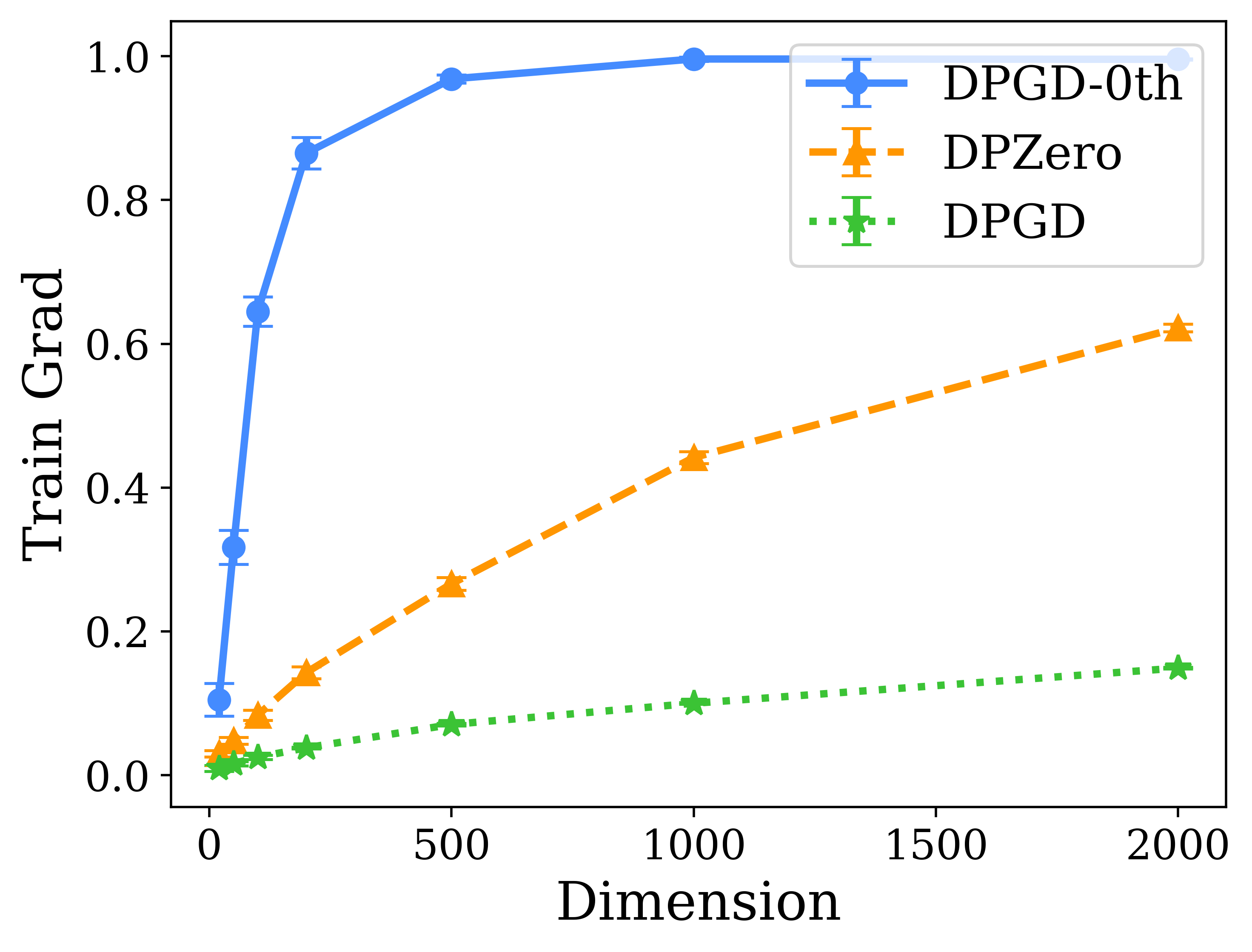
(a) $\,\text{Tr}(A)=\mathcal{O}(d)$.

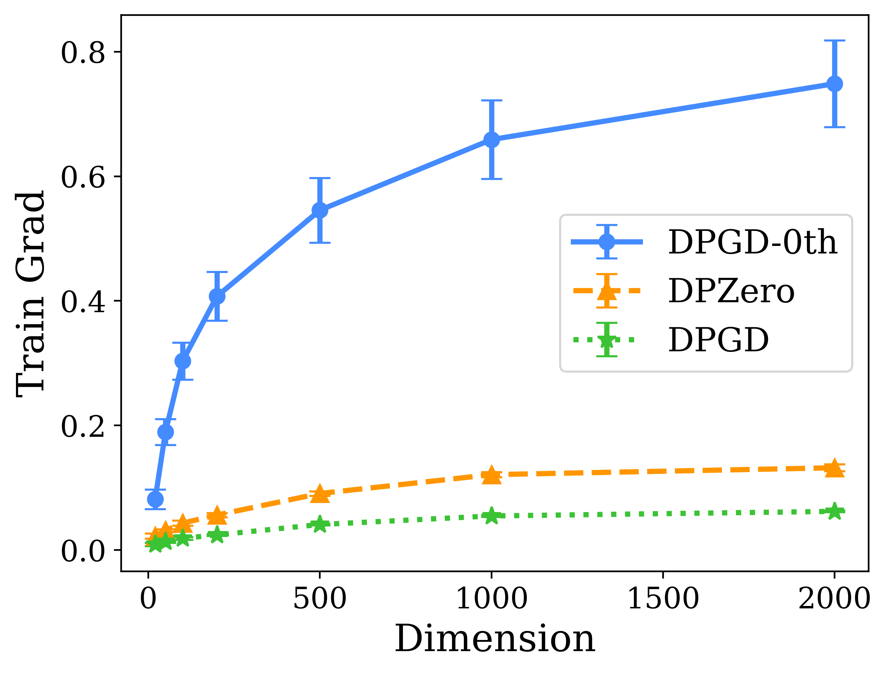
(b) $\,\text{Tr}(A)=\mathcal{O}(\sqrt{d})$.

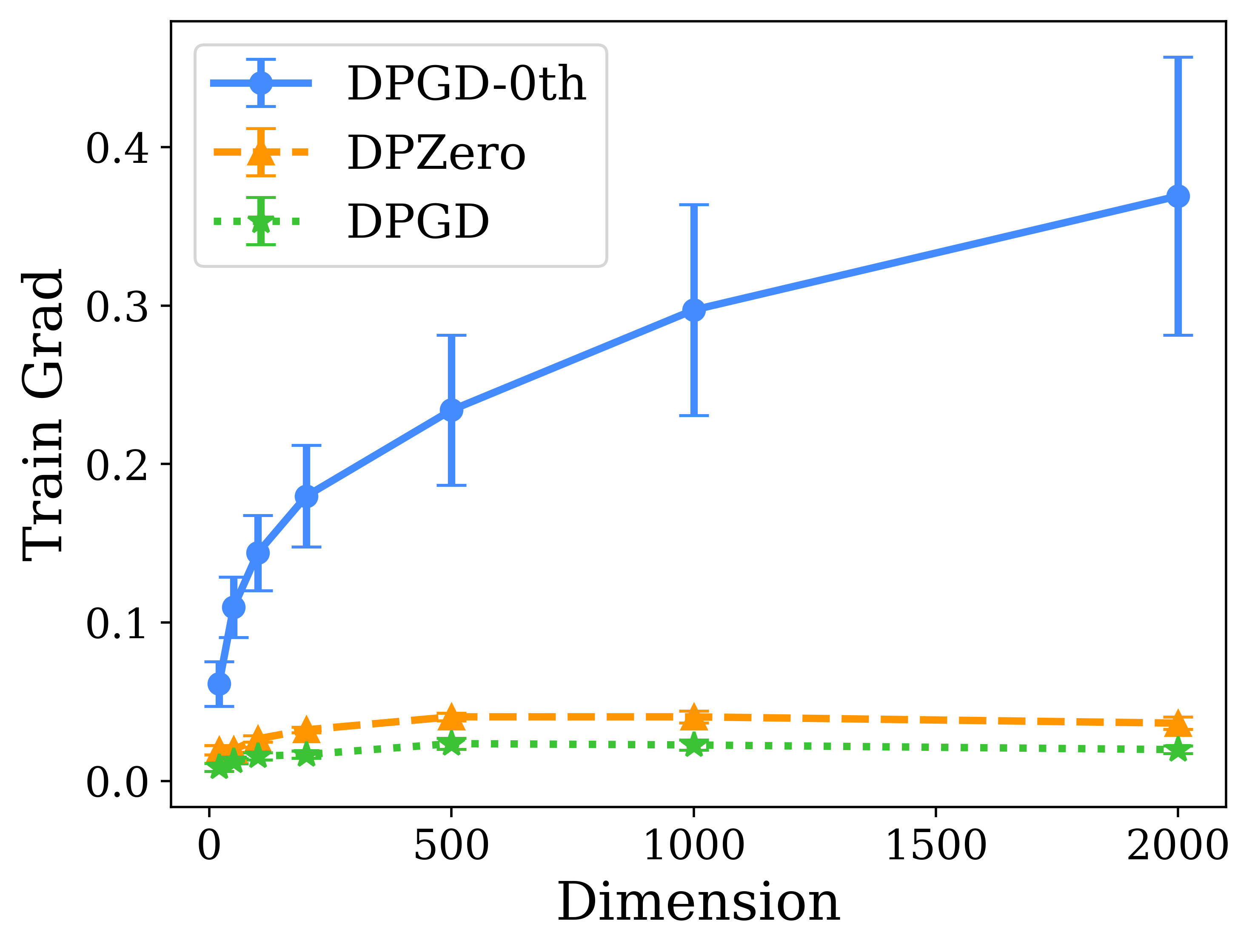
(c) $\,\text{Tr}(A)=\mathcal{O}(\log d)$.

Figure 2: Experiments on the quadratic loss with effective rank $\,\text{Tr}(A)$. For three different modes of the effective rank, we increase the problem dimension and report the best gradient norm evaluated on the training set.

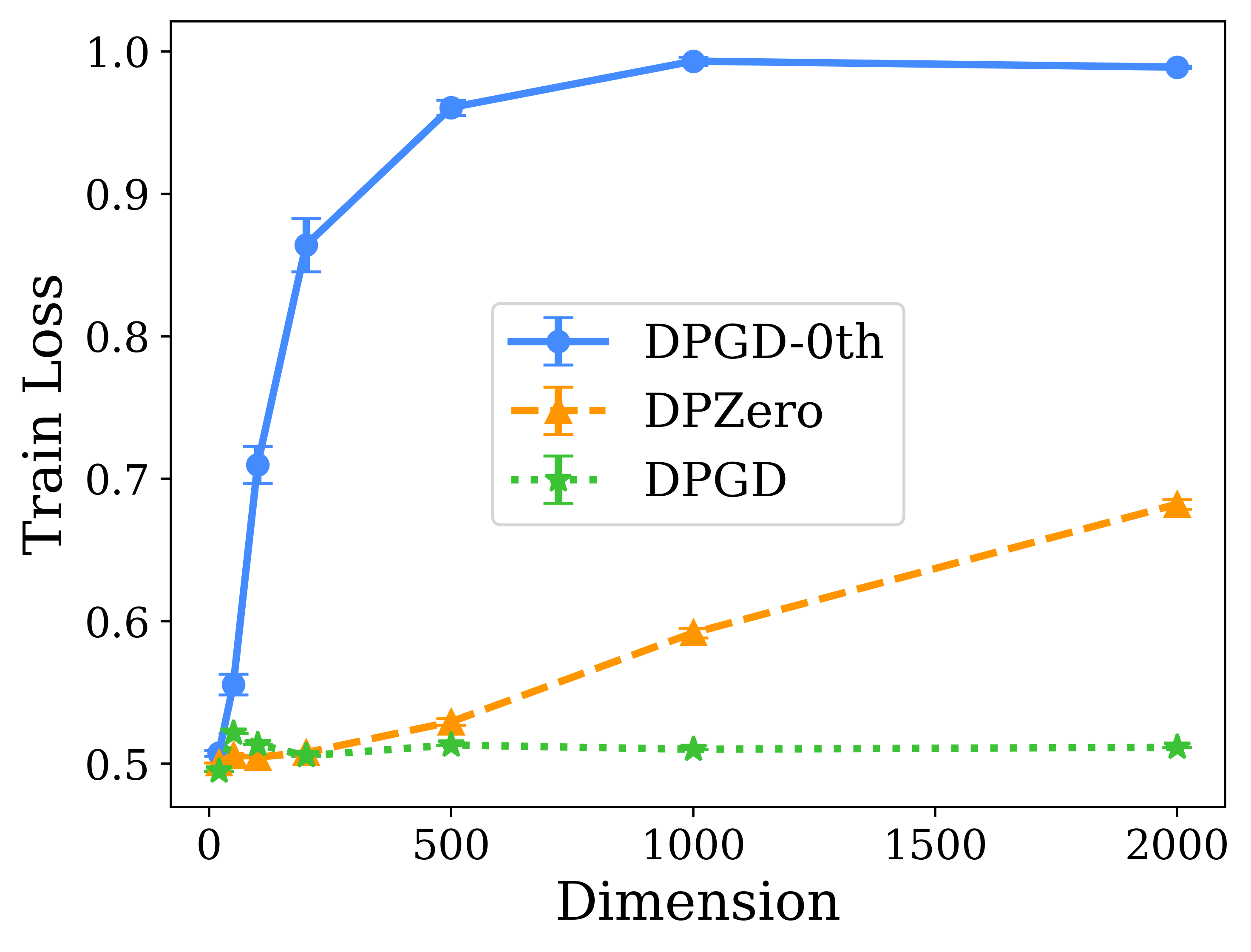
(a) $\,\text{Tr}(A)=\mathcal{O}(d)$.

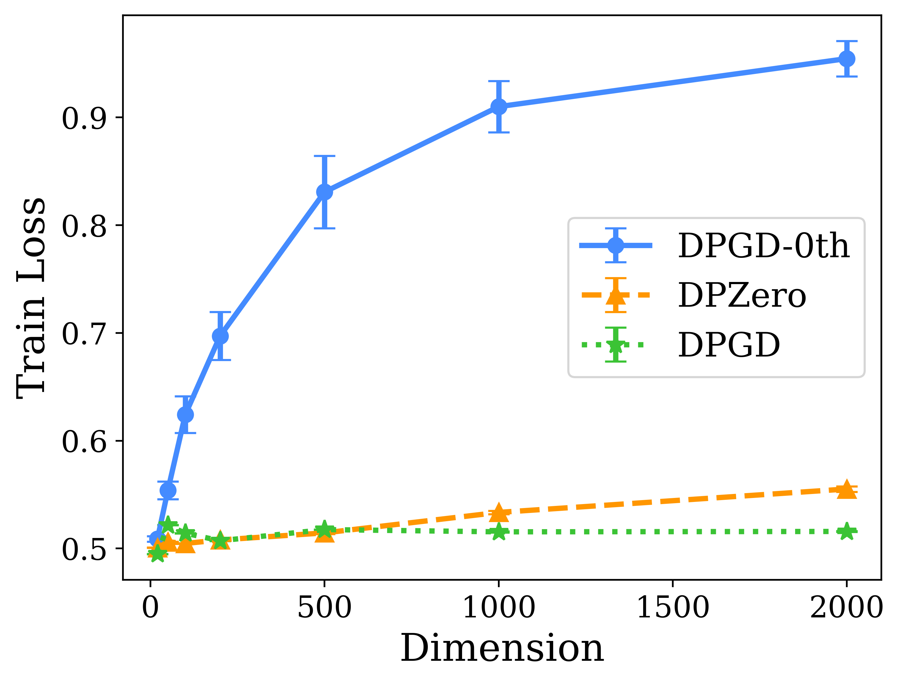
(b) $\,\text{Tr}(A)=\mathcal{O}(\sqrt{d})$.

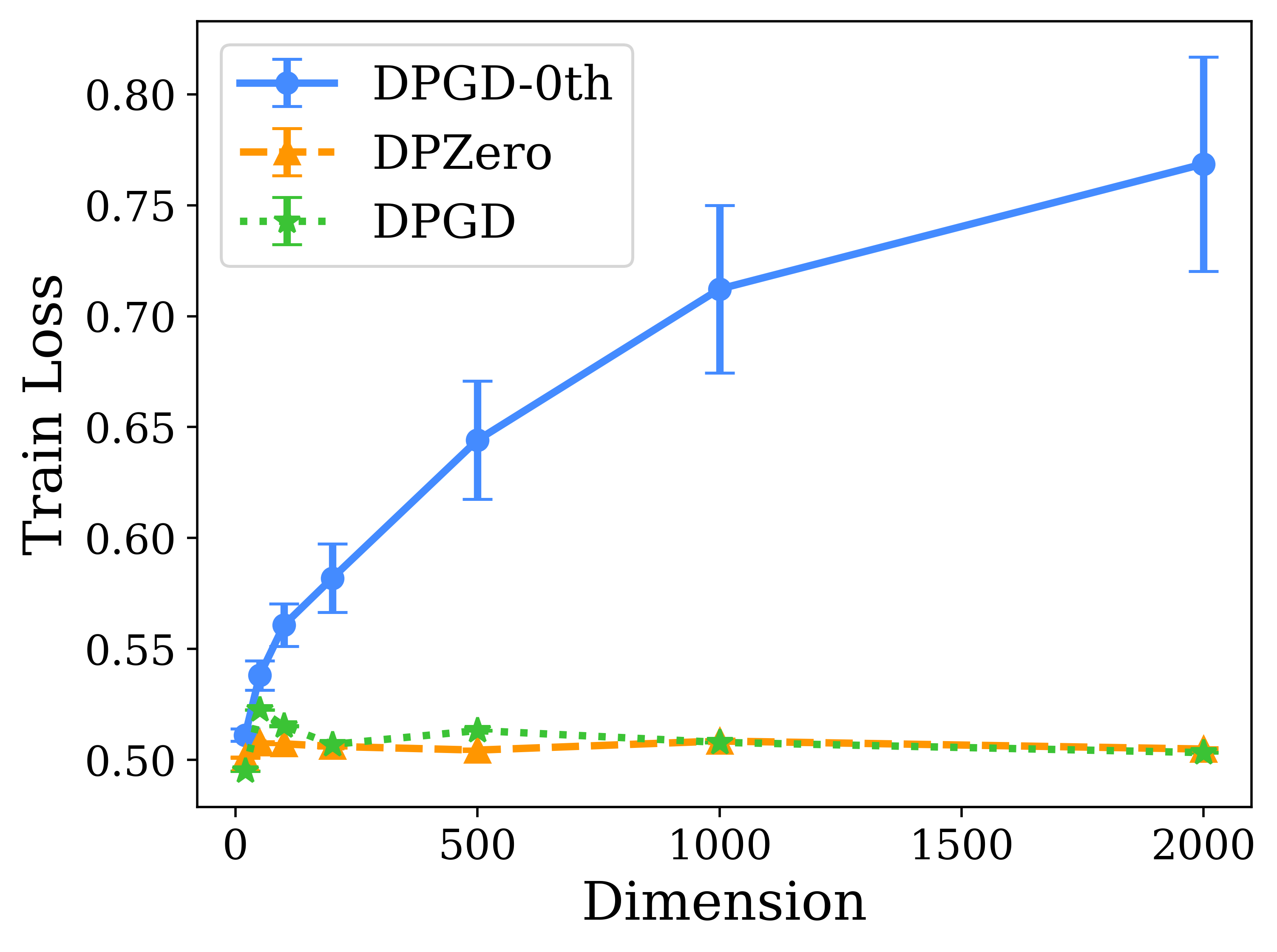
(c) $\,\text{Tr}(A)=\mathcal{O}(\log d)$.

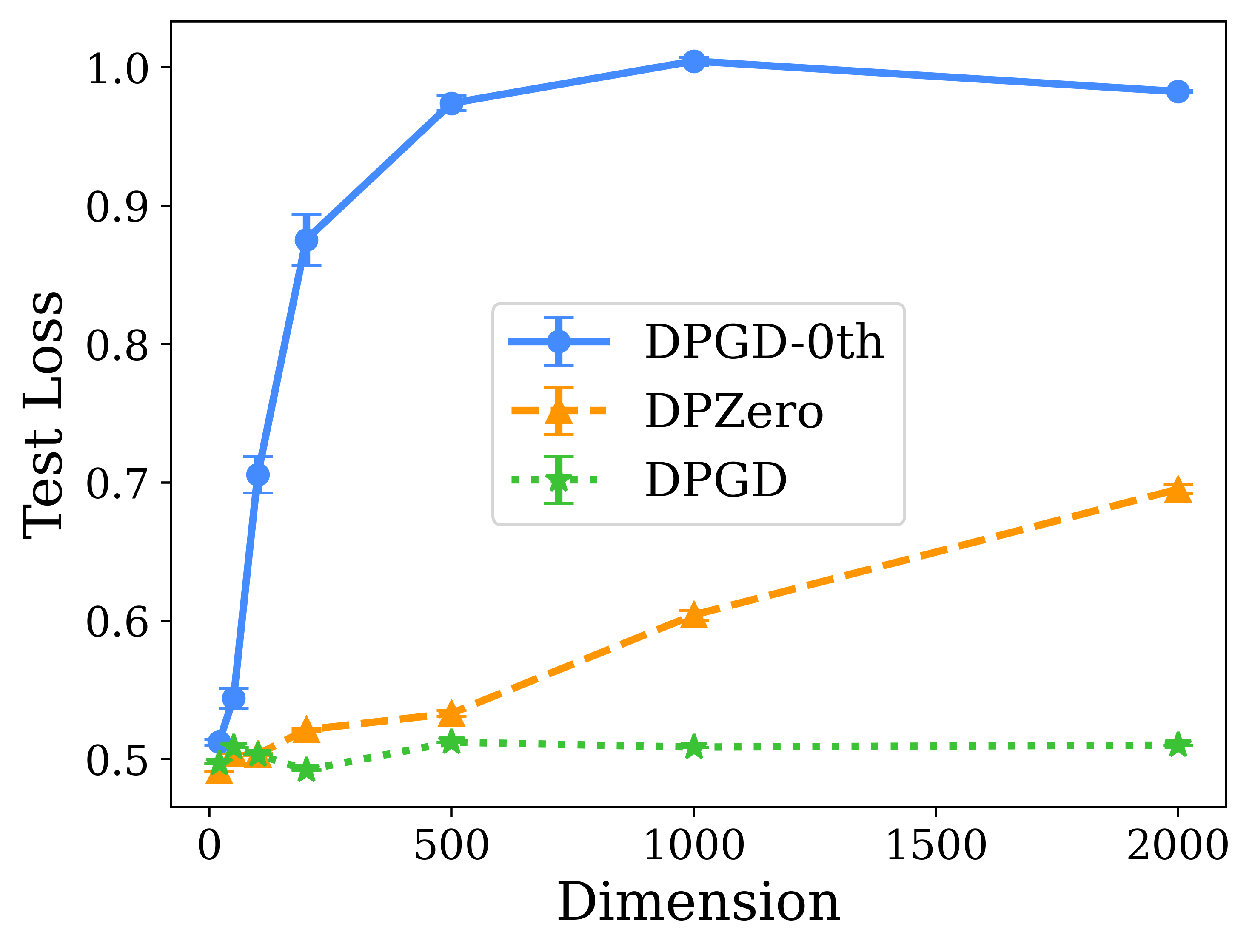
(d) $\,\text{Tr}(A)=\mathcal{O}(d)$.

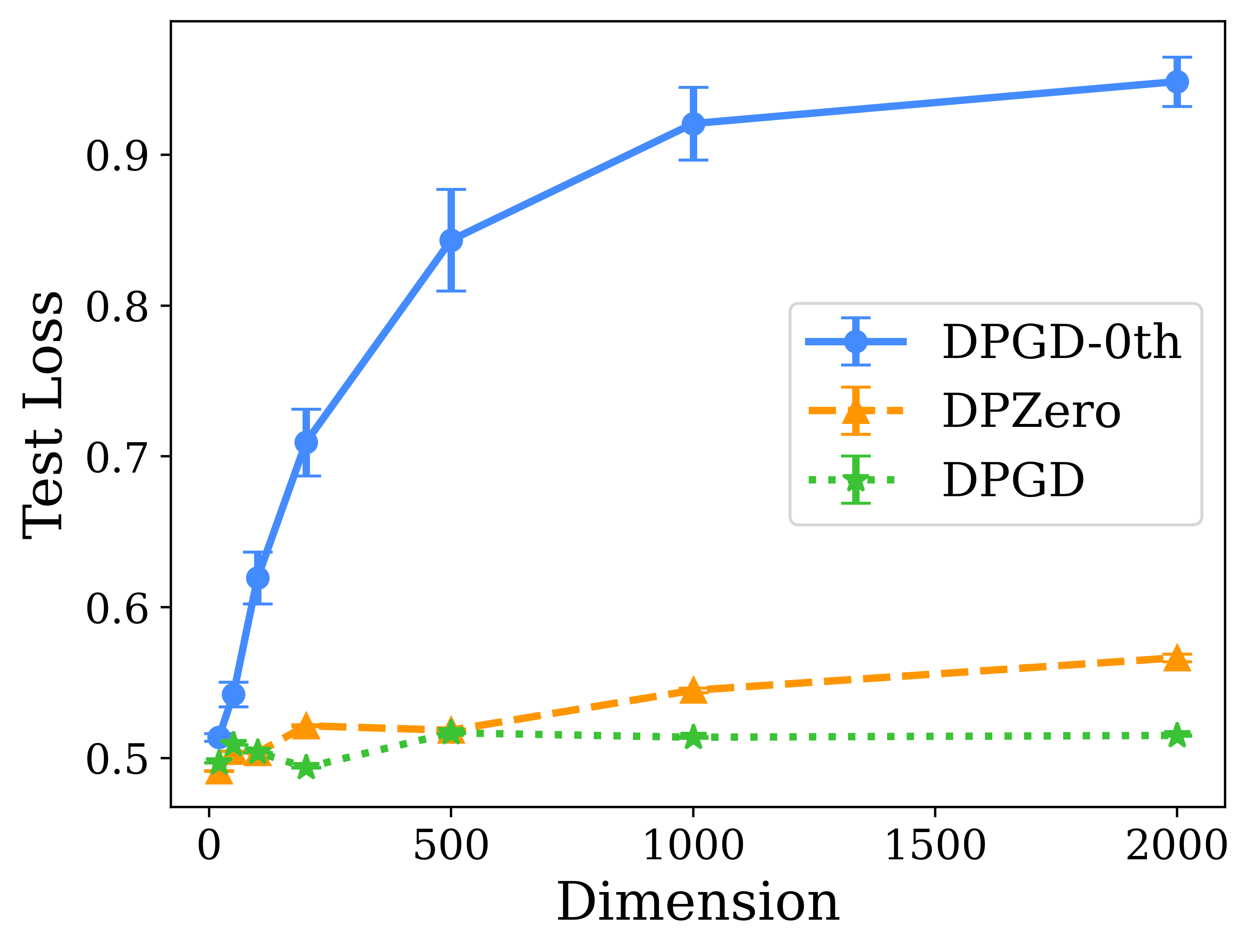
(e) $\,\text{Tr}(A)=\mathcal{O}(\sqrt{d})$.

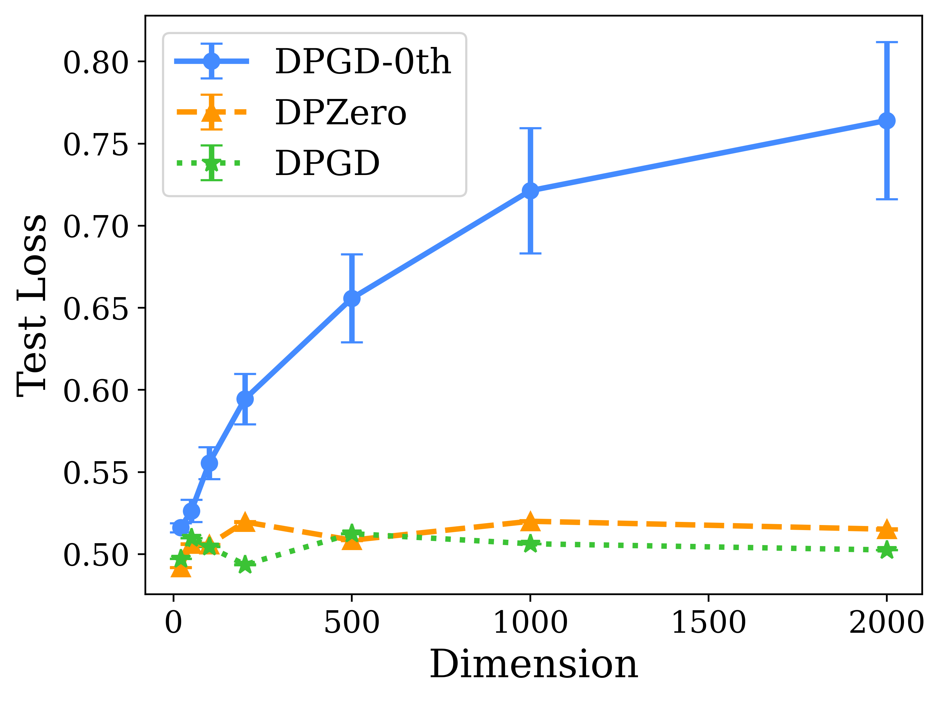
(f) $\,\text{Tr}(A)=\mathcal{O}(\log d)$.

Figure 3: Experiments on the quadratic loss with effective rank $\,\text{Tr}(A)$. For three different modes of the effective rank, we increase the problem dimension and report the best loss evaluated on both training set ((a), (b), and (c)) and test set ((d), (e), and (f)).

Since $\lVert A\rVert_{2}=1$ in all cases, the effective rank $r=\,\text{Tr}(A)$. For each mode of the effective rank, we increase the problem dimension $d$ from 20 to 2000. We perform a parameter search and plot the best gradient norm evaluated on the training set (see Figure 2) and a test set that follows the same distribution of the training set (see Figure 1). For completeness, we also plot both training and test loss in Figure 3. The key hyper-parameters used for the experiments are summarized in Table 4.

Table 4: Hyper-parameters used for the synthetic example on the quadratic loss. The number of iterations, stepsize, and clipping threshold are optimized through a grid search using given values. Other parameters are fixed to the listed values.

Hyper-parameters	Values
Number of training samples	10000
Number of test samples	10000
Dimension $d$	$\{20,50,100,200,500,1000,2000\}$
Privacy	$(\varepsilon=2,\delta=10^{-6})$
Smoothing $\lambda$ (DPZero and DPGD-0th)	$10^{-4}$
Number of iterations	$\{10,20,40,80,160,320,640,1280,2560,5120\}$
Stepsize	$\{10^{-5},3\times 10^{-5},10^{-4},3\times 10^{-4},0.001,0.003,0.01,0.03,0.1,0.3,1\}$
Clipping	$\{0.1,0.3,1,3,10,30,100,300\}$

In all figures, we observe that the performance of each method is improved with smaller effective rank. For each pattern of the effective rank, DPGD-0th (Algorithm 1) has the worst performance, while DP-GD consistently achieves the best results. When the effective rank is $d$, every method scales with the dimension. When the effective rank improves to $\log d$, DPZero and DP-GD become nearly dimension-independent, and DPZero matches the performance of the first-order method DP-GD. This validates our theoretical findings, as summarized in Table 1, and demonstrates the effectiveness of DPZero. We want to mention that a similar set of experiments to verify the performance of DP-GD when dimension increases was also provided by Li et al. [66]. Our implementation of this synthetic example is based on their code.

B.2 Private Fine-Tuning of the Language Model RoBERTa

We follow experiment settings in Malladi et al. [82] to evaluate the performance of DPZero in the private fine-tuning of RoBERTa [76] across six sentence classification datasets: SST-2 and SST-5 [106] for sentiment classification, SNLI [12], MNLI [125], and RTE [25, 50, 43, 11, 119] for natural language inference tasks, and TREC [117] for topic classification. In our experiments, we employ the same prompts as used in Malladi et al. [82], which are adapted from Gao et al. [40].

Implementation details.

Our implementation of DPZero utilizes the codebase provided by Malladi et al. [82]. For easier implementation and better memory efficiency, we follow Malladi et al. [82] to sample the zeroth-order direction $u_{t}$ from the Gaussian distribution $\mathcal{N}(0,\mathrm{I}_{d})$ instead of the sphere as stated in Algorithm 2. Table 5 compares the performance of DPZero on SST-2 and SST-5 when $u_{t}$ is sampled from Gaussian and sphere. Given the negligible differences between the two sampling strategies, we continue with the Gaussian sampling for its simplicity. Another strategy in the implementation to further save memory involves storing only the random seed for the generation of the zeroth-order direction $u_{t}$, rather than the complete vector, and regenerating this direction whenever it’s used. Although DPZero is stated for the full-batch case in Algorithm 2, we adopt a mini-batch setting in the experiments.

Table 5: Test accuracy (mean % $\pm$ standard error %) of DPZero when fine-tuning RoBERTa (355M) for SST-2 and SST-5 with $(\varepsilon=\{2,6\},\delta=10^{-5})$-DP and using different sampling strategies of the zeroth-order update direction $u_{t}$. No notable difference is observed when $u_{t}$ is sampled from either the Gaussian distribution or the Euclidean sphere.

Randomness	Gaussian		Sphere
	$\varepsilon=6$	$\varepsilon=2$	$\varepsilon=6$	$\varepsilon=2$
SST-2	$92.2\pm 0.3$	$91.8\pm 0.1$	$91.8\pm 0.1$	$91.5\pm 0.5$
SST-5	$49.3\pm 0.6$	$47.1\pm 0.9$	$49.9\pm 1.3$	$47.4\pm 1.3$

Hyper-parameter selection.

For all experiments, we employ a few-shot setting, utilizing 512 samples per class in the training set, randomly selected from the original dataset. The test set is also composed of 1000 randomly selected samples from the original test dataset. We fix the total number of iterations to be 10000, the batch size to be 64, and the smoothing parameter $\lambda=10^{-3}$ for both DPZero and the private zeroth-order baseline MeZO [82]. Note that the original results of MeZO reported in Malladi et al. [82] run for 100000 iterations. A parameter search of the learning rate for MeZO is performed, and it turns out $10^{-6}$ consistently yields the best performance. We then fix the learning rate to be $10^{-6}$ for DPZero and only search for the clipping threshold for different tasks. There is potential for improved performance by well-optimizing other hyper-parameters, such as the learning rate and the number of iterations. Regarding the first-order methods presented in Table 3, we set the number of iterations to be 1000, the clipping threshold to be 10, and the learning rate to be $10^{-5}$. All results are averaged through three different random seeds $\{42,13,21\}$ for selecting the few-shot datasets. The hyper-parameters used for our language model fine-tuning experiments are summarized in Table 6.

Table 6: Hyper-parameters used in DPZero for the language model fine-tuning tasks. We only optimize the clipping threshold through a grid search from 50 to 400. Other parameters are fixed to the listed values.

Hyper-parameters	Values
Number of training samples	512 per class
Number of test samples	1000
Number of iterations	10000
batch size	64
Privacy	$(\varepsilon=\{2,6\},\delta=10^{-5})$
Smoothing $\lambda$	$10^{-3}$
Stepsize	$10^{-6}$
Clipping	{50, 100, 150, 200, 250, 300, 400}

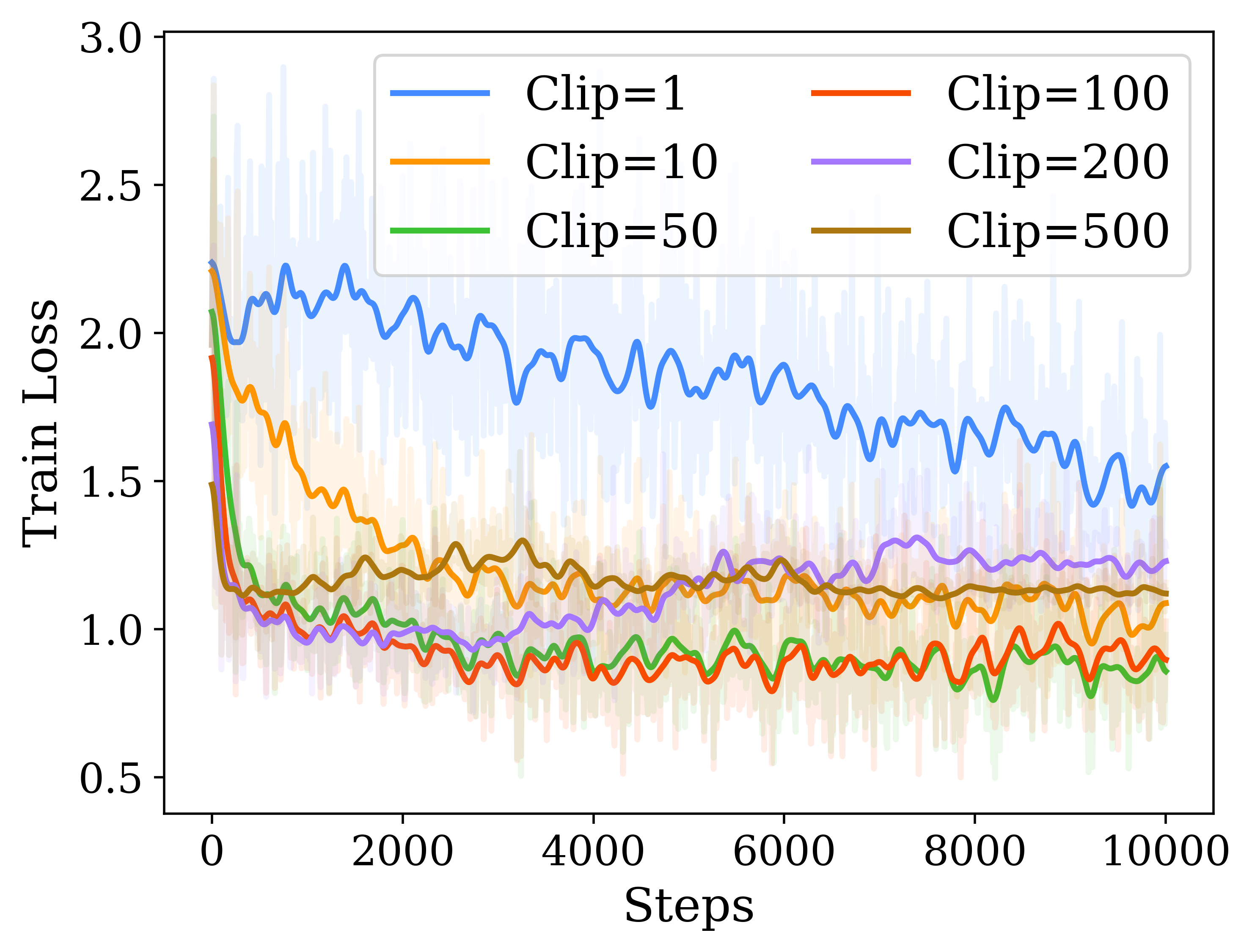
(a) Training Loss.

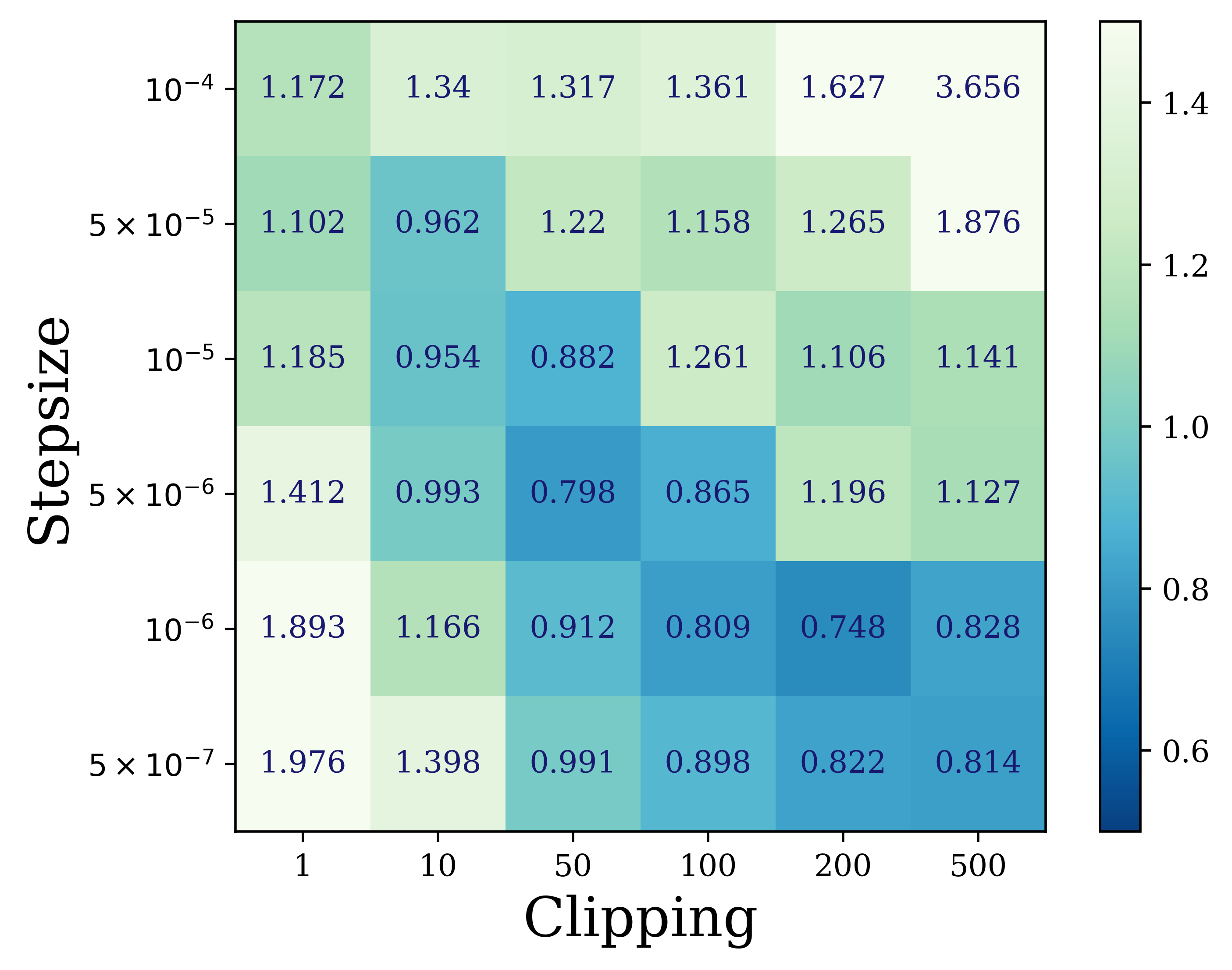
(b) Test Loss.

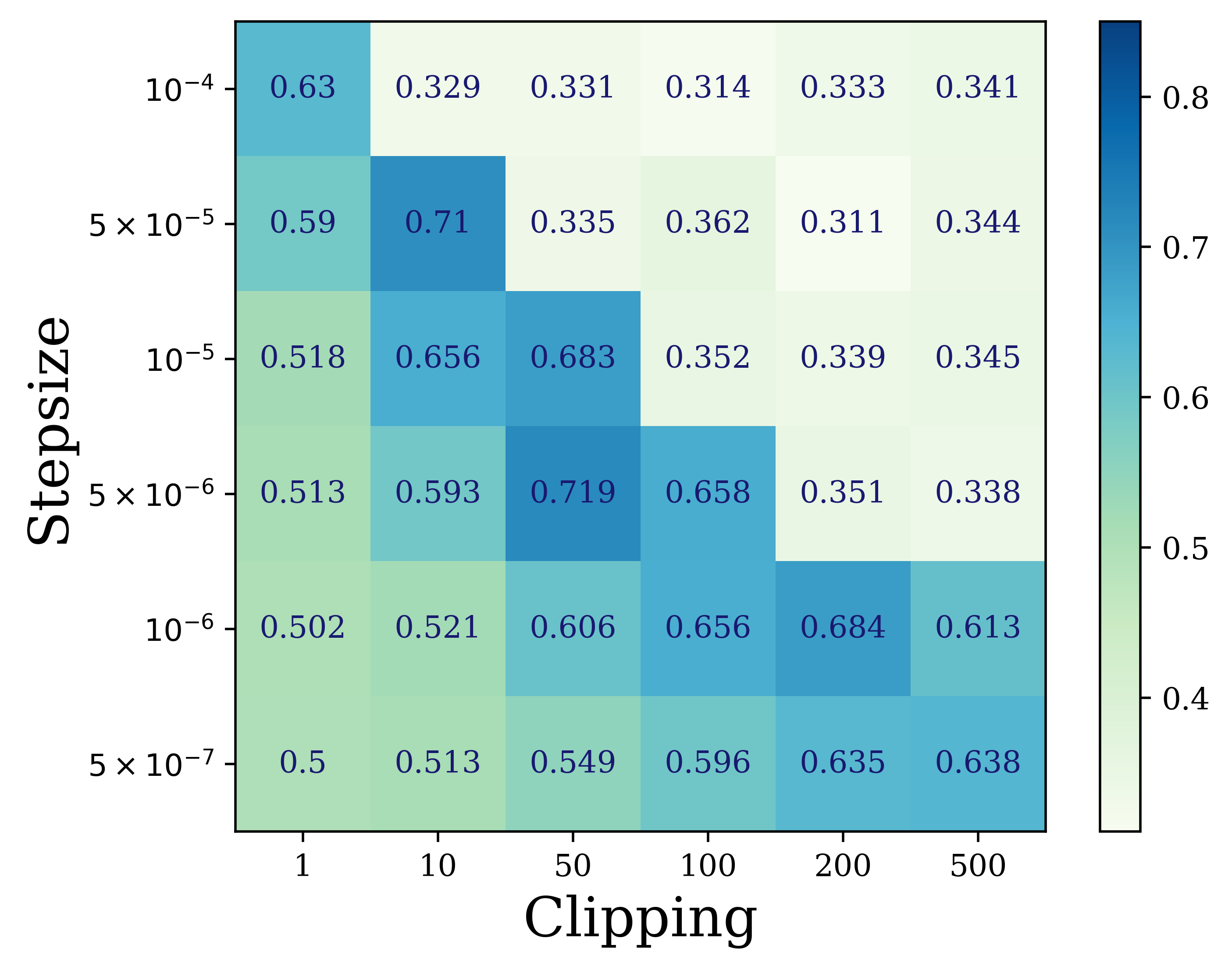
(c) Test Accuracy (%).

Figure 4: Experiments on private fine-tuning RoBERTa (125M) for SNLI with DPZero. (a) (Smoothed) training curves when fixing the stepsize to be $5\times 10^{-6}$ and varying the clipping threshold from 1 to 500. In the choice of clipping, a tradeoff emerges; larger clipping values result in unnecessarily high privacy noise, while smaller values can induce increased bias in the optimization process. (b) and (c) Test loss and accuracy (%) when varying the stepsize and clipping threshold together. Consistent with first-order methods [67], we observe that larger clipping necessitates smaller stepsizes, whereas smaller clipping favors larger stepsizes.

Clipping threshold.

Our findings indicate that the optimal clipping threshold for DPZero tends to be higher than that for first-order methods. This observation aligns with the theoretical outcomes presented in Theorem 3, where the clipping threshold for DPZero is $C=\mathcal{O}(L\sqrt{\log(nd)})$, in contrast to the $\mathcal{O}(L)$ threshold adequate for first-order methods. In the concurrent study by [110], the chosen clipping threshold is 0.05. However, their implementation applies the clipping to the term $f(x+\lambda u;\xi)-f(x-\lambda u;\xi)$. After normalization by $\lambda=10^{-3}$, it aligns with the order of magnitude used in our method. The validity of opting for a larger clipping threshold in DPZero is further confirmed through the private fine-tuning of RoBERTa (125M) on the SNLI dataset in Figure 4. An additional observation from our experiments is that the non-private baseline MeZO also appears to benefit from clipping. For instance, without clipping, the original MeZO encounters non-convergence issues at a stepsize of $5\times 10^{-6}$. Conversely, incorporating clipping permits the use of larger stepsizes and yields better results. A thorough investigation of this phenomenon is reserved for future research.

Appendix C Technical Lemmas

Lemma C.1.

Let $u$ be uniformly sampled from the Euclidean sphere $\sqrt{d}\cdot\mathbb{S}^{d-1}$, $a\in\mathbb{R}^{d}$ be some fixed vector independent of $u$, and $H\in\mathbb{R}^{d\times d}$ be some fixed matrix independent of $u$. We have that

• $\mathbb{E}[u]=0\,$ and $\,\mathbb{E}[uu^{\top}]=\mathrm{I}_{d}$.

• $\mathbb{E}_{u}[u^{\top}a]=0,\,\mathbb{E}_{u}[(u^{\top}a)^{2}]=\lVert a\rVert^{2}\,$ and $\forall\,C\geq 0$,

  $$\mathbb{P}(\lvert u^{\top}a\rvert\geq C)\leq 2\sqrt{2\pi}\exp\left(-\frac{C^{2}}{8\lVert a\rVert^{2}}\right).$$

• $\mathbb{E}_{u}[(u^{\top}a)u]=a\,$ and

  $$\mathbb{E}_{u}[(u^{\top}a)^{2}\lVert u\rVert^{2}]=d\lVert a\rVert^{2},$$

  $$\mathbb{E}_{u}[(u^{\top}a)^{2}uu^{\top}]=\frac{d}{d+2}\left(2aa^{\top}+\lVert a\rVert^{2}\mathrm{I}_{d}\right).$$

• $\mathbb{E}_{u}[u^{\top}Hu]=\emph{\,\text{Tr}}(H)\,$ and

  $$\mathbb{E}_{u}[(u^{\top}a)^{2}u^{\top}Hu]=\frac{d}{d+2}\left(2a^{\top}Ha+\lVert a\rVert^{2}\emph{\,\text{Tr}}(H)\right).$$

Proof.

$(i)$ is a standard result, e.g., in Duchi et al. [29], and follows by the symmetry of the sphere. For any $u\in\sqrt{d}\cdot\mathbb{S}^{d-1}$, it must be the case that $-u\in\sqrt{d}\cdot\mathbb{S}^{d-1}$ as well, which suggests that $\mathbb{E}[u]=0$. Since $\mathbb{E}[\sum_{i=1}^{d}u_{i}^{2}]=\mathbb{E}\lVert u\rVert^{2}=d$, we immediately have that $\mathbb{E}[u_{i}^{2}]=1$ for every $i$ by symmetry. Then for the off-diagonal terms, since for any $u=(u_{1},\cdots,u_{i},\cdots,u_{j},\cdots,u_{d})\in\sqrt{d}\cdot\mathbb{S}^{d-1}$, it must be the case that $(u_{1},\cdots,u_{i},\cdots,-u_{j},\cdots,u_{d})\in\sqrt{d}\cdot\mathbb{S}^{d-1}$ as well, which suggests that $\mathbb{E}[u_{i}u_{j}]=0$ when $i\neq j$. As a result, we can conclude that the matrix $\mathbb{E}[uu^{\top}]=\mathrm{I}_{d}$.

We then show $(ii)$. Applying $(i)$, we have that $\mathbb{E}_{u}[u^{\top}a]=0$, and that

$$\mathbb{E}_{u}[(u^{\top}a)^{2}] =\sum_{i=1}^{d}a_{i}^{2}\mathbb{E}[u_{i}^{2}]+\sum_{i\neq j}a_{i}a_{j}\mathbb{E}[u_{i}u_{j}]$$

$$=\lVert a\rVert^{2}.$$

The tail bound follows from Example 3.12 in Wainwright [118], where they show that for any function $h:\mathbb{S}^{d-1}\rightarrow\mathbb{R}$ such that $\forall x,y\in\mathbb{S}^{d-1}$,

$$\lvert h(x)-h(y)\rvert\leq\arccos(x^{\top}y),$$

when $x$ is uniformly sampled from $\mathbb{S}^{d-1}$, it holds that $\forall\,\gamma\geq 0$,

$$\mathbb{P}(\lvert h(x)-\mathbb{E}[h(x)]\rvert\geq\gamma)\leq 2\sqrt{2\pi}\exp\left(-\frac{d\gamma^{2}}{8}\right).$$ (8)

Let $h(x)=x^{\top}a/\lVert a\rVert$ for $x\in\mathbb{S}^{d-1}$. First, we have that $\forall x,y\in\mathbb{S}^{d-1}$,

$$\lvert h(x)-h(y)\rvert^{2} =\frac{\lvert(x-y)^{\top}a\rvert^{2}}{\lVert a\rVert^{2}}$$

$$\leq\lVert x-y\rVert^{2}$$

$$=2(1-x^{\top}y)$$

$$\leq(\arccos(x^{\top}y))^{2},$$

where we use the inequality that $\theta^{2}/2+\cos(\theta)-1\geq 0$ for $\theta\in[0,\pi]$ and let $x^{\top}y=\cos(\theta)$ such that $\arccos(x^{\top}y)=\theta$ for some $\theta\in[0,\pi]$. When $u$ is uniformly sampled from $\sqrt{d}\cdot\mathbb{S}^{d-1}$, we know $u/\sqrt{d}$ is uniformly from $\mathbb{S}^{d-1}$. Applying (8) for $h(x)=x^{\top}a/\lVert a\rVert$ where $x\in\mathbb{S}^{d-1}$, we obtain that

$$\mathbb{P}\left(\left\lvert\frac{u^{\top}a}{\sqrt{d}\lVert a\rVert}-\frac{\mathbb{E}[u^{\top}a]}{\sqrt{d}\lVert a\rVert}\right\rvert\geq\gamma\right)\leq 2\sqrt{2\pi}\exp\left(-\frac{d\gamma^{2}}{8}\right).$$

Setting $C=\gamma\sqrt{d}\lVert a\rVert$, the proof is complete since $\mathbb{E}[u^{\top}a]=0$. Similar results also exist in Theorem 5.1.4 of Vershynin [115], with all constants hidden behind some absolute $c$.

Next, we prove $(iii)$. Applying $(i)$, we have that

$$\mathbb{E}_{u}[(u^{\top}a)u_{i}] =a_{i}\mathbb{E}[u_{i}^{2}]+\sum_{j\neq i}a_{j}\mathbb{E}[u_{i}u_{j}]$$

$$=a_{i}.$$

This implies that $\mathbb{E}_{u}[(u^{\top}a)u]=a$. Applying $(ii)$, we obtain that

$$\mathbb{E}_{u}[(u^{\top}a)^{2}\lVert u\rVert^{2}] =d\cdot\mathbb{E}_{u}[(u^{\top}a)^{2}]$$

$$=d\lVert a\rVert^{2}.$$

For the expectation of the matrix, we start from the diagonal terms.

$$\begin{split}\mathbb{E}_{u}[(u^{\top}a)^{2}u_{i}^{2}]&=\sum_{j=1}^{d}a_{j}^{2}\mathbb{E}[u_{j}^{2}u_{i}^{2}]+\sum_{j\neq k}a_{j}a_{k}\mathbb{E}[u_{j}u_{k}u_{i}^{2}]\\ &=a_{i}^{2}\mathbb{E}[u_{i}^{4}]+\sum_{j\neq i}a_{j}^{2}\mathbb{E}[u_{j}^{2}u_{i}^{2}].\end{split}$$ (9)

Here, we use the property that $\mathbb{E}[u_{j}u_{k}u_{i}^{2}]=0$ for every $i$ when $j\neq k$. This follows from symmetry of the sphere such that for any $u=(u_{1},\cdots,u_{j},\cdots,u_{k},\cdots,u_{d})\in\sqrt{d}\cdot\mathbb{S}^{d-1}$, it must be the case that $(u_{1},\cdots,u_{j},\cdots,-u_{k},\cdots,u_{d})\in\sqrt{d}\cdot\mathbb{S}^{d-1}$ as well. Again by symmetry, we have that $\mathbb{E}[u_{i}^{4}]$ remains the same for every $i$, and $\mathbb{E}[u_{i}^{2}u_{j}^{2}]$ remains the same for every $i\neq j$. Denote $w_{1}=\mathbb{E}[u_{i}^{4}]$ and $w_{2}=\mathbb{E}[u_{i}^{2}u_{j}^{2}]$. Since it holds that

$$\sum_{i=1}^{d}\mathbb{E}_{u}[(u^{\top}a)^{2}u_{i}^{2}] =\mathbb{E}_{u}[(u^{\top}a)^{2}\lVert u\rVert^{2}]$$

$$=d\lVert a\rVert^{2},$$

taking summation over (9), we can have that

$$d\lVert a\rVert^{2} =\sum_{i=1}^{d}a_{i}^{2}\mathbb{E}[u_{i}^{4}]+\sum_{i=1}^{d}\sum_{j=1,j\neq i}^{d}a_{j}^{2}\mathbb{E}[u_{j}^{2}u_{i}^{2}]$$

$$=w_{1}\lVert a\rVert^{2}+w_{2}\sum_{i=1}^{d}(\lVert a\rVert^{2}-a_{i}^{2})$$

$$=w_{1}\lVert a\rVert^{2}+(d-1)w_{2}\lVert a\rVert^{2}.$$

This holds for arbitrary $a\in\mathbb{R}^{d}$, and thus we obtain that

$$w_{1}+(d-1)w_{2}=d.$$ (10)

We only compute $w_{1}=\mathbb{E}[u_{i}^{4}]$ by showing that $u_{i}^{2}/d$ actually follows the Beta distribution, and the value of $w_{2}$ can be derived from (10). First, $z/\lVert z\rVert$ is uniformly distributed on the unit sphere $\mathbb{S}^{d-1}$ for $z\in\mathbb{R}^{d}$ sampled from the standard multivariate Gaussian $\mathcal{N}(0,\mathrm{I}_{d})$ [87, 84]. This means that $z_{i}^{2}$ is distributed according to the $\chi^{2}$-distribution with 1 degree of freedom, and $\bar{z}_{i}^{2}:=\sum_{j\neq i}z_{j}^{2}$ is distributed according to the $\chi^{2}$-distribution with degree $(d-1)$. Since $\chi^{2}$-distribution is a special case of the Gamma distribution and $z_{i}^{2}$, $\bar{z}_{i}^{2}$ are independent, we conclude [24, 48] that $z_{i}^{2}/(z_{i}^{2}+\bar{z}_{i}^{2})$ has the Beta distribution with parameters $1/2$ and $(d-1)/2$. Finally, since $u/\sqrt{d}$ is uniformly distributed on $\mathbb{S}^{d-1}$, by symmetry of the sphere, we know that $u_{i}^{2}/d$ has the same Beta distribution as $z_{i}^{2}/(z_{i}^{2}+\bar{z}_{i}^{2})$. The mean and variance of Beta$(1/2,(d-1)/2)$ is $1/d$ and $2(d-1)/(d^{2}(d+2))$. This suggests that $\mathbb{E}[u_{i}^{2}]=1$, as already proved in $(i)$, and that

$$w_{1} =\mathbb{E}[(u_{i}^{2}-\mathbb{E}[u_{i}^{2}])^{2}]+(\mathbb{E}[u_{i}^{2}])^{2}$$

$$=d^{2}\left(\frac{2(d-1)}{d^{2}(d+2)}+\frac{1}{d^{2}}\right)$$

$$=\frac{3d}{d+2}.$$

By (10), we know $w_{2}=d/(d+2)$. According to (9), we have that the diagonal terms

$$\mathbb{E}_{u}[(u^{\top}a)^{2}u_{i}^{2}] =w_{1}a_{i}^{2}+w_{2}(\lVert a\rVert^{2}-a_{i}^{2})$$

$$=\frac{2d}{d+2}a_{i}^{2}+\frac{d}{d+2}\lVert a\rVert^{2}.$$

Then we compute the off-diagonal entries for $i\neq j$. By the same reasoning as (9), we have that

$$\mathbb{E}_{u}[(u^{\top}a)^{2}u_{i}u_{j}] =\sum_{i\neq j}a_{i}a_{j}\mathbb{E}[u_{i}^{2}u_{j}^{2}]$$

$$=\frac{2d}{d+2}a_{i}a_{j}.$$

All other terms equal to 0 by symmetry of the sphere. Combining both diagonal and off-diagonal elements, we have that $\mathbb{E}_{u}[(u^{\top}a)^{2}uu^{\top}]=(d/(d+2))(2aa^{\top}+\lVert a\rVert^{2}\mathrm{I}_{d})$. Similar results are also shown in Appendix F of Malladi et al. [82].

Finally, we give the proof of $(iv)$. For the first statement, applying $(i)$ in this lemma, we have that

$$\mathbb{E}_{u}\left[u^{\top}Hu\right] =\mathbb{E}\Big{[}\,\text{Tr}(uu^{\top}H)\Big{]}$$

$$=\,\text{Tr}\Big{(}\mathbb{E}[uu^{\top}]\cdot H\Big{)}$$

$$=\,\text{Tr}(H).$$

Similarly for the second statement, we apply $(iii)$ in this lemma and obtain that

$$\mathbb{E}_{u}\left[(u^{\top}a)^{2}u^{\top}Hu\right] =\mathbb{E}\Big{[}(u^{\top}a)^{2}\cdot\,\text{Tr}(uu^{\top}H)\Big{]}$$

$$=\mathbb{E}\Big{[}\,\text{Tr}\Big{(}(u^{\top}a)^{2}uu^{\top}\cdot H\Big{)}\Big{]}$$

$$=\,\text{Tr}\Big{(}\mathbb{E}\Big{[}(u^{\top}a)^{2}uu^{\top}\Big{]}\cdot H\Big{)}$$

$$=\frac{2d}{d+2}\,\text{Tr}(aa^{\top}H)+\frac{d}{d+2}\lVert a\rVert^{2}\,\text{Tr}(H)$$

$$=\frac{2d}{d+2}a^{\top}Ha+\frac{d}{d+2}\lVert a\rVert^{2}\,\text{Tr}(H).$$

This concludes the proof. ∎

Lemma C.2.

Let $u$ be uniformly sampled from the Euclidean sphere $\sqrt{d}\,\mathbb{S}^{d-1}$ and $v$ be uniformly sampled from the Euclidean ball $\sqrt{d}\,\mathbb{B}^{d}=\{x\in\mathbb{R}^{d}\,|\,\lVert x\rVert\leq\sqrt{d}\}$. For any function $f(x):\mathbb{R}^{d}\rightarrow\mathbb{R}$ and $\lambda>0$, we define its zeroth-order gradient estimator as $g_{\lambda}(x)=((f(x+\lambda u)-f(x-\lambda u))/(2\lambda))u$, and the smoothed function $f_{\lambda}(x)=\mathbb{E}_{v}[f(x+\lambda v)]$. The following properties hold:

• $f_{\lambda}(x)$ is differentiable and $\mathbb{E}_{u}[g_{\lambda}(x)]=\nabla f_{\lambda}(x)$.

• If $f(x)$ is $\ell$-smooth, then we have that

  $$\lVert\nabla f(x)-\nabla f_{\lambda}(x)\rVert \leq \frac{\ell}{2}\lambda d^{3/2},$$

  $$\mathbb{E}_{u}[\,\lVert g_{\lambda}(x)\rVert^{2}\,] \leq 2d\cdot\lVert\nabla f(x)\rVert^{2}+\frac{\ell^{2}}{2}\lambda^{2}d^{3}.$$

The above results are consistent with $(iii)$ in Lemma C.1 when $\lambda\to 0$ and $f(x)$ is differentiable such that the two-point estimator reduces to the directional derivative $g_{0}(x)=u^{\top}\nabla f(x)u$.

Proof.

We first show $(i)$. Similarly to Lemma 10 in Shamir [101], we have that

$$\mathbb{E}_{u\in\sqrt{d}\cdot\mathbb{S}^{d-1}}[g_{\lambda}(x)]=\mathbb{E}_{u\in\sqrt{d}\cdot\mathbb{S}^{d-1}}\left[\frac{f(x+\lambda u)u}{\lambda}\right].$$

Applying Lemma 2.1 in Flaxman et al. [36], we know

$$\mathbb{E}_{u^{\prime}\in\mathbb{S}^{d-1}}[f(x+\lambda^{\prime}u^{\prime})u^{\prime}]=\frac{\lambda^{\prime}}{d}\nabla\mathbb{E}_{v^{\prime}\in\mathbb{B}^{d}}[f(x+\lambda^{\prime}v^{\prime})].$$

Introducing $u=\sqrt{d}u^{\prime}$, $v=\sqrt{d}v^{\prime}$ and $\lambda=\lambda^{\prime}/\sqrt{d}$, we thus obtain

$$\mathbb{E}_{u\in\sqrt{d}\cdot\mathbb{S}^{d-1}}\left[\frac{f(x+\lambda u)u}{\lambda}\right] =\mathbb{E}_{u^{\prime}\in\mathbb{S}^{d-1}}\left[\frac{f(x+\lambda^{\prime}u^{\prime})u^{\prime}d}{\lambda^{\prime}}\right]$$

$$=\nabla\mathbb{E}_{v^{\prime}\in\mathbb{B}^{d}}[f(x+\lambda^{\prime}v^{\prime})]$$

$$=\nabla\mathbb{E}_{v\in\sqrt{d}\cdot\mathbb{B}^{d}}[f(x+\lambda v)].$$

The proof of $(ii)$ mostly follows from Nesterov and Spokoiny [89], where the results are originally obtained for the case that $u$ is sampled from the standard multivariate Gaussian distribution. By $(iii)$ in Lemma C.1 and $(i)$ here, we have that for $u$ uniformly sampled from $\sqrt{d}\cdot\mathbb{S}^{d-1}$,

$$\lVert\nabla f(x)-\nabla f_{\lambda}(x)\rVert =\left\lVert\mathbb{E}_{u}[(u^{\top}\nabla f(x))u]-\mathbb{E}_{u}\left[\frac{f(x+\lambda u)-f(x-\lambda u)}{2\lambda}u\right]\right\rVert$$

$$\leq\mathbb{E}_{u}\left\lVert\left(\frac{f(x+\lambda u)-f(x-\lambda u)}{2\lambda}-u^{\top}\nabla f(x)\right)u\right\rVert$$

$$\leq\frac{\sqrt{d}}{2\lambda}\mathbb{E}_{u}\lvert f(x+\lambda u)-f(x)-\lambda u^{\top}\nabla f(x)\rvert$$

$$\quad+\frac{\sqrt{d}}{2\lambda}\mathbb{E}_{u}\lvert f(x)-f(x-\lambda u)-\lambda u^{\top}\nabla f(x)\rvert$$

$$\leq\frac{\ell}{2}\lambda d^{3/2},$$

where in the last step we use smoothness of $f(x)$ such that $\lvert f(x+\lambda u)-f(x)-\lambda u^{\top}\nabla f(x)\rvert\leq\ell\lambda^{2}d/2$ and the same holds for $\lvert f(x)-f(x-\lambda u)-\lambda u^{\top}\nabla f(x)\rvert=\lvert f(x-\lambda u)-f(x)+\lambda u^{\top}\nabla f(x)\rvert$. The last statement holds similarly:

$$\mathbb{E}_{u}[\lVert g_{\lambda}(x)\rVert^{2}] =\frac{d}{4\lambda^{2}}\mathbb{E}_{u}[(f(x+\lambda u)-f(x-\lambda u))^{2}]$$

$$\leq 2d\cdot\mathbb{E}_{u}[(u^{\top}\nabla f(x))^{2}]+\frac{d}{2\lambda^{2}}\mathbb{E}_{u}[(f(x+\lambda u)-f(x-\lambda u)-2\lambda u^{\top}\nabla f(x))^{2}]$$

$$\leq 2d\cdot\mathbb{E}_{u}[(u^{\top}\nabla f(x))^{2}]+\frac{d}{\lambda^{2}}\mathbb{E}_{u}[(f(x+\lambda u)-f(x)-\lambda u^{\top}\nabla f(x))^{2}]$$

$$\quad+\frac{d}{\lambda^{2}}\mathbb{E}_{u}[(f(x)-f(x-\lambda u)-\lambda u^{\top}\nabla f(x))^{2}]$$

$$\leq 2d\cdot\lVert\nabla f(x)\rVert^{2}+\frac{\ell^{2}}{2}\lambda^{2}d^{3},$$ (11)

where in the last step we use Lemma C.1 and smoothness of $f(x)$. ∎

Appendix D Detailed Proof and Analysis of DPGD-0th (Algorithm 1)

Proof of Theorem 1.

The privacy guarantees directly follow from Lemma 2.2 noticing that the sensitivity is $2C/n$. Note that the original advanced composition theorem in Kairouz et al. [58] is stated for the case where the output of $\mathcal{A}$ is a scalar. Given the spherical symmetry properties of Gaussian noise, the results can be readily extended to multiple dimensions, as outlined in Lemma 1 of Kenthapadi et al. [61] where the basis can be selected in a way such that $\mathcal{A}(S)$ and $\mathcal{A}(S^{\prime})$ differ in exactly one dimension.

We then focus on the utility guarantee on $\mathbb{E}[\lVert\nabla F_{S}(x_{\tau})\rVert^{2}]$. Since $f(x;\xi)$ is $L$-Lipschitz for every $\xi$ by Assumption 3.1 and $\lVert u_{t}\rVert=\sqrt{d}$ by its construction, we have that

$$\lVert g_{\lambda}(x_{t};\xi_{i})\rVert =\frac{\lvert f(x_{t}+\lambda u_{t};\xi_{i})-f(x_{t}-\lambda u_{t};\xi_{i})\rvert}{2\lambda}\lVert u_{t}\rVert$$

$$\leq L\lVert u_{t}\rVert^{2}$$

$$=Ld.$$

This means $\,\text{clip}_{C}(g_{\lambda}(x_{t};\xi_{i}))=g_{\lambda}(x_{t};\xi_{i})$ when setting $C=Ld$. For notation simplicity, we let

$$G_{\lambda}(x_{t}) :=\frac{1}{n}\sum_{i=1}^{n}g_{\lambda}(x_{t};\xi_{i})$$

$$=\frac{1}{n}\sum_{i=1}^{n}\frac{f(x_{t}+\lambda u_{t};\xi_{i})-f(x_{t}-\lambda u_{t};\xi_{i})}{2\lambda}u_{t}$$

$$=\frac{F_{S}(x_{t}+\lambda u_{t})-F_{S}(x_{t}-\lambda u_{t})}{2\lambda}u_{t}.$$

Algorithm 1 reduces to $x_{t+1}=x_{t}-\alpha(G_{\lambda}(x_{t})+z_{t})$. By smoothness of $F_{S}(x)$, we have that

$$F_{S}(x_{t+1}) \leq F_{S}(x_{t})+\nabla F_{S}(x_{t})^{\top}(x_{t+1}-x_{t})+\frac{\ell}{2}\lVert x_{t+1}-x_{t}\rVert^{2}$$

$$=F_{S}(x_{t})-\alpha\nabla F_{S}(x_{t})^{\top}(G_{\lambda}(x_{t})+z_{t})+\frac{\ell}{2}\alpha^{2}\lVert G_{\lambda}(x_{t})\rVert^{2}+\frac{\ell}{2}\alpha^{2}\lVert z_{t}\rVert^{2}+\ell\alpha^{2}z_{t}^{\top}G_{\lambda}(x_{t}).$$

Since $z_{t}$ is sampled from $\mathcal{N}(0,\sigma^{2}\mathrm{I}_{d})$ and is independent of $x_{t}$, $u_{t}$ and $S$, we have that

$$\mathbb{E}_{z_{t}}[F_{S}(x_{t+1})]\leq F_{S}(x_{t})-\alpha\nabla F_{S}(x_{t})^{\top}G_{\lambda}(x_{t})+\frac{\ell}{2}\alpha^{2}\lVert G_{\lambda}(x_{t})\rVert^{2}+\frac{\ell}{2}\alpha^{2}\,d\,\sigma^{2}.$$

Define $F_{\lambda}(x):=\mathbb{E}_{v}[F_{S}(x+\lambda v)]$ for $v$ sampled uniformly from the Euclidean ball $\sqrt{d}\cdot\mathbb{B}^{d}$. By Lemma C.2, we know $\mathbb{E}_{u_{t}}[G_{\lambda}(x_{t})]=\nabla F_{\lambda}(x_{t})$. Since $u_{t}$ is independent of $x_{t}$ and $S$, taking expectation with respect to $u_{t}$ and applying $(ii)$ in Lemma C.2, we obtain that

$$\mathbb{E}_{z_{t},u_{t}}[F_{S}(x_{t+1})] \leq F_{S}(x_{t})-\alpha\nabla F_{S}(x_{t})^{\top}\nabla F_{\lambda}(x_{t})+\frac{\ell}{2}\alpha^{2}\mathbb{E}_{u_{t}}[\lVert G_{\lambda}(x_{t})\rVert^{2}]+\frac{\ell}{2}\alpha^{2}\,d\,\sigma^{2}$$

$$=F_{S}(x_{t})-\frac{\alpha}{2}\lVert\nabla F_{S}(x_{t})\rVert^{2}-\frac{\alpha}{2}\lVert\nabla F_{\lambda}(x_{t})\rVert^{2}+\frac{\alpha}{2}\lVert\nabla F_{\lambda}(x_{t})-\nabla F_{S}(x_{t})\rVert^{2}$$

$$\quad+\frac{\ell}{2}\alpha^{2}\,\mathbb{E}_{u_{t}}[\lVert G_{\lambda}(x_{t})\rVert^{2}]+\frac{\ell}{2}\alpha^{2}\,d\,\sigma^{2}$$

$$\leq F_{S}(x_{t})-\frac{\alpha}{2}(1-2d\ell\alpha)\lVert\nabla F_{S}(x_{t})\rVert^{2}+\frac{\ell^{2}}{8}\alpha(1+2\ell\alpha)\lambda^{2}d^{3}+\frac{\ell}{2}\alpha^{2}\,d\,\sigma^{2}.$$ (12)

Choosing $\alpha=1/(4\ell d)$ such that $1-2d\ell\alpha=1/2$ and $2\ell\alpha<1$, we obtain that

$$\mathbb{E}[\lVert\nabla F_{S}(x_{t})\rVert^{2}] <\frac{4\,\mathbb{E}[F_{S}(x_{t})-F_{S}(x_{t+1})]}{\alpha}+\ell^{2}\lambda^{2}d^{3}+2\ell\alpha\,d\sigma^{2}$$

$$=\frac{4\,\mathbb{E}[F_{S}(x_{t})-F_{S}(x_{t+1})]}{\alpha}+\ell^{2}\lambda^{2}d^{3}+\frac{64\ell C^{2}\,\alpha T\,d\log(e+(\varepsilon/\delta))}{n^{2}\varepsilon^{2}}$$

$$=\frac{4\,\mathbb{E}[F_{S}(x_{t})-F_{S}(x_{t+1})]}{\alpha}+\ell^{2}\lambda^{2}d^{3}+\frac{64\ell L^{2}\,\alpha T\,d^{3}\log(e+(\varepsilon/\delta))}{n^{2}\varepsilon^{2}}.$$

As a result, taking summation from $t=0$ to $T-1$ and dividing both sides by $T$, we have that

$$\mathbb{E}[\lVert\nabla F_{S}(x_{\tau})\rVert^{2}] =\frac{1}{T}\sum_{t=0}^{T-1}\mathbb{E}[\lVert\nabla F_{S}(x_{t})\rVert^{2}]$$

$$\leq\frac{4(F_{S}(x_{0})-F_{S}^{*})}{\alpha T}+\ell^{2}\lambda^{2}d^{3}+\frac{64\ell L^{2}\,\alpha T\,d^{3}\log(e+(\varepsilon/\delta))}{n^{2}\varepsilon^{2}}$$

$$\leq\frac{16(\ell(F_{S}(x_{0})-F_{S}^{*})+2L^{2})d\sqrt{d\log(e+(\varepsilon/\delta))}}{n\varepsilon},$$

with the choice of parameters

$$\alpha T=\frac{n\varepsilon}{4\ell d\sqrt{d\log(e+(\varepsilon/\delta))}},\quad\lambda\leq\frac{4L}{\ell d}\left(\frac{\sqrt{d\log(e+(\varepsilon/\delta))}}{n\varepsilon}\right)^{1/2}.$$

This suggests that the total number of iteration is $T=n\varepsilon/\sqrt{d\log(e+(\varepsilon/\delta))}$ and the total number of zeroth-order gradient computations is $nT=n^{2}\varepsilon/\sqrt{d\log(e+(\varepsilon/\delta))}$. Note that the above selection of parameters ensures scale invariance. ∎

Proof of Theorem 2.

The privacy analysis remains the same as before, and we focus on the utility analysis on $\mathbb{E}\lVert\nabla F_{S}(x_{\tau})\rVert^{2}$. By the same reasoning, when setting $C=Ld$, Algorithm 1 reduces to $x_{t+1}=x_{t}-\alpha(G_{\lambda}(x_{t})+z_{t})$ where $G_{\lambda}(x_{t})=(F_{S}(x_{t}+\lambda u_{t})-F_{S}(x_{t}-\lambda u_{t}))u_{t}/(2\lambda)$. By Taylor’s theorem with remainder, for some $\theta\in(0,1)$, we have that

$$F_{S}(x_{t+1}) =F_{S}(x_{t})+\nabla F_{S}(x_{t})^{\top}(x_{t+1}-x_{t})+\frac{1}{2}(x_{t+1}-x_{t})^{\top}\nabla^{2}F_{S}(x_{t}+\theta(x_{t+1}-x_{t}))(x_{t+1}-x_{t})$$

$$\leq F_{S}(x_{t})-\alpha\nabla F_{S}(x_{t})^{\top}\left(G_{\lambda}(x_{t})+z_{t}\right)+\frac{\alpha^{2}}{2}G_{\lambda}(x_{t})^{\top}HG_{\lambda}(x_{t})+\frac{\alpha^{2}}{2}z_{t}^{\top}Hz_{t}$$

$$\qquad+\frac{\alpha^{2}}{2}\left(G_{\lambda}(x_{t})^{\top}Hz_{t}+z_{t}^{\top}HG_{\lambda}(x_{t})\right).$$

Here in the inequality, we use Assumption 3.5 such that $\nabla^{2}F_{S}(x)\preceq H$ for any $x\in\mathbb{R}^{d}$. Similarly to $(iv)$ in Lemma C.1, we have that $\mathbb{E}[z_{t}^{\top}Hz_{t}]=\,\text{Tr}(\mathbb{E}[z_{t}z_{t}^{\top}]H)=\sigma^{2}\,\text{Tr}(H)$. Since $z_{t}$ is sampled from $\mathcal{N}(0,\sigma^{2}\mathrm{I}_{d})$ and is independent of $u_{t}$, $x_{t}$ and the dataset $S$, taking expectation with respect to $z_{t}$, we can then obtain that

$$\begin{split}\mathbb{E}_{z_{t}}[F_{S}(x_{t+1})]&\leq F_{S}(x_{t})-\alpha\nabla F_{S}(x_{t})^{\top}G_{\lambda}(x_{t})+\frac{\alpha^{2}}{2}G_{\lambda}(x_{t})^{\top}HG_{\lambda}(x_{t})+\frac{\alpha^{2}}{2}\mathbb{E}_{z_{t}}[z_{t}^{\top}Hz_{t}]\\ &=F_{S}(x_{t})-\alpha\nabla F_{S}(x_{t})^{\top}G_{\lambda}(x_{t})+\frac{\alpha^{2}}{2}G_{\lambda}(x_{t})^{\top}HG_{\lambda}(x_{t})+\frac{\alpha^{2}\sigma^{2}}{2}\,\text{Tr}(H).\end{split}$$ (13)

Assumption 3.5 implies $F_{S}(x)$ is also $\ell$-smooth. By a similar argument as (11) in the proof of $(ii)$ in Lemma C.2, we have

$$\left(\frac{F_{S}(x_{t}+\lambda u_{t})-F_{S}(x_{t}-\lambda u_{t})}{2\lambda}\right)^{2}\leq 2\left(u_{t}^{\top}\nabla F_{S}(x_{t})\right)^{2}+\frac{\ell^{2}}{2}\lambda^{2}d^{2}.$$ (14)

As $u_{t}^{\top}Hu_{t}\geq 0$, by $(iv)$ in Lemma C.1 and Assumption 3.5, we have that

$$\mathbb{E}\left[G_{\lambda}(x_{t})^{\top}HG_{\lambda}(x_{t})\right] =\mathbb{E}\left[\left(\frac{F_{S}(x_{t}+\lambda u_{t})-F_{S}(x_{t}-\lambda u_{t})}{2\lambda}\right)^{2}u_{t}^{\top}Hu_{t}\right]$$

$$\leq 2\,\mathbb{E}\left[\left(u_{t}^{\top}\nabla F_{S}(x_{t})\right)^{2}u_{t}^{\top}Hu_{t}\right]+\frac{\ell^{2}}{2}\lambda^{2}d^{2}\,\mathbb{E}\left[u_{t}^{\top}Hu_{t}\right]$$

$$=\frac{2d}{d+2}\left(2\nabla F_{S}(x_{t})^{\top}H\nabla F_{S}(x_{t})+\lVert\nabla F_{S}(x_{t})\rVert^{2}\,\text{Tr}(H)\right)+\frac{\ell^{2}}{2}\lambda^{2}d^{2}\,\text{Tr}(H)$$

$$\leq 2\ell(r+2)\lVert\nabla F_{S}(x_{t})\rVert^{2}+\frac{\ell^{3}}{2}\lambda^{2}d^{2}r.$$

Taking expectation of (13) with respect to $u_{t}$, by Lemma C.2 for $F_{\lambda}(x)=\mathbb{E}_{v}[F_{S}(x+\lambda v)]$ with $v$ uniformly sampled from $\sqrt{d}\cdot\mathbb{B}^{d}$, we have that

$$\mathbb{E}[F_{S}(x_{t+1})] \leq F_{S}(x_{t})-\alpha\nabla F_{S}(x_{t})^{\top}\nabla F_{\lambda}(x_{t})+\ell\alpha^{2}(r+2)\lVert\nabla F_{S}(x_{t})\rVert^{2}+\frac{\ell^{3}\alpha^{2}\lambda^{2}d^{2}r}{4}+\frac{\ell\alpha^{2}\,r\sigma^{2}}{2}$$

$$\leq F_{S}(x_{t})-\frac{\alpha}{2}(1-2(r+2)\ell\alpha)\lVert\nabla F_{S}(x_{t})\rVert^{2}+\frac{\alpha}{2}\lVert\nabla F_{S}(x_{t})-\nabla F_{\lambda}(x_{t})\rVert^{2}+\frac{\ell^{3}\alpha^{2}\lambda^{2}d^{2}r}{4}+\frac{\ell\alpha^{2}\,r\sigma^{2}}{2}$$

$$\leq F_{S}(x_{t})-\frac{\alpha}{2}(1-2(r+2)\ell\alpha)\lVert\nabla F_{S}(x_{t})\rVert^{2}+\frac{\ell^{2}\alpha\lambda^{2}d^{2}(d+2r\ell\alpha)}{8}+\frac{\ell\alpha^{2}\,r\sigma^{2}}{2}.$$ (15)

Choosing $\alpha=1/(4\ell(r+2))$ such that $1-2(r+2)\ell\alpha=1/2$ and $2\ell\alpha r<1\leq d$, we have that

$$\mathbb{E}[\lVert\nabla F_{S}(x_{t})\rVert^{2}] <\frac{4\,\mathbb{E}[F_{S}(x_{t})-F_{S}(x_{t+1})]}{\alpha}+\ell^{2}\lambda^{2}d^{3}+2\ell\alpha\,r\sigma^{2}$$

$$=\frac{4\,\mathbb{E}[F_{S}(x_{t})-F_{S}(x_{t+1})]}{\alpha}+\ell^{2}\lambda^{2}d^{3}+\frac{64\ell C^{2}\,\alpha T\,r\log(e+(\varepsilon/\delta))}{n^{2}\varepsilon^{2}}$$

$$=\frac{4\,\mathbb{E}[F_{S}(x_{t})-F_{S}(x_{t+1})]}{\alpha}+\ell^{2}\lambda^{2}d^{3}+\frac{64\ell L^{2}\,\alpha T\,d^{2}r\log(e+(\varepsilon/\delta))}{n^{2}\varepsilon^{2}}.$$

As a result, taking summation from $t=0$ to $T-1$ and dividing both sides by $T$, we have that

$$\mathbb{E}[\lVert\nabla F_{S}(x_{\tau})\rVert^{2}] =\frac{1}{T}\sum_{t=0}^{T-1}\mathbb{E}[\lVert\nabla F_{S}(x_{t})\rVert^{2}]$$

$$\leq\frac{4(F_{S}(x_{0})-F_{S}^{*})}{\alpha T}+\ell^{2}\lambda^{2}d^{3}+\frac{64\ell L^{2}\,\alpha T\,d^{2}r\log(e+(\varepsilon/\delta))}{n^{2}\varepsilon^{2}}$$

$$\leq\frac{16(\ell(F_{S}(x_{0})-F_{S}^{*})+2L^{2})d\sqrt{r\log(e+(\varepsilon/\delta))}}{n\varepsilon},$$

with the choice of parameters

$$\alpha T=\frac{n\varepsilon}{4\ell d\sqrt{r\log(e+(\varepsilon/\delta))}},\quad\lambda\leq\frac{4L}{\ell d}\left(\frac{\sqrt{r\log(e+(\varepsilon/\delta))}}{n\varepsilon}\right)^{1/2}.$$

This suggests that the total number of iteration is $T=n(r+2)\varepsilon/(d\sqrt{r\log(e+(\varepsilon/\delta))})$ and the total number of zeroth-order gradient computations is $nT=n^{2}(r+2)\varepsilon/(d\sqrt{r\log(e+(\varepsilon/\delta))})$. The above selection ensures scale invariance. ∎

Appendix E Detailed Proof and Analysis of DPZero (Algorithm 2)

Privacy guarantee.

Since $u_{t}$ is independent of the dataset $S$, the privacy guarantees directly follow from Lemma 2.2 and post-processing [31] noticing that the sensitivity is $2C/n$. We want to emphasis that the randomness of $u_{t}$ is never used for the privacy guarantee, and the analysis holds for any $u_{t}$ as long as it is independent of the dataset.

Utility guarantee.

We then focus on the utility guarantee on $\mathbb{E}\lVert\nabla F_{S}(x_{\tau})\rVert^{2}$. Since $f(x;\xi)$ is $\ell$-smooth for every $\xi$ by Assumption 3.5, we have that

$$\begin{split}\frac{\lvert f(x_{t}+\lambda u_{t};\xi_{i})-f(x_{t}-\lambda u_{t};\xi_{i})\rvert}{2\lambda}&\leq\lvert u_{t}^{\top}\nabla f(x_{t};\xi_{i})\rvert+\frac{\lvert f(x_{t}+\lambda u_{t};\xi_{i})-f(x_{t};\xi_{i})-\lambda u_{t}^{\top}\nabla f(x_{t};\xi_{i})\rvert}{2\lambda}\\ &\quad+\frac{\lvert f(x_{t}-\lambda u_{t};\xi_{i})-f(x_{t};\xi_{i})+\lambda u_{t}^{\top}\nabla f(x_{t};\xi_{i})\rvert}{2\lambda}\\ &\leq\lvert u_{t}^{\top}\nabla f(x_{t};\xi_{i})\rvert+\frac{\ell}{2}\lambda d.\end{split}$$ (16)

Therefore, by $(ii)$ in Lemma C.1 and Lipschitzness of $f(x;\xi)$, we have that

$$\mathbb{P}\left(\frac{\lvert f(x_{t}+\lambda u_{t};\xi_{i})-f(x_{t}-\lambda u_{t};\xi_{i})\rvert}{2\lambda}\geq C_{0}+\frac{\ell}{2}\lambda d\right) \leq\mathbb{P}(\lvert u_{t}^{\top}\nabla f(x_{t};\xi_{i})\rvert\geq C_{0})$$

$$\leq 2\sqrt{2\pi}\exp\left(-\frac{C_{0}^{2}}{8\lVert\nabla f(x_{t};\xi_{i})\rVert^{2}}\right)$$

$$\leq 2\sqrt{2\pi}\exp\left(-\frac{C_{0}^{2}}{8L^{2}}\right).$$

We define $Q_{t,i}$ to be the event that the clipping does not happen at iteration $t$ for sample $\xi_{i}$, and $\bar{Q}_{t,i}$ to be the event that the clipping does happen. The above equation implies that if the clipping threshold is chosen to be $C\geq C_{0}+\ell\lambda d/2$, then we have that $\mathbb{P}(Q_{t,i})=1-\mathbb{P}(\bar{Q}_{t,i})\geq 1-2\sqrt{2\pi}\exp(-C_{0}^{2}/(8L^{2}))$. Let $Q$ denote the event that the clipping does not happen for every iteration $t=0,1,\cdots,T-1$ and every sample $1\leq i\leq n$, and $\bar{Q}$ be the event that there exist some $t$ and $i$ such that the clipping does happen. By the union bound, we have that

$$\mathbb{P}(Q) =1-\mathbb{P}(\bar{Q})$$

$$=1-\mathbb{P}\left(\bigcup_{t=0}^{T-1}\bigcup_{i=1}^{n}\bar{Q}_{t,i}\right)$$

$$\geq 1-2\sqrt{2\pi}\cdot nT\exp\left(-\frac{C_{0}^{2}}{8L^{2}}\right).$$

To simplify the notation, we let

$$G_{\lambda}(x_{t}) =\frac{1}{n}\sum_{i=1}^{n}\frac{f(x_{t}+\lambda u_{t};\xi_{i})-f(x_{t}-\lambda u_{t};\xi_{i})}{2\lambda}u_{t}$$

$$=\frac{F_{S}(x_{t}+\lambda u_{t})-F_{S}(x_{t}-\lambda u_{t})}{2\lambda}u_{t},$$

and its per-sample clipped version as

$$\hat{G}_{\lambda}(x_{t})=\frac{1}{n}\sum_{i=1}^{n}\,\text{clip}_{C}\left(\frac{f(x_{t}+\lambda u_{t};\xi_{i})-f(x_{t}-\lambda u_{t};\xi_{i})}{2\lambda}\right)u_{t}.$$

Algorithm 2 becomes $x_{t+1}=x_{t}-\alpha(\hat{G}_{\lambda}(x_{t})+z_{t}u_{t})$ under the above notation. By Taylor’s theorem with remainder, for some $\theta\in(0,1)$, we have that

$$F_{S}(x_{t+1}) =F_{S}(x_{t})+\nabla F_{S}(x_{t})^{\top}(x_{t+1}-x_{t})+\frac{1}{2}(x_{t+1}-x_{t})^{\top}\nabla^{2}F_{S}(x_{t}+\theta(x_{t+1}-x_{t}))(x_{t+1}-x_{t})$$

$$\leq F_{S}(x_{t})-\alpha\nabla F_{S}(x_{t})^{\top}\left(\hat{G}_{\lambda}(x_{t})+z_{t}u_{t}\right)+\frac{\alpha^{2}}{2}\hat{G}_{\lambda}(x_{t})^{\top}H\hat{G}_{\lambda}(x_{t})+\frac{\alpha^{2}}{2}z_{t}^{2}u_{t}^{\top}Hu_{t}$$

$$\qquad+\frac{\alpha^{2}}{2}z_{t}\left(\hat{G}_{\lambda}(x_{t})^{\top}Hu_{t}+u_{t}^{\top}H\hat{G}_{\lambda}(x_{t})\right).$$

Here in the inequality, we use Assumption 3.5 such that $\nabla^{2}F_{S}(x)\preceq H$ for any $x\in\mathbb{R}^{d}$. Note that in Algorithm 2, $z_{t}\in\mathbb{R}$ is a scalar. Since $z_{t}$ is sampled from $\mathcal{N}(0,\sigma^{2})$ and is independent of $u_{t}$, $x_{t}$ and the dataset $S$, taking expectation with respect to $z_{t}$, we have that

$$\mathbb{E}_{z_{t}}[F_{S}(x_{t+1})]\leq F_{S}(x_{t})-\alpha\nabla F_{S}(x_{t})^{\top}\hat{G}_{\lambda}(x_{t})+\frac{\alpha^{2}}{2}\hat{G}_{\lambda}(x_{t})^{\top}H\hat{G}_{\lambda}(x_{t})+\frac{\alpha^{2}\sigma^{2}}{2}u_{t}^{\top}Hu_{t}.$$ (17)

We then compute the expectation of each term conditioned on the event $Q$. When $Q$ happens, we know that $\hat{G}_{\lambda}(x_{t})=G_{\lambda}(x_{t})$ for every $t$ and thus

$$\mathbb{E}\left[\hat{G}_{\lambda}(x_{t})^{\top}H\hat{G}_{\lambda}(x_{t})\,\middle|\,Q\right]=\mathbb{E}\left[\left(\frac{F_{S}(x_{t}+\lambda u_{t})-F_{S}(x_{t}-\lambda u_{t})}{2\lambda}\right)^{2}u_{t}^{\top}Hu_{t}\,\middle|\,Q\right].$$

Since $H\succeq 0$, we have that $u_{t}^{\top}Hu_{t}\geq 0$. By law of total probability, we obtain

$$\begin{split}&\phantom{=\;\;}\mathbb{E}\left[\left(\frac{F_{S}(x_{t}+\lambda u_{t})-F_{S}(x_{t}-\lambda u_{t})}{2\lambda}\right)^{2}u_{t}^{\top}Hu_{t}\right]\\ &=\mathbb{E}\left[\left(\frac{F_{S}(x_{t}+\lambda u_{t})-F_{S}(x_{t}-\lambda u_{t})}{2\lambda}\right)^{2}u_{t}^{\top}Hu_{t}\,\middle|\,Q\right]\mathbb{P}(Q)\\ &\quad+\mathbb{E}\left[\left(\frac{F_{S}(x_{t}+\lambda u_{t})-F_{S}(x_{t}-\lambda u_{t})}{2\lambda}\right)^{2}u_{t}^{\top}Hu_{t}\,\middle|\,\bar{Q}\right]\mathbb{P}(\bar{Q})\\ &\geq\mathbb{E}\left[\left(\frac{F_{S}(x_{t}+\lambda u_{t})-F_{S}(x_{t}-\lambda u_{t})}{2\lambda}\right)^{2}u_{t}^{\top}Hu_{t}\,\middle|\,Q\right]\mathbb{P}(Q).\end{split}$$ (18)

Assumption 3.5 implies $F_{S}(x)$ is also $\ell$-smooth. Similarly to the proof of Theorem 2, by (14) and the fact that $u_{t}^{\top}Hu_{t}\geq 0$, applying $(iv)$ in Lemma C.1 and Assumption 3.5, we can then obtain that

$$\mathbb{E}\left[\hat{G}_{\lambda}(x_{t})^{\top}H\hat{G}_{\lambda}(x_{t})\,\middle|\,Q\right] \leq\frac{\mathbb{E}\left[(F_{S}(x_{t}+\lambda u_{t})-F_{S}(x_{t}-\lambda u_{t}))^{2}u_{t}^{\top}Hu_{t}\right]}{4\lambda^{2}\cdot\mathbb{P}(Q)}$$

$$\leq\frac{\mathbb{E}\left[2\left(u_{t}^{\top}\nabla F_{S}(x_{t})\right)^{2}u_{t}^{\top}Hu_{t}\right]}{\mathbb{P}(Q)}+\frac{\ell^{2}\lambda^{2}d^{2}}{2\,\mathbb{P}(Q)}\mathbb{E}\left[u_{t}^{\top}Hu_{t}\right]$$

$$=\frac{2d\left(2\nabla F_{S}(x_{t})^{\top}H\nabla F_{S}(x_{t})+\lVert\nabla F_{S}(x_{t})\rVert^{2}\,\text{Tr}(H)\right)}{(d+2)\,\mathbb{P}(Q)}+\frac{\ell^{2}\lambda^{2}d^{2}\,\text{Tr}(H)}{2\,\mathbb{P}(Q)}$$

$$\leq\frac{2\ell(r+2)}{\mathbb{P}(Q)}\lVert\nabla F_{S}(x_{t})\rVert^{2}+\frac{\ell^{3}\lambda^{2}d^{2}r}{2\,\mathbb{P}(Q)}.$$ (19)

The same as (18), we can also get that

$$\begin{split}\mathbb{E}\left[u_{t}^{\top}Hu_{t}\,\middle|\,Q\right]&\leq\frac{\mathbb{E}\left[u_{t}^{\top}Hu_{t}\right]}{\mathbb{P}(Q)}\\ &\leq\frac{r\ell}{\mathbb{P}(Q)}.\end{split}$$ (20)

For the inner-product term, we have that

$$\mathbb{E}\left[\nabla F_{S}(x_{t})^{\top}\hat{G}_{\lambda}(x_{t})\,\middle|\,Q\right] =\mathbb{E}\left[\nabla F_{S}(x_{t})^{\top}G_{\lambda}(x_{t})\,\middle|\,Q\right]$$

$$=\mathbb{E}\left[\frac{F_{S}(x_{t}+\lambda u_{t})-F_{S}(x_{t}-\lambda u_{t})}{2\lambda}\cdot u_{t}^{\top}\nabla F_{S}(x_{t})\,\middle|\,Q\right].$$

By law of total probability, we know that

$$\mathbb{E}\left[\nabla F_{S}(x_{t})^{\top}G_{\lambda}(x_{t})\,\middle|\,Q\right]\mathbb{P}(Q)+\mathbb{E}\left[\nabla F_{S}(x_{t})^{\top}G_{\lambda}(x_{t})\,\middle|\,\bar{Q}\right]\mathbb{P}(\bar{Q}) =\mathbb{E}\left[\nabla F_{S}(x_{t})^{\top}G_{\lambda}(x_{t})\right]$$

$$=\mathbb{E}\left[\nabla F_{S}(x_{t})^{\top}\nabla F_{\lambda}(x_{t})\right],$$

where we use Lemma C.2 for $F_{\lambda}(x)=\mathbb{E}_{v}[F_{S}(x+\lambda v)]$ with $v$ uniformly sampled from $\sqrt{d}\cdot\mathbb{B}^{d}$. Rearranging terms, we thus obtain that

$$\mathbb{E}\left[\nabla F_{S}(x_{t})^{\top}G_{\lambda}(x_{t})\,\middle|\,Q\right] =\frac{\mathbb{E}\left[\nabla F_{S}(x_{t})^{\top}\nabla F_{\lambda}(x_{t})\right]}{\mathbb{P}(Q)}-\frac{\mathbb{E}\left[\nabla F_{S}(x_{t})^{\top}G_{\lambda}(x_{t})\,\middle|\,\bar{Q}\right]\mathbb{P}(\bar{Q})}{\mathbb{P}(Q)}$$

$$=\frac{\mathbb{E}\lVert\nabla F_{S}(x_{t})\rVert^{2}}{2\,\mathbb{P}(Q)}+\frac{\mathbb{E}\lVert\nabla F_{\lambda}(x_{t})\rVert^{2}}{2\,\mathbb{P}(Q)}-\frac{\mathbb{E}\lVert\nabla F_{S}(x_{t})-\nabla F_{\lambda}(x_{t})\rVert^{2}}{2\,\mathbb{P}(Q)}$$

$$\quad-\frac{\mathbb{E}\left[\nabla F_{S}(x_{t})^{\top}G_{\lambda}(x_{t})\,\middle|\,\bar{Q}\right]\mathbb{P}(\bar{Q})}{\mathbb{P}(Q)}$$

$$\geq\frac{\mathbb{E}\lVert\nabla F_{S}(x_{t})\rVert^{2}}{2\,\mathbb{P}(Q)}-\frac{\ell^{2}\lambda^{2}d^{3}}{8\,\mathbb{P}(Q)}-\frac{\mathbb{E}\left[\nabla F_{S}(x_{t})^{\top}G_{\lambda}(x_{t})\,\middle|\,\bar{Q}\right]\mathbb{P}(\bar{Q})}{\mathbb{P}(Q)},$$

where we apply $(ii)$ in Lemma C.2. Assumption 3.5 implies that $F_{S}(x)$ is also Lipschitz, and thus

$$\nabla F_{S}(x_{t})^{\top}G_{\lambda}(x_{t}) \leq\lVert\nabla F_{S}(x_{t})\rVert\lVert G_{\lambda}(x_{t})\rVert$$

$$\leq L^{2}\lVert u_{t}\rVert^{2}$$

$$=L^{2}d.$$

As a result, we obtain that

$$\mathbb{E}\left[\nabla F_{S}(x_{t})^{\top}\hat{G}_{\lambda}(x_{t})\,\middle|\,Q\right]\geq\frac{\mathbb{E}\lVert\nabla F_{S}(x_{t})\rVert^{2}}{2\,\mathbb{P}(Q)}-\frac{\ell^{2}\lambda^{2}d^{3}}{8\,\mathbb{P}(Q)}-\frac{L^{2}d\;\mathbb{P}(\bar{Q})}{\mathbb{P}(Q)}.$$ (21)

Plugging (21), (19) and (20) back into (17), we obtain that

$$\mathbb{E}[F_{S}(x_{t+1})|Q] \leq\mathbb{E}[F_{S}(x_{t})|Q]-\frac{\alpha}{2}(1-2(r+2)\ell\alpha)\frac{\mathbb{E}\lVert\nabla F_{S}(x_{t})\rVert^{2}}{\mathbb{P}(Q)}+\frac{\ell\alpha^{2}\,r\sigma^{2}}{2\,\mathbb{P}(Q)}$$

$$\quad+\frac{\ell^{2}\alpha(d+2\ell\alpha r)\lambda^{2}d^{2}}{8\,\mathbb{P}(Q)}+\frac{\alpha L^{2}d\;\mathbb{P}(\bar{Q})}{\mathbb{P}(Q)}.$$ (22)

Choosing $\alpha=1/(4\ell(r+2))$ such that $1-2(r+2)\ell\alpha=1/2$ and $2\ell\alpha r<1\leq d$, we have that

$$\mathbb{E}\lVert\nabla F_{S}(x_{t})\rVert^{2} \leq\frac{4\,\mathbb{E}[F_{S}(x_{t})-F_{S}(x_{t+1})|Q]\mathbb{P}(Q)}{\alpha}+2\ell\alpha\,r\sigma^{2}+\ell^{2}d^{3}\lambda^{2}+4L^{2}d\;\mathbb{P}(\bar{Q})$$

$$\leq\frac{4\,\mathbb{E}[F_{S}(x_{t})-F_{S}(x_{t+1})|Q]\mathbb{P}(Q)}{\alpha}+\frac{64\ell C^{2}\,\alpha T\,r\log(e+(\varepsilon/\delta))}{n^{2}\varepsilon^{2}}$$

$$\quad+\ell^{2}d^{3}\lambda^{2}+8\sqrt{2\pi}L^{2}\,n\,d\,T\exp\left(-\frac{C_{0}^{2}}{8L^{2}}\right).$$

Taking summation from $t=0$ to $T-1$ and dividing both sides by $T$, we have that

$$\mathbb{E}\lVert\nabla F_{S}(x_{\tau})\rVert^{2} =\frac{1}{T}\sum_{t=0}^{T-1}\mathbb{E}\lVert\nabla F_{S}(x_{t})\rVert^{2}$$

$$\leq\frac{4[F_{S}(x_{0})-F_{S}^{*}]}{\alpha T}+\frac{64\ell C^{2}\,\alpha T\,r\log(e+(\varepsilon/\delta))}{n^{2}\varepsilon^{2}}+\ell^{2}d^{3}\lambda^{2}$$

$$\quad+8\sqrt{2\pi}L^{2}\,n\,d\,T\exp\left(-\frac{C_{0}^{2}}{8L^{2}}\right)$$

$$=\Big{(}64\ell[F_{S}(x_{0})-F_{S}^{*}]+4C^{2}\Big{)}\frac{\sqrt{r\log(e+(\varepsilon/\delta))}}{n\varepsilon}+\ell^{2}d^{3}\lambda^{2}$$

$$\quad+\frac{2\sqrt{2\pi}L^{2}\,n^{2}d(r+2)\varepsilon}{\sqrt{r\log(e+(\varepsilon/\delta))}}\exp\left(-\frac{C_{0}^{2}}{8L^{2}}\right),$$

with the choice of parameters to be

$$\alpha T=\frac{n\varepsilon}{16\ell\sqrt{r\log(e+(\varepsilon/\delta))}},\quad\alpha=\frac{1}{4\ell(r+2)},\quad T=\frac{n(r+2)\varepsilon}{4\sqrt{r\log(e+(\varepsilon/\delta))}}.$$

When selecting $\lambda\leq 2(\sqrt{2}-1)C_{0}/(\ell d)$, we can set $C=\sqrt{2}C_{0}$ such that $C\geq C_{0}+\ell\lambda d/2$ is satisfied. If $C_{0}$ and $\lambda$ further satisfy the conditions that

$$C_{0}^{2}=8L^{2}\,\log\left(\frac{2\sqrt{2\pi}\,d(r+2)n^{3}\varepsilon^{2}}{r\log(e+(\varepsilon/\delta))}\right),\quad\lambda\leq\frac{L}{\ell d^{3/2}}\left(\frac{\sqrt{r\log(e+(\varepsilon/\delta))}}{n\varepsilon}\right)^{1/2},$$

we can then obtain that

$$\mathbb{E}\lVert\nabla F_{S}(x_{\tau})\rVert^{2} \leq\Big{(}64\,\ell[F_{S}(x_{0})-F_{S}^{*}]+4C^{2}+2L^{2}\Big{)}\frac{\sqrt{r\log(e+(\varepsilon/\delta))}}{n\varepsilon}$$

$$=\left(64\,\ell[F_{S}(x_{0})-F_{S}^{*}]+64\,L^{2}\,\log\left(\frac{2\sqrt{2\pi}\,d(r+2)n^{3}\varepsilon^{2}}{r\log(e+(\varepsilon/\delta))}\right)+2L^{2}\right)\frac{\sqrt{r\log(e+(\varepsilon/\delta))}}{n\varepsilon}.$$

We conclude that the clipping threshold $C$ and smoothing parameter $\lambda$ should satisfy that

$$C=4L\sqrt{\log\left(\frac{2\sqrt{2\pi}\,d(r+2)n^{3}\varepsilon^{2}}{r\log(e+(\varepsilon/\delta))}\right)},$$

$$\lambda\leq\frac{L}{\ell d}\min\left\{4(2-\sqrt{2})\sqrt{\log\left(\frac{2\sqrt{2\pi}\,d(r+2)n^{3}\varepsilon^{2}}{r\log(e+(\varepsilon/\delta))}\right)},\frac{1}{\sqrt{d}}\left(\frac{\sqrt{r\log(e+(\varepsilon/\delta))}}{n\varepsilon}\right)^{1/2}\right\}.$$

The total number of zeroth-order gradient computations is $nT=n^{2}(r+2)\varepsilon/(4\sqrt{r\log(e+(\varepsilon/\delta))})$.

Appendix F Extension to the PL Setting

Assumption F.1.

The average loss $F_{S}(x)$ satisfies the PL inequality with parameter $\mu>0$. That is, it holds that $\forall x\in\mathbb{R}^{d}$,

$$\lVert\nabla F_{S}(x)\rVert^{2}\geq 2\mu(F_{S}(x)-F_{S}^{*}).$$

Corollary F.2.

Under the same setting of Theorem 1, when Assumption F.1 is also met, let $\kappa=\ell/\mu$ be the condition number, the last iterate of Algorithm 1 satisfies that

$$\mathbb{E}[F_{S}(x_{T})-F_{S}^{*}]\leq\left(\ell(F_{S}(x_{0})-F_{S}^{*})+64L^{2}\kappa\,\log\left(\frac{n^{2}\varepsilon^{2}}{\kappa\,d^{3}\log(e+(\varepsilon/\delta))}\right)+2L^{2}\right)\frac{d^{3}\log(e+(\varepsilon/\delta))}{\mu n^{2}\varepsilon^{2}},$$

with the choice of parameters

$$\alpha=\frac{1}{4\ell d},\quad T=8\,\kappa\,d\,\log\left(\frac{n^{2}\varepsilon^{2}}{\kappa\,d^{3}\log(e+(\varepsilon/\delta))}\right),\quad\lambda\leq\frac{2L}{\ell}\,\frac{\sqrt{\log(e+(\varepsilon/\delta))}}{n\varepsilon},\quad C=Ld.$$

The total number of zeroth-order gradient computations is $nT=\tilde{\mathcal{O}}(nd\kappa)$.

Proof.

Starting from (12) in the proof of Theorem 1, with the choice that $\alpha=1/(4\ell d)$, we have that

$$\mathbb{E}_{z_{t},u_{t}}[F_{S}(x_{t+1})] \leq F_{S}(x_{t})-\frac{\alpha}{4}\lVert F_{S}(x_{t})\rVert^{2}+\frac{\alpha}{4}\,\ell^{2}\lambda^{2}d^{3}+\frac{\ell}{2}\alpha^{2}\,d\sigma^{2}$$

$$\leq F_{S}(x_{t})-\frac{\mu\alpha}{2}(F_{S}(x_{t})-F_{S}^{*})+\frac{\alpha}{4}\,\ell^{2}\lambda^{2}d^{3}+\frac{\ell}{2}\alpha^{2}\,d\sigma^{2}.$$

This gives the recursion that

$$\mathbb{E}[F_{S}(x_{t+1})-F_{S}^{*}]\leq\left(1-\frac{\mu\alpha}{2}\right)\mathbb{E}[F_{S}(x_{t})-F_{S}^{*}]+\frac{\alpha}{4}\,\ell^{2}\lambda^{2}d^{3}+\frac{\ell}{2}\alpha^{2}\,d\sigma^{2}.$$

Resolving the recursion, we obtain that

$$\mathbb{E}[F_{S}(x_{T})-F_{S}^{*}] \leq\left(1-\frac{\mu\alpha}{2}\right)^{T}(F_{S}(x_{0})-F_{S}^{*})+\left(\frac{\alpha}{4}\,\ell^{2}\lambda^{2}d^{3}+\frac{\ell}{2}\alpha^{2}\,d\sigma^{2}\right)\left(\left(1-\frac{\mu\alpha}{2}\right)^{T-1}+\cdots+\left(1-\frac{\mu\alpha}{2}\right)+1\right)$$

$$\leq\exp\left(-\frac{\mu\alpha T}{2}\right)(F_{S}(x_{0})-F_{S}^{*})+\frac{\ell^{2}\lambda^{2}d^{3}}{2\mu}+\frac{\ell\alpha\,d\sigma^{2}}{\mu}$$

$$=\exp\left(-\frac{\mu\alpha T}{2}\right)(F_{S}(x_{0})-F_{S}^{*})+\frac{32\ell L^{2}\,\alpha T\,d^{3}\log(e+(\varepsilon/\delta))}{\mu n^{2}\varepsilon^{2}}+\frac{\ell^{2}\lambda^{2}d^{3}}{2\mu}$$

$$=\left(\ell(F_{S}(x_{0})-F_{S}^{*})+64L^{2}\kappa\,\log\left(\frac{n^{2}\varepsilon^{2}}{\kappa\,d^{3}\log(e+(\varepsilon/\delta))}\right)+2L^{2}\right)\frac{d^{3}\log(e+(\varepsilon/\delta))}{\mu n^{2}\varepsilon^{2}},$$

with the choice of parameters

$$\alpha T=\frac{2}{\mu}\log\left(\frac{n^{2}\varepsilon^{2}}{\kappa\,d^{3}\log(e+(\varepsilon/\delta))}\right),\quad\lambda\leq\frac{2L}{\ell}\,\frac{\sqrt{\log(e+(\varepsilon/\delta))}}{n\varepsilon}.$$

The total number of iteration is $T=\tilde{\mathcal{O}}(\kappa d)$. ∎

Corollary F.3.

Under the same setting of Theorem 2, when Assumption F.1 is also met, let $\kappa=\ell/\mu$ be the condition number, the last iterate of Algorithm 1 satisfies that

$$\mathbb{E}[F_{S}(x_{T})-F_{S}^{*}]\leq\left(\ell(F_{S}(x_{0})-F_{S}^{*})+64L^{2}\kappa\,\log\left(\frac{n^{2}\varepsilon^{2}}{\kappa\,rd^{2}\log(e+(\varepsilon/\delta))}\right)+2L^{2}\right)\frac{rd^{2}\log(e+(\varepsilon/\delta))}{\mu n^{2}\varepsilon^{2}},$$

with the choice of parameters

$$\alpha=\frac{1}{4\ell(r+2)},\quad T=8\,\kappa\,(r+2)\,\log\left(\frac{n^{2}\varepsilon^{2}}{\kappa\,rd^{2}\log(e+(\varepsilon/\delta))}\right),\quad\lambda\leq\frac{2L}{\ell\sqrt{d}}\,\frac{\sqrt{r\log(e+(\varepsilon/\delta))}}{n\varepsilon},\quad C=Ld.$$

The total number of zeroth-order gradient computations is $nT=\tilde{\mathcal{O}}(nr\kappa)$.

Proof.

Starting from (15) in the proof of Theorem 2, with the choice that $\alpha=1/(4\ell(r+2))$, we have that

$$\mathbb{E}_{z_{t},u_{t}}[F_{S}(x_{t+1})] \leq F_{S}(x_{t})-\frac{\alpha}{4}\lVert F_{S}(x_{t})\rVert^{2}+\frac{\alpha}{4}\,\ell^{2}\lambda^{2}d^{3}+\frac{\ell}{2}\alpha^{2}\,r\sigma^{2}$$

$$\leq F_{S}(x_{t})-\frac{\mu\alpha}{2}(F_{S}(x_{t})-F_{S}^{*})+\frac{\alpha}{4}\,\ell^{2}\lambda^{2}d^{3}+\frac{\ell}{2}\alpha^{2}\,r\sigma^{2}.$$

This gives the recursion that

$$\mathbb{E}[F_{S}(x_{t+1})-F_{S}^{*}]\leq\left(1-\frac{\mu\alpha}{2}\right)\mathbb{E}[F_{S}(x_{t})-F_{S}^{*}]+\frac{\alpha}{4}\,\ell^{2}\lambda^{2}d^{3}+\frac{\ell}{2}\alpha^{2}\,r\sigma^{2}.$$

Resolving the recursion, we obtain that

$$\mathbb{E}[F_{S}(x_{T})-F_{S}^{*}] \leq\left(1-\frac{\mu\alpha}{2}\right)^{T}(F_{S}(x_{0})-F_{S}^{*})+\left(\frac{\alpha}{4}\,\ell^{2}\lambda^{2}d^{3}+\frac{\ell}{2}\alpha^{2}\,r\sigma^{2}\right)\left(\left(1-\frac{\mu\alpha}{2}\right)^{T-1}+\cdots+\left(1-\frac{\mu\alpha}{2}\right)+1\right)$$

$$\leq\exp\left(-\frac{\mu\alpha T}{2}\right)(F_{S}(x_{0})-F_{S}^{*})+\frac{\ell^{2}\lambda^{2}d^{3}}{2\mu}+\frac{\ell\alpha\,r\sigma^{2}}{\mu}$$

$$=\exp\left(-\frac{\mu\alpha T}{2}\right)(F_{S}(x_{0})-F_{S}^{*})+\frac{32\ell L^{2}\,\alpha T\,rd^{2}\log(e+(\varepsilon/\delta))}{\mu n^{2}\varepsilon^{2}}+\frac{\ell^{2}\lambda^{2}d^{3}}{2\mu}$$

$$=\left(\ell(F_{S}(x_{0})-F_{S}^{*})+64L^{2}\kappa\,\log\left(\frac{n^{2}\varepsilon^{2}}{\kappa\,rd^{2}\log(e+(\varepsilon/\delta))}\right)+2L^{2}\right)\frac{rd^{2}\log(e+(\varepsilon/\delta))}{\mu n^{2}\varepsilon^{2}},$$

with the choice of parameters

$$\alpha T=\frac{2}{\mu}\log\left(\frac{n^{2}\varepsilon^{2}}{\kappa\,rd^{2}\log(e+(\varepsilon/\delta))}\right),\quad\lambda\leq\frac{2L}{\ell\sqrt{d}}\,\frac{\sqrt{r\log(e+(\varepsilon/\delta))}}{n\varepsilon}.$$

The total number of iteration is $T=\tilde{\mathcal{O}}(\kappa r)$. ∎

Corollary F.4.

Under the same setting of Theorem 3, when Assumption F.1 is also met, let $\kappa=\ell/\mu$ be the condition number and $Q$ denote the event that the clipping does not happen for every iteration $t=0,1,\cdots,T-1$ and every sample $1\leq i\leq n$, the last iterate of Algorithm 2 satisfies that

$$\mathbb{E}[F_{S}(x_{T})-F_{S}^{*}|Q]\mathbb{P}(Q)\leq\left(\ell(F_{S}(x_{0})-F_{S}^{*})+\log\left(\frac{n^{2}\varepsilon^{2}}{\kappa\,r\log(e+(\varepsilon/\delta))}\right)\left(L^{2}+16\tilde{L}^{2}\kappa\right)+2L^{2}\right)\frac{r\log(e+(\varepsilon/\delta))}{\mu n^{2}\varepsilon^{2}},$$

where we define

$$\tilde{L}^{2}=64L^{2}\log\left(\frac{32\sqrt{2\pi}\,\kappa\,n^{3}d(r+2)\varepsilon^{2}}{r\log(e+(\varepsilon/\delta))}\right),$$

and choose the parameters to be

$$\alpha=\frac{1}{4\ell(r+2)},\quad T=8\,\kappa\,(r+2)\,\log\left(\frac{n^{2}\varepsilon^{2}}{\kappa\,r\log(e+(\varepsilon/\delta))}\right),\quad C=\frac{\tilde{L}}{2},$$

$$\lambda\leq\frac{1}{2\ell d}\,\min\left\{(2-\sqrt{2})\tilde{L},\;\frac{4L}{\sqrt{d}}\frac{\sqrt{r\log(e+(\varepsilon/\delta))}}{n\varepsilon}\right\}.$$

The total number of zeroth-order gradient computations is $nT=\tilde{\mathcal{O}}(nr\kappa)$.

Remark F.5.

Since the event $Q$ happens with high probability, the above results can be refined to

$$\mathbb{E}[F_{S}(x_{T})-F_{S}^{*}] =\mathbb{E}[F_{S}(x_{T})-F_{S}^{*}|Q]\mathbb{P}(Q)+\mathbb{E}[F_{S}(x_{T})-F_{S}^{*}|\bar{Q}]\mathbb{P}(\bar{Q})$$

$$\leq\mathbb{E}[F_{S}(x_{T})-F_{S}^{*}|Q]\mathbb{P}(Q)+4\sqrt{2\pi}\,nT\,B\,\exp\left(-\frac{C_{0}^{2}}{8L^{2}}\right),$$

if we further assume for every $x\in\mathbb{R}^{d}$, $\lvert F_{S}(x)\rvert\leq B$. This adds an additional term

$$\frac{\mu B}{d}\log\left(\frac{n^{2}\varepsilon^{2}}{\kappa\,r\log(e+(\varepsilon/\delta))}\right)\;\frac{r\log(e+(\varepsilon/\delta))}{\mu n^{2}\varepsilon^{2}}$$

to Corollary F.4 and does not hurt the final error rate.

Remark F.6.

A more precise expression of our theoretical results, including Theorems 1, 2, and 3 and their corresponding Corollaries F.2, F.3, and F.4, is to cover cases where $T$ may be less than 1. Considering Theorem 3 as an example, a more accurate statement is

$$T=\max\left\{\frac{n(r+2)\varepsilon}{4\sqrt{r\log(e+(\varepsilon/\delta))}},1\right\},\quad\mathbb{E}[\lVert\nabla F_{S}(x_{\tau})\rVert^{2}]\leq\min\left\{\tilde{\mathcal{O}}\left(\frac{\sqrt{r\log(e+(\varepsilon/\delta))}}{n\varepsilon}\right),L^{2}\right\}.$$

For the sake of clarity and simplicity in presentation, this detail is omitted in the main results.

Proof.

Starting from (22) in the proof of Theorem 3 with the choice $\alpha=1/(4\ell(r+2))$ and using Assumption F.1 such that

$$\mathbb{E}\lVert\nabla F_{S}(x_{t})\rVert^{2} \geq 2\mu\,\mathbb{E}[F_{S}(x_{t})-F_{S}^{*}]$$

$$=2\mu\,\mathbb{E}[F_{S}(x_{t})-F_{S}^{*}|Q]\,\mathbb{P}(Q)+2\mu\,\mathbb{E}[F_{S}(x_{t})-F_{S}^{*}|\bar{Q}]\,\mathbb{P}(\bar{Q})$$

$$\geq 2\mu\,\mathbb{E}[F_{S}(x_{t})-F_{S}^{*}|Q]\,\mathbb{P}(Q),$$

we have the recursion that

$$\mathbb{E}[F_{S}(x_{t+1})-F_{S}^{*}|Q]\mathbb{P}(Q)\leq\left(1-\frac{\mu\alpha}{2}\right)\mathbb{E}[F_{S}(x_{t})-F_{S}^{*}|Q]\mathbb{P}(Q)+\frac{\alpha}{4}\,\ell^{2}\lambda^{2}d^{3}+\frac{\ell}{2}\alpha^{2}\,r\sigma^{2}+L^{2}d\alpha\;\mathbb{P}(\bar{Q}).$$

Resolving the recursion, we obtain that

$$\mathbb{E}[F_{S}(x_{T})-F_{S}^{*}|Q]\mathbb{P}(Q) \leq\left(1-\frac{\mu\alpha}{2}\right)^{T}(F_{S}(x_{0})-F_{S}^{*})+\frac{2}{\mu\alpha}\left(\frac{\alpha}{4}\,\ell^{2}\lambda^{2}d^{3}+\frac{\ell}{2}\alpha^{2}\,r\sigma^{2}+L^{2}d\alpha\;\mathbb{P}(\bar{Q})\right)$$

$$\leq\exp\left(-\frac{\mu\alpha T}{2}\right)(F_{S}(x_{0})-F_{S}^{*})+\frac{\ell^{2}\lambda^{2}d^{3}}{2\mu}+\frac{\ell\alpha\,r\sigma^{2}}{\mu}+\frac{2L^{2}d\;\mathbb{P}(\bar{Q})}{\mu}$$

$$=\exp\left(-\frac{\mu\alpha T}{2}\right)(F_{S}(x_{0})-F_{S}^{*})+\frac{32\ell C^{2}\,\alpha T\,r\log(e+(\varepsilon/\delta))}{\mu n^{2}\varepsilon^{2}}$$

$$\quad+\frac{4\sqrt{2\pi}L^{2}ndT}{\mu}\exp\left(-\frac{C_{0}^{2}}{8L^{2}}\right)+\frac{\ell^{2}\lambda^{2}d^{3}}{2\mu}$$

$$=\left(\ell(F_{S}(x_{0})-F_{S}^{*})+L^{2}\,\log\left(\frac{n^{2}\varepsilon^{2}}{\kappa\,r\log(e+(\varepsilon/\delta))}\right)\right)\frac{r\log(e+(\varepsilon/\delta))}{\mu n^{2}\varepsilon^{2}}$$

$$\quad+\frac{32\ell C^{2}\,\alpha T\,r\log(e+(\varepsilon/\delta))}{\mu n^{2}\varepsilon^{2}}+\frac{\ell^{2}\lambda^{2}d^{3}}{2\mu},$$

with the choice of parameters

$$\alpha T=\frac{2}{\mu}\log\left(\frac{n^{2}\varepsilon^{2}}{\kappa\,r\log(e+(\varepsilon/\delta))}\right),\quad C_{0}^{2}=8L^{2}\,\log\left(\frac{32\sqrt{2\pi}\,\kappa\,n^{3}d(r+2)\varepsilon^{2}}{r\log(e+(\varepsilon/\delta))}\right).$$

When selecting $\lambda$ to be

$$\lambda\leq\min\left\{\frac{2(\sqrt{2}-1)C_{0}}{\ell d},\;\frac{2L}{\ell d^{3/2}}\frac{\sqrt{r\log(e+(\varepsilon/\delta))}}{n\varepsilon}\right\},$$

we can set $C=\sqrt{2}C_{0}$ such that $C\geq C_{0}+\ell\lambda d/2$ is satisfied, and thus

$$\mathbb{E}[F_{S}(x_{T})-F_{S}^{*}|Q]\mathbb{P}(Q)\leq\left(\ell(F_{S}(x_{0})-F_{S}^{*})+\log\left(\frac{n^{2}\varepsilon^{2}}{\kappa\,r\log(e+(\varepsilon/\delta))}\right)\left(L^{2}+16\tilde{L}^{2}\kappa\right)+2L^{2}\right)\frac{r\log(e+(\varepsilon/\delta))}{\mu n^{2}\varepsilon^{2}},$$

where we define

$$\tilde{L}^{2}=64L^{2}\log\left(\frac{32\sqrt{2\pi}\,\kappa\,n^{3}d(r+2)\varepsilon^{2}}{r\log(e+(\varepsilon/\delta))}\right).$$

The total number of iteration is $T=\tilde{\mathcal{O}}(\kappa r)$. ∎

References

• Abadi et al. [2016] Martin Abadi, Andy Chu, Ian Goodfellow, H Brendan McMahan, Ilya Mironov, Kunal Talwar, and Li Zhang. Deep learning with differential privacy. In Proceedings of the ACM SIGSAC Conference on Computer and Communications Security, pages 308–318, 2016.
• Aghajanyan et al. [2021] Armen Aghajanyan, Sonal Gupta, and Luke Zettlemoyer. Intrinsic dimensionality explains the effectiveness of language model fine-tuning. In Proceedings of the Annual Meeting of the Association for Computational Linguistics and the International Joint Conference on Natural Language Processing, pages 7319–7328, 2021.
• Arora et al. [2023] Raman Arora, Raef Bassily, Tomás González, Cristóbal A Guzmán, Michael Menart, and Enayat Ullah. Faster rates of convergence to stationary points in differentially private optimization. In International Conference on Machine Learning, pages 1060–1092. PMLR, 2023.
• Asi et al. [2021] Hilal Asi, Vitaly Feldman, Tomer Koren, and Kunal Talwar. Private stochastic convex optimization: Optimal rates in l1 geometry. In International Conference on Machine Learning, pages 393–403. PMLR, 2021.
• Auer et al. [2002] Peter Auer, Nicolo Cesa-Bianchi, and Paul Fischer. Finite-time analysis of the multiarmed bandit problem. Machine learning, 47:235–256, 2002.
• Balasubramanian and Ghadimi [2018] Krishnakumar Balasubramanian and Saeed Ghadimi. Zeroth-order (non)-convex stochastic optimization via conditional gradient and gradient updates. Advances in Neural Information Processing Systems, 31, 2018.
• Bassily et al. [2014] Raef Bassily, Adam Smith, and Abhradeep Thakurta. Private empirical risk minimization: Efficient algorithms and tight error bounds. In IEEE Annual Symposium on Foundations of Computer Science, pages 464–473. IEEE, 2014.
• Bassily et al. [2019] Raef Bassily, Vitaly Feldman, Kunal Talwar, and Abhradeep Guha Thakurta. Private stochastic convex optimization with optimal rates. Advances in Neural Information Processing Systems, 32, 2019.
• Bassily et al. [2020] Raef Bassily, Vitaly Feldman, Cristóbal Guzmán, and Kunal Talwar. Stability of stochastic gradient descent on nonsmooth convex losses. Advances in Neural Information Processing Systems, 33, 2020.
• Baydin et al. [2022] Atılım Güneş Baydin, Barak A Pearlmutter, Don Syme, Frank Wood, and Philip Torr. Gradients without backpropagation. arXiv preprint arXiv:2202.08587, 2022.
• Bentivogli et al. [2009] Luisa Bentivogli, Peter Clark, Ido Dagan, and Danilo Giampiccolo. The fifth PASCAL recognizing textual entailment challenge, 2009.
• Bowman et al. [2015] Samuel R Bowman, Gabor Angeli, Christopher Potts, and Christopher D Manning. A large annotated corpus for learning natural language inference. In Conference on Empirical Methods in Natural Language Processing, pages 632–642, 2015.
• Brown et al. [2020] Tom Brown, Benjamin Mann, Nick Ryder, Melanie Subbiah, Jared D Kaplan, Prafulla Dhariwal, Arvind Neelakantan, Pranav Shyam, Girish Sastry, Amanda Askell, et al. Language models are few-shot learners. Advances in Neural Information Processing Systems, 33:1877–1901, 2020.
• Bu et al. [2023a] Zhiqi Bu, Justin Chiu, Ruixuan Liu, Sheng Zha, and George Karypis. Zero redundancy distributed learning with differential privacy. arXiv preprint arXiv:2311.11822, 2023a.
• Bu et al. [2023b] Zhiqi Bu, Yu-Xiang Wang, Sheng Zha, and George Karypis. Differentially private optimization on large model at small cost. In International Conference on Machine Learning, pages 3192–3218. PMLR, 2023b.
• Cai et al. [2022] HanQin Cai, Daniel Mckenzie, Wotao Yin, and Zhenliang Zhang. Zeroth-order regularized optimization (ZORO): Approximately sparse gradients and adaptive sampling. SIAM Journal on Optimization, 32(2):687–714, 2022.
• Chaudhuri et al. [2011] Kamalika Chaudhuri, Claire Monteleoni, and Anand D Sarwate. Differentially private empirical risk minimization. Journal of Machine Learning Research, 12(3), 2011.
• Chen et al. [2023a] Aochuan Chen, Yimeng Zhang, Jinghan Jia, James Diffenderfer, Jiancheng Liu, Konstantinos Parasyris, Yihua Zhang, Zheng Zhang, Bhavya Kailkhura, and Sijia Liu. DeepZero: Scaling up zeroth-order optimization for deep model training. arXiv preprint arXiv:2310.02025, 2023a.
• Chen et al. [2017] Pin-Yu Chen, Huan Zhang, Yash Sharma, Jinfeng Yi, and Cho-Jui Hsieh. ZOO: Zeroth order optimization based black-box attacks to deep neural networks without training substitute models. In Proceedings of the ACM Workshop on Artificial Intelligence and Security, pages 15–26, 2017.
• Chen et al. [2023b] Xiangning Chen, Chen Liang, Da Huang, Esteban Real, Kaiyuan Wang, Yao Liu, Hieu Pham, Xuanyi Dong, Thang Luong, Cho-Jui Hsieh, et al. Symbolic discovery of optimization algorithms. arXiv preprint arXiv:2302.06675, 2023b.
• Chen et al. [2019] Xiangyi Chen, Sijia Liu, Kaidi Xu, Xingguo Li, Xue Lin, Mingyi Hong, and David Cox. ZO-AdaMM: Zeroth-order adaptive momentum method for black-box optimization. Advances in Neural Information Processing Systems, 32, 2019.
• Chen et al. [2020] Xiangyi Chen, Steven Z Wu, and Mingyi Hong. Understanding gradient clipping in private SGD: A geometric perspective. Advances in Neural Information Processing Systems, 33:13773–13782, 2020.
• Choromanski et al. [2018] Krzysztof Choromanski, Mark Rowland, Vikas Sindhwani, Richard Turner, and Adrian Weller. Structured evolution with compact architectures for scalable policy optimization. In International Conference on Machine Learning, pages 970–978. PMLR, 2018.
• Cramér [1999] Harald Cramér. Mathematical methods of statistics, volume 43. Princeton University Press, 1999.
• Dagan et al. [2005] Ido Dagan, Oren Glickman, and Bernardo Magnini. The PASCAL recognising textual entailment challenge, 2005.
• Devlin et al. [2019] Jacob Devlin, Ming-Wei Chang, Kenton Lee, and Kristina Toutanova. BERT: Pre-training of deep bidirectional Transformers for language understanding. In Proceedings of the North American Association for Computational Linguistics, pages 4171–4186, 2019.
• Du et al. [2023] Minxin Du, Xiang Yue, Sherman SM Chow, Tianhao Wang, Chenyu Huang, and Huan Sun. DP-Forward: Fine-tuning and inference on language models with differential privacy in forward pass. arXiv preprint arXiv:2309.06746, 2023.
• Duchi et al. [2012] John C Duchi, Peter L Bartlett, and Martin J Wainwright. Randomized smoothing for stochastic optimization. SIAM Journal on Optimization, 22(2):674–701, 2012.
• Duchi et al. [2015] John C Duchi, Michael I Jordan, Martin J Wainwright, and Andre Wibisono. Optimal rates for zero-order convex optimization: The power of two function evaluations. IEEE Transactions on Information Theory, 61(5):2788–2806, 2015.
• Dwork et al. [2006] Cynthia Dwork, Frank McSherry, Kobbi Nissim, and Adam Smith. Calibrating noise to sensitivity in private data analysis. In Theory of Cryptography Conference, pages 265–284. Springer, 2006.
• Dwork et al. [2014] Cynthia Dwork, Aaron Roth, et al. The algorithmic foundations of differential privacy. Foundations and Trends® in Theoretical Computer Science, 9(3–4):211–407, 2014.
• Fang et al. [2018] Cong Fang, Chris Junchi Li, Zhouchen Lin, and Tong Zhang. SPIDER: Near-optimal non-convex optimization via stochastic path-integrated differential estimator. Advances in Neural Information Processing Systems, 31, 2018.
• Fang et al. [2023] Huang Fang, Xiaoyun Li, Chenglin Fan, and Ping Li. Improved convergence of differential private SGD with gradient clipping. In International Conference on Learning Representations, 2023.
• Fang et al. [2022] Wenzhi Fang, Ziyi Yu, Yuning Jiang, Yuanming Shi, Colin N Jones, and Yong Zhou. Communication-efficient stochastic zeroth-order optimization for federated learning. IEEE Transactions on Signal Processing, 70:5058–5073, 2022.
• Feldman et al. [2020] Vitaly Feldman, Tomer Koren, and Kunal Talwar. Private stochastic convex optimization: optimal rates in linear time. In Proceedings of the 52nd Annual ACM SIGACT Symposium on Theory of Computing, pages 439–449, 2020.
• Flaxman et al. [2005] Abraham D Flaxman, Adam Tauman Kalai, and H Brendan McMahan. Online convex optimization in the bandit setting: Gradient descent without a gradient. In Proceedings of the ACM-SIAM Symposium on Discrete Algorithms, pages 385–394, 2005.
• Ganesh et al. [2023a] Arun Ganesh, Mahdi Haghifam, Milad Nasr, Sewoong Oh, Thomas Steinke, Om Thakkar, Abhradeep Guha Thakurta, and Lun Wang. Why is public pretraining necessary for private model training? In International Conference on Machine Learning, pages 10611–10627. PMLR, 2023a.
• Ganesh et al. [2023b] Arun Ganesh, Mahdi Haghifam, Thomas Steinke, and Abhradeep Thakurta. Faster differentially private convex optimization via second-order methods. arXiv preprint arXiv:2305.13209, 2023b.
• Ganesh et al. [2023c] Arun Ganesh, Daogao Liu, Sewoong Oh, and Abhradeep Thakurta. Private (stochastic) non-convex optimization revisited: Second-order stationary points and excess risks. arXiv preprint arXiv:2302.09699, 2023c.
• Gao et al. [2021] Tianyu Gao, Adam Fisch, and Danqi Chen. Making pre-trained language models better few-shot learners. In Proceedings of the Annual Meeting of the Association for Computational Linguistics and the International Joint Conference on Natural Language Processing, pages 3816–3830, 2021.
• Ghadimi and Lan [2013] Saeed Ghadimi and Guanghui Lan. Stochastic first-and zeroth-order methods for nonconvex stochastic programming. SIAM Journal on Optimization, 23(4):2341–2368, 2013.
• Ghorbani et al. [2019] Behrooz Ghorbani, Shankar Krishnan, and Ying Xiao. An investigation into neural net optimization via Hessian eigenvalue density. In International Conference on Machine Learning, pages 2232–2241. PMLR, 2019.
• Giampiccolo et al. [2007] Danilo Giampiccolo, Bernardo Magnini, Ido Dagan, and William B Dolan. The third PASCAL recognizing textual entailment challenge, 2007.
• Golovin et al. [2020] Daniel Golovin, John Karro, Greg Kochanski, Chansoo Lee, Xingyou Song, and Qiuyi Zhang. Gradientless descent: High-dimensional zeroth-order optimization. In International Conference on Learning Representations, 2020.
• Gratton et al. [2021] Cristiano Gratton, Naveen KD Venkategowda, Reza Arablouei, and Stefan Werner. Privacy-preserved distributed learning with zeroth-order optimization. IEEE Transactions on Information Forensics and Security, 17:265–279, 2021.
• Grill et al. [2015] Jean-Bastien Grill, Michal Valko, and Rémi Munos. Black-box optimization of noisy functions with unknown smoothness. Advances in Neural Information Processing Systems, 28, 2015.
• Guha Thakurta and Smith [2013] Abhradeep Guha Thakurta and Adam Smith. (Nearly) optimal algorithms for private online learning in full-information and bandit settings. Advances in Neural Information Processing Systems, 26, 2013.
• Gupta and Nadarajah [2004] Arjun K Gupta and Saralees Nadarajah. Handbook of Beta distribution and its applications. CRC Press, 2004.
• Gur-Ari et al. [2018] Guy Gur-Ari, Daniel A Roberts, and Ethan Dyer. Gradient descent happens in a tiny subspace. arXiv preprint arXiv:1812.04754, 2018.
• Haim et al. [2006] R Bar Haim, Ido Dagan, Bill Dolan, Lisa Ferro, Danilo Giampiccolo, Bernardo Magnini, and Idan Szpektor. The second PASCAL recognising textual entailment challenge, 2006.
• He et al. [2023] Jiyan He, Xuechen Li, Da Yu, Huishuai Zhang, Janardhan Kulkarni, Yin Tat Lee, Arturs Backurs, Nenghai Yu, and Jiang Bian. Exploring the limits of differentially private deep learning with group-wise clipping. In International Conference on Learning Representations, 2023.
• Hinton [2022] Geoffrey Hinton. The forward-forward algorithm: Some preliminary investigations. arXiv preprint arXiv:2212.13345, 2022.
• Hou et al. [2023] Bairu Hou, Joe O’connor, Jacob Andreas, Shiyu Chang, and Yang Zhang. Promptboosting: Black-box text classification with ten forward passes. In International Conference on Machine Learning, pages 13309–13324. PMLR, 2023.
• Hu et al. [2022] Edward J Hu, Yelong Shen, Phillip Wallis, Zeyuan Allen-Zhu, Yuanzhi Li, Shean Wang, Lu Wang, and Weizhu Chen. LoRA: Low-rank adaptation of large language models. In International Conference on Learning Representations, 2022.
• Huang et al. [2019] Zonghao Huang, Rui Hu, Yuanxiong Guo, Eric Chan-Tin, and Yanmin Gong. DP-ADMM: ADMM-based distributed learning with differential privacy. IEEE Transactions on Information Forensics and Security, 15:1002–1012, 2019.
• Jain and Thakurta [2014] Prateek Jain and Abhradeep Guha Thakurta. (Near) dimension independent risk bounds for differentially private learning. In International Conference on Machine Learning, pages 476–484. PMLR, 2014.
• Ji et al. [2019] Kaiyi Ji, Zhe Wang, Yi Zhou, and Yingbin Liang. Improved zeroth-order variance reduced algorithms and analysis for nonconvex optimization. In International Conference on Machine Learning, pages 3100–3109. PMLR, 2019.
• Kairouz et al. [2015] Peter Kairouz, Sewoong Oh, and Pramod Viswanath. The composition theorem for differential privacy. In International Conference on Machine Learning, pages 1376–1385. PMLR, 2015.
• Kairouz et al. [2021] Peter Kairouz, Monica Ribero Diaz, Keith Rush, and Abhradeep Thakurta. (Nearly) dimension independent private ERM with adagrad rates via publicly estimated subspaces. In Conference on Learning Theory, pages 2717–2746. PMLR, 2021.
• Karimi et al. [2016] Hamed Karimi, Julie Nutini, and Mark Schmidt. Linear convergence of gradient and proximal-gradient methods under the Polyak-Łojasiewicz condition. In European Conference on Machine Learning and Knowledge Discovery in Databases, pages 795–811, 2016.
• Kenthapadi et al. [2013] Krishnaram Kenthapadi, Aleksandra Korolova, Ilya Mironov, and Nina Mishra. Privacy via the Johnson-Lindenstrauss transform. Journal of Privacy and Confidentiality, 5(1):39–71, 2013.
• Koloskova et al. [2023] Anastasia Koloskova, Hadrien Hendrikx, and Sebastian U Stich. Revisiting gradient clipping: Stochastic bias and tight convergence guarantees. In International Conference on Machine Learning, 2023.
• Kulkarni et al. [2021] Janardhan Kulkarni, Yin Tat Lee, and Daogao Liu. Private non-smooth ERM and SCO in subquadratic steps. Advances in Neural Information Processing Systems, 34, 2021.
• Li et al. [2018] Chunyuan Li, Heerad Farkhoor, Rosanne Liu, and Jason Yosinski. Measuring the intrinsic dimension of objective landscapes. In International Conference on Learning Representations, 2018.
• Li and Liang [2021] Xiang Lisa Li and Percy Liang. Prefix-tuning: Optimizing continuous prompts for generation. In Proceedings of the Annual Meeting of the Association for Computational Linguistics and the International Joint Conference on Natural Language Processing, pages 4582–4597, 2021.
• Li et al. [2022a] Xuechen Li, Daogao Liu, Tatsunori B Hashimoto, Huseyin A Inan, Janardhan Kulkarni, Yin-Tat Lee, and Abhradeep Guha Thakurta. When does differentially private learning not suffer in high dimensions? Advances in Neural Information Processing Systems, 35:28616–28630, 2022a.
• Li et al. [2022b] Xuechen Li, Florian Tramer, Percy Liang, and Tatsunori Hashimoto. Large language models can be strong differentially private learners. In International Conference on Learning Representations, 2022b.
• Lian et al. [2016] Xiangru Lian, Huan Zhang, Cho-Jui Hsieh, Yijun Huang, and Ji Liu. A comprehensive linear speedup analysis for asynchronous stochastic parallel optimization from zeroth-order to first-order. Advances in Neural Information Processing Systems, 29, 2016.
• Lin et al. [2022] Tianyi Lin, Zeyu Zheng, and Michael Jordan. Gradient-free methods for deterministic and stochastic nonsmooth nonconvex optimization. Advances in Neural Information Processing Systems, 35:26160–26175, 2022.
• Liu et al. [2023a] Hong Liu, Zhiyuan Li, David Hall, Percy Liang, and Tengyu Ma. Sophia: A scalable stochastic second-order optimizer for language model pre-training. arXiv preprint arXiv:2305.14342, 2023a.
• Liu et al. [2018] Sijia Liu, Bhavya Kailkhura, Pin-Yu Chen, Paishun Ting, Shiyu Chang, and Lisa Amini. Zeroth-order stochastic variance reduction for nonconvex optimization. Advances in Neural Information Processing Systems, 31, 2018.
• Liu et al. [2019a] Sijia Liu, Pin-Yu Chen, Xiangyi Chen, and Mingyi Hong. SignSGD via zeroth-order oracle. In International Conference on Learning Representations, 2019a.
• Liu et al. [2023b] Terrance Liu, Jingwu Tang, Giuseppe Vietri, and Steven Wu. Generating private synthetic data with genetic algorithms. In International Conference on Machine Learning, pages 22009–22027. PMLR, 2023b.
• Liu et al. [2022] Xiyang Liu, Weihao Kong, Prateek Jain, and Sewoong Oh. DP-PCA: Statistically optimal and differentially private PCA. Advances in Neural Information Processing Systems, 35:29929–29943, 2022.
• Liu et al. [2023c] Xiyang Liu, Prateek Jain, Weihao Kong, Sewoong Oh, and Arun Sai Suggala. Near optimal private and robust linear regression. arXiv preprint arXiv:2301.13273, 2023c.
• Liu et al. [2019b] Yinhan Liu, Myle Ott, Naman Goyal, Jingfei Du, Mandar Joshi, Danqi Chen, Omer Levy, Mike Lewis, Luke Zettlemoyer, and Veselin Stoyanov. RoBERTa: A robustly optimized BERT pretraining approach. arXiv preprint arXiv:1907.11692, 2019b.
• Łojasiewicz [1963] Stanislaw Łojasiewicz. A topological property of real analytic subsets. Coll. du CNRS, Les équations aux dérivées partielles, 117(87-89):2, 1963.
• Loshchilov and Hutter [2018] Ilya Loshchilov and Frank Hutter. Decoupled weight decay regularization. In International Conference on Learning Representations, 2018.
• Lowy et al. [2023] Andrew Lowy, Zeman Li, Tianjian Huang, and Meisam Razaviyayn. Optimal differentially private learning with public data. arXiv preprint arXiv:2306.15056, 2023.
• Lukas et al. [2023] Nils Lukas, Ahmed Salem, Robert Sim, Shruti Tople, Lukas Wutschitz, and Santiago Zanella-Béguelin. Analyzing leakage of personally identifiable information in language models. In IEEE Symposium on Security and Privacy, pages 346–363. IEEE, 2023.
• Ma et al. [2022] Yi-An Ma, Teodor Vanislavov Marinov, and Tong Zhang. Dimension independent generalization of DP-SGD for overparameterized smooth convex optimization. arXiv preprint arXiv:2206.01836, 2022.
• Malladi et al. [2023] Sadhika Malladi, Tianyu Gao, Eshaan Nichani, Alex Damian, Jason D Lee, Danqi Chen, and Sanjeev Arora. Fine-tuning language models with just forward passes. arXiv preprint arXiv:2305.17333, 2023.
• Mania et al. [2018] Horia Mania, Aurelia Guy, and Benjamin Recht. Simple random search of static linear policies is competitive for reinforcement learning. Advances in Neural Information Processing Systems, 31, 2018.
• Marsaglia [1972] George Marsaglia. Choosing a point from the surface of a sphere. The Annals of Mathematical Statistics, 43(2):645–646, 1972.
• Mattern et al. [2023] Justus Mattern, Fatemehsadat Mireshghallah, Zhijing Jin, Bernhard Schölkopf, Mrinmaya Sachan, and Taylor Berg-Kirkpatrick. Membership inference attacks against language models via neighbourhood comparison. arXiv preprint arXiv:2305.18462, 2023.
• Mireshghallah et al. [2022] Fatemehsadat Mireshghallah, Archit Uniyal, Tianhao Wang, David Evans, and Taylor Berg-Kirkpatrick. Memorization in NLP fine-tuning methods. arXiv preprint arXiv:2205.12506, 2022.
• Muller [1959] Mervin E Muller. A note on a method for generating points uniformly on $n$-dimensional spheres. Communications of the ACM, 2(4):19–20, 1959.
• Nesterov [2003] Yurii Nesterov. Introductory lectures on convex optimization: A basic course, volume 87. Springer Science & Business Media, 2003.
• Nesterov and Spokoiny [2017] Yurii Nesterov and Vladimir Spokoiny. Random gradient-free minimization of convex functions. Foundations of Computational Mathematics, 17:527–566, 2017.
• Nikolakakis et al. [2022] Konstantinos Nikolakakis, Farzin Haddadpour, Dionysis Kalogerias, and Amin Karbasi. Black-box generalization: Stability of zeroth-order learning. Advances in Neural Information Processing Systems, 35:31525–31541, 2022.
• OpenAI [2023] OpenAI. GPT-4 Technical Report, 2023.
• Ouyang et al. [2022] Long Ouyang, Jeffrey Wu, Xu Jiang, Diogo Almeida, Carroll Wainwright, Pamela Mishkin, Chong Zhang, Sandhini Agarwal, Katarina Slama, Alex Ray, et al. Training language models to follow instructions with human feedback. Advances in Neural Information Processing Systems, 35:27730–27744, 2022.
• Papineni et al. [2002] Kishore Papineni, Salim Roukos, Todd Ward, and Wei-Jing Zhu. BLEU: A method for automatic evaluation of machine translation. In Proceedings of the Annual Meeting of the Association for Computational Linguistics, pages 311–318, 2002.
• Phang et al. [2023] Jason Phang, Yi Mao, Pengcheng He, and Weizhu Chen. Hypertuning: Toward adapting large language models without back-propagation. In International Conference on Machine Learning, pages 27854–27875. PMLR, 2023.
• Polyak [1963] Boris T Polyak. Gradient methods for the minimisation of functionals. USSR Computational Mathematics and Mathematical Physics, 3(4):864–878, 1963.
• Radford et al. [2018] Alec Radford, Karthik Narasimhan, Tim Salimans, Ilya Sutskever, et al. Improving language understanding by generative pre-training. OpenAI, 2018.
• Rajbhandari et al. [2020] Samyam Rajbhandari, Jeff Rasley, Olatunji Ruwase, and Yuxiong He. ZeRO: Memory optimizations toward training trillion parameter models. In International Conference for High Performance Computing, Networking, Storage and Analysis, pages 1–16. IEEE, 2020.
• Sagun et al. [2017] Levent Sagun, Utku Evci, V Ugur Guney, Yann Dauphin, and Leon Bottou. Empirical analysis of the Hessian of over-parametrized neural networks. arXiv preprint arXiv:1706.04454, 2017.
• Salimans et al. [2017] Tim Salimans, Jonathan Ho, Xi Chen, Szymon Sidor, and Ilya Sutskever. Evolution strategies as a scalable alternative to reinforcement learning. arXiv preprint arXiv:1703.03864, 2017.
• Sanh et al. [2019] Victor Sanh, Lysandre Debut, Julien Chaumond, and Thomas Wolf. DistilBERT, a distilled version of BERT: smaller, faster, cheaper and lighter. arXiv preprint arXiv:1910.01108, 2019.
• Shamir [2017] Ohad Shamir. An optimal algorithm for bandit and zero-order convex optimization with two-point feedback. The Journal of Machine Learning Research, 18(1):1703–1713, 2017.
• Shariff and Sheffet [2018] Roshan Shariff and Or Sheffet. Differentially private contextual linear bandits. Advances in Neural Information Processing Systems, 31, 2018.
• Shen et al. [2023] Zebang Shen, Jiayuan Ye, Anmin Kang, Hamed Hassani, and Reza Shokri. Share your representation only: Guaranteed improvement of the privacy-utility tradeoff in federated learning. In International Conference on Learning Representations, 2023.
• Shokri et al. [2017] Reza Shokri, Marco Stronati, Congzheng Song, and Vitaly Shmatikov. Membership inference attacks against machine learning models. In IEEE Symposium on Security and Privacy, pages 3–18. IEEE, 2017.
• Silver et al. [2022] David Silver, Anirudh Goyal, Ivo Danihelka, Matteo Hessel, and Hado van Hasselt. Learning by directional gradient descent. In International Conference on Learning Representations, 2022.
• Socher et al. [2013] Richard Socher, Alex Perelygin, Jean Wu, Jason Chuang, Christopher D Manning, Andrew Y Ng, and Christopher Potts. Recursive deep models for semantic compositionality over a sentiment treebank. In Conference on Empirical Methods in Natural Language Processing, pages 1631–1642, 2013.
• Song et al. [2013] Shuang Song, Kamalika Chaudhuri, and Anand D Sarwate. Stochastic gradient descent with differentially private updates. In IEEE Global Conference on Signal and Information Processing, pages 245–248. IEEE, 2013.
• Song et al. [2021] Shuang Song, Thomas Steinke, Om Thakkar, and Abhradeep Thakurta. Evading the curse of dimensionality in unconstrained private GLMs. In International Conference on Artificial Intelligence and Statistics, pages 2638–2646. PMLR, 2021.
• Tang et al. [2023] Xinyu Tang, Richard Shin, Huseyin A Inan, Andre Manoel, Fatemehsadat Mireshghallah, Zinan Lin, Sivakanth Gopi, Janardhan Kulkarni, and Robert Sim. Privacy-preserving in-context learning with differentially private few-shot generation. arXiv preprint arXiv:2309.11765, 2023.
• Tang et al. [2024] Xinyu Tang, Ashwinee Panda, Milad Nasr, Saeed Mahloujifar, and Prateek Mittal. Private fine-tuning of large language models with zeroth-order optimization. arXiv preprint arXiv:2401.04343, 2024.
• Tossou and Dimitrakakis [2016] Aristide Tossou and Christos Dimitrakakis. Algorithms for differentially private multi-armed bandits. In Proceedings of the AAAI Conference on Artificial Intelligence, volume 30, 2016.
• Touvron et al. [2023a] Hugo Touvron, Thibaut Lavril, Gautier Izacard, Xavier Martinet, Marie-Anne Lachaux, Timothée Lacroix, Baptiste Rozière, Naman Goyal, Eric Hambro, Faisal Azhar, et al. LLaMA: Open and efficient foundation language models. arXiv preprint arXiv:2302.13971, 2023a.
• Touvron et al. [2023b] Hugo Touvron, Louis Martin, Kevin Stone, Peter Albert, Amjad Almahairi, Yasmine Babaei, Nikolay Bashlykov, Soumya Batra, Prajjwal Bhargava, Shruti Bhosale, et al. LLAMA 2: Open foundation and fine-tuned chat models. arXiv preprint arXiv:2307.09288, 2023b.
• Tran and Cutkosky [2022] Hoang Tran and Ashok Cutkosky. Momentum aggregation for private non-convex ERM. Advances in Neural Information Processing Systems, 35:10996–11008, 2022.
• Vershynin [2018] Roman Vershynin. High-dimensional probability: An introduction with applications in data science, volume 47. Cambridge University Press, 2018.
• Voigt and Von dem Bussche [2017] Paul Voigt and Axel Von dem Bussche. The EU general data protection regulation (GDPR). A Practical Guide, 1st Ed., Cham: Springer International Publishing, 10(3152676):10–5555, 2017.
• Voorhees and Tice [2000] Ellen M Voorhees and Dawn M Tice. Building a question answering test collection. In Proceedings of the Annual International ACM SIGIR Conference on Research and Development in Information Retrieval, pages 200–207, 2000.
• Wainwright [2019] Martin J Wainwright. High-dimensional statistics: A non-asymptotic viewpoint, volume 48. Cambridge University Press, 2019.
• Wang et al. [2018a] Alex Wang, Amanpreet Singh, Julian Michael, Felix Hill, Omer Levy, and Samuel R Bowman. GLUE: A multi-task benchmark and analysis platform for natural language understanding. In International Conference on Learning Representations, 2018a.
• Wang et al. [2017] Di Wang, Minwei Ye, and Jinhui Xu. Differentially private empirical risk minimization revisited: Faster and more general. Advances in Neural Information Processing Systems, 30, 2017.
• Wang et al. [2019] Di Wang, Changyou Chen, and Jinhui Xu. Differentially private empirical risk minimization with non-convex loss functions. In International Conference on Machine Learning, pages 6526–6535. PMLR, 2019.
• Wang et al. [2018b] Yining Wang, Simon Du, Sivaraman Balakrishnan, and Aarti Singh. Stochastic zeroth-order optimization in high dimensions. In International Conference on Artificial Intelligence and Statistics, pages 1356–1365. PMLR, 2018b.
• Wang et al. [2022] Zhongruo Wang, Krishnakumar Balasubramanian, Shiqian Ma, and Meisam Razaviyayn. Zeroth-order algorithms for nonconvex–strongly-concave minimax problems with improved complexities. Journal of Global Optimization, pages 1–32, 2022.
• Wibisono et al. [2012] Andre Wibisono, Martin J Wainwright, Michael Jordan, and John C Duchi. Finite sample convergence rates of zero-order stochastic optimization methods. Advances in Neural Information Processing Systems, 25, 2012.
• Williams et al. [2018] Adina Williams, Nikita Nangia, and Samuel Bowman. A broad-coverage challenge corpus for sentence understanding through inference. In Proceedings of the Conference of the North American Chapter of the Association for Computational Linguistics: Human Language Technologies, Volume 1 (Long Papers), pages 1112–1122, 2018.
• Wu et al. [2017] Xi Wu, Fengan Li, Arun Kumar, Kamalika Chaudhuri, Somesh Jha, and Jeffrey Naughton. Bolt-on differential privacy for scalable stochastic gradient descent-based analytics. In Proceedings of ACM International Conference on Management of Data, pages 1307–1322, 2017.
• Xu et al. [2023] Mengwei Xu, Yaozong Wu, Dongqi Cai, Xiang Li, and Shangguang Wang. Federated fine-tuning of billion-sized language models across mobile devices. arXiv preprint arXiv:2308.13894, 2023.
• Yang et al. [2022] Xiaodong Yang, Huishuai Zhang, Wei Chen, and Tie-Yan Liu. Normalized/Clipped SGD with perturbation for differentially private non-convex optimization. arXiv preprint arXiv:2206.13033, 2022.
• Yousefian et al. [2012] Farzad Yousefian, Angelia Nedić, and Uday V Shanbhag. On stochastic gradient and subgradient methods with adaptive steplength sequences. Automatica, 48(1):56–67, 2012.
• Yu et al. [2022] Da Yu, Saurabh Naik, Arturs Backurs, Sivakanth Gopi, Huseyin A Inan, Gautam Kamath, Janardhan Kulkarni, Yin Tat Lee, Andre Manoel, Lukas Wutschitz, Sergey Yekhanin, and Huishuai Zhang. Differentially private fine-tuning of language models. In International Conference on Learning Representations, 2022.
• Yue et al. [2023] Pengyun Yue, Long Yang, Cong Fang, and Zhouchen Lin. Zeroth-order optimization with weak dimension dependency. In Annual Conference on Learning Theory, pages 4429–4472. PMLR, 2023.
• Zelikman et al. [2023] Eric Zelikman, Qian Huang, Percy Liang, Nick Haber, and Noah D Goodman. Just one byte (per gradient): A note on low-bandwidth decentralized language model finetuning using shared randomness. arXiv preprint arXiv:2306.10015, 2023.
• Zeng et al. [2023] Shenglai Zeng, Yaxin Li, Jie Ren, Yiding Liu, Han Xu, Pengfei He, Yue Xing, Shuaiqiang Wang, Jiliang Tang, and Dawei Yin. Exploring memorization in fine-tuned language models. arXiv preprint arXiv:2310.06714, 2023.
• Zhang et al. [2017] Jiaqi Zhang, Kai Zheng, Wenlong Mou, and Liwei Wang. Efficient private ERM for smooth objectives. In Proceedings of the 26th International Joint Conference on Artificial Intelligence, pages 3922–3928, 2017.
• Zhang et al. [2022a] Liang Zhang, Kiran K Thekumparampil, Sewoong Oh, and Niao He. Bring your own algorithm for optimal differentially private stochastic minimax optimization. Advances in Neural Information Processing Systems, 35:35174–35187, 2022a.
• Zhang et al. [2023a] Liang Zhang, Kiran K Thekumparampil, Sewoong Oh, and Niao He. DPZero: Dimension-independent and differentially private zeroth-order optimization. International Workshop on Federated Learning in the Age of Foundation Models in Conjunction with NeurIPS, 2023a.
• Zhang et al. [2022b] Susan Zhang, Stephen Roller, Naman Goyal, Mikel Artetxe, Moya Chen, Shuohui Chen, Christopher Dewan, Mona Diab, Xian Li, Xi Victoria Lin, et al. OPT: Open pre-trained Transformer language models. arXiv preprint arXiv:2205.01068, 2022b.
• Zhang et al. [2023b] Xinwei Zhang, Zhiqi Bu, Zhiwei Steven Wu, and Mingyi Hong. Differentially private SGD without clipping bias: An error-feedback approach. arXiv preprint arXiv:2311.14632, 2023b.
• Zhou et al. [2020] Yingxue Zhou, Xiangyi Chen, Mingyi Hong, Zhiwei Steven Wu, and Arindam Banerjee. Private stochastic non-convex optimization: Adaptive algorithms and tighter generalization bounds. arXiv preprint arXiv:2006.13501, 2020.
• Zhou et al. [2021] Yingxue Zhou, Steven Wu, and Arindam Banerjee. Bypassing the ambient dimension: Private SGD with gradient subspace identification. In International Conference on Learning Representations, 2021.