Deep Neural Networks Can Learn Generalizable Same-Different Visual Relations

Abstract

Although deep neural networks can achieve human-level performance on many object recognition benchmarks, prior work suggests that these same models fail to learn simple abstract relations, such as determining whether two objects are the same or different. Much of this prior work focuses on training convolutional neural networks to classify images of two same or two different abstract shapes, testing generalization on within-distribution stimuli. In this article, we comprehensively study whether deep neural networks can acquire and generalize same-different relations both within and out-of-distribution using a variety of architectures, forms of pretraining, and fine-tuning datasets. We find that certain pretrained transformers can learn a same-different relation that generalizes with near perfect accuracy to out-of-distribution stimuli. Furthermore, we find that fine-tuning on abstract shapes that lack texture or color provides the strongest out-of-distribution generalization. Our results suggest that, with the right approach, deep neural networks can learn generalizable same-different visual relations.

1 Introduction

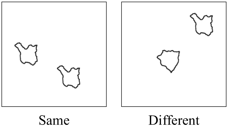
Figure 1: Same or different? For humans and a number of animal species, it is trivial to recognize that the image on the left contains two of the same objects, while the image on the right contains two different objects. Surprisingly, prior research has suggested that deep neural networks struggle to learn to discriminate between these images.

Humans and a wide variety of non-human animals can easily recognize whether two objects are the same as each other or whether they are different (see Figure 1; Martinho III & Kacelnik, 2016; Christie, 2021; Gentner et al., 2021; Hespos et al., 2021). The abstract concept of equality is simple—even 3-month-old infants (Anderson et al., 2018) and honeybees (Giurfa, 2021) can learn to distinguish between displays of two same or two different objects. Some researchers have even argued that it serves amongst a number of other basic logical operations as a foundation for higher-order cognition and reasoning (Gentner & Goldin-Meadow, 2003; Gentner & Hoyos, 2017). However, in contrast to humans and animals, recent work has argued that deep neural networks struggle to learn this simple relation (Ellis et al., 2015; Gülçehre & Bengio, 2016; Stabinger et al., 2016; Kim et al., 2018; Webb et al., 2020; Puebla & Bowers, 2022). This difficulty is surprising given that deep neural networks achieve human or superhuman performance on a wide range of seemingly more complex visual tasks, such as image classification (Krizhevsky et al., 2012; He et al., 2016), segmentation (Long et al., 2015), and generation (Ramesh et al., 2022).

Past attempts to evaluate same-different relations in neural networks have generally used the following methodology. Models are trained to classify images containing either two of the same or two different abstract objects, such as those in Figure 1. A model is considered successful if it is then able to generalize the same-different relation to unseen shapes after training. Convolutional neural networks (CNNs) trained from scratch fail to learn a generalizable relation, and tend to memorize training examples (Kim et al., 2018; Webb et al., 2020). However, deep neural networks have been shown to successfully generalize the same-different relation in certain contexts. This generalization is either limited to in-domain test stimuli (Funke et al., 2021; Puebla & Bowers, 2022) or requires architectural modifications that build in an inductive bias towards relational tasks at the expense of other visual tasks (Kim et al., 2018; Webb et al., 2020; 2023a; 2023b; Kerg et al., 2022; Geiger et al., 2023; Altabaa et al., 2023). Given these limited successes, an open question remains: without architectural modifications that restrict model expressivity in general, can standard neural networks learn an abstract same-different relation that generalizes to both in- and out-of-distribution stimuli?

Addressing this question requires going beyond past work in a number of ways. First, most previous studies test for in-distribution generalization—that is, they use test stimuli that are visually similar to the training stimuli. We believe that out-of-distribution generalization provides much stronger evidence that a model has learned a genuine abstract relation without relying on spurious features. Second, the existing literature uses training stimuli that demonstrate the same-different relation with either closed curves (as in Figure 1) or simple geometric shapes. It is unclear whether training on these types of objects is the most helpful for learning the relation versus more naturalistic objects that more closely resemble data seen during pretraining. Finally, most prior work focuses on convolutional architectures, but Vision Transformers (ViTs) (Dosovitskiy et al., 2020) adapted from the language domain (Vaswani et al., 2017) have recently emerged as a competitive alternative to CNNs on visual tasks. Self-attention, a key feature of ViTs, may provide an advantage when learning abstract visual relations—indeed, the ability to attend to and relate any part of a stimulus to any other part may be crucial for relational abstraction.

In this article, we address these limitations and comprehensively investigate how neural networks learn and generalize the same-different relation from image data. Our main findings are as follows:

• Fine-tuning pretrained ResNet and ViT models on the same-different relation enables both architectures to generalize the relation to unseen objects in the same distribution as the fine-tuning set. In particular, CLIP pretraining results in nearly $100\%$ in-distribution test accuracy for ViT models, and close to that for ResNet models. (Section 3.1)

• Under certain conditions, CLIP-pretrained ViTs can reliably generalize the same-different relation to out-of-distribution stimuli with nearly $100\%$ accuracy. This suggests that these models may acquire a genuinely abstract concept of equality. (Section 3.2)

• Different fine-tuning datasets lead to qualitatively different patterns of generalization—fine-tuning on more visually abstract objects (which do not contain color or texture) results in stronger out-of-distribution generalization, whereas fine-tuning on more naturalistic objects fails to generalize. (Section 3.2)

• ViTs generally prefer to determine equality between objects by comparing their color or texture, only learning to compare shape when the fine-tuning dataset lacks color and texture information. However, we find that CLIP pretraining helps to mitigate this preference for color and texture. (Section 4)

2 Methods

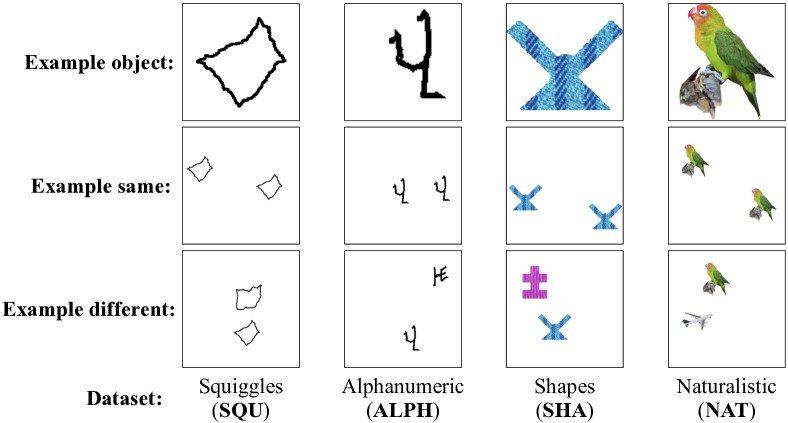
Figure 2: Example stimuli from all four datasets. Each column represents one of the four same-versus-different datasets as indicated by the label beneath the stimuli. The top row shows an example object that is used to form the stimuli that comprise each dataset, while the second and third rows show an example “same” vs. “different” stimulus, respectively.

We operationalize the same-different task consistently with prior work e.g. Fleuret et al. (2011). Models are asked to perform a binary classification task on images containing either two of the same objects or two different objects (see the second and third rows of Figure 2). Models are either trained from scratch or fine-tuned on a version of this task with a particular type of stimuli (see Section 2.1 below). After training or fine-tuning, model weights are frozen, and validation and test accuracy scores are computed on sets of same-versus-different stimuli containing unfamiliar objects. These can be either be the same type of objects that they were trained or fine-tuned on (in-distribution generalization) or different types of objects (out-of-distribution generalization). Thus, in order to attain high validation and test accuracy scores, the model must successfully generalize the learned same-different relation to novel objects. This type of generalization is more challenging than the standard image classification setting because of the abstract nature of what defines the classes—models must learn to attend to the relationship between two objects rather than learn to attend to any particular visual features of those objects in the training data.

2.1 Training and Evaluation Datasets

We construct four same-versus-different datasets using four different types of objects (see Figure 2) ranging from abstract shapes to naturalistic images that are more familiar to pretrained models. We use the following objects to create these four datasets:

1. Squiggles (SQU). Randomly generated closed shapes following Fleuret et al. (2011). Most studies in the machine learning literature on the same-different relation uses this dataset (Kim et al., 2018; Funke et al., 2021; Puebla & Bowers, 2022; Messina et al., 2022).

2. Alphanumeric (ALPH). Sampled handwritten characters from the Omniglot dataset (Lake et al., 2015).

3. Shapes (SHA). Textured and colored shapes from Tartaglini et al. (2022). Objects that match in shape, texture, and color are considered the same, whereas objects that differ along all three dimensions are considered different.

4. Naturalistic (NAT). Photographs of real objects on white backgrounds from Brady et al. (2008). These stimuli are the most similar to the data that the pretrained models see before fine-tuning on the same-different task.

Each stimulus is an image that contains two objects that are either the same or different. We select a total of 1,600 unique objects for each dataset. These objects are split into disjoint sets of 1,200, 300, and 100 to form the training, validation, and test sets respectively. Unless otherwise specified, the training, validation, and test sets each contain 6,400 stimuli: 3,200 same and 3,200 different. To construct a given dataset, we first generate all possible pairs of same or different objects—we consider two objects to be the same if they are the same on a pixel level. Next, we randomly select a subset of the possible object pairs to create the stimuli such that each unique object is in at least one pair. Each object is resized to 64x64 pixels, and then a pair of these objects is placed over a 224x224 pixel white background in randomly selected, non-overlapping positions. We consider two objects in a specific placement as one unique stimulus—in other words, a given pair of objects may appear in multiple images but in different positions (but with all placements of the same two objects being confined to either the training, validation, or test set). All object pairs appear the same number of times to ensure that each unique object is equally represented.

2.2 Models and Training Details

We evaluate one convolutional architecture, ResNet-50 (He et al., 2016), and one Transformer architecture, ViT-B/16 (Dosovitskiy et al., 2020). We also evaluate three pretraining procedures: (1) randomly initialized, in which all model parameters are randomly initialized (Kaiming normal for ResNet-50 and truncated normal for ViT-B/16) and models are trained from scratch, (2) ImageNet, in which models are pretrained in a supervised fashion on a large corpus of images (ImageNet-1k for ResNet-50 and ImageNet-21k for ViT-B/16; Deng et al., 2009) with category labels such as “barn owl” or “airplane,” and (3) CLIP (Radford et al., 2021), in which models learn an image-text contrastive objective where the cosine similarity between an image embedding and its matching natural language caption embedding is maximized. Unlike ImageNet labels, CLIP captions contain additional linguistic information beyond category information (e.g. “a photo of a barn owl in flight”). To adapt these models for the same-different task, we add a randomly initialized linear classifier on top of the visual backbone of the original architecture.

Each model is trained from scratch or fine-tuned for 70 epochs with a batch size of 128, updating all parameters. We use a binary cross-entropy loss. For each architecture and pretraining combination, we perform hyperparameter tuning via grid search over the initial learning rate (1e-4, 1e-5, 1e-6, 1e-7, 1e-8), learning rate scheduler (exponential, ReduceLROnPlateau), and optimizer (SGD, Adam, AdamW). We select the best performing training configuration from the grid search according to in-distribution validation accuracy, and then train a model with those hyperparameters five times with different random seeds. We report the median test results across those five seeds.

3 Generalization to Unseen Objects

3.1 In-Distribution Generalization

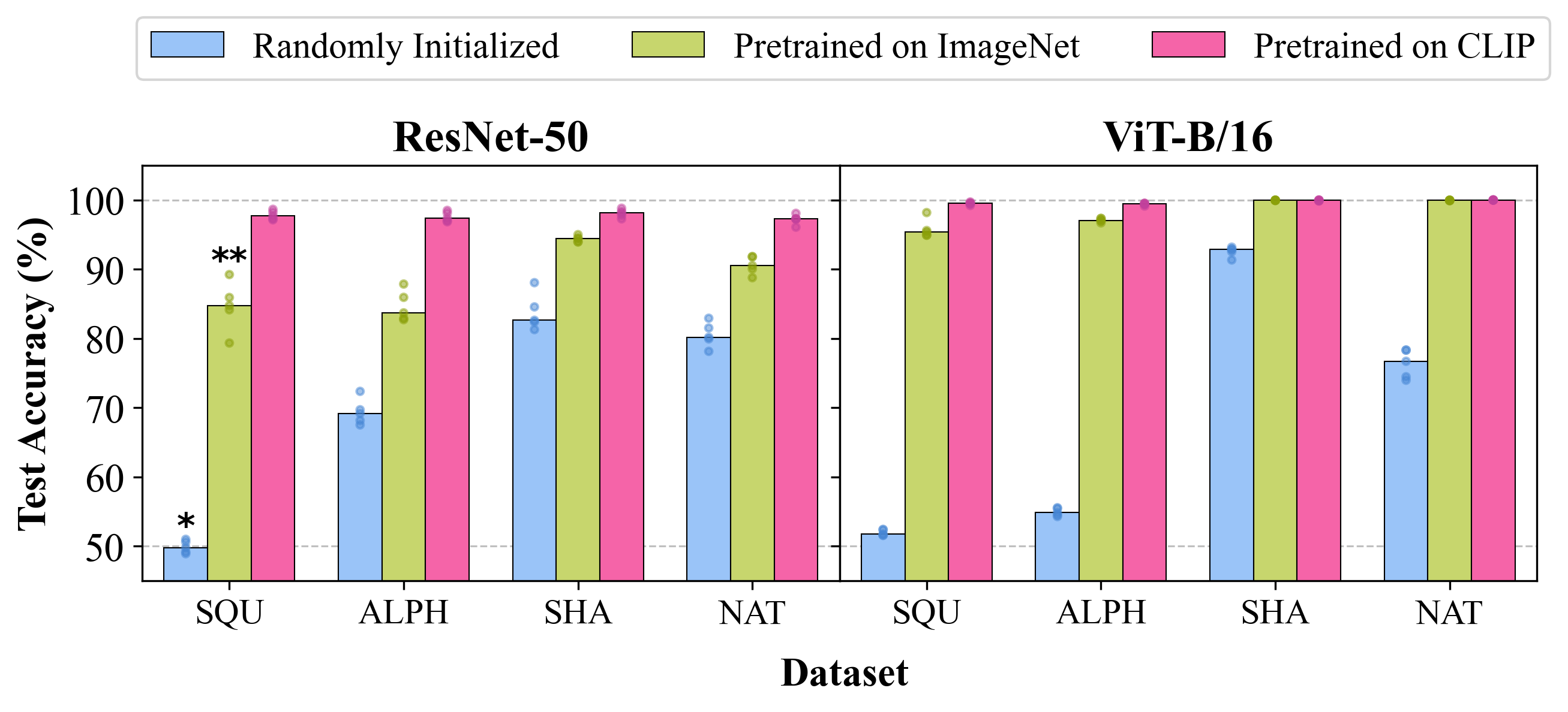
Figure 3: In-distribution test accuracy by architecture and pretraining method. Bars show median accuracy over 5 runs (individual points also shown), with the bar color denoting pretraining type and the x-axis denoting the dataset used for fine-tuning. See Section 2.1 for dataset descriptions, Section 2.2 for model details, and Figure 2 for visual examples. The starred ($*$) result is a replication of findings from prior work showing that CNNs trained from scratch on stimuli like the images in Figure 1 attain chance-level test accuracy. The double-starred ($**$) result mirrors Funke et al. (2021) and Puebla & Bowers (2022), who show that ImageNet-pretrained CNNs attain substantially higher in-distribution test accuracy relative to the same architectures trained from scratch.

We first measure the performance of each model on test data containing the same types of objects used to train or fine-tune the model; e.g. models fine-tuned on pairs of handwritten characters are then tested on handwritten characters that were not seen during training. We refer to this as the in-distribution performance of the model. The starred ($*$) result in Figure 3 shows the in-distribution median test accuracy of randomly-initialized ResNet-50 models trained on the Squiggles dataset, which contains the same type of closed contours used by much of the prior work on the same-different relation (Fleuret et al., 2011; Kim et al., 2018; Funke et al., 2021; Puebla & Bowers, 2022; Messina et al., 2022). Confirming the primary findings from prior work, these models do not attain above chance level test accuracy. The same pattern holds for randomly initialized ViT-B/16 models.

However, as the rest of Figure 3 shows, pretrained models exhibit substantially improved in-distribution accuracy compared to randomly initialized models across all four datasets. In particular, models pretrained with CLIP demonstrate the largest improvements, attaining nearly $100\%$ test accuracy irrespective of fine-tuning dataset. Even without any fine-tuning, CLIP features appear to be highly useful for the same-different task—linear probes trained to do the same-different task using CLIP ViT-B/16 embeddings of stimuli without any fine-tuning achieve between $80\%$ and $100\%$ median in-distribution test accuracy depending on the dataset (Table 10, Appendix A.5). Differences in performance can also be observed between architectures, with ViT-B/16 models consistently outperforming ResNet-50 after pretraining.

Another main finding is that the two visually abstract, shape-based datasets (Squiggles and Alphanumeric) appear to pose more of a challenge to models than the Shapes and Naturalistic datasets—models attain noticeably higher in-distribution accuracy on the latter two across architectures and pretraining methods (although the effect is small for CLIP-pretrained models). This difference may be due to the color and texture information that is available in these datasets, which provides additional dimensions over which objects can be compared. We explore the possibility that some models find it easier to evaluate equality using color and texture information in addition to or instead of shape information in Section 4.

3.2 Out-of-Distribution Generalization

The previous section showed that pretrained models can generalize to unseen, in-distribution objects. However, if a model learns a truly abstract notion of same-different, it should generalize the same-different relation to any two objects regardless of their particular visual features. Thus, model performance on stimuli that are substantially different from training stimuli is a stronger measure of abstraction. We therefore measure test accuracy for each model across all four datasets, yielding one in-distribution score and three out-of-distribution (OOD) scores per model. Table 1 shows median test accuracy over five seeds for CLIP-pretrained models; full generalization tables for all pretraining styles and architectures can be found in Appendix A.2.

Overall, CLIP ViT-B/16 models fine-tuned on the Squiggles task exhibit the strongest OOD generalization, achieving $>$95% median test accuracy on the three out-of-distribution datasets. It is worth noting that both this model and CLIP ResNet-50 fine-tuned on the Alphanumeric task (the model with the second best OOD generalization performance) exhibit some degree of sensitivity to the random seed used during fine-tuning: most random seeds result in nearly $100\%$ OOD generalization for ViT or $>$80% for ResNet across all datasets, while some seeds result in substantially lower performance (1/5 seeds for ViT and 2/5 for ResNet). No other model configurations exhibit this bimodal behavior. See Appendix A.8 for details.

As in the previous section, models fine-tuned on objects with visually abstract shape features only (Squiggles and Alphanumeric) behave differently than those fine-tuned on datasets containing objects with shape, color, and texture features (Shapes and Naturalistic). The Squiggles and Alphanumeric models generally attain high OOD test accuracy. On the other hand, models fine-tuned on the Shapes or Naturalistic datasets generalize well to each other but struggle to generalize to the Squiggles and Alphanumeric tasks. Note that some of this effect can be attributed to miscalibrated bias, but not the entire effect—see Appendix A.3 for details.

CLIP ResNet-50
	$\leftarrow$ Test $\rightarrow$
Train $\downarrow$	SQU	ALPH	SHA	NAT	Avg.
SQU	97.7	82.9	86.9	82.0	83.9
ALPH	82.1	97.4	92.8	91.8	88.9
SHA	56.0	78.1	98.1	96.1	76.7
NAT	50.1	59.3	93.4	97.3	67.6
Avg.	62.7	73.4	91.1	90.0

CLIP ViT-B/16
	$\leftarrow$ Test $\rightarrow$
Train $\downarrow$	SQU	ALPH	SHA	NAT	Avg.
SQU	99.6	97.7	99.1	96.7	97.8
ALPH	55.3	99.4	99.6	91.2	82.0
SHA	50.0	55.4	100	100	68.5
NAT	50.0	68.0	99.8	100	72.6
Avg.	51.8	73.7	99.5	95.9

Table 1: Out-of-distribution (OOD) test accuracy for CLIP models fine-tuned on each dataset. Rows indicate the dataset that models are fine-tuned on, while columns indicate the test dataset. Each cell is the median performance over five random seeds. The rightmost column labeled “Avg.” is the row-wise average of accuracy scores across OOD test sets (i.e. off-diagonal values), which indicates how well a model fine-tuned on a given dataset is able to generalize to other datasets. The bottom row labeled “Avg.” is the column-wise average across off-diagonal values, indicating how difficult it is for models fine-tuned on other datasets to generalize to the given dataset. Note that the bolded diagonals are the red bars in Figure 3. OOD generalization results for all model architectures and pretraining styles can be found in Appendix A.2; Appendix A.3 shows median AUC-ROC scores.

Another way to understand the generalization pattern in Table 1 is that the more “challenging” a dataset is to generalize the same-different relation to, the more effective it is as a fine-tuning dataset for inducing out-of-distribution generalization. For example, CLIP ViT-B/16 models fine-tuned on datasets other than Squiggles attain a median test accuracy of only $51.8\%$ on the Squiggles task on average, whereas CLIP ViT-B/16 fine-tuned on Squiggles attains an average OOD test accuracy of $97.8\%$. On the other hand, the Shapes dataset is easy for models fine-tuned on other datasets to generalize to ($99.5\%$ accuracy on average), but CLIP ViT fine-tuned on that “easier” dataset attains an average OOD test accuracy of only $68.5\%$. This pattern of Squiggles being more “difficult” to generalize to persists across architectures and pretraining methods (Appendix A.2).

Dataset $\downarrow$	ResNet-50	ViT-B/16
noise	0.992	0.993
SQU	0.929	0.940
ALPH	0.881	0.889
SHA	0.855	0.861
NAT	0.788	0.805

Table 2: Average pairwise cosine similarity between CLIP embeddings of training stimuli within each dataset. Because $n=6,400$ for each dataset, averages are computed over approximately 20M pairs. We extract CLIP embeddings before fine-tuning on the same-different task. For similarities afterwards, see Appendix A.6.

We further study why fine-tuning on different datasets results in different generalization behaviors by computing the average cosine similarity between objects in a given dataset using pretrained CLIP embeddings (Table 2) . This value provides information about the visual variation in each dataset through the lens of a specific model: a higher number means that stimuli in that dataset are generally embedded more closely together by that model. Before fine-tuning, pretrained CLIP models embed Squiggles stimuli more closely together than stimuli from other datasets, potentially explaining the difficulty of that dataset as a test of OOD generalization. We also note what seems to be a correlation between “closeness” of stimuli in a model’s embedding space and ability of models fine-tuned on that dataset to generalize OOD. Given that random noise is embedded even more closely together than Squiggles stimuli, we fine-tune models on the same-different task comparing patches of random noise and measure their OOD generalization in Appendix A.7. We find that models fine-tuned on noise exhibit weaker OOD generalization than models fine-tuned on Squiggles, indicating that “closeness” of stimuli is not a perfect correlate of OOD generalization and is only part of the story.

4 Examination of Inductive Biases

4.1 Grayscale and Graymasked Objects

What features are most important for learning a genuinely abstract same-different relation, and do vision models have inductive biases towards these useful features? Previous work has claimed that CNN models trained on ImageNet are often biased towards texture over shape (Geirhos et al., 2019; Hermann et al., 2020), which seems consistent with results from Kim et al. (2018) showing low performance for CNNs trained from scratch on abstract shapes. Based on the results in the previous section, shape information appears to be the most important for effective OOD generalization, which motivates us to investigate whether models have an inductive bias towards it for the visual same-different task. One way of examining this is by training models on one of three variants of the Shapes dataset: objects are either kept the same (Figure 4a, “Colored”), grayscaled to preserve texture but remove color (Figure 4a, “Grayscale”), or completely masked over in gray to remove both texture and color (Figure 4a, “Masked”). If a model is biased towards color, we would expect performance to drop on the Grayscale and Masked datasets, and if it is biased towards texture, we would expect performance to suffer on the Masked dataset. Only a model biased towards shape would generalize effectively to all three settings.

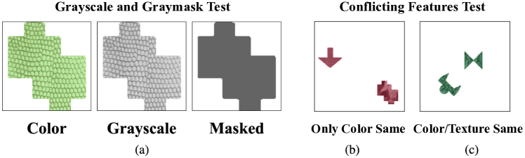
Figure 4: Examples of stimuli used to test inductive biases. Figure (a) shows examples of objects from the three versions of the Shapes dataset used to produce results in Figure 5. Figures (b) and (c) are examples of stimuli with conflicting signals used in Section 4.2, where either color is the same while texture and shape are different, or color and texture are the same while shape is different.

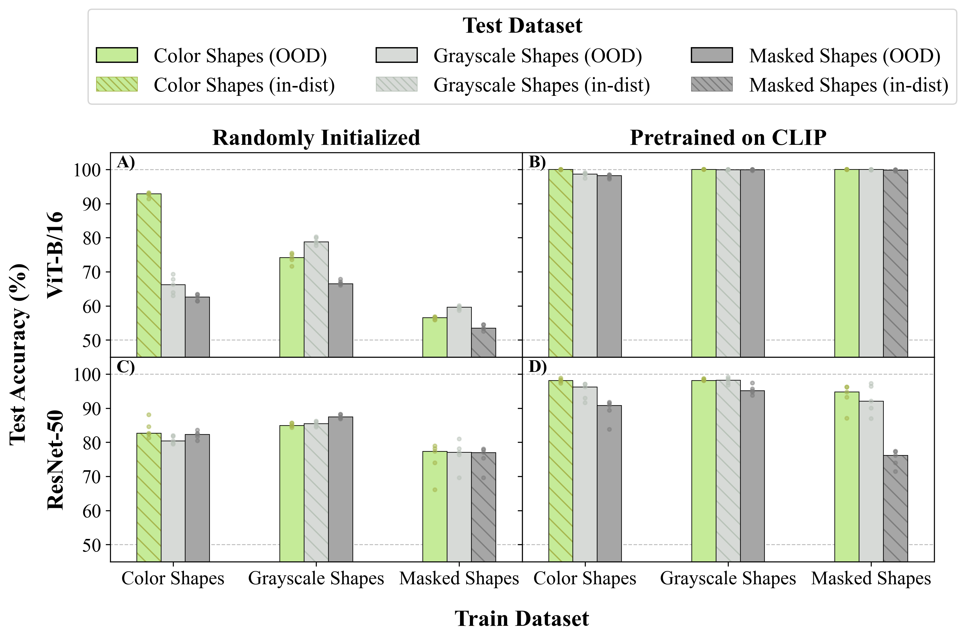
Figure 5: Test accuracy for ViT-B/16 fine-tuned on one version of the Shapes dataset – Color, Grayscale, or Masked – and tested on all three datasets. See Figure 4a for example objects from each of the three datasets. Bars are grouped by fine-tuning dataset as indicated along the x-axis. Hatched bars indicate in-distribution accuracy. Median accuracy over five seeds is reported with individual runs plotted as points over each bar. See Appendix B.1 for ImageNet and ResNet results.

Figure 5 shows the results of this experiment for randomly initialized and CLIP-pretrained models (ImageNet results in Appendix B.1). Figure 5A shows the test performance of three versions of randomly initialized ViT-B/16, trained on either Color, Grayscale, or Masked versions of the Shapes dataset (Figure 4a) and then tested on novel objects from each of those distributions. From this subplot, we can see that ViT-B/16 trained from scratch can only achieve high in-distribution accuracy (shown as hatched bars) for Color Shapes ($92.9\%$); the hatched gray and dark gray bars representing in-distribution accuracy for Grayscale and Masked Shapes are much lower ($78.8\%$ and $53.5\%$ respectively). Although ViTs trained from scratch on the Color Shapes dataset attain high in-distribution accuracy, performance drops to $66.2\%$ and $62.6\%$ when generalizing out-of-distribution to Grayscale and Masked Shapes, indicated by the two lower gray bars beside the hatched green bar. This gap suggests that ViT-B/16 may only learn to compare object color when it is trained from scratch on the Color Shapes dataset, leading to greater errors when tested on datasets that do not contain color. Figure 5B shows that CLIP pretraining weakens this inductive bias towards color, allowing for high in-distribution accuracy and near-perfect out-of-distribution generalization when trained on any of the three modified Shapes datasets.

When ResNet-50 is trained from scratch, we do not see evidence of an inductive bias towards color or texture, since bars of all colors in Figure 5C are at roughly equal heights. However, this bias reappears after pretraining (albeit to a lesser extent than for randomly-initialized ViT), with a $7.3\%$ gap between in-distribution and Masked OOD accuracy for CLIP ResNet-50 fine-tuned on Color Shapes (Figure 5D).

4.2 Dissociating Color, Texture, and Shape

Results from Figure 5 suggest that some models learn to rely on certain features more than others to differentiate between objects in an image. We run an additional experiment to verify these claims by creating new stimuli for which color, texture, and shape send conflicting signals: for example, two objects in an image might be the same color but have different textures and shapes (Figure 4b). We then evaluate each model from Figure 5 on every possible combination of conflicting signals according to experiment details in Appendix B.2 to identify which features each model might be more biased towards. Median results are reported across five random seeds for the same set of hyperparameters. First, our results confirm that randomly-initialized ViT-B/16 is heavily biased towards color when trained on the Color Shapes dataset. When trained completely from scratch on Color Shapes, ViT-B/16 will predict “same” for any stimuli in which the colors of the two objects are the same, even if color is the only similarity between the two objects (classifying $85.6\%$ of stimuli like Figure 4b as “same”). In contrast, CLIP ViT-B/16 fine-tuned on the same Color Shapes data classifies only $12.3\%$ of stimuli like Figure 4b as “same.” However, our results also show that even CLIP ViT-B/16, which appears to be unbiased, exhibits different patterns of behavior depending on the dataset it is fine-tuned on. When tested on stimuli where color and texture are the same and shape is different (Figure 4c), CLIP ViT-B/16 fine-tuned on Color Shapes classifies $88.8\%$ of these stimuli as “same.” The same model fine-tuned on Masked Shapes classifies $98.2\%$ of these images as “different.” All results can be found in Appendix B.2.

A similar phenomenon can be observed in pretrained ResNet-50 models. For example, CLIP ResNet-50 fine-tuned on Masked Shapes exhibits a strong bias towards shape, classifying $\geq 89.8\%$ of objects with matching shapes as “same” while classifying $\geq 93.3\%$ of objects with mismatching shapes as “different.” Thus, even though pretraining can mitigate the strength of ViT inductive biases, all pretrained architectures still exhibit specific, understandable biases that are determined by the features available in their training data. Moreover, these distinct patterns of generalization provide a glimpse into how these networks are computing same-versus-different judgments.

5 Related Work

Prior work on the same-different relation. Learning the same-different relation when the two objects being compared occupy the same image appears to be the most challenging setting for deep neural networks. Most closely related to our work is Puebla & Bowers (2022). Their setup is very similar to ours in a few respects: they define the same-different task identically to us, fine-tuning ImageNet pretrained ResNet-50 models on the task using stimuli from Fleuret et al. (2011) (which are nearly identical to our Squiggles stimuli), and testing OOD generalization on nine evaluation sets. They find that their models fail to generalize out-of-distribution and draw the conclusion that current CNNs are unable to learn the relation. Replicating their setup, we find that the difference in our results is due to the differing architectures and pretraining methods we investigated. Our ImageNet ResNet-50 model fine-tuned on Squiggles also struggles to generalize to the evaluation sets used in Puebla & Bowers (2022), but our CLIP ViT-B/16 model fine-tuned on Squiggles generalizes perfectly or nearly perfectly to seven out of nine of these sets. See Appendix A.4 for details. Additionally, Funke et al. (2021) report that ImageNet pretrained ResNet-50 models fine-tuned on stimuli from Fleuret et al. (2011) can generalize the relation to in-distribution test stimuli in this setting, but OOD generalization is not tested. The double-starred ($**$) bar in Figure 3 replicates their results. Messina et al. (2022) show that a recurrent, hybrid CNN+ViT can attain high in-distribution test accuracy when objects occupy the same image, while (Webb et al., 2023b) demonstrate success using slot attention to segment the objects. Otherwise, successful generalization of the same-different relation with deep neural networks has been limited to a setting where objects are segmented into two separate inputs by humans and separately passed into a neural network (Kim et al., 2018; Webb et al., 2020; Kerg et al., 2022; Altabaa et al., 2023; Geiger et al., 2023).

Abstract relation learning. More generally, our work relates to a larger body of work concerned with the abilities of deep neural networks to learn abstract relations. The ability to abstract from sparse sensory data is theorized to be fundamental to human intelligence (Tenenbaum et al., 2011; Ho, 2019) and is strengthened by the acquisition of language (Gentner & Hoyos, 2017). In contrast, standard deep neural networks often struggle to learn relational reasoning from sensory data alone, even when the training corpus is very large (Mitchell, 2021; Davidson et al., 2023). This is often pointed to as a key discrepancy between human and machine visual systems.

6 Discussion and Conclusion

Previous work has argued that deep neural networks struggle to learn the same-different relation between two objects in the same image (Kim et al., 2018; Puebla & Bowers, 2022), but the scope and nature of these difficulties are not fully understood. In this article, we explored a range of architectures, pretraining styles, and fine-tuning datasets in order to thoroughly investigate the ability of neural networks to learn and generalize the same-different relation. Some of our model configurations are able to generalize the relation across all of our out-of-distribution evaluation datasets; the best model is CLIP-pretrained ViT fine-tuned on the Squiggles same-different task. Across five random seeds, this model yields a median test accuracy of nearly $100\%$ on every evaluation dataset we use. The existence of such a model suggests that deep neural networks can learn generalizable representations of the same-different relation, at least for the tests we examined.

There are a number of possible reasons why CLIP-pretrained Vision Transformers exhibit the strongest out-of-distribution generalization. CLIP pretraining may be helpful because of the diversity of the dataset, which Fang et al. (2022) argue is key in the robust generalization of CLIP models in other settings. Another hypothesis is that linguistic supervision from captions containing phrases like “same,” “different,” or “two of” (which ImageNet models would have no exposure to) helps models to separate same and different objects in their visual embedding spaces, an idea supported by the results of our linear probe experiments (Appendix A.5). ViTs may perform the best on the same-different task because of their larger receptive field size; CNNs can only compare distant image patches in deeper layers, whereas ViTs can compare any image patch to any other as early as the first self-attention layer. Thus, ViTs may be able to integrate complex shape information and compare individual objects to each other more efficiently than CNNs.

What mechanisms enable certain models to generalize the same-different relation? It is possible that models learn an internal circuit (e.g. Nanda et al. (2023)) in which they segment two objects and compute their equality in embedding space, implicitly implementing the components of relational architectures from earlier works that explicitly separate objects. This would amount to true abstraction and would theoretically enable models to generalize to any distribution of same-different stimuli. Indeed, CLIP ViT-B/16 also generalizes with near perfect accuracy to multiple evaluation sets used in other work (see Appendix A.4). Since our results strongly suggest that neural networks can learn generalizable same-different relations, the next step for future work is to investigate the internal workings of successful models. We believe that further progress in understanding abstraction ought to come from circuit-level investigations into the same-different relation, as well as other abstract visual relations. Such investigations may reveal additional relational reasoning capabilities that have long been considered out of reach for standard deep neural networks.

Appendix A Additional Generalization Results

A.1 In-Distribution Learning Curves

For each architecture and pretraining method, we plot loss and in-distribution validation accuracy per epoch of fine-tuning or training on each dataset. Lines show averages for the same set of hyperparameters (for that model+dataset) across five seeds.

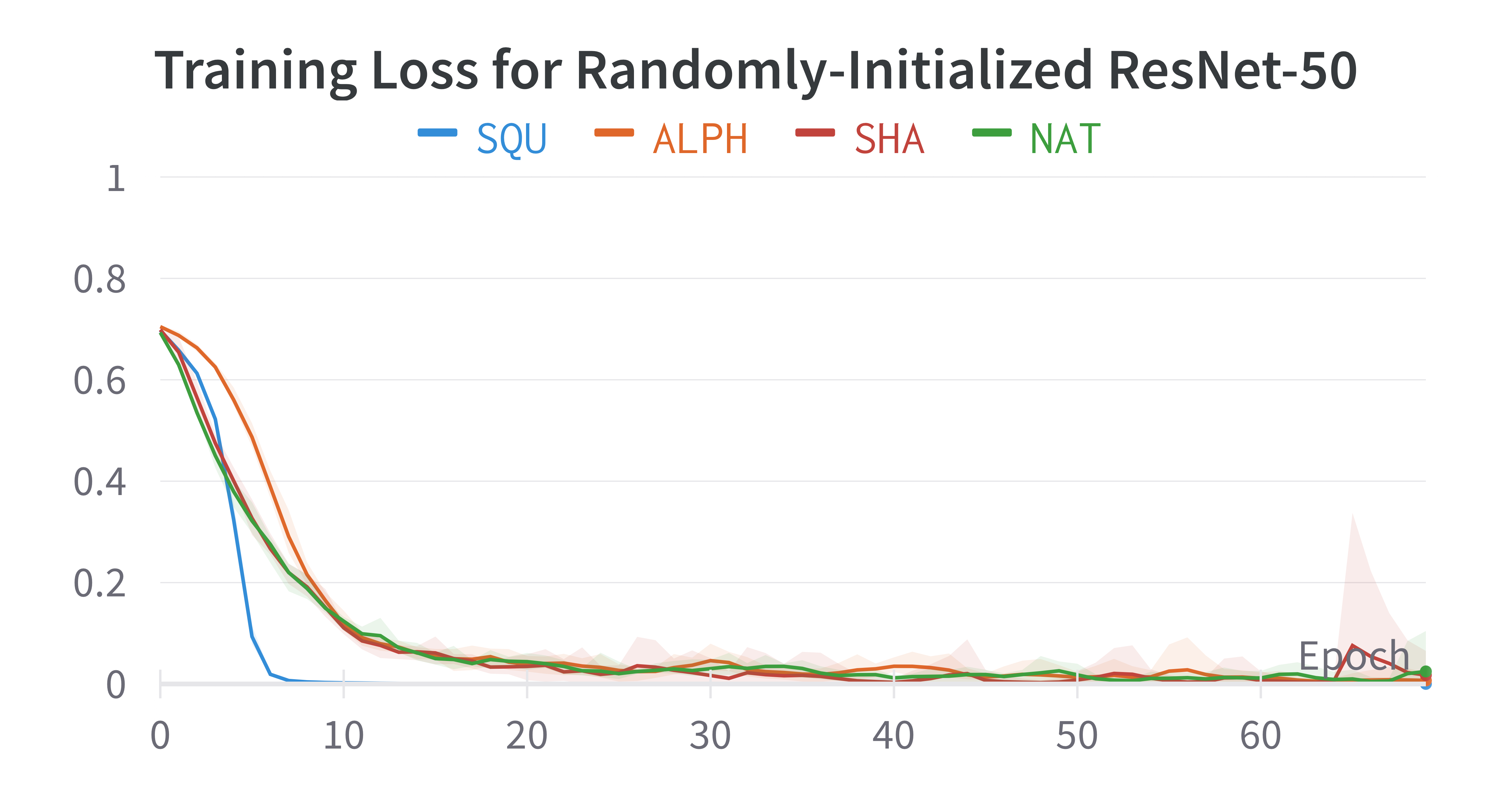
(a)

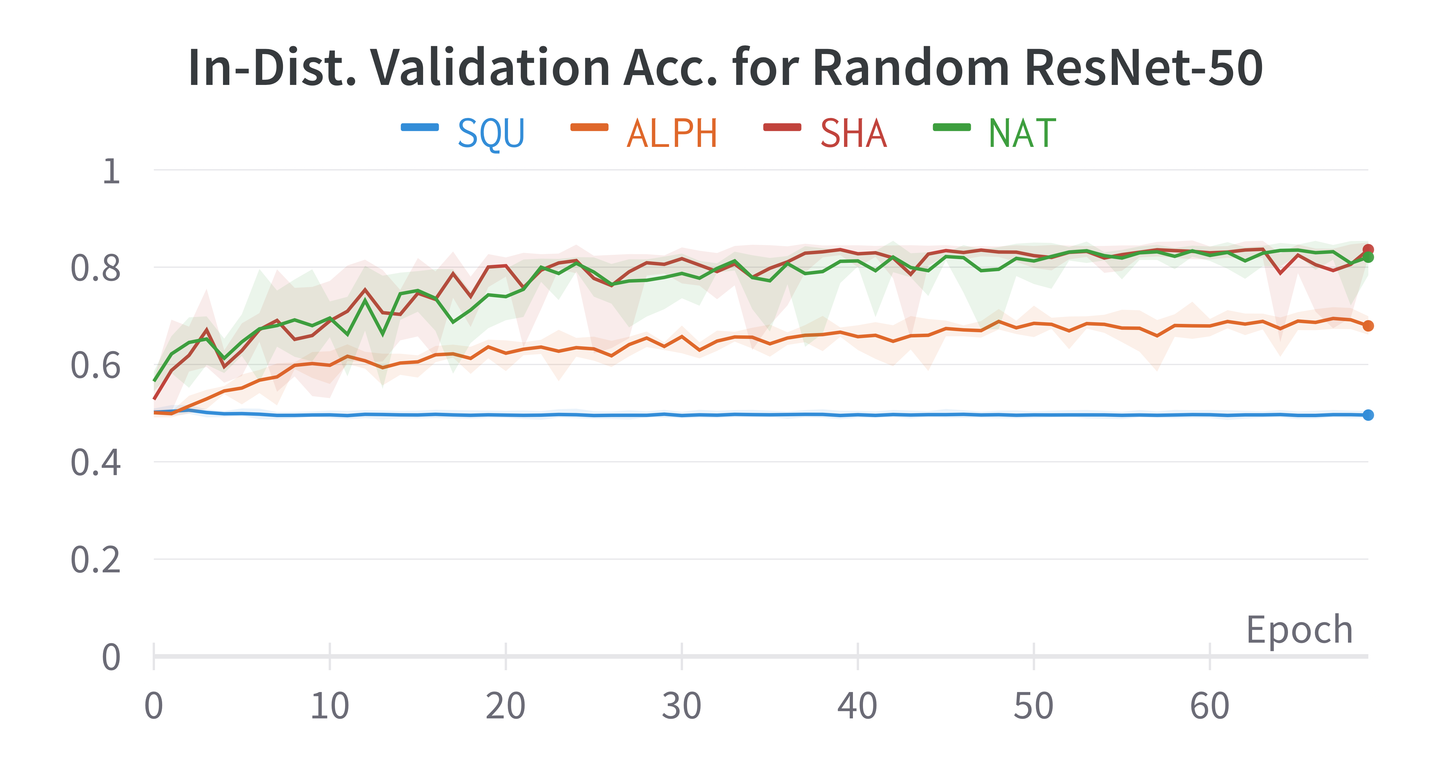
(b)

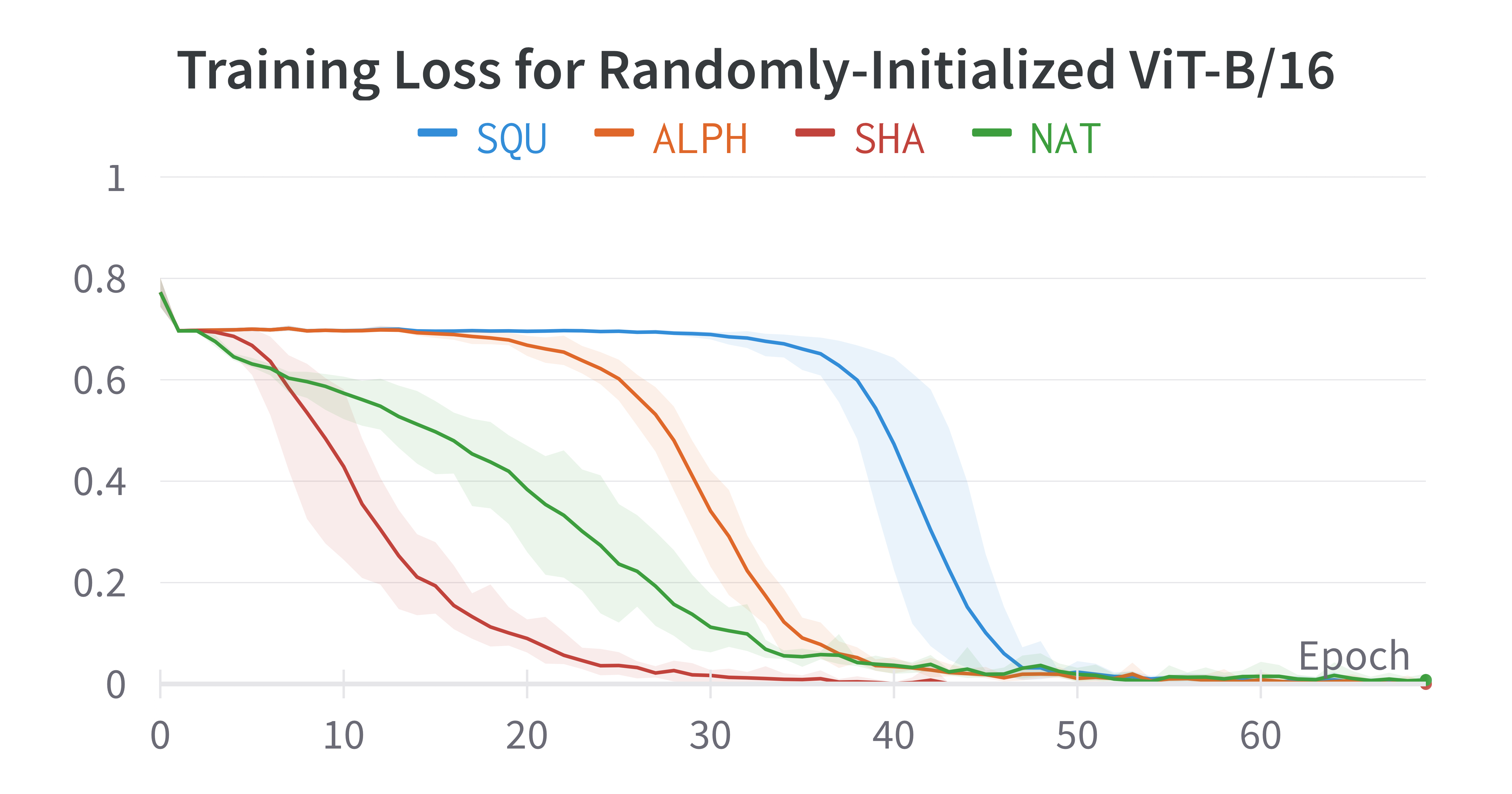
(c)

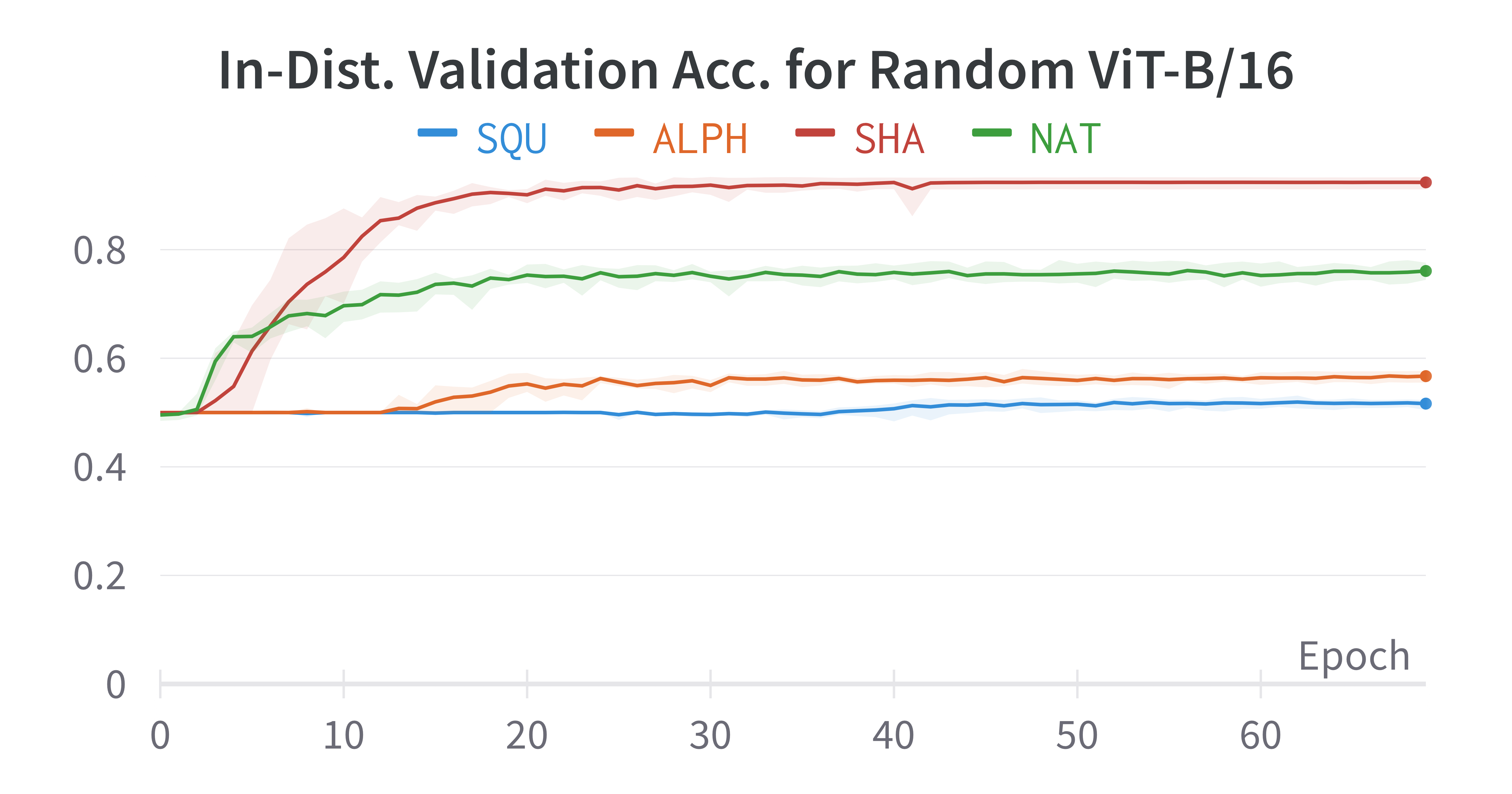
(d)

Figure 6: Average loss curves for randomly-initialized ResNet-50 and ViT-B/16 trained on each dataset. Even though loss curves for models trained on SQU go to zero, validation accuracy remains flat, indicating that models memorize training data. Furthermore, the loss curves for randomly-initialized ViT-B/16 distinctly mirror the hierarchy of dataset difficulty discussed in Section 3.2.

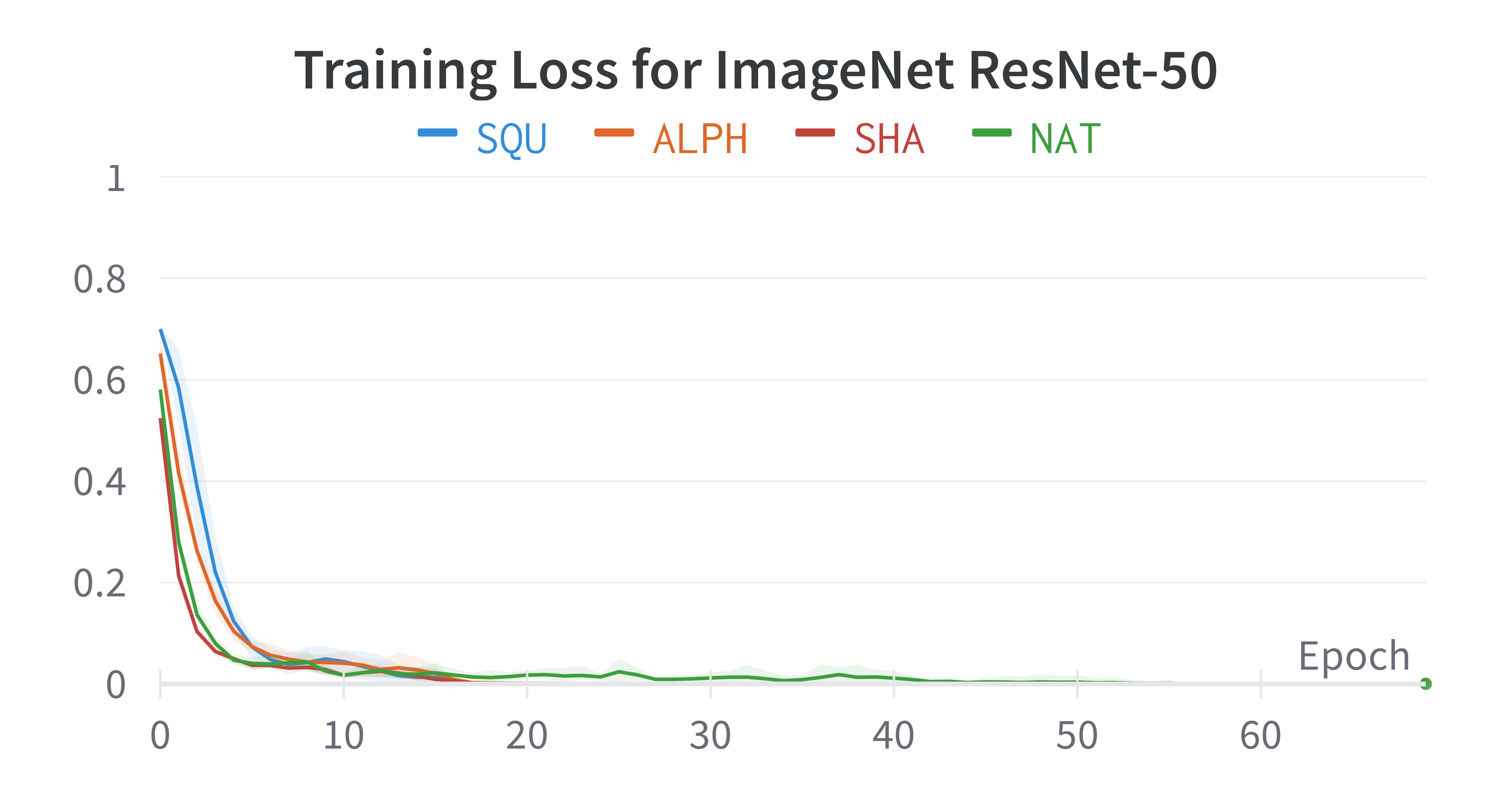
(a)

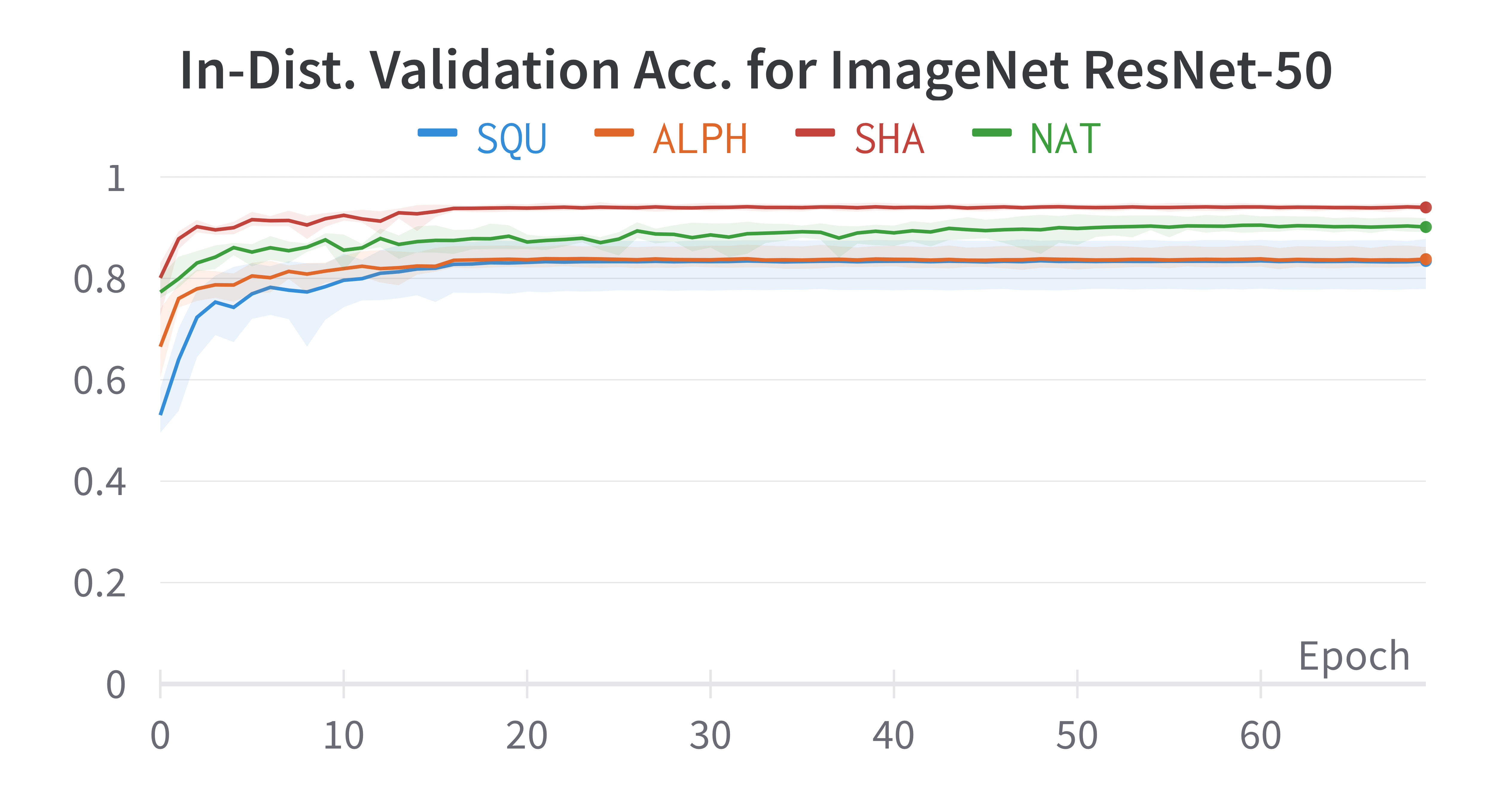
(b)

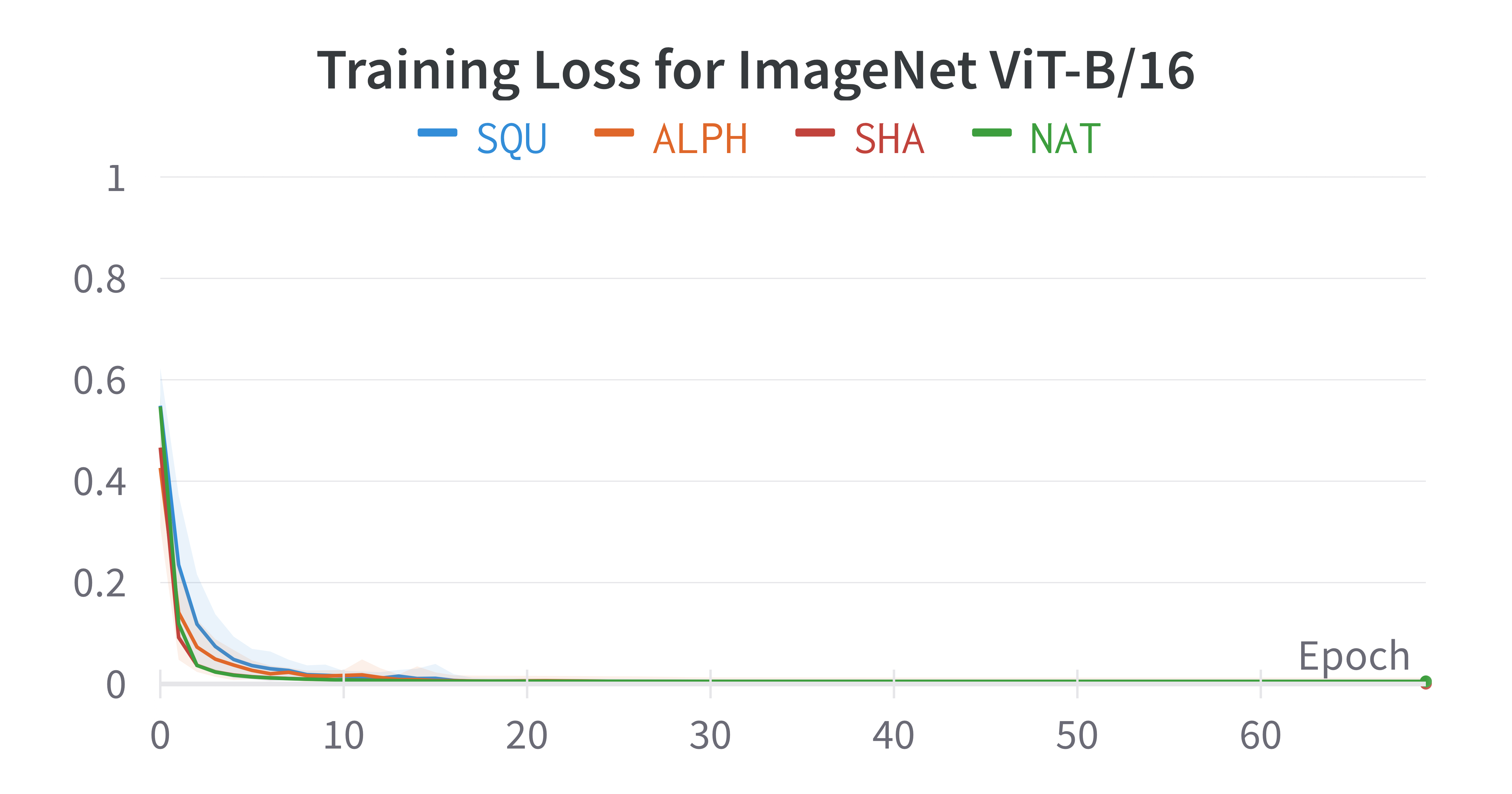
(c)

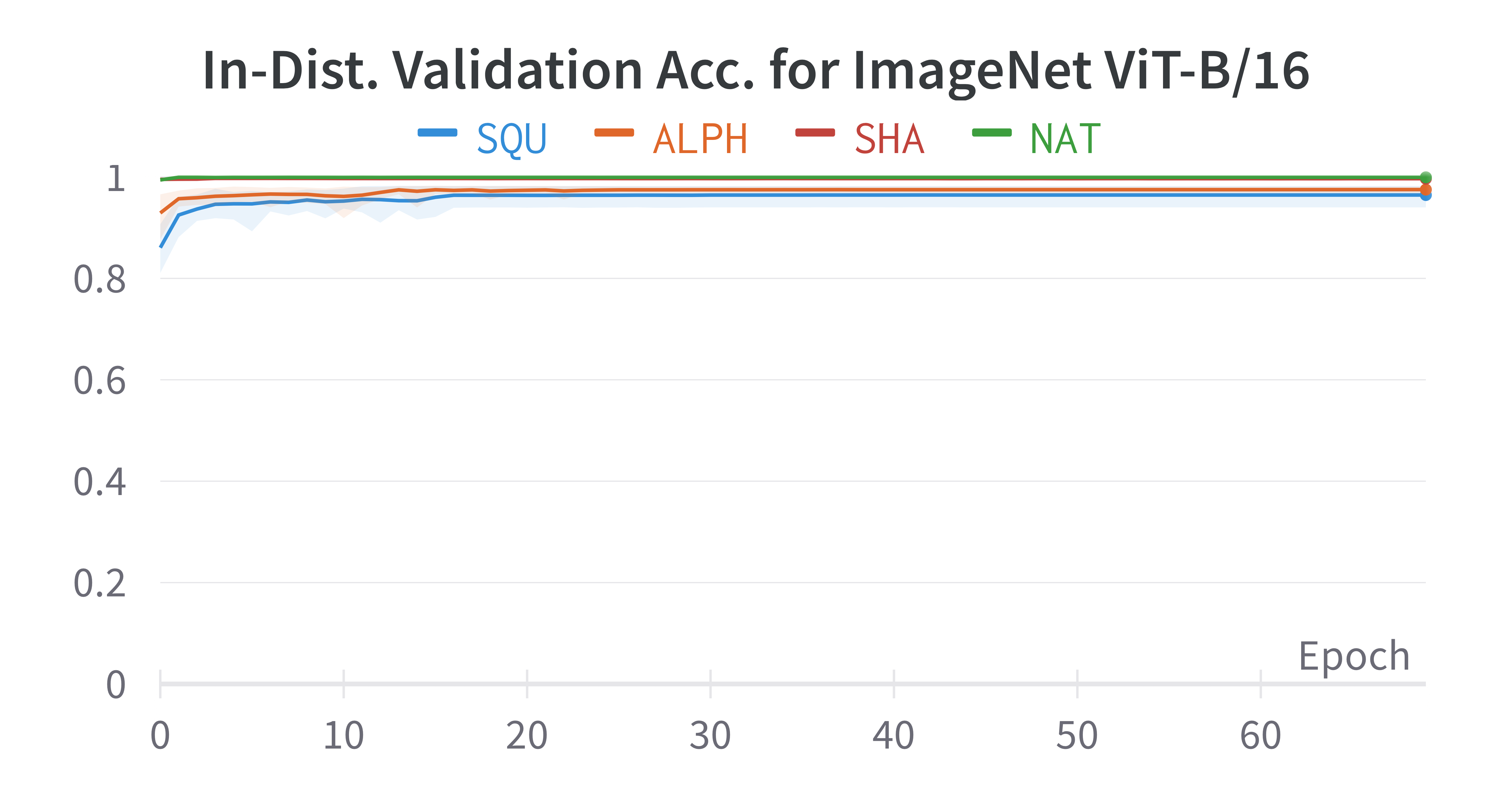
(d)

Figure 7: Average loss curves for ImageNet-pretrained ResNet-50 and ViT-B/16 fine-tuned on each dataset. Models converge substantially faster than in Figure 6. ImageNet ViT-B/16 models fine-tuned on SHA and NAT already attain nearly 100% validation accuracy after only one epoch.

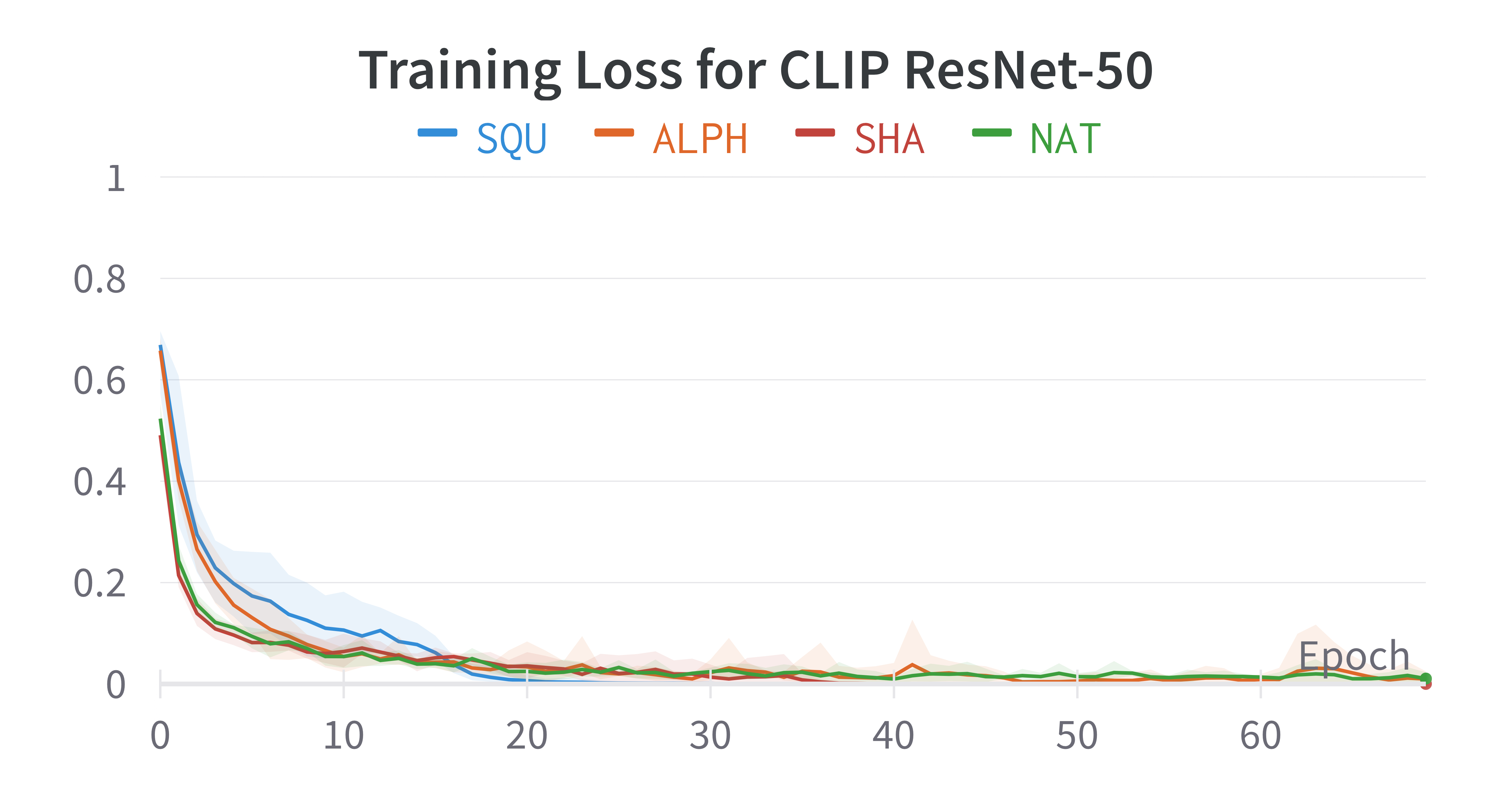
(a)

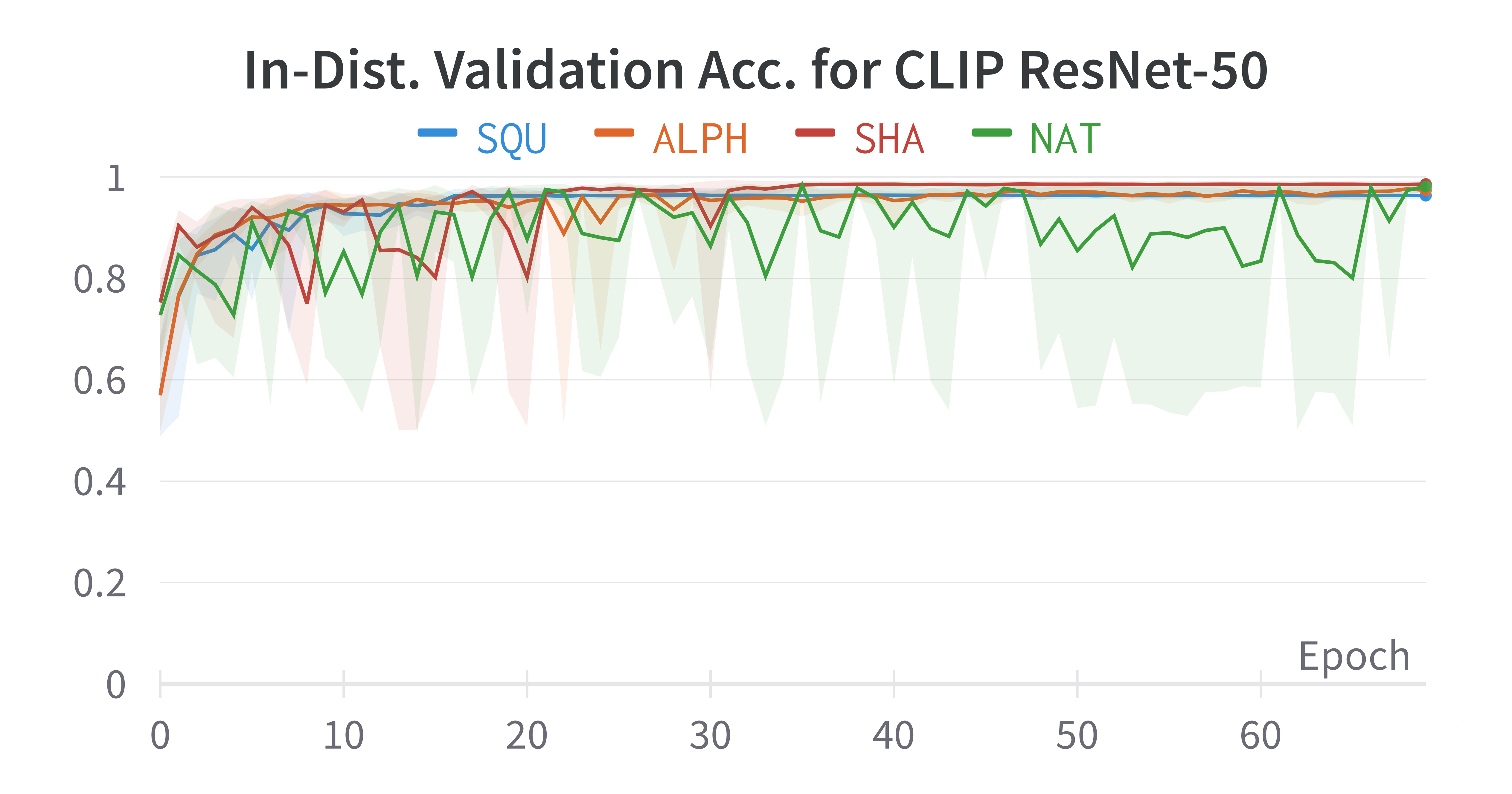
(b)

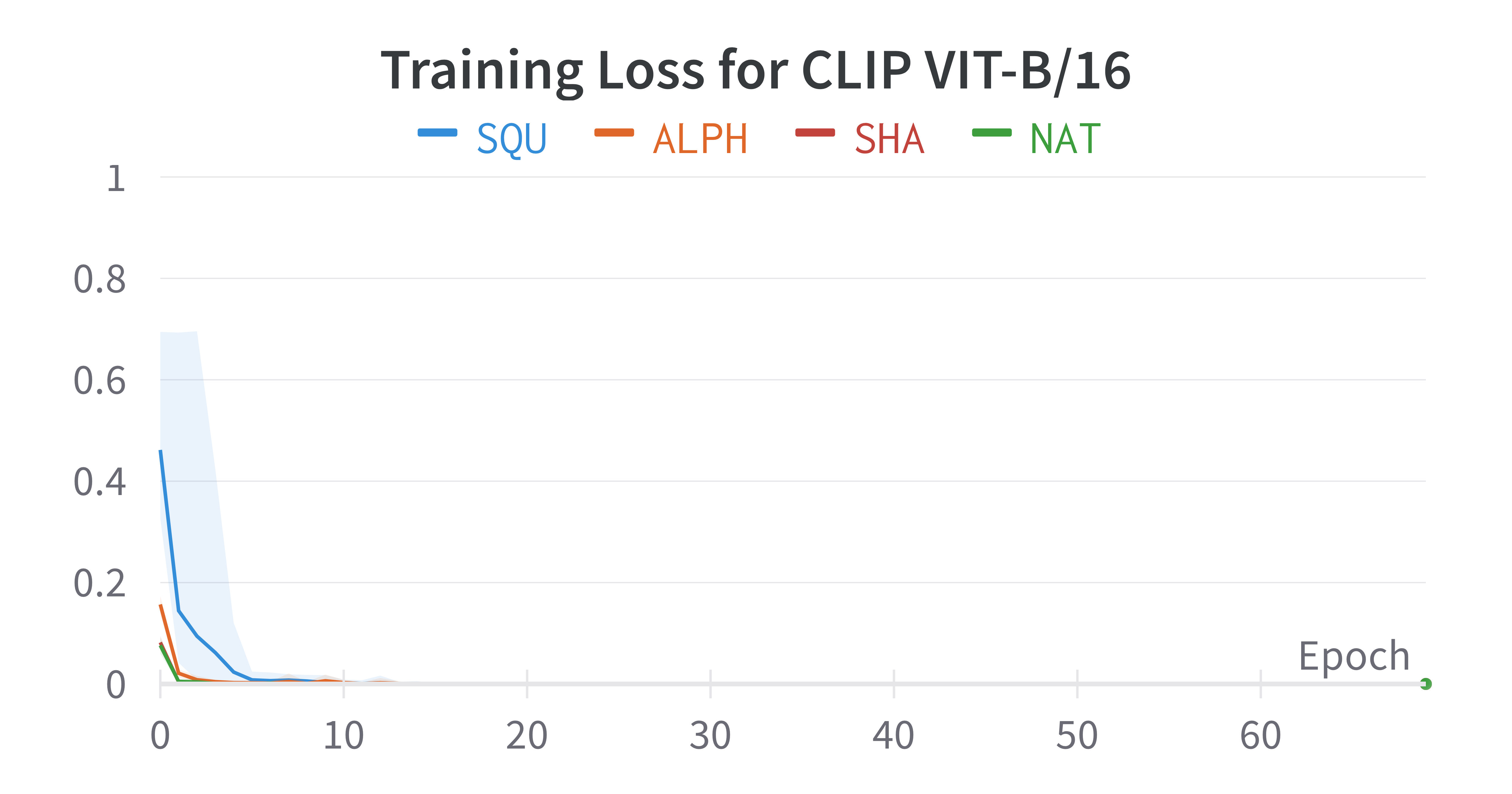
(c)

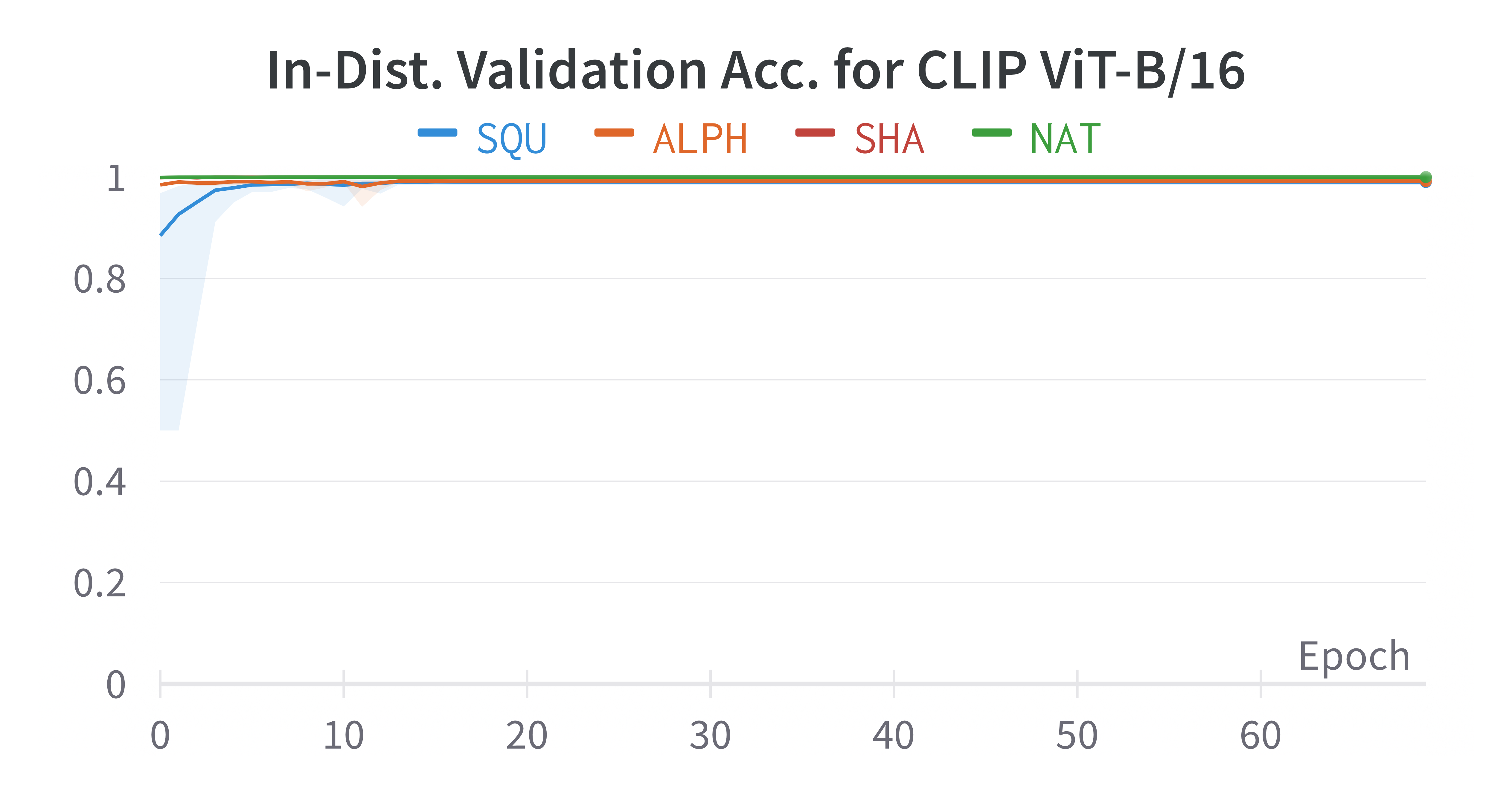
(d)

Figure 8: Average loss curves for CLIP-pretrained ResNet-50 and ViT-B/16 fine-tuned on each dataset. In-distribution generalization to color-containing datasets SHA and NAT seem much more difficult for CLIP ResNet-50 than CLIP ViT-B/16 (or any other model configuration). CLIP ViT-B/16 attains nearly 100% validation accuracy after only one epoch of fine-tuning on all datasets except SQU.

A.2 Out-of-distribution Generalization Tables

We report median test accuracy over five random seeds for each pretraining method, architecture, and fine-tuning dataset. The tables below include the four main fine-tuning datasets (SQU, ALPH, SHA, NAT; see Figure 2), the grayscale and masked versions of the SHA dataset (SHA-G and SHA-M; see Figure 4a), and grayscale and masked versions of the NAT dataset (NAT-G and NAT-M). As in Table 1, rows indicate the dataset that models are fine-tuned on, while columns indicate the test dataset. The rightmost column labeled “Avg.” is the row-wise average of accuracy scores across OOD evaluation sets (i.e. off-diagonal values), which indicates how well a model fine-tuned on a given dataset is able to generalize to other datasets. The bottom row labeled “Avg.” is the column-wise average across off-diagonal values, indicating how difficult it is for models fine-tuned on other datasets to generalize to the given dataset.

CLIP ResNet-50
	$\leftarrow$ Test $\rightarrow$
Train $\downarrow$	SQU	ALPH	SHA	SHA-G	SHA-M	NAT	NAT-G	NAT-M	Avg.
SQU	97.7	80.8	82.9	81.9	73.6	82.0	86.6	82.6	81.5
ALPH	83.5	97.4	88.9	90.1	92.9	90.7	78.2	83.8	86.9
SHA	51.3	69.3	98.1	96.2	90.8	95.2	76.3	86.6	80.8
SHA-G	65.5	80.7	98.1	98.2	95.1	93.7	95.8	91.5	88.6
SHA-M	55.9	68.1	94.7	92.1	76.1	79.6	100	86.4	82.4
NAT	53.4	76.0	95.2	96.1	96.1	97.3	87.0	94.3	85.4
NAT-G	55.6	81.3	95.4	97.3	98.0	95.7	89.7	92.7	88.0
NAT-M	59.8	80.6	90.6	91.4	90.1	94.8	94.3	95.0	85.9
Avg.	60.7	76.7	92.3	92.2	90.9	90.2	88.3	88.2

Table 3: OOD test accuracy for CLIP ResNet-50 models fine-tuned on each dataset. The model fine-tuned on NAT-G exhibits the strongest OOD generalization.

CLIP ViT-B/16
	$\leftarrow$ Test $\rightarrow$
Train $\downarrow$	SQU	ALPH	SHA	SHA-G	SHA-M	NAT	NAT-G	NAT-M	Avg.
SQU	99.5	97.7	99.1	98.9	94.8	95.5	95.0	98.1	97.0
ALPH	59.5	99.4	99.9	99.9	98.8	99.7	95.1	97.5	92.9
SHA	50.0	56.0	100	98.6	98.2	100	60.6	77.7	77.3
SHA-G	50.2	63.5	100	99.9	99.9	100	85.5	95.6	85.0
SHA-M	55.6	93.3	100	100	99.8	100	100	97.8	92.4
NAT	50.0	68.4	99.8	97.8	99.3	100	63.0	83.7	80.3
NAT-G	50.2	70.6	99.9	98.9	100	100	71.5	93.9	87.6
NAT-M	60.2	92.7	100	99.9	100	100	94.3	98.5	92.4
Avg.	53.7	77.5	99.8	99.1	98.7	99.3	84.8	92.0

Table 4: OOD test accuracy for CLIP ViT-B/16 models fine-tuned on each dataset. It is interesting to note the different patterns of generalization between models fine-tuned on SHA, SHA-G, and SHA-M. Models fine-tuned on the SHA dataset (which contains color and texture) do not generalize very well to NAT-G and NAT-M datasets; models fine-tuned on SHA-G (which removes color) generalize somewhat better to NAT-G and NAT-M; and models fine-tuned on SHA-M (which removes color and texture) attain 100% or near 100% accuracy on NAT-G and NAT-M. The same pattern holds for models fine-tuned on NAT, NAT-G, and NAT-M tasks.

ImageNet ResNet-50
	$\leftarrow$ Test $\rightarrow$
Train $\downarrow$	SQU	ALPH	SHA	SHA-G	SHA-M	NAT	NAT-G	NAT-M	Avg.
SQU	84.8	57.4	59.3	52.6	65.1	62.9	50.2	60.8	58.3
ALPH	61.3	83.7	60.4	69.0	78.5	70.2	68.0	73.9	68.8
SHA	51.2	66.7	94.4	90.1	78.4	84.0	64.1	66.5	71.6
SHA-G	53.9	72.6	70.8	94.6	84.2	74.2	90.1	78.9	75.0
SHA-M	56.2	68.9	73.7	92.4	79.4	68.7	99.3	79.8	77.0
NAT	50.3	58.3	80.4	69.5	78.6	90.5	62.4	70.7	67.2
NAT-G	50.8	72.2	70.0	82.8	89.8	78.2	69.1	81.1	75.0
NAT-M	50.1	74.9	66.9	76.2	84.0	74.2	78.9	88.4	72.2
Avg.	53.4	67.3	68.8	76.1	79.8	73.2	73.3	73.1

Table 5: OOD test accuracy for ImageNet ResNet-50 models fine-tuned on each dataset. Unlike CLIP-pretrained models, ImageNet ResNet-50 fine-tuned on SQU actually exhibits the weakest OOD generalization.

ImageNet ViT-B/16
	$\leftarrow$ Test $\rightarrow$
Train $\downarrow$	SQU	ALPH	SHA	SHA-G	SHA-M	NAT	NAT-G	NAT-M	Avg.
SQU	95.4	65.8	57.6	53.3	59.7	60.5	51.8	66.3	59.3
ALPH	81.7	97.0	50.5	51.0	59.1	52.1	52.1	67.0	59.1
SHA	50.0	50.1	100	96.2	99.3	99.4	55.8	82.5	76.2
SHA-G	50.0	61.2	100	99.8	99.8	99.9	73.9	84.8	81.4
SHA-M	57.7	88.0	99.9	99.8	99.6	97.5	99.9	97.1	91.4
NAT	50.0	50.4	97.3	80.4	97.8	100	50.4	71.8	71.2
NAT-G	50.0	50.2	98.3	91.7	99.7	99.9	54.0	87.8	82.5
NAT-M	52.2	72.3	99.8	99.3	99.9	100	91.7	98.4	87.9
Avg.	55.9	62.6	86.2	81.7	87.9	87.1	68.0	79.6

Table 6: OOD test accuracy for ImageNet ViT-B/16 models fine-tuned on each dataset. Interestingly, models fine-tuned on SHA exhibit strong generalization to the grayscale and masked versions of that dataset (but still don’t generalize to SQU or ALPH).

Randomly Initialized ResNet-50
	$\leftarrow$ Test $\rightarrow$
Train $\downarrow$	SQU	ALPH	SHA	SHA-G	SHA-M	NAT	NAT-G	NAT-M	Avg.
SQU	49.8	49.7	49.5	48.2	49.1	48.3	49.6	50.0	49.2
ALPH	53.1	69.2	58.9	59.0	55.2	58.6	50.0	50.4	55.0
SHA	51.2	69.3	82.6	80.4	82.3	82.9	53.8	61.8	68.8
SHA-G	50.6	67.2	85.0	85.5	87.5	84.0	59.8	67.4	71.6
SHA-M	50.0	57.0	77.3	77.0	77.0	75.0	78.3	74.3	69.9
NAT	52.9	69.5	81.6	80.4	80.3	80.2	55.4	68.0	69.7
NAT-G	51.1	64.2	77.3	83.6	82.8	82.5	61.3	72.5	73.4
NAT-M	50.0	59.4	77.2	79.1	80.3	79.2	69.2	74.4	70.6
Avg.	51.3	62.3	72.4	72.5	73.9	72.9	59.5	63.5

Table 7: OOD test accuracy for randomly-initialized ResNet-50 models trained on each dataset. Models attain surprisingly high in-distribution test accuracy for certain datasets, such as SHA and SHA-G. Models trained on SQU appear to learn nothing even though their loss curves diminish (see Figure 6). This indicates that models are memorizing training examples, which is consistent with results from prior work (e.g. Kim et al. (2018)).

Randomly Initialized ViT-B/16
	$\leftarrow$ Test $\rightarrow$
Train $\downarrow$	SQU	ALPH	SHA	SHA-G	SHA-M	NAT	NAT-G	NAT-M	Avg.
SQU	51.7	51.8	51.0	53.5	52.7	53.8	51.4	53.9	52.6
ALPH	49.9	54.8	51.7	51.9	56.8	52.0	49.9	51.4	51.9
SHA	50.0	50.1	92.9	66.2	62.6	73.8	50.7	56.0	58.5
SHA-G	50.0	50.5	74.2	78.8	66.5	66.4	55.7	56.4	60.0
SHA-M	50.0	50.0	56.5	59.6	53.5	55.5	81.3	63.5	59.5
NAT	50.1	51.7	75.7	58.7	62.2	76.7	53.4	62.8	59.2
NAT-G	50.2	51.8	64.1	69.9	70.7	67.0	55.9	65.9	62.8
NAT-M	50.0	50.5	56.4	56.8	58.4	58.2	55.0	66.2	55.0
Avg.	50.0	50.9	61.4	59.5	61.4	61.0	56.8	58.6

Table 8: OOD test accuracy for randomly-initialized ViT-B/16 models trained on each dataset. Somehwat surprisingly given their larger receptive field size, randomly initialized ViTs perform worse overall than randomly initialized ResNets (Table 7).

A.3 Area Under the ROC Curve for CLIP Models

In addition to reporting median test accuracy across seeds, we report median area under the ROC curve for CLIP ResNet-50 and CLIP ViT-B/16. Table 9 below mirrors Table 1 from the main paper.

CLIP ResNet-50
	$\leftarrow$ Test $\rightarrow$
Train $\downarrow$	SQU	ALPH	SHA	NAT	Avg.
SQU	0.99	0.95	0.93	0.86	0.91
ALPH	0.96	0.99	0.96	0.97	0.96
SHA	0.8	0.91	1.0	0.99	0.9
NAT	0.83	0.94	0.99	0.99	0.92
Avg.	0.86	0.93	0.96	0.94

CLIP ViT-B/16
	$\leftarrow$ Test $\rightarrow$
Train $\downarrow$	SQU	ALPH	SHA	NAT	Avg.
SQU	1.00	1.00	1.00	1.00	1.00
ALPH	0.93	1.00	1.00	1.00	0.98
SHA	0.62	0.91	1.00	1.00	0.84
NAT	0.63	0.93	1.00	1.00	0.85
Avg.	0.73	0.95	1.00	1.00

Table 9: Out-of-distribution test AUC for CLIP models fine-tuned on each dataset. Rows indicate the dataset that models are fine-tuned on, while columns indicate the test dataset. Each cell is the median performance over five random seeds. The rightmost column labeled “Avg.” is the row-wise average of accuracy scores across OOD evaluation sets (i.e. off-diagonal values), which indicates how well a model fine-tuned on a given dataset is able to generalize to other datasets. The bottom row labeled “Avg.” is the column-wise average across off-diagonal values, indicating how difficult it is for models fine-tuned on other datasets to generalize to the given dataset.

Models fine-tuned on the Shapes and Naturalistic datasets attain rather high AUC across all OOD test datasets, notably including the Alphanumeric task (which does not contain color or texture). CLIP ResNet-50 in particular attains $>0.8$ AUC across all fine-tuning conditions and test datasets. This is in contrast to median accuracy results reported in Table 1, which shows more of a dramatic “upper triangular” pattern. This indicates that some of the models that achieve poor OOD test accuracy may perform much more strongly with a correctly calibrated bias. Even still, the “upper triangular” pattern is still evident here—models fine-tuned on Squiggles and Alphanumeric tasks demonstrate stronger generalization than models fine-tuned on Shapes and Naturalistic tasks. Furthermore, ViT still outperforms ResNet, achieving perfect AUC across all test datasets when fine-tuned on Squiggles.

A.4 Testing Models on Evaluation Sets from Puebla & Bowers (2022)

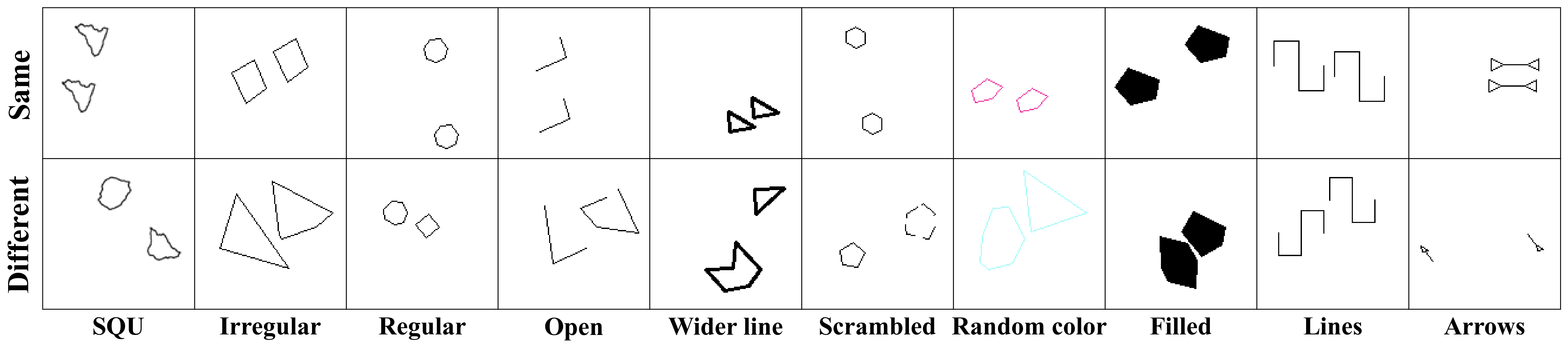
Figure 9: Examples of “same” and “different” stimuli from all 10 evaluation sets in Figure 10. The first dataset (SQU) is the in-distribution test set and is the same as our SQU dataset from the main body of this paper. The other nine datasets are generated following Puebla & Bowers (2022).

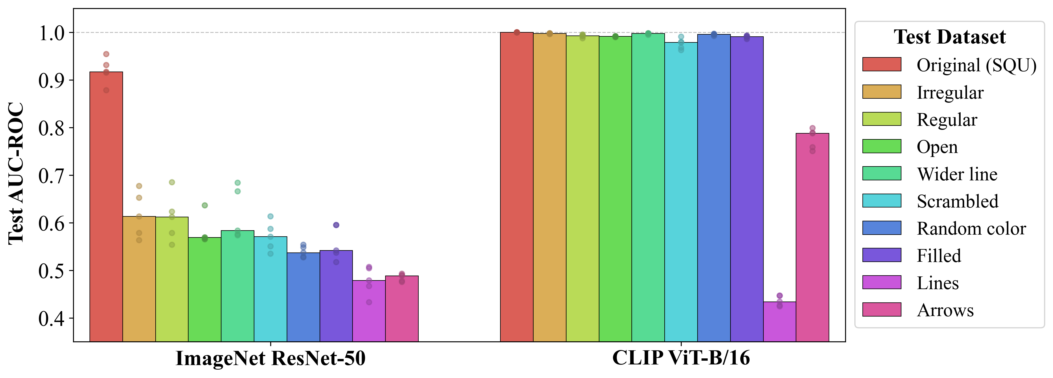
Figure 10: Out-of-distribution test AUC-ROC for ImageNet ResNet-50 and CLIP ViT-B/16 fine-tuned on Squiggles. Median AUC-ROC over five seeds is reported with individual runs also shown. The legend on the right indicates the test dataset. The two red bars in this figure show in-distribution test AUC-ROC, which is also reported for CLIP ViT-B/16 in Table 9.

We test two of our models on the evaluation sets from Puebla & Bowers (2022): ImageNet ResNet-50 fine-tuned on SQU, which is roughly equivalent to the models tested in Puebla & Bowers (2022), and CLIP ViT-B/16 fine-tuned on SQU, which is our best model. We use code from Puebla & Bowers (2022) to generate test sets of $6,400$ images evenly split between the classes, which is equal to the size of our test sets. Figure 9 show all 10 evaluation datasets used in this section. Furthermore, we report median AUC-ROC to better match Puebla & Bowers (2022), who report mean AUC-ROC. The rest of our methodology follows Section 2.

Our ImageNet ResNet-50 results are comparable to results from Puebla & Bowers (2022) but not identical. Differences in our specific results may be due to our differing methods for creating our datasets. For example, the sizes of their objects are variable and may either be smaller or larger than our chosen size of $64x64$ pixels (see Figure 9 for examples). Their ImageNet ResNet-50 model is fine-tuned on Fleuret et al. (2011) stimuli in which the sizes of the objects also vary, whereas our model is fine-tuned on objects of a fixed size. We also thicken the lines of our SQU stimuli, while Puebla & Bowers (2022) do not. Furthermore, they use more fine-tuning images than us (28,000 versus 6,400), and their hyperparameters likely differ as well. Even still, the larger pattern of results is the same—ImageNet ResNet-50 fine-tuned on the same-different relation using stimuli from Fleuret et al. (2011) (our SQU stimuli) attains relatively high in-distribution test accuracy but struggles to generalize out-of-distribution. This agrees with the results we obtain using our evaluation sets (SQU, ALPH, SHA, & NAT); Table 5 shows that ImageNet-ResNet-50 fine-tuned on SQU struggles to generalize out-of-distribution.

In contrast, CLIP ViT-B/16 fine-tuned on our Squiggles dataset achieves perfect or nearly perfect in- and out-of-distribution generalization, with the exception of two test datasets (Lines and Arrows). This performance is rather remarkable given that objects in the evaluation datasets from Puebla & Bowers (2022) vary greatly in size, whereas our CLIP ViT-B/16 model is fine-tuned on objects of a fixed size only. This suggests that CLIP ViT-B/16 fine-tuned on SQU may learn a same-different relation that is invariant to certain qualities (such as object size) without explicit fine-tuning for such invariance. Figure 11 shows examples of stimuli from the two more challenging datasets (Lines and Arrows) for which all five CLIP ViT-B/16 random seeds make errors. For Arrows, this lack of generalization may be due to symbols overlapping or being much closer to each other than any stimuli in our fine-tuning data. Failure on this dataset may simply be due to difficulties in segmenting the objects rather than a lack of a general same-different representation. We also see a very slight decrease in test AUC-ROC for the Scrambled dataset, which is an interesting case. Errors made for this dataset were primarily due to our model misclassifying slightly scrambled and unmodified polygons as the “same.” This error may offer insight into how exactly CLIP ViT-B/16 fine-tuned on Squiggles compares objects in an image.

However, the most surprising finding is that CLIP ViT-B/16 classifies all stimuli in the Lines dataset as “same” (see Appendix D), and that its ROC-AUC score is below $0.5$. This is striking because all objects in the Lines dataset are actually the same under reflection. This result makes it very tempting to conclude that CLIP ViT-B/16 actually learns to generalize to reflections without ever being fine-tuned to do so, although further work is necessary to draw this conclusion with any certainty. Furthermore, if models see the same image multiple times but flipped horizontally during pretraining, which is a common data augmentation, then pretrained models may already have reflection invariance baked in. Pretraining data augmentations have been shown to have such an effect on other abstract relational learning tasks (Davidson et al., 2023). Finally, the Lines dataset consists entirely of one unique object that is scaled and flipped to create all stimuli, so if our model makes an error for this particular object, that error could plausibly occur across the entire dataset.

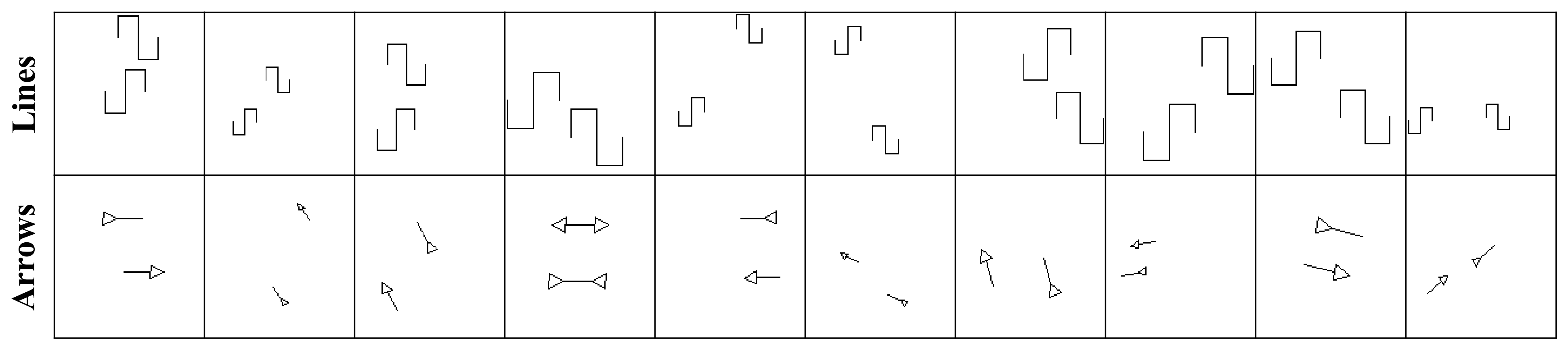
Figure 11: “Different” images misclassified by CLIP ViT-B/16 as “same” from Puebla & Bowers (2022)’s Lines and Arrows datasets. These stimuli are randomly sampled from the set of stimuli misclassified by all five seeds. Nearly $100\%$ of model errors across evaluation datasets and seeds are mistaking “different” stimuli for “same” stimuli, so we only show mistakes of this kind. Note that the “different” Lines stimuli (middle row) are actually the same under reflection. Confusion matrices computed on these two datasets for the models tested in this section can be found in Appendix D.

A.5 Probing CLIP Embeddings

In order to determine the degree to which CLIP pretraining alone encodes useful information for learning the same-different relation, we perform a linear probe on the CLIP ResNet-50 and CLIP ViT-B/16 models. As in our main experiments, we append a linear binary classifier to the visual backbone of each model. However, in this experiment, we freeze the pretrained weights in the backbone of each model and train only the parameters of the classifier on the fixed embeddings given by the backbone. Results are displayed in Table 10.

CLIP ResNet-50 Probe
	$\leftarrow$ Test $\rightarrow$
Train $\downarrow$	SQU	ALPH	SHA	NAT	Avg.
SQU	62.4	50.0	50.0	50.0	50.0
ALPH	50.0	72.7	50.1	49.8	49.9
SHA	50.0	50.0	85.6	50.3	50.1
NAT	50.0	49.9	52.5	85.6	50.8
Avg.	50.0	50.0	50.8	50.0

CLIP ViT-B/16 Probe
	$\leftarrow$ Test $\rightarrow$
Train $\downarrow$	SQU	ALPH	SHA	NAT	Avg.
SQU	81.9	51.1	55.8	52.7	53.2
ALPH	50.0	94.4	53.1	58.5	53.9
SHA	50.0	50.0	99.9	90.4	63.5
NAT	50.0	50.1	70.6	100	56.9
Avg.	50.0	50.4	59.8	67.2

Table 10: Out-of-distribution test accuracy for the best linear probe trained on CLIP embeddings of each dataset.

We find that the linear probe can generally exhibit rather high in-distribution generalization. CLIP embeddings of Naturalistic stimuli produce the highest in-distribution test accuracy, followed closely by Shapes. CLIP embeddings of Alphanumeric and Squiggles datasets are more difficult to learn from. This mirrors the ordering observed in Section 3.2 in which the two same-different tasks containing color and texture features tend to be easier to learn, while the shape-based tasks tend to be more difficult. The fact that Alphanumeric and Squiggles probes are unable to generalize OOD, however, is odd considering the fact that the solutions to both of these datasets should be the same (based on shape); this implies there is some other signal that linear probes are picking up on in order to separate “same” and “different” stimuli in these cases.

In the case of CLIP ResNet-50, the linear probe does not generalize to any OOD stimuli. On the other hand, CLIP ViT-B/16 probes trained on Shapes or Naturalistic stimuli generalize somewhat well to each other ($90.4\%$ generalization from Shapes to Naturalistic; $70.6\%$ from Naturalistic to Shapes). Somewhat surprisingly, the CLIP ViT-B/16 probe trained on the Squiggles dataset does not generalize the relation to other datasets despite the impressive generalization performance of the fully fine-tuned model.

A.6 CLIP Embedding Cosine Similarity Distributions

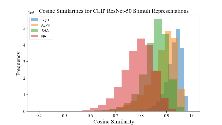
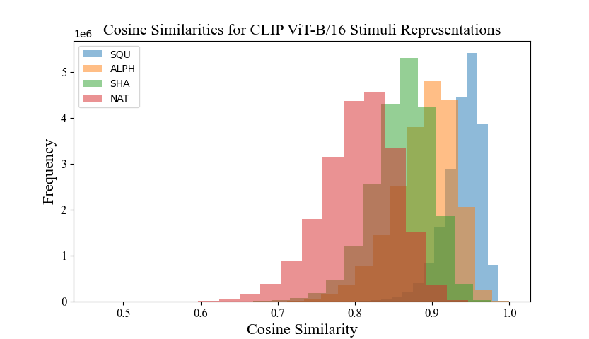
Figure 12: Distribution of cosine similarities between CLIP ResNet-50 representations of the Squiggles, Alphanumeric, Shapes, and Naturalistic datasets. These cosine similarities are calculated before fine-tuning. $n=6,400$ for each dataset, 20.48M pairs calculated per dataset.

Figure 13: Distribution of cosine similarities between CLIP ViT-B/16 representations of the Squiggles, Alphanumeric, Shapes, and Naturalistic datasets. These cosine similarities are calculated before fine-tuning. $n=6,400$ for each dataset, 20.48M pairs calculated per dataset.

	Before Fine-tuning		Fine-tuned on SQU
Dataset $\downarrow$	ResNet-50	ViT-B/16	ResNet-50	ViT-B/16
noise	0.992	0.993	0.983	0.997
SQU	0.929	0.940	0.992	0.283
ALPH	0.881	0.889	0.984	0.634
SHA	0.855	0.861	0.949	0.548
NAT	0.788	0.805	0.937	0.568

Table 11: Average pairwise cosine similarity between CLIP embeddings of training stimuli within each dataset. Because $n=6,400$ for each dataset, averages are computed over 20.48M pairs. We extract CLIP embeddings before fine-tuning on the same-different task and after fine-tuning on the Squiggles task (median across five seeds).

Interestingly, Table 11 shows that ViT-B/16’s embeddings seem to become more distinct during fine-tuning whereas ResNet-50’s become closer together. This is likely not due to differences in generalization performance given that the median difference between ViT-B/16 and ResNet-50 for within-distribution generalization is only $1.9\%$, and the median difference in out-of-distribution generalization is $13.9\%$. We do not have a clear explanation for this phenomenon, and also concede that it may be a methodological problem resulting from calculating cosine similarity between CLIP embeddings after extensive fine-tuning.

A.7 Fine-tuning on Noise

We initially calculated average pairwise cosine similarity for CLIP representations of random Gaussian noise as a baseline for measuring visual diversity within our datasets (Table 2). However, after observing a pattern in which more closely-embedded datasets induce stronger out-of-distribution generalization, we decided to see whether models perform even better when they are fine-tuned on a version of the same-different task where they must label two same-versus-different 64x64 squares of random Gaussian noise (see Figure 14). Theoretically, if models fine-tuned on this task are forced to compare objects on the level of individual pixels, they should be able to generalize to any same-different dataset in which objects are the same on a pixel level (the definition of sameness we employ in this work).

 

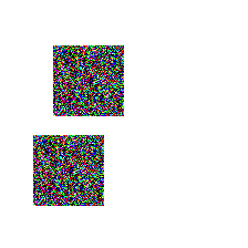
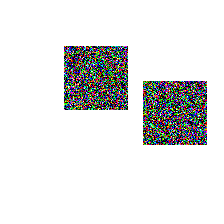
Figure 14: Examples of stimuli used when fine-tuning on noise. From left to right: a single example object; a stimulus labeled as “same;” a stimulus labeled as “different.” All noise stimuli were sampled from a Gaussian distribution with $\mu=0$ and $\sigma=1$.

We use the same methodology as described in Section 2. That is, we fine-tune CLIP ResNet-50 and CLIP ViT-B/16 on this task, sweeping over the learning rates (1e-4, 1e-5, 1e-6, 1e-7, 1e-8) and two learning rate schedulers (exponential, ReduceLROnPlateau). We report results for the best models trained for 70 epochs with a batch size of 128 in Table 12.

	$\leftarrow$ Test $\rightarrow$
Model $\downarrow$	NOISE	SQU	ALPH	SHA	NAT	Avg.
ViT-B/16	95.3	50.3	65.1	97.1	96.9	77.4
ResNet-50	94.9	50	50	61.2	59.3	55.1
Avg.	95.1	50.2	57.6	79.2	78.1

Table 12: Out-of-distribution test accuracy for CLIP models fine-tuned on noise. Rows indicate model architecture and number of epochs, while columns indicate the test dataset. Each cell is the median performance over five random seeds. The rightmost column labeled “Avg.” is the row-wise average of accuracy scores across OOD evaluation sets (i.e. not including the NOISE column), which indicates how well a model is able to generalize to other datasets. The bottom row labeled “Avg.” is the column-wise average, indicating how difficult it is for models fine-tuned on noise to generalize to that given dataset.

As shown in Table 12, models fine-tuned on noise largely fail to generalize. One likely explanation for this lack of generalization is that models fine-tuned on noise learn to attend to small regions in both objects (e.g. two adjacent pixels in the corner of each object) and calculate whether those small regions are equivalent. This might help explain why CLIP ViT-B/16 fine-tuned on noise generalizes quite strongly to the SHA and NAT datasets—these two datasets contain textures, so this potential strategy of computing equality based on highly localized features would work well. On the other hand, this strategy would likely fail for stimuli in the Squiggles and Alphanumeric tasks, which consist of primarily empty space and require the integration of more global shape information. Although the idea of training on noise for abstract-relations is promising in theory (since there should not be spurious, non-generalizing visual features), it would require careful design to counteract such undesirable local “shortcuts” (Geirhos et al., 2020).

A.8 Sensitivity of OOD Generalization to Random Seed

In Table 1, we report median out-of-distribution test accuracy across five random seeds for CLIP ResNet-50 and CLIP ViT-B/16. Here, we extend this table by reporting out-of-distribution test accuracy for all five random seeds.

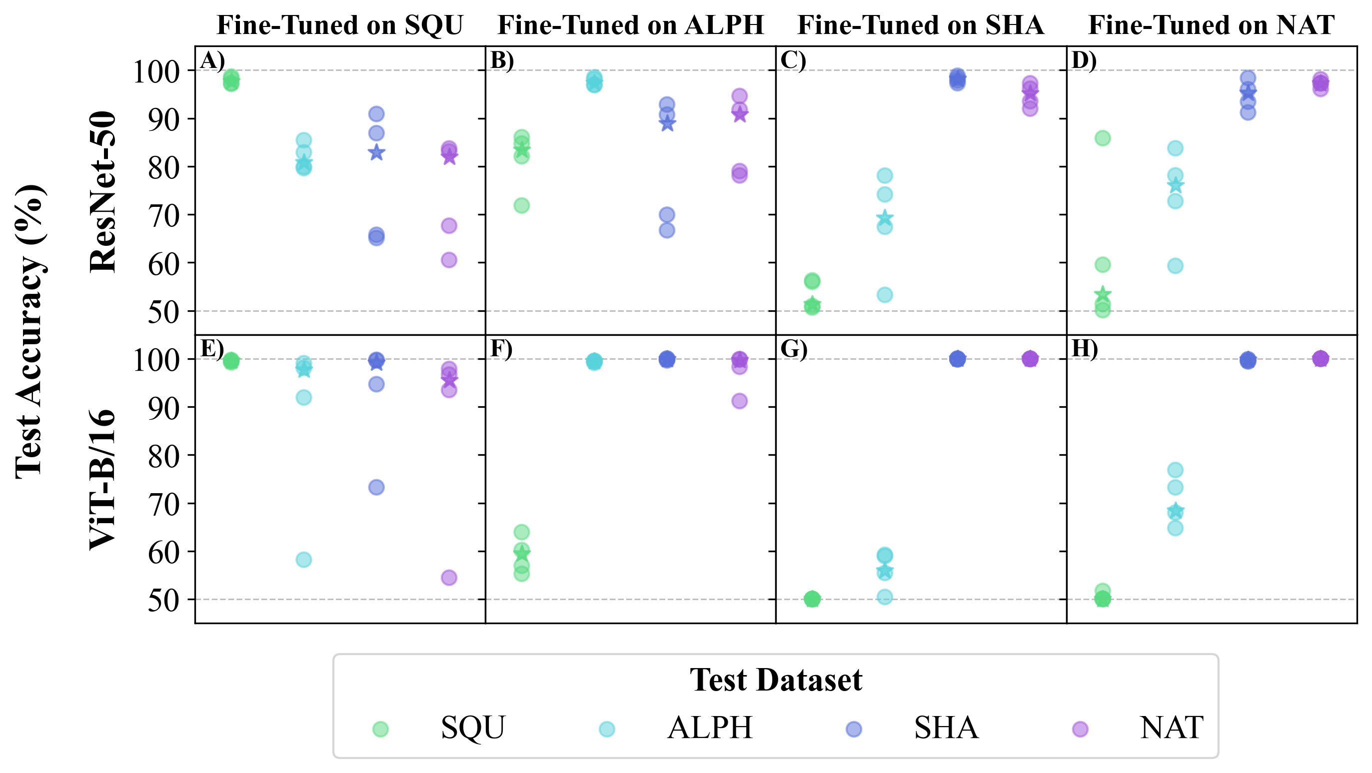
Figure 15: Out-of-distribution test accuracy for CLIP models for each fine-tuning dataset across all five random seeds. The top row shows test accuracy for CLIP ResNet-50, while the bottom row shows test accuracy for CLIP ViT-B/16. The columns indicate the fine-tuning dataset (from left to right: SQU, ALPH, SHA, & NAT), while the legend indicates the test dataset. Each individual plot point is the test accuracy for a given random seed. Stars represent the median test accuracy, which are equivalent to the values reported in Table 1.

All model configurations demonstrate some sensitivity to random seed. However, the two best generalizing models—CLIP ResNet-50 fine-tuned on ALPH (Figure 15B) and CLIP ViT-B/16 fine-tuned on SQU (Figure 15E)—demonstrate a distinct bimodal distribution across seeds. While some seeds attain high test accuracy across all three OOD test sets, one (CLIP ViT) or two seeds (CLIP ResNet) perform substantially worse across all three sets. This creates a visible gap between points that persists across all three OOD test sets in panels B and E in Figure 15. Other configurations demonstrate such a gap for one or two test sets (e.g. panel A and panel D in Figure 15), but no other configurations demonstrate such a gap for all three OOD sets.

It is interesting to consider the fact that the only randomness in our setup for these models is in the data batching (since models are initialized with deterministic, pretrained weights). This indicates that the order in which models see particular examples from the training set is important for abstraction and determines whether or not models discover the generalizing solution.

Appendix B Inductive Bias Experiment Details

B.1 Grayscale and Mask Details

Grayscaled Shapes. Images were taken from the Shapes dataset (Section 2) and converted to grayscale using the PIL ImageOps.grayscale method.

Masked Shapes. Images were taken from the Shapes dataset. Because the background was already white, we selected RGB pixels that were $\leq$ (250, 250, 250) and replaced them with pixels of the value (100, 100, 100). Extra pixels with any values greater than 250 that are not equal to the background color (255, 255, 255) were also converted to (100, 100, 100).

Because training datasets are constructed by sampling random objects, the exact objects used between the original, grayscale, and masked datasets are not the same.

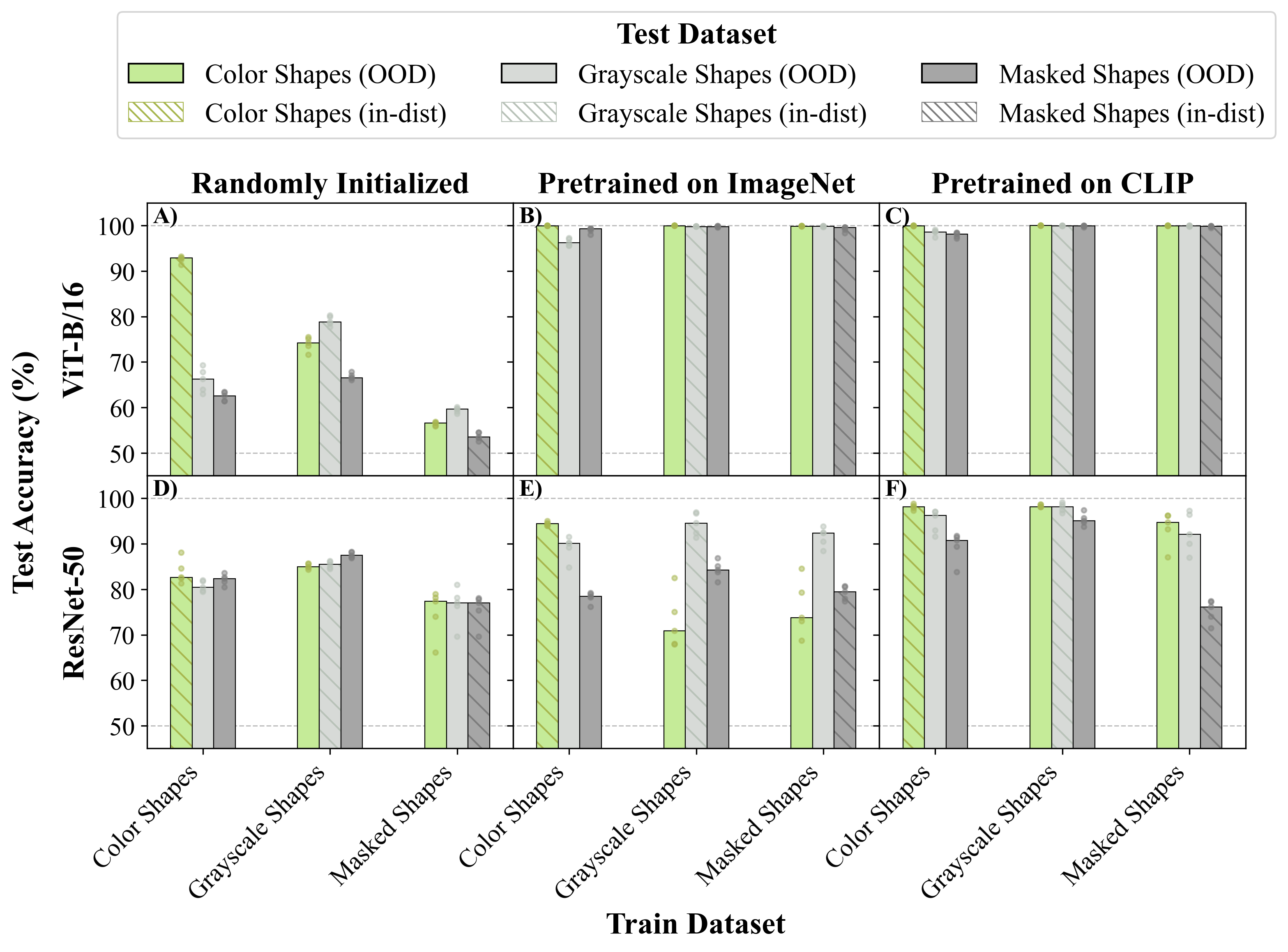
Figure 16: Test accuracy for models trained or fine-tuned on one version of the Shapes dataset (Color, Grayscale, Masked) and then tested on all three versions of the dataset. Example stimuli shown in Figure 4a. Hatched bars indicate in-distribution accuracy. Median results for the same hyperparameters trained for five different seeds are reported, with individual runs also plotted as translucent points.

B.2 Dissociating Color, Texture, and Shape

Results from Figure 5 suggest that some models learn to rely on certain features more than others to differentiate between objects in an image. To delve deeper into this result, we create a series of eight testing datasets based on the Shapes dataset where we vary whether shape, color, and texture are the same or different between two objects in an image (examples in Figure 17). We label each set of images with a string of letters representing whether color (C), texture (T), or shape (S) are the same. For example, images containing two objects that are the same color, different textures, and the same shape are labeled CS. CTS and “none” represent the tokens being completely the same or completely different respectively. We then evaluate the same models from Figure 5 on each of these test sets by measuring the proportion of “same” predictions for each dataset. If this proportion is high, the model views stimuli in those datasets as “same”; if this proportion is low, it means that the model views them as “different.” The first few rows of Table 13 show the hypothesized behavior of theoretical models with certain inductive biases when tested on each of the generated datasets. If a model is making predictions by comparing object shape (for example), then it should predict “same” whenever the shape of the two objects in an image are the same (S) and “different” otherwise. Ideally, a model that has picked up on our definition of “same” as pixel-level similarity should not be predicting “same” for any case except for CTS.

	Acc.	Proportion of “Same” Predictions
Predicted $\downarrow$	acc.	none	S	T	TS	C	CS	CT	CTS
(no bias)	1.00	0.00	0.00	0.00	0.00	0.00	0.00	0.00	1.00
color	1.00	0.00	0.00	0.00	0.00	1.00	1.00	1.00	1.00
texture	1.00	0.00	0.00	1.00	1.00	0.00	0.00	1.00	1.00
shape	1.00	0.00	1.00	0.00	1.00	0.00	1.00	0.00	1.00
ViT-B/16 (Rand) $\downarrow$	acc.	none	S	T	TS	C	CS	CT	CTS
Color Shapes	0.91	0.15	0.15	0.17	0.16	0.86	0.87	0.96	0.97
ViT-B/16 (CLIP) $\downarrow$	acc.	none	S	T	TS	C	CS	CT	CTS
Color Shapes	1.00	0.00	0.01	0.03	0.09	0.12	0.41	0.89	1.00
Grayscale Shapes	1.00	0.00	0.00	0.01	0.06	0.02	0.26	0.59	1.00
Masked Shapes	1.00	0.00	0.04	0.00	0.24	0.00	0.47	0.02	1.00

Table 13: Predicted results of dissociation experiments compared to actual results from ViT-B/16 models fine-tuned on different versions of the original SHA dataset. The proportion of “same” predictions for different types of images should change based on the inductive bias a given model is using. Even CLIP-pretrained ViT-B/16, which seemed from Figure 5 to be unbiased, is revealed to have a slight bias towards either color+texture or shape depending on its fine-tuning dataset. Median results over five seeds are reported for each row. Results for Random ViT-B/16 fine-tuned on Grayscale and Masked Shapes are not shown due to low accuracy (making the results difficult to interpret); full table is Table 14.

Comparing the first row of results to predicted behavior, we immediately see that the “same” predictions made by Random ViT-B/16 on the Color Shapes dataset pattern closely with our predicted “color-biased model” behavior. This confirms our result from Figure 5, which showed that this model could not generalize to datasets without color. If the same architecture is pretrained with CLIP and then fine-tuned on the Color Shapes dataset, its predictions become much more sensitive to texture and shape. Upon closer inspection, however, these results still reveal a residual bias towards color and texture that was not as apparent in Figure 5. For example, when models are tested on objects with the same color and texture but different shapes (CT), CLIP ViT-B/16 will classify them as the same when fine-tuned on Color or Grayscale Shapes, but different when fine-tuned on Masked Shapes. This indicates that CLIP ViT-B/16 still has an inductive bias towards color and texture after pretraining, and only resorts to comparing object shape if there are no other features available in its fine-tuning data. Results in the full table for all models tell a similar story (Table 14): even models that generalize well OOD exhibit specific, understandable biases determined by features available in their training datasets.

One limitation with this approach is that the difference between color and texture is somewhat ill-defined on a pixel level. This may be an explanation for the fact that no models tested exhibited a pattern close to our hypothesized “texture” model, despite evidence for “color” and “shape” being quite clear.

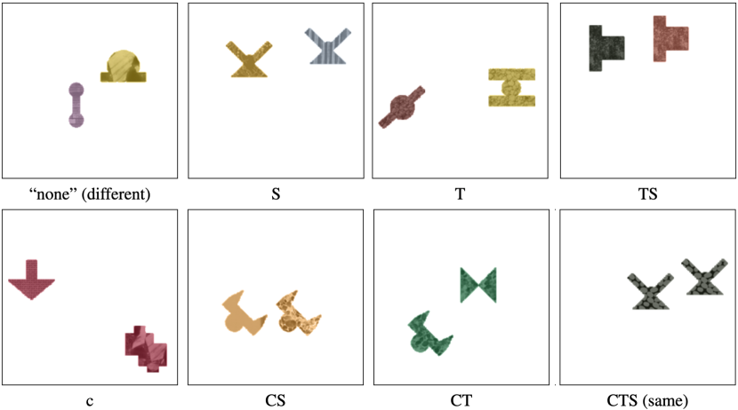
Figure 17: Examples of training images from every Table 13 and Table 14 testing dataset. Every test dataset contained 6400 images and 300 unique objects.

	Acc.	Proportion of “Same” Predictions
Predicted $\downarrow$	acc.	none	S	T	TS	C	CS	CT	CTS
(no bias)	1.00	0.00	0.00	0.00	0.00	0.00	0.00	0.00	1.00
color	1.00	0.00	0.00	0.00	0.00	1.00	1.00	1.00	1.00
texture	1.00	0.00	0.00	1.00	1.00	0.00	0.00	1.00	1.00
shape	1.00	0.00	1.00	0.00	1.00	0.00	1.00	0.00	1.00
ViT-B/16 $\downarrow$	acc.	none	S	T	TS	C	CS	CT	CTS
SHA (Rand)	0.91	0.15	0.15	0.17	0.16	0.86	0.87	0.96	0.97
GRAY-SHA (Rand)	0.77	0.33	0.35	0.45	0.50	0.41	0.48	0.80	0.87
MASK-SHA (Rand)	0.61	0.52	0.65	0.55	0.66	0.59	0.68	0.63	0.73
SHA (ImageNet)	1.00	0.00	0.02	0.01	0.06	0.34	0.81	0.82	1.00
GRAY-SHA (ImageNet)	1.00	0.00	0.01	0.00	0.06	0.05	0.40	0.47	1.00
MASK-SHA (ImageNet)	1.00	0.00	0.15	0.00	0.28	0.00	0.82	0.03	1.00
SHA (CLIP)	1.00	0.00	0.01	0.03	0.09	0.12	0.41	0.89	1.00
GRAY-SHA (CLIP)	1.00	0.00	0.00	0.01	0.06	0.02	0.26	0.59	1.00
MASK-SHA (CLIP)	1.00	0.00	0.04	0.00	0.24	0.00	0.47	0.02	1.00
ResNet-50 $\downarrow$	acc.	none	S	T	TS	C	CS	CT	CTS
SHA (Rand)	0.83	0.25	0.29	0.34	0.35	0.43	0.44	0.71	0.90
GRAY-SHA (Rand)	0.84	0.27	0.29	0.39	0.41	0.38	0.40	0.81	0.96
MASK-SHA (R)	0.79	0.26	0.36	0.37	0.48	0.34	0.47	0.47	0.85
SHA (ImageNet)	0.93	0.15	0.49	0.17	0.59	0.39	0.94	0.43	1.00
GRAY-SHA (ImageNet)	0.79	0.41	0.64	0.44	0.65	0.59	0.96	0.61	0.99
MASK-SHA (ImageNet)	0.84	0.17	0.49	0.17	0.45	0.27	0.83	0.28	0.85
SHA (CLIP)	0.98	0.04	0.11	0.05	0.15	0.20	0.60	0.47	1.00
GRAY-SHA (CLIP)	0.98	0.04	0.42	0.07	0.54	0.06	0.53	0.15	1.00
MASK-SHA (CLIP)	0.98	0.04	0.90	0.05	0.95	0.05	0.92	0.07	1.00

Table 14: Predicted results of dissociation experiments, along with actual results from all models trained on different versions of the original Shapes dataset. Ideally, the proportion of “same” predictions for different types of images should change based on the inductive bias a given model is using. Median results over five seeds are reported for each row. SHA=Color Shapes, GRAY-SHA=Grayscale Shapes, MASK-SHA=Masked Shapes.

One insight from Table 14 not discussed in the main paper is ResNet-50’s tendency to be biased more towards shape than ViT-B/16. Considering previous work that describes ViT models as more able to attend to global features than ResNet-50 models Raghu et al. (2021), this pattern is surprising, as shape seems to be a more global feature than texture or color.

Appendix C Diversity of Training Data Heatmaps

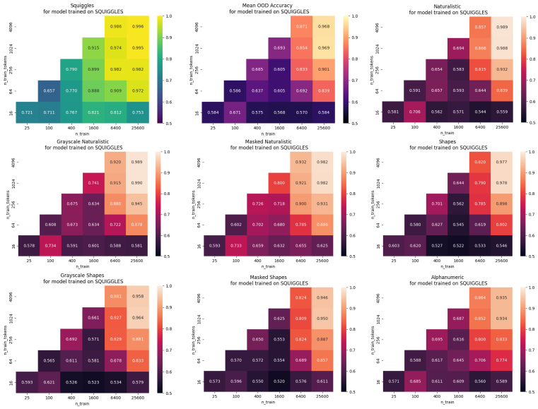
Figure 18: Validation accuracies for a ViT-B/16 ImageNet model fine-tuned on different numbers of unique objects and different amounts of Squiggles stimuli. Hyperparameters chosen correspond with the best-performing Squiggles model from 3. Each cell is averaged over five different seeds. ImageNet ViT-B/16 must be fine-tuned on at least 25,600 images containing at least 1,024 unique tokens to achieve high out-of-distribution accuracy.

Appendix D Out-of-distribution Test Confusion Matrices

We consider the pattern of errors produced by two of our models: ImageNet ResNet-50 fine-tuned on SQU, which is the most similar to models tested in some prior work (Funke et al., 2021; Puebla & Bowers, 2022), and CLIP ViT-B/16 fine-tuned on SQU, which is our best model. We compute confusion matrices for both of these models on our four main test sets (SQU, ALPH, SHA, & NAT) as well as the Lines and Arrows test sets from Puebla & Bowers (2022), which our CLIP ViT-B/16 model finds challenging (see Appendix A.4 for visual examples and results). We report matrices for the random seed that yields the median in-distribution test accuracy (i.e. the run that corresponds to the bars in Figure 3).

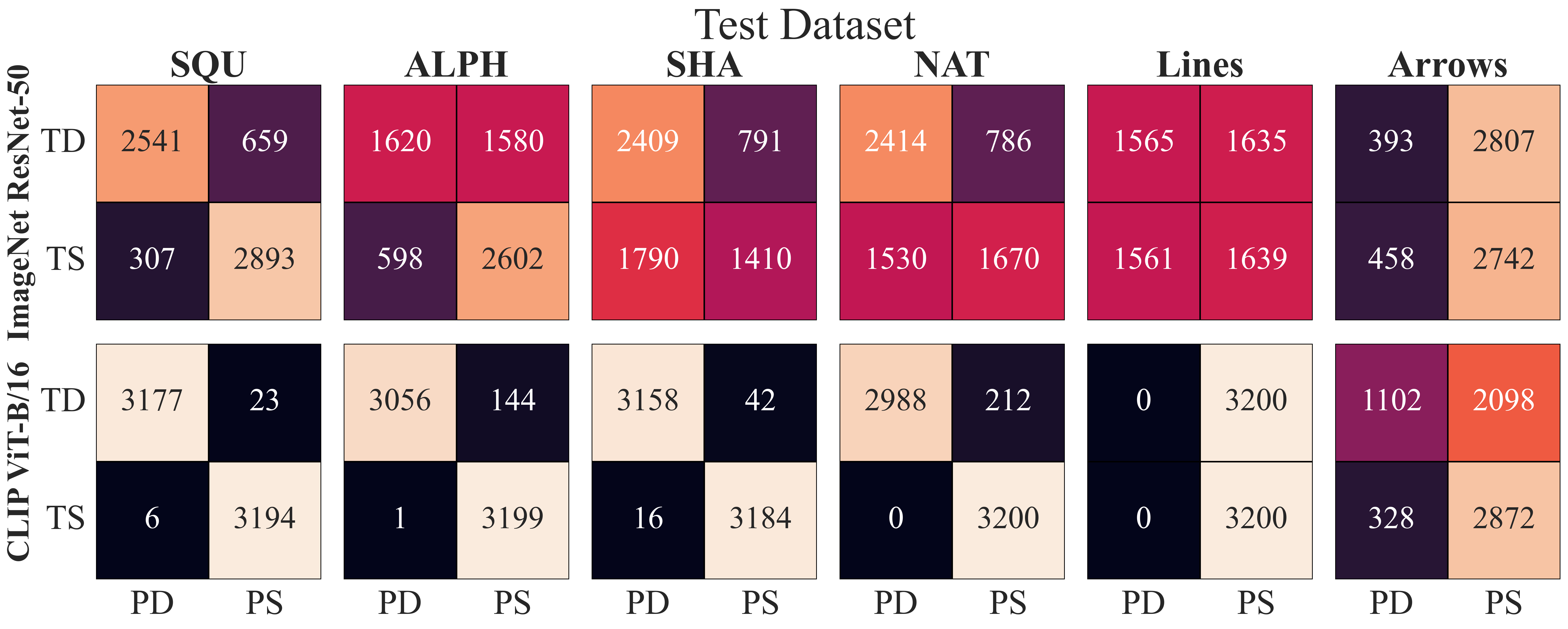
Figure 19: Confusion matrices for ImageNet ResNet-50 (top row) and CLIP ViT-B/16 (bottom row) fine-tuned on SQU. Each column gives confusion matrices for a given test set as indicated by the labels above. The rows of the confusion matrices are the true labels (TD means “true different”; TS means “true same”), while the columns of the matrices are the predicted classes (PD means “predicted different”; PS means “predicted same”). Each cell in the matrix shows the number of test images with a given true label and a predicted label as assigned by each model.

In general, both ImageNet ResNet-50 and CLIP ViT-B/16 models tend to mistake “different” stimuli for “same” stimuli more frequently than the converse. However, this is not always the case for ImageNet ResNet-50—as the top row of Figure 19 shows, ResNet makes the opposite error (mistaking “same” for “different”) much more frequently when tested on SHA and NAT datasets. This is never the case for CLIP ViT-B/16 (bottom row of Figure 19). Furthermore, the difference in frequency between the two types of errors is much more stark for CLIP ViT-B/16; the vast majority of errors made by this model across all test datasets are mistaking “different” stimuli for “same” stimuli. Hochmann (2021) argues that much of the studies on same-different relation learning in children and animals can actually be accounted for by subjects learning a concept of “same” without learning a symmetric concept of “different;” in other words, a subject can achieve high performance on many same-different tasks used in the cognitive science literature by only recognizing when two objects are the same as each other (without explicitly representing “different”). This seems to align with the errors made by CLIP ViT-B/16. It is possible that this model learns a stronger or more coherent concept of sameness and thus decides to output “same” whenever it is less certain.

Another notable result is the CLIP ViT-B/16 confusion matrix for the Lines dataset from Puebla & Bowers (2022). The model assigns the label “same” to $100\%$ of the “different” stimuli with relatively high confidence (as indicated by the $<0.5$ AUC-ROC score on this dataset in Appendix A.4). This is in contrast to ImageNet ResNet-50, which appears to assign category labels at random for the Lines dataset. As extrapolated in Appendix A.4, the “different” stimuli in this dataset are actually the same under reflection, suggesting that CLIP ViT-B/16 fine-tuned on SQU may learn a reflection-invariant same-different relation despite not being fine-tuned for such invariance (although this is speculative).

References

- Altabaa et al. (2023) Awni Altabaa, Taylor Webb, Jonathan Cohen, and John Lafferty. Abstractors: Transformer modules for symbolic message passing and relational reasoning, 2023.
- Anderson et al. (2018) Erin M Anderson, Yin-Juei Chang, Susan Hespos, and Dedre Gentner. Comparison within pairs promotes analogical abstraction in three-month-olds. Cognition, 176:74–86, 2018.
- Brady et al. (2008) Timothy F. Brady, Talia Konkle, George A. Alvarez, and Aude Oliva. Visual long-term memory has a massive storage capacity for object details. Proceedings of the National Academy of Sciences, 105(38):14325–14329, 2008. doi: 10.1073/pnas.0803390105. URL https://www.pnas.org/doi/abs/10.1073/pnas.0803390105.
- Christie (2021) Stella Christie. Learning sameness: object and relational similarity across species. Current Opinion in Behavioral Sciences, 37:41–46, 2021.
- Davidson et al. (2023) Guy Davidson, A Emin Orhan, and Brenden M Lake. Spatial relation categorization in infants and deep neural networks. Available at SSRN 4442327, 2023.
- Deng et al. (2009) Jia Deng, Wei Dong, Richard Socher, Li-Jia Li, Kai Li, and Li Fei-Fei. Imagenet: A large-scale hierarchical image database. In 2009 IEEE conference on computer vision and pattern recognition, pp. 248–255. Ieee, 2009.
- Dosovitskiy et al. (2020) Alexey Dosovitskiy, Lucas Beyer, Alexander Kolesnikov, Dirk Weissenborn, Xiaohua Zhai, Thomas Unterthiner, Mostafa Dehghani, Matthias Minderer, Georg Heigold, Sylvain Gelly, et al. An image is worth 16x16 words: Transformers for image recognition at scale. arXiv preprint arXiv:2010.11929, 2020.
- Ellis et al. (2015) Kevin Ellis, Armando Solar-Lezama, and Josh Tenenbaum. Unsupervised learning by program synthesis. Advances in neural information processing systems, 28, 2015.
- Fang et al. (2022) Alex Fang, Gabriel Ilharco, Mitchell Wortsman, Yuhao Wan, Vaishaal Shankar, Achal Dave, and Ludwig Schmidt. Data determines distributional robustness in contrastive language image pre-training (CLIP). In Kamalika Chaudhuri, Stefanie Jegelka, Le Song, Csaba Szepesvari, Gang Niu, and Sivan Sabato (eds.), Proceedings of the 39th International Conference on Machine Learning, volume 162 of Proceedings of Machine Learning Research, pp. 6216–6234. PMLR, 17–23 Jul 2022. URL https://proceedings.mlr.press/v162/fang22a.html.
- Fleuret et al. (2011) François Fleuret, Ting Li, Charles Dubout, Emma K. Wampler, Steven Yantis, and Donald Geman. Comparing machines and humans on a visual categorization test. Proceedings of the National Academy of Sciences, 108(43):17621–17625, 2011. doi: 10.1073/pnas.1109168108. URL https://www.pnas.org/doi/abs/10.1073/pnas.1109168108.
- Funke et al. (2021) Christina M Funke, Judy Borowski, Karolina Stosio, Wieland Brendel, Thomas SA Wallis, and Matthias Bethge. Five points to check when comparing visual perception in humans and machines. Journal of Vision, 21(3):16–16, 2021.
- Geiger et al. (2023) Atticus Geiger, Alexandra Carstensen, Michael C Frank, and Christopher Potts. Relational reasoning and generalization using nonsymbolic neural networks. Psychological Review, 130(2):308, 2023.
- Geirhos et al. (2019) Robert Geirhos, Patricia Rubisch, Claudio Michaelis, Matthias Bethge, Felix A. Wichmann, and Wieland Brendel. Imagenet-trained CNNs are biased towards texture; increasing shape bias improves accuracy and robustness. In International Conference on Learning Representations, 2019. URL https://openreview.net/forum?id=Bygh9j09KX.
- Geirhos et al. (2020) Robert Geirhos, Jörn-Henrik Jacobsen, Claudio Michaelis, Richard Zemel, Wieland Brendel, Matthias Bethge, and Felix A Wichmann. Shortcut learning in deep neural networks. Nature Machine Intelligence, 2(11):665–673, 2020.
- Gentner & Goldin-Meadow (2003) Dedre Gentner and Susan Goldin-Meadow. Language in mind: Advances in the study of language and thought. 2003.
- Gentner & Hoyos (2017) Dedre Gentner and Christian Hoyos. Analogy and abstraction. Topics in cognitive science, 9(3):672–693, 2017.
- Gentner et al. (2021) Dedre Gentner, Ruxue Shao, Nina Simms, and Susan Hespos. Learning same and different relations: cross-species comparisons. Current Opinion in Behavioral Sciences, 37:84–89, 2021.
- Giurfa (2021) Martin Giurfa. Learning of sameness/difference relationships by honey bees: performance, strategies and ecological context. Current Opinion in Behavioral Sciences, 37:1–6, 2021.
- Gülçehre & Bengio (2016) Çaǧlar Gülçehre and Yoshua Bengio. Knowledge matters: Importance of prior information for optimization. The Journal of Machine Learning Research, 17(1):226–257, 2016.
- He et al. (2016) Kaiming He, Xiangyu Zhang, Shaoqing Ren, and Jian Sun. Deep residual learning for image recognition. In Proceedings of the IEEE conference on computer vision and pattern recognition, pp. 770–778, 2016.
- Hermann et al. (2020) Katherine Hermann, Ting Chen, and Simon Kornblith. The origins and prevalence of texture bias in convolutional neural networks. Advances in Neural Information Processing Systems, 33:19000–19015, 2020.
- Hespos et al. (2021) Susan Hespos, Dedre Gentner, Erin Anderson, and Apoorva Shivaram. The origins of same/different discrimination in human infants. Current Opinion in Behavioral Sciences, 37:69–74, 2021.
- Ho (2019) Mark K Ho. The value of abstraction. Current opinion in behavioral sciences, 29, 2019.
- Hochmann (2021) Jean-Rémy Hochmann. Asymmetry in the complexity of same and different representations. Current Opinion in Behavioral Sciences, 37:133–139, 2021.
- Kerg et al. (2022) Giancarlo Kerg, Sarthak Mittal, David Rolnick, Yoshua Bengio, Blake Richards, and Guillaume Lajoie. On neural architecture inductive biases for relational tasks, 2022.
- Kim et al. (2018) Junkyung Kim, Matthew Ricci, and Thomas Serre. Not-so-clevr: learning same–different relations strains feedforward neural networks. Interface focus, 8(4):20180011, 2018.
- Krizhevsky et al. (2012) Alex Krizhevsky, Ilya Sutskever, and Geoffrey E Hinton. Imagenet classification with deep convolutional neural networks. In Advances in Neural Information Processing Systems, volume 25, pp. 1097–1105, 2012.
- Lake et al. (2015) Brenden M. Lake, Ruslan Salakhutdinov, and Joshua B. Tenenbaum. Human-level concept learning through probabilistic program induction. Science, 350(6266):1332–1338, 2015. doi: 10.1126/science.aab3050. URL https://www.science.org/doi/abs/10.1126/science.aab3050.
- Long et al. (2015) Jonathan Long, Evan Shelhamer, and Trevor Darrell. Fully convolutional networks for semantic segmentation. In Proceedings of the IEEE conference on computer vision and pattern recognition, pp. 3431–3440, 2015.
- Martinho III & Kacelnik (2016) Antone Martinho III and Alex Kacelnik. Ducklings imprint on the relational concept of “same or different”. Science, 353(6296):286–288, 2016.
- Messina et al. (2022) Nicola Messina, Giuseppe Amato, Fabio Carrara, Claudio Gennaro, and Fabrizio Falchi. Recurrent vision transformer for solving visual reasoning problems. In International Conference on Image Analysis and Processing, pp. 50–61. Springer, 2022.
- Mitchell (2021) Melanie Mitchell. Abstraction and analogy-making in artificial intelligence. Annals of the New York Academy of Sciences, 1505(1):79–101, 2021.
- Nanda et al. (2023) Neel Nanda, Lawrence Chan, Tom Liberum, Jess Smith, and Jacob Steinhardt. Progress measures for grokking via mechanistic interpretability. arXiv preprint arXiv:2301.05217, 2023.
- Puebla & Bowers (2022) Guillermo Puebla and Jeffrey S Bowers. Can deep convolutional neural networks support relational reasoning in the same-different task? Journal of Vision, 22(10):11–11, 2022.
- Radford et al. (2021) Alec Radford, Jong Wook Kim, Chris Hallacy, Aditya Ramesh, Gabriel Goh, Sandhini Agarwal, Girish Sastry, Amanda Askell, Pamela Mishkin, Jack Clark, et al. Learning transferable visual models from natural language supervision. In International conference on machine learning, pp. 8748–8763. PMLR, 2021.
- Raghu et al. (2021) Maithra Raghu, Thomas Unterthiner, Simon Kornblith, Chiyuan Zhang, and Alexey Dosovitskiy. Do vision transformers see like convolutional neural networks? CoRR, abs/2108.08810, 2021. URL https://arxiv.org/abs/2108.08810.
- Ramesh et al. (2022) Aditya Ramesh, Prafulla Dhariwal, Alex Nichol, Casey Chu, and Mark Chen. Hierarchical text-conditional image generation with clip latents. arXiv preprint arXiv:2204.06125, 2022.
- Stabinger et al. (2016) Sebastian Stabinger, Antonio Rodríguez-Sánchez, and Justus Piater. 25 years of cnns: Can we compare to human abstraction capabilities? In Artificial Neural Networks and Machine Learning–ICANN 2016: 25th International Conference on Artificial Neural Networks, Barcelona, Spain, September 6-9, 2016, Proceedings, Part II 25, pp. 380–387. Springer, 2016.
- Tartaglini et al. (2022) Alexa R Tartaglini, Wai Keen Vong, and Brenden M Lake. A developmentally-inspired examination of shape versus texture bias in machines. arXiv preprint arXiv:2202.08340, 2022.
- Tenenbaum et al. (2011) Joshua B Tenenbaum, Charles Kemp, Thomas L Griffiths, and Noah D Goodman. How to grow a mind: Statistics, structure, and abstraction. science, 331(6022):1279–1285, 2011.
- Vaswani et al. (2017) Ashish Vaswani, Noam Shazeer, Niki Parmar, Jakob Uszkoreit, Llion Jones, Aidan N Gomez, Łukasz Kaiser, and Illia Polosukhin. Attention is all you need. Advances in neural information processing systems, 30, 2017.
- Webb et al. (2020) Taylor W Webb, Ishan Sinha, and Jonathan D Cohen. Emergent symbols through binding in external memory. arXiv preprint arXiv:2012.14601, 2020.
- Webb et al. (2023a) Taylor W. Webb, Steven M. Frankland, Awni Altabaa, Kamesh Krishnamurthy, Declan Campbell, Jacob Russin, Randall O’Reilly, John Lafferty, and Jonathan D. Cohen. The relational bottleneck as an inductive bias for efficient abstraction, 2023a.
- Webb et al. (2023b) Taylor W. Webb, Shanka Subhra Mondal, and Jonathan D. Cohen. Systematic visual reasoning through object-centric relational abstraction, 2023b.