Causality and Independence Enhancement for Biased Node Classification

Abstract.

Most existing methods that address out-of-distribution (OOD) generalization for node classification on graphs primarily focus on a specific type of data biases, such as label selection bias or structural bias. However, anticipating the type of bias in advance is extremely challenging, and designing models solely for one specific type may not necessarily improve overall generalization performance. Moreover, limited research has focused on the impact of mixed biases, which are more prevalent and demanding in real-world scenarios. To address these limitations, we propose a novel Causality and Independence Enhancement (CIE) framework, applicable to various graph neural networks (GNNs). Our approach estimates causal and spurious features at the node representation level and mitigates the influence of spurious correlations through the backdoor adjustment. Meanwhile, independence constraint is introduced to improve the discriminability and stability of causal and spurious features in complex biased environments. Essentially, CIE eliminates different types of data biases from a unified perspective, without the need to design separate methods for each bias as before. To evaluate the performance under specific types of data biases, mixed biases, and low-resource scenarios, we conducted comprehensive experiments on five publicly available datasets. Experimental results demonstrate that our approach CIE not only significantly enhances the performance of GNNs but outperforms state-of-the-art debiased node classification methods.

1. Introduction

Recently, there has been increasing interest in the problem of out-of-distribution (OOD) generalization for node classification. On the one hand, although traditional graph neural networks (Wu et al., 2020; Defferrard et al., 2016; Kipf and Welling, 2016; Veličković et al., 2017) have achieved tremendous success in node classification problems(Zhuang and Al Hasan, 2022; Choi et al., 2022), they are limited by the independent and identically distributed (I.I.D.) assumption. On the other hand, unlike the image or text fields(Ahmed et al., 2020; Ren et al., 2022; Rosenfeld et al., 2020), the non-Euclidean space of graph structures poses unique challenges for the development of OOD generalization algorithms on graphs(Li et al., 2022a; Chen et al., 2022a). Moreover, distribution shift on graphs can exist at the feature level (e.g., node features) and the topology level (e.g., graph structural properties), which may arise from different types of data biases respectively(Li et al., 2022a), rendering more challenges for OOD generalization on graphs.

Prior research has focused on designing methodologies for a specific type of data biases in node classification. For example, to address the structural bias (which results in topology-level distribution shift), CATs(He et al., 2021) consider structural perturbations during training and propose a joint attention mechanism that adaptively weights the aggregation of each node, thereby enhancing the robustness. To address the label selection bias (which results in feature-level distribution shift), DGNN (Fan et al., 2022) incorporates the idea of decorrelating variables from causal learning into GNNs, reducing the impact of bias on the model. While these methods have achieved certain levels of success, but they have been purposefully designed to target only one specific type of biases. However, in reality, it is challenging to anticipate the type of bias in advance, and designing methods targeting one specific type alone may not necessarily improve the generalization performance overall. From subsequent experiments in the Section 5.2, it can be observed that some methods even sacrifice the robustness of models to the other types of data biases in order to improve the performance on the specific one.

Recently, EERM(Wu et al., 2022) has taken into account different types of data biases from the perspective of IRM(Arjovsky et al., 2019; Rosenfeld et al., 2020). It attempts to learn invariant features by minimizing the mean and variance of risks across multiple environments simulated by the adversarial contextual generator. However, unlike image or text data (Ren et al., 2022; Ahmed et al., 2020; Gao et al., 2023) where multiple environments naturally exist, EERM requires sufficient annotation information to generate high-quality environments through an adversarial contextual generator; otherwise, it may introduce more noise into the model. Furthermore, data is often affected by multiple types of biases simultaneously (which we refer to as mixed biases). Generating high-quality environments in complex biased contexts, especially in mixed biases, presents a significant challenge. To the best of our knowledge, limited research has investigated the effects of mixed biases, despite their evident prevalence and increasing demand.

To address the aforementioned issues, we propose a Causality and Independence Enhancement framework (CIE) to improve the generalization of traditional graph neural networks against different types of data biases, especially mixed biases. Intuitively, within the framework of graph neural networks, different types of biases are incorporated into the node representations. Our proposed method CIE takes a unified perspective to simultaneously debias different types of data biases at the node representation level, overcoming the limitation of designing methods for each type of biases separately. However, our analysis of causal graphs in Section 3.2 reveals that traditional graph neural networks fail to differentiate stable causal features from spurious features that are easily affected by the environment(Chen et al., 2022c; Lin et al., 2021). This makes them vulnerable to the impact of data biases, due to the establishment of spurious correlations. Therefore, we propose to estimate causal and spurious features and mitigate the influence of spurious correlations through the backdoor adjustment(Pearl, 2009; Bareinboim and Pearl, 2016) to eliminate the impact of data biases. Moreover, the complex biased environments (especially mixed biases) pose a challenge to the estimation of causal and spurious features. Through the analysis of causal graphs (see Section 3.2 for details), we propose the independence constraint to enhance the discriminability between causal and spurious features and improve the stability of estimation in the complex biased environments. Extensive experimental results confirm the effectiveness of our proposed method, which can be widely applied to graph neural networks, such as GCN(Kipf and Welling, 2016), GraphSAGE(Hamilton et al., 2017), and GAT(Veličković et al., 2017), and improve the generalization of GNNs against different types of data biases, especially mixed biases.

The contributions of this paper are summarized below.

• We propose a novel Causality and Independence Enhancement (CIE) framework that enhances the generalization of various GNNs. This framework introduces the independence constraint to improve discriminability and stability of causal and spurious features in complex biased environments and mitigates spurious correlations by implementing the backdoor adjustment.

• To the best of our knowledge, this is the first study to analyze the impact of mixed biases in node classification. Our proposed CIE integrates different types of biases into a unified perspective, thus enabling the model to simultaneously handle multiple types of biases and eliminating the need for designing separate methods for each bias.

• We conducted extensive experiments on five publicly available datasets to comprehensively evaluate the performance under specific types of data biases, mixed biases, and low-resource scenarios. The experimental results demonstrate the effectiveness and efficiency of our proposed method.

The remainder of this paper is organized as follows. Section 2 reviewed related work. Section 3 formalized the problem and analyzed node classification from the causal perspective. Section 4 provided a detailed exposition of the proposed CIE method. Section 5 conducted extensive experiments on various publicly available graph benchmarks. Section 6 presented the conclusion of this paper.

2. Related Work

The goal of out-of-distribution (OOD) generalization(Shen et al., 2021; Ye et al., 2021; Li et al., 2022a; Hendrycks and Gimpel, 2016; Liu et al., 2020) is to enhance the model’s generalization performance and robustness in the face of unknown distribution shifts. Since most real-world applications do not satisfy the independent and identically distributed (I.I.D.) assumption, the OOD generalization problem has always occupied an important position. Different from the data such as images and texts (Ahmed et al., 2020; Ren et al., 2022), the non-Euclidean nature of graph structure hinders the development of OOD generalization algorithms on graphs. Furthermore, the presence of complex types of graph distribution shift, such as feature-level and topology-level distribution shifts, renders OOD generalization on graphs even more challenging.

Debiased Graph classification. Recently, there have some attempts(Li et al., 2022b, c; Yang et al., 2022; Wang et al., 2022) to solve the OOD generalization problem on graph classification. For example, GraphDE(Li et al., 2022b) redefines the correlation between debias learning and OOD detection in a probabilistic framework and proposes an OOD detector to identify outliers and reduce their weights for debiasing. CAL(Sui et al., 2022) proposes a causal attention mechanism for graph classification that aims to filter out shortcut patterns and improve generalization. MRL(Yang et al., 2022) designs new objective functions based on the principle of environmental invariance of specific substructures in graph classification to learn invariant features for debiasing purposes. Different from node classification, the graph classification problem analyzes and processes entire graphs by various techniques, focusing more on extracting core subgraphs.

Debiased Node classification. At present, there are some research studies(Tang et al., 2020; Qu et al., 2021; Fan et al., 2022; Wu et al., 2022) have been conducted to explore methods for mitigating specific types of data biases in node classification problems. For example, CATs(He et al., 2021) propose a joint attention that considers structural perturbations to improve the generalization of the model to the structural bias. BA-GNN(Chen et al., 2022b) improves the generalization of the model by recognizing biases and learning invariant features. DGNN(Fan et al., 2022) introduces the idea of variable decorrelation into GNNs to alleviate the influence of label selection bias. However, designing models solely for specific type of biases does not genuinely enhance generalization due to the challenge of predicting the exact types of data biases in practical applications. Although EERM(Wu et al., 2022) considers different types of data biases, it heavily relies on sufficient annotation information to generate multiple high-quality environments. Moreover, limited research has explored the impact of mixed biases, which are more prevalent and demanding in real-world applications. In this paper, our approach takes a unified strategy on different types of data biases that may result in feature-level or topology-level distribution shift. Similar to CAL, we take a causal perspective and learn causal features while removing spurious correlations. However, CAL does not consider the relationship between causal features and spurious features, which is fatal at the more detail-oriented node level.

3. Preliminary

3.1. Problem Formulation

We provide a formal definition of the OOD problem in node classification. Let $\mathbb{X}$ be the feature space of nodes (including topological features), and $\mathbb{Y}$ be the label space. A node classifier $f_{\theta}$ maps input instances $x\in\mathbb{X}$ to the label $y\in\mathbb{Y}$.

Definition 1 (The OOD problem of node classification).

Given a training set $D=\{(x_{i},y_{i})\}_{i=1}^{N}$ of $N$ nodes sampled from the training distribution $P_{train}(X,Y)$, where $x_{i}\in\mathbb{X}$ and $y_{i}\in\mathbb{Y}$, the goal is to train an optimal classifier $f_{\theta}^{*}$ to achieve optimal generalization on the test data sampled from the testing distribution $P_{test}(X,Y)$, where $P_{train}(X,Y)\neq P_{test}(X,Y)$:

(1) $$f_{\theta}^{*}=\mathop{\arg\min}\limits_{f_{\theta}}\mathbb{E}_{X,Y\sim P_{test}}[\ell(f_{\theta}(X),Y)],$$

where $\ell$ is the loss function.

Directly minimizing the training loss on $\mathbb{E}_{X,Y\sim P_{train}}[\ell(f_{\theta}(X),Y]$ can not obtain the optimal classifier $f_{\theta}^{*}$ on the test set, because the distribution shift between $P_{train}$ and $P_{test}$ breaks the I.I.D. assumption under different types of data biases. However, the causal relationship between causal features and labels is not affected by distribution shift (Pearl et al., 2000; Chen et al., 2022c). Therefore, in this paper, we propose the CIE framework from a causal perspective to steer the model to establish $f_{\theta}^{{\dagger}}$ between causal features and labels to achieve optimal results in $P_{test}$.

3.2. Causal perspective in node classification

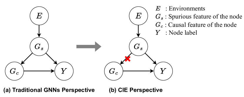
Figure 1. Causal graph on Node Classification. (a) Node classification Process from the perspective of traditional GNNs. (b) Node Classification Process Revised by CIE.

We revisit the node classification process of traditional graph neural networks from the perspective of causal learning(Pearl et al., 2000; Spirtes, 2010), and assume that the nodes in the graph are generated through a mapping $f_{gen}:\mathcal{Z}\rightarrow\mathcal{G}$, where $\mathcal{Z}\subseteq\mathbb{R}^{n}$ is the latent space and $\mathcal{G}$ is the graph space. Following the previous work(Von Kügelgen et al., 2021; Chen et al., 2022c), we divide the latent variable $\mathcal{Z}$ into spurious features $G_{s}$ and causal features $G_{c}$ according to whether it is directly affected by the environment $E$.

In theory, $G_{s}$ and $G_{c}$ are two independent subspaces of $\mathcal{Z}$ (Von Kügelgen et al., 2021; Chen et al., 2022c). However, the traditional graph neural networks focus on establishing the correlation between node features and labels under the independent and identically distributed assumption, while ignoring the fact that spurious features $G_{s}$ are easily affected by the environment $E$. Therefore, the node representations learned by the traditional graph neural networks are the fusion of $G_{s}$ and $G_{c}$. $G_{s}$ confuses the causation between causal features $G_{c}$ and labels $Y$ in the prediction stage, $Y:=f_{gnns}(G_{s},G_{c})$, as illustrated in Fig.1(a). Moreover, some recent work(Torralba and Efros, 2011; Geirhos et al., 2020; Lin et al., 2021) has found that neural networks, including graph neural networks, are more susceptible to establishing spurious correlations(Chen et al., 2020; Zhou et al., 2021; Khani and Liang, 2021) between spurious features and labels in data, which are not stable in nature.

Therefore, in this paper, we aim to address the limitations of traditional graph neural networks from a causal perspective. Specifically, we treat $G_{s}$ as a confounder on the backdoor path(Pearl, 2009; Spirtes, 2010) ($G_{c}\leftarrow G_{s}\rightarrow Y$) between $G_{c}$ and $Y$. Theoretically, we can block the above backdoor path through the backdoor adjustment(Pearl, 2009; Spirtes, 2010), since $G_{s}$ satisfies the backdoor criterion(Bareinboim and Pearl, 2016), as illustrated in Fig.1(b). Formally, we can introduce the following formula through the backdoor adjustment:

(2) $$P(Y|\operatorname{do}(G_{c})) =\sum_{s\in G_{s}}P(Y|\operatorname{do}(G_{c}),s)P(s|\operatorname{do}(G_{c}))$$

$$=\sum_{s\in G_{s}}P(Y|G_{c},s)P(s|\operatorname{do}(G_{c}))$$

$$=\sum_{s\in G_{s}}P(Y|G_{c},s)P(s),$$

where $P(Y|G_{c},s)$ represents the conditional probability of $Y$ given the causal feature $G_{c}$ and the confounder $s$, and $P(s)$ is the prior probability of the confounder.

However, the aforementioned formula presents two challenges: (1) Due to the characteristics of graph data, $G_{s}$ is typically not observable, making it difficult to directly obtain $G_{s}$ and $G_{c}$ at the data level. (2) Given that $G_{s}$ is a continuous subspace of $\mathcal{Z}$, the process of discretely integrating it is extremely challenging, as shown in Equation 2. In the rest of this paper, we dedicate to elaborating on the methodology to overcome these challenges and efficiently approximate Equation 2, demonstrating the efficiency and effectiveness.

4. METHODOLOGY

In this section, we first introduce the overall framework of the Causality and Independence Enhancement (CIE), followed by a detailed description of the proposed method.

4.1. Overall Framework

The structure of the proposed CIE framework is illustrated in Figure 2, which consists of two main steps: Estimating causal and spurious features from node representations, and Mitigating spurious correlations. Specifically, causal and spurious features are estimated from node representations by the soft mask module as well as independence constraint. In addition, spurious correlations are mitigated by blocking the backdoor path ($G_{c}\leftarrow G_{s}\rightarrow Y$) through the backdoor adjustment (approximating Equation 2).

In previous works, methods designed to address a specific type of data bias may not necessarily enhance generalization performance overall, due to the lack of global considerations. Furthermore, we found that when labeled information is insufficient, the prediction of graph structure in EERM could introduce fatal misinformation to the nodes with lower degree. Therefore, our approach debiases different types of data biases from a unified perspective, avoiding the need to design methods for each bias separately and preventing the introduction of misinformation in low-resource scenarios. Our intuition is straightforward that either feature-level bias or topology-level bias will ultimately be incorporated into the node representations in the graph neural network framework. From a causal perspective, identifying and eliminating data biases in node representations through the backdoor adjustment is a more effective and efficient approach. Moreover, the complex biased environments (especially mixed biases) makes it more difficult to disentangle the spurious features, which poses a challenge for the estimation of causal and spurious features. The introduction of independence constraint not only improves the discriminability between causal and spurious features but also enhances stability in complex biased environments. Subsequent experimental results have also confirmed our hypotheses.

Next, we provide a detailed description of the steps involved in estimating causal and spurious features and mitigating spurious correlations.

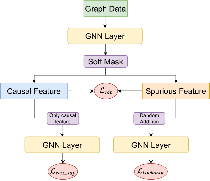
Figure 2. The overall framework of CIE.

4.2. Disentanglement from Node Representation

As previously mentioned, identifying causal and spurious features ($G_{c}$ and $G_{s}$, respectively) at the graph data level is often challenging due to the discrete nature of graph data. However, traditional graph neural networks are capable of learning representations for each node that incorporate causal and spurious features, which provides an opportunity to address the aforementioned challenge by disentangling these two types of features at the node representation level.

We introduce the soft mask module to generate two branches ($\mathbf{H_{c}}$ and $\mathbf{H_{s}}$) for estimating causal features $G_{c}$ and spurious features $G_{s}$, respectively. The soft mask module consists of $\mathbf{M_{c}}\in\mathbb{R}^{N\times 1}$, $\mathbf{M_{s}}\in\mathbb{R}^{N\times 1}$ and $\mathbf{M_{c}}+\mathbf{M_{s}}=\mathbf{1}$, where $N$ is the number of nodes and $\mathbf{1}$ is the all-one matrix.

To extract features and obtain node representations $\mathbf{H}$, we use a GNN layer to aggregate neighbor information from the graph $G=\{\mathbf{A},\mathbf{X}\}$, where $\mathbf{A}$ is the adjacency matrix and $\mathbf{X}$ is the node feature matrix. The resulting node representations $\mathbf{H}$ incorporates both spurious and causal features, as discussed in Section 3.2.

(3) $$\mathbf{H}=\operatorname{GNN}(\mathbf{A},\mathbf{X}).$$

The weight of the two branches is estimated by a multi-layer perceptron (MLP), which determines the value of the soft mask.

(4) $$\mathbf{M_{c}},\mathbf{M_{s}} =\sigma(\operatorname{MLP}(\mathbf{H}))$$

$$\mathbf{H_{c}}=\mathbf{H}\odot \mathbf{M_{c}},\;\mathbf{H_{s}}=\mathbf{H}\odot\mathbf{M_{s}},$$

where $\sigma$ is the softmax function. $\mathbf{H_{c}}$ and $\mathbf{H_{s}}$ are derived from node representations $\mathbf{H}$ containing $G_{c}$ and $G_{s}$, but they still need to satisfy the following constraints to serve as approximate estimates of $G_{c}$ and $G_{s}$:

1. Independence. $\mathbf{H_{c}}$ and $\mathbf{H_{s}}$ should be as independent as possible, as mentioned in Section 3.2 for $G_{c}$ and $G_{s}$.

2. Backdoor adjustment. The backdoor path is broken off by Equation 2 to mitigate spurious correlations, as shown in Fig.1(b).

4.3. Independence

According to the causal perspective discussed in Section 3.2, $G_{c}$ and $G_{s}$ are two subspaces of the latent space $\mathcal{Z}$ that are independent of each other. As approximate estimates of $G_{c}$ and $G_{s}$, $\mathbf{H_{c}}$ and $\mathbf{H_{s}}$ should also be as independent of each other as possible. Intuitively, independence provides greater stability and discriminability in the presence of different types of biases, as confirmed by subsequent experimental results.

We define $\mathcal{X}$ and $\mathcal{Y}$ as two spaces of $G_{c}$ and $G_{s}$, respectively, and each sampling gets a pair of causal and spurious features of a node $i$, $\{(h_{ci},h_{si})\in\mathcal{X}\times\mathcal{Y}\}$. Next, we define mapping functions $\phi(h_{ci})\in\mathcal{F}$ and $\psi(h_{si})\in\varOmega$ that map each $h_{ci}\in\mathcal{X}$ and $h_{si}\in\mathcal{Y}$ to the kernel space $\mathcal{F}$ and $\varOmega$ with respect to the kernel functions $k_{\phi}(h_{ci},h_{ci})=<\phi(h_{ci}),\phi(h_{ci})>$ and $k_{\psi}(h_{si},h_{si})=<\psi(h_{si}),\psi(h_{si})>$, respectively. $\mathcal{F}$ and $\varOmega$ are Reproducing Kernel Hilbert Space (RKHS)(Paulsen and Raghupathi, 2016) on $\mathcal{X}$ and $\mathcal{Y}$, respectively. According to (Baker, 1973; Fukumizu et al., 2004), we can define a cross-covariance operator between the above feature maps:

(5) $$\mathcal{C}_{h_{ci}h_{si}}=\mathbf{E}_{h_{ci},h_{si}}[(\phi(h_{ci})-\mu_{h_{ci}})\otimes(\psi(h_{si})-\mu_{h_{si}})],$$

where $\otimes$ is the tensor product, and $\|\mu_{h_{ci}}\|_{\mathcal{F}}^{2}$ can be calculated by applying the expectation twice via E.q.6, and $\|\mu_{h_{si}}\|_{\varOmega}^{2}$ similarly.

(6) $$\|\mu_{h_{ci}}\|_{\mathcal{F}}^{2}=\mathbf{E}_{h_{ci},h_{ci}}[k_{\phi}(h_{ci},h_{ci})].$$

Then, the square of the Hilbert-Schmidt norm of the correlated cross-covariance operator (HSIC), $\mathcal{C}_{\mathbf{H_{c}}\mathbf{H_{s}}}$ is expressed as

(7) $$\operatorname{HSIC}(\mathcal{F},\varOmega,P_{\mathbf{H_{c}},\mathbf{H_{s}}})=\|\mathcal{C}_{\mathbf{H_{c}}\mathbf{H_{s}}}\|_{\operatorname{HS}}^{2},$$

where $P_{\mathbf{H_{c}},\mathbf{H_{s}}}$ is a joint measure over $\mathcal{F}\times\varOmega$ and $\|X\|_{\operatorname{HS}}=\sqrt{\sum_{i,j}x_{i,j}^{2}}.$ Therefore, the empirical estimate of the HSIC (Gretton et al., 2005; Song et al., 2007) is given as follows

(8) $$\operatorname{HSIC}(\mathcal{F},\varOmega,Z)=(m-1)^{2}\operatorname{tr}(\mathbf{K}\mathbf{R}\mathbf{L}\mathbf{R}),$$

where $Z=\{(h_{c1},h_{s1}),...,(h_{cm},h_{sm})\}\subseteq\mathcal{F}\times\varOmega$, $\mathbf{K},\mathbf{L},\mathbf{R}\in\mathbb{R}^{m\times m}$, $\mathbf{K}_{ij}=k_{\phi}(h_{ci},h_{cj})$, $\mathbf{L}_{ij}=k_{\psi}(h_{si},h_{sj})$, and $R$ is the centering matrix $\mathbf{R}_{m}=\mathbf{I}_{m}-\frac{1}{m}\mathrm{11^{T}}$. The independence between causal and spurious features can be described by HSIC using kernel functions, with the computational complexity of $\mathcal{O}(m^{2})$, where m is the number of samples. In contrast, other kernel methods require at least $\mathcal{O}(m^{3})$(Bach and Jordan, 2002). But HSIC is not invariant to isotropic scaling, we adopt the normalized HSIC (CKA) (Kornblith et al., 2019), which is defined as follows:

(9) $$\mathcal{L}_{idp}=\operatorname{CKA}(\mathbf{H_{c}},\mathbf{H_{s}})=\frac{\operatorname{HSIC}(\mathbf{H_{c}},\mathbf{H_{s}})}{\sqrt{\operatorname{HSIC}(\mathbf{H_{c}},\mathbf{H_{c}})\operatorname{HSIC}(\mathbf{H_{s}},\mathbf{H_{s}})}}.$$

CKA describes the correlation between the causal and spurious feature subspaces. When $k_{\phi}$ and $k_{\psi}$ are universal kernels, $\operatorname{CKA}=0$ implies independence. We aim to minimize the dependency between $\mathbf{H_{c}}$ and $\mathbf{H_{s}}$ by introducing the loss as depicted in Equation 9. In the experimental section, we focus on employing radial basis functions(Buhmann, 2003) and investigate the impact of different kernel functions.

4.4. Backdoor Adjustment

Traditional graph neural networks often suffer from unstable spurious correlations between $G_{c}$ and $Y$, caused by the presence of the backdoor path ($G_{c}\leftarrow G_{s}\rightarrow Y$), as illustrated in Fig.1. It is evident that when the data does not follow the I.I.D. assumption, the spurious correlation between $G_{c}$ and $Y$ can lead to decreased performance in graph neural networks.

Our objective is to enhance the generalization performance of GNNs in the presence of different types of biases by applying the backdoor adjustment to eliminate spurious correlations. However, there exists a challenge when attempting to discretize $G_{s}$(or $H_{s}$) as described in Section 3.2. Inspired by (Pearl, 2014; Sui et al., 2022), we intervene on the backdoor path at the node representation level and introduce random addition to approximate Equation 2. Specifically, in accordance with the principles of backdoor adjustment, we hereby introduce the following loss function:

(10) $$z_{i}^{\prime}=\operatorname{GNN}(\mathbf{A}, h_{ci}+h_{sj}),\;sj\in\mathbf{H_{s}},$$

(11) $$\mathcal{L}_{backdoor}=\frac{1}{n\times|\mathbf{H_{s}}|}\sum_{i=1}^{n}\sum_{sj\in\mathbf{H_{s}}}\ell(y_{i},\sigma(z_{i}^{\prime})),$$

where $h_{ci}$ is the causal feature of node $i$ from $\mathbf{H_{s}}$, $h_{sj}$ is the spurious feature of node $j$ randomly sampled from $\mathbf{H_{s}}$, $z_{i}^{\prime}$ is the node representations after intervention, $\sigma$ is the Softmax function, $n$ is the number of training examples, and $\ell$ is the cross-entropy loss. Specifically, we assume that $P(s)$ follows a uniform distribution, and estimate $P(Y|G_{c},s)$ by $\frac{1}{n}\sum_{i=1}^{n}\ell(y_{i},\sigma(z_{i}^{\prime}))$ through randomly sampling from $\mathbf{H_{s}}$ ($\mathbf{H_{s}}$ is the approximate estimate of $G_{s}$).

Thus far, we have successfully disentangled $G_{c}$ and $G_{s}$ at the node representation level and eliminated the influence of the backdoor path between $G_{c}$ and $Y$, resulting in causal features for each node. We use the message passing mechanism to aggregate and propagate the causal features of neighboring nodes, resulting in node representations for the final classification objective.

(12) $$z_{ci}=\operatorname{GNN}(\mathbf{A},\mathbf{H_{c}}),$$

(13) $$\mathcal{L}_{cau\_sup}=\frac{1}{n}\sum_{i=0}^{n}\ell(y_{i},\sigma(z_{ci})),$$

where $z_{ci}$ is the representation for the i-th node, $n$ is the number of training examples.

In summary, the overview of CIE is shown in Figure 2, and the objective function of the CIE consists of the weighted sum of the above-mentioned losses:

(14) $$\mathcal{L}=\mathcal{L}_{cau\_sup}+\lambda_{1}\mathcal{L}_{idp}+\lambda_{2}\mathcal{L}_{backdoor}$$

where $\lambda_{1}$ and $\lambda_{2}$ are the hyperparameter weights that control each component.

Table 1. Dataset statistics

Dataset	Type	Nodes	Edges	Features	Classes
Cora	Citation Network	2,708	10556	1433	7
Citeseer	Citation Network	3327	9104	3703	6
Pubmed	Citation Network	19717	88648	500	3
NELL	Knowledge Graph	65755	251550	61278	186
Reddit	Social Network	232965	114615892	602	41

5. Experiments

In this section, we provide a detailed description of the experimental settings and evaluate the efficiency and effectiveness of our proposed method. The experiments include node classification with different types of data biases, ablation studies, parameter sensitivity analyses, and time complexity comparisons, all aimed at answering the following research questions (RQs):

• RQ1: How does CIE compare to state-of-the-art debiased node classification methods in different types of data biases? Additionally, how much improvement can it bring to the backbone models?

• RQ2: What is the impact of applying the independence constraint and backdoor adjustment on the proposed model? Can either loss function be effective when used alone?

• RQ3: How do different hyperparameters (e.g., the choice of $\lambda_{1}$ and $\lambda_{2}$) affect the performance of CIE? Additionally, how does the time efficiency of the proposed method compare to state-of-the-art methods?

5.1. Experimental Settings

To satisfy the definition of OOD, we follow the inductive setting in (Wu et al., 2019; Fan et al., 2022), masking out test nodes as $G_{train}$ during the training and validation stages, and subsequently predicting the labels of test nodes with the complete graph $G_{test}$. In this way, the test distribution is guaranteed to be agnostic during the training phase. Moreover, all of the following biases are introduced in the training graph $G_{train}$ to ensure that $P_{train}(X,Y)\neq P_{test}(X,Y)$.

5.1.1. Different biases in node classification

Currently, most existing works focus on developing algorithms for one specific type of data bias. However, this approach does not necessarily improve generalization overall, since predicting the type of data biases can be difficult in reality. Therefore, in this paper, we consider several common biases that have been explored in prior research, including label selection bias(Zadrozny, 2004; Fan et al., 2022) that can cause distribution shift at the feature level, structural bias(He et al., 2021) that can cause distribution shift at the topology level, and their mixed biases. Additionally, we introduce the small sample selection bias(Fan et al., 2022) to evaluate the performance of CIE in low-resource scenarios, which can cause distribution shift at the feature level.

5.1.2. Datasets and Bias Setting

To evaluate the performance of our proposed method under specific bias, we introduce label selection bias and structural bias on the Cora, Citeseer, and Pubmed datasets(Sen et al., 2008). Following (Fan et al., 2022), we regulate the level of data bias by adjusting the hyperparameter $\epsilon\in\{0.4,0.6,0.8\}$. Specifically, in the case of label selection bias, a higher value of $\epsilon$ indicates a greater tendency to select nodes with inconsistent labels with their neighboring nodes as the training set. In the case of structural bias, the value of $\epsilon$ represents the percentage of edges to be randomly removed from $G_{train}$. For example, $\epsilon=0.4$ indicates randomly deleting $40\%$ of the edges. We select 20 nodes from each class as the training nodes and use the training set partitioned in the original paper(Kipf and Welling, 2016; Veličković et al., 2017) as the unbiased setting.

To evaluate performance under mixed biases, we primarily introduce different degrees of label selection bias and structural bias simultaneously on three citation network datasets. We utilize the hyperparameter $\epsilon$ mentioned above to regulate the combination of these two biases at varying levels.

To evaluate performance in low-resource scenarios, we introduce small sample selection bias on NELL(Glorot and Bengio, 2010) and Reddit datasets(Hamilton et al., 2017). Specifically, we randomly select 1/3/5/10 nodes from each class as the training set. The validation set and test set remain the same as in the original paper(Veličković et al., 2017; Hamilton et al., 2017). Table 1 displays five publicly available datasets, along with their corresponding bias configurations.

5.1.3. Baselines

In order to verify the effectiveness of the proposed method CIE, we conducted a comprehensive comparison with the following eight state-of-the-art methods, which can be classified into three categories: (1) Backbone models, such as GCN (Kipf and Welling, 2016), GraphSAGE (Hamilton et al., 2017), and GAT (Veličković et al., 2017). Our method can be directly applied to backbone models to improve their generalization. The improvement in the performance of backbone models can directly validate the effectiveness of the proposed method. (2) Node classification models. In addition to backbone networks, there have been outstanding works such as SGC(Wu et al., 2019) and APPNP(Klicpera et al., 2018) aimed at improving the performance of node classification. (3) Debiased node classification models. Methods tailored to address a specific type of data bias, including CATs(He et al., 2021), DGNN(Fan et al., 2022), and EERM(Wu et al., 2022), represent strong baselines in this field. For DGNN, we compared two variants: DGCN and DGAT. As for EERM, we utilized the best performing version based on GAT.

5.1.4. Implementation Details

We implemented our proposed model based on PyTorch and PyTorch Geometric. For all baselines, all hyperparameter settings are based on the reports in the original papers to achieve optimal results. For our proposed model, in order to make a fair comparison, we adopt a two-layer architecture for GNNs, where we sample 25 and 10 neighbors separately if it involves the SAGE layer. We use Adam as the optimizer, with a learning rate of 0.01. The hyperparameters $\lambda_{1}$ and $\lambda_{2}$ are tuned in the range of $\{0.1,0.2,0.3,...,0.9,1.0\}$, while dropout is set to 0.5 or 0.6. We set other parameters, such as the number of attention heads in the GAT layer and the embedding size, based on the specifications in the original paper for the backbone model. We conducted each experiment 10 times with different random seeds and reported the average accuracy. All experiments were conducted on Ubuntu 20.04 with NVIDIA RTX A6000 GPUs.

5.2. Performance on Complex Biases (RQ1)

To validate the effectiveness of our approach, we extensively compared CIE with state-of-the-art baselines on complex data biases, as detailed in Section 5.1. Furthermore, we evaluated whether CIE is effective in low-resource scenarios by introducing the small sample selection bias. Finally, we provided a comprehensive analysis and discussion of each experiment in Section 5.2.4.

5.2.1. A Specific Type of Data Bias.

To compare the performance of our proposed method with state-of-the-art methods under a specific type of bias, we separately introduce label selection bias and structural bias on three citation networks, and control the degree of each bias through $\epsilon$. As shown in Table 2 and 3, we have the following findings:

• Models that are tailored to address a specific type of data bias may exhibit suboptimal performance when deployed in other biases, occasionally even underperforming compared to GAT. Our empirical findings show that merely pursuing a specific type of data bias is inadequate to improve generalization performance overall, due to the challenge in anticipating the type of data biases in advance.

• In the experiments with a specific type of data bias, our proposed CIE significantly and consistently improves the performance of all backbone models, surpassing all state-of-the-art methods for debiased node classification.

• Our proposed method outperforms because the methods designed for specific types of bias lack global considerations. CIE considers the biases inherent in feature and structural information from a unified perspective, avoiding the challenge of designing for each bias separately.

Table 2. Performance of label selection bias in three citation networks. The * indicates the best results of the baselines. Best results of all methods are indicated in bold. ‘% gain over GNN’ means the improvement percent against GNN (the same below).

Method	Cora				Citeseer				Pubmed
	unbiased	0.4	0.6	0.8	unbiased	0.4	0.6	0.8	unbiased	0.4	0.6	0.8
SGC	0.7710	0.7723	0.7417	0.7330	0.6803	0.6717	0.6137	0.6480	0.7750	0.7477	0.7490	0.7517
APPNP	0.8078	0.7808	0.7566	0.7336	0.6656	0.6474	0.6084	0.5842	0.7703	0.7650	0.7581	0.7574
CATs	0.8093	0.7883	0.7560	0.7070	0.7017	0.7083	0.6593	0.6510	0.7770	$\mathbf{0.7777^{*}}$	0.7613	0.7620
DGCN	0.7947	0.7869	0.7653	0.7189	0.6734	0.6704	0.6349	0.6169	0.7849	0.7619	0.7680	0.7694
DGAT	$0.8141^{*}$	$0.7950^{*}$	$0.7775^{*}$	$0.7579^{*}$	$0.7070^{*}$	$0.7132^{*}$	$0.6861^{*}$	$0.6705^{*}$	0.7812	0.7671	$0.7717^{*}$	0.7713
EERM	0.7974	0.7914	0.7698	0.7496	0.6986	0.7034	0.6764	0.6606	0.7754	0.7646	0.7675	0.7526
SAGE	0.7822	0.7803	0.7377	0.7118	0.6824	0.6649	0.6723	0.6313	0.7721	0.7461	0.7424	0.7479
SAGE_CIE	0.7944	0.7950	0.7537	0.7239	0.7038	0.6947	0.6975	0.6761	0.7741	0.7506	0.7534	0.7608
% gain over SAGE	1.56%	1.89%	2.16%	1.69%	3.14%	4.49%	3.76%	7.09%	0.25%	0.61%	1.49%	1.73%
GCN	0.7834	0.7777	0.7552	0.7101	0.6681	0.6634	0.6231	0.5877	0.7833	0.7536	0.7602	$0.7714^{*}$
GCN_CIE	0.8063	0.7999	0.7720	0.7285	0.6859	0.6822	0.6572	0.6231	0.7908	0.7689	0.7769	0.7776
% gain over GCN	2.92%	2.85%	2.22%	2.59%	2.66%	2.83%	5.48%	6.03%	0.97%	2.03%	2.20%	0.80%
GAT	0.8028	0.7850	0.7727	0.7381	0.7013	0.7047	0.6776	0.6544	$0.7833^{*}$	0.7596	0.7668	0.7681
GAT_CIE	0.8228	0.8047	0.7803	0.7627	0.7137	0.7236	0.7101	0.6799	0.7889	0.7721	0.7753	0.7763
% gain over GAT	2.49%	2.50%	0.99%	3.33%	1.77%	2.69%	4.80%	3.90%	0.71%	1.65%	1.12%	1.07%

Table 3. Performance of structural bias in three citation networks.

Method	Cora				Citeseer				Pubmed
	unbiased	0.4	0.6	0.8	unbiased	0.4	0.6	0.8	unbiased	0.4	0.6	0.8
SGC	0.7710	0.7640	0.7690	0.7707	0.6803	0.6917	0.6783	0.6894	0.7750	0.7653	$0.7703^{*}$	0.7623
APPNP	0.8078	0.7653	0.7462	0.7416	0.6656	0.6502	0.6258	0.6166	0.7703	0.7510	0.7661	0.7450
CATs	0.8093	$0.8043^{*}$	$0.7930^{*}$	$0.7760^{*}$	0.7017	$0.6983^{*}$	$0.6867^{*}$	$0.6993^{*}$	0.7770	$0.7707^{*}$	0.7677	$\mathbf{0.7660^{*}}$
DGCN	0.7947	0.7697	0.7524	0.7422	0.6734	0.6369	0.6407	0.6397	0.7849	0.7556	0.7594	0.7435
DGAT	$0.8141^{*}$	0.8014	0.7817	0.7701	$0.7070^{*}$	0.6933	0.6837	0.6860	0.7812	0.7665	0.7647	0.7563
EERM	0.7974	0.7858	0.7694	0.7638	0.6986	0.6806	0.6716	0.6808	0.7754	0.7682	0.7672	0.7468
SAGE	0.7822	0.7474	0.6969	0.6007	0.6824	0.6557	0.6463	0.6439	0.7721	0.7488	0.7484	0.7293
SAGE_CIE	0.7944	0.7664	0.7141	0.6502	0.7038	0.7008	0.6689	0.6803	0.7741	0.7603	0.7608	0.7365
% gain over SAGE	1.56%	2.54%	2.46%	8.25%	3.14%	6.87%	3.50%	5.65%	0.25%	1.54%	1.66%	0.98%
GCN	0.7834	0.7442	0.7246	0.6993	0.6681	0.6252	0.6278	0.6113	0.7833	0.7607	0.7587	0.7446
GCN_CIE	0.8063	0.7784	0.7563	0.7444	0.6859	0.6565	0.6664	0.6610	0.7908	0.7619	0.7672	0.7556
% gain over GCN	2.92%	4.60%	4.38%	6.44%	2.66%	5.01%	6.14%	8.13%	0.97%	0.17%	1.12%	1.48%
GAT	0.8028	0.7833	0.7618	0.7429	0.7013	0.6885	0.6611	0.6737	$0.7833^{*}$	0.7679	0.7684	0.7517
GAT_CIE	0.8228	0.8109	0.7937	0.7834	0.7137	0.7024	0.6982	0.7062	0.7889	0.7783	0.7732	0.7561
% gain over GAT	2.49%	3.52%	4.19%	5.46%	1.77%	2.03%	5.61%	4.82%	0.71%	1.35%	0.62%	0.59%

5.2.2. Mixed Biases

In real-world applications, models are often affected by multiple types of biases simultaneously, such as both label selection bias and structural bias, which is a more challenging and important issue. To evaluate the performance of our proposed method under mixed biases, we introduce label selection bias and structural bias simultaneously on three citation networks as an illustration, and compare it with state-of-the-art methods. As shown in Table 4 (due to space limitations, the performance on the other two datasets is similar and can be found here.) , we have the following findings:

• Our proposed method significantly improves the generalization performance of the backbone model, even under mixed biases. By adopting a unified perspective on the distribution shift of feature and topology levels, CIE enables the model to effectively handle multiple types of biases simultaneously.

• Mixed biases have a more substantial influence on models than any specific type of bias. Nevertheless, in the experiments with mixed biases, the proposed method CIE consistently outperforms state-of-the-art debiased node classification methods by a considerable margin.

Table 4. Performance of mixed biases (Label selection bias and Structural bias) on Cora.

Label selection bias	0.4			0.6			0.8
Structural bias	0.4	0.6	0.8	0.4	0.6	0.8	0.4	0.6	0.8
SGC	0.7210	0.7100	0.6750	0.7240	0.6825	0.5925	0.7220	0.6800	0.6550
APPNP	0.7430	0.6880	0.6520	0.7350	0.7400	0.6780	0.7190	0.6930	0.6780
CAT	0.7780	0.7505	0.7425	0.7255	0.7400	0.6935	0.7015	0.6885	$0.6970^{*}$
DGCN	0.7805	0.7165	0.7635	0.7195	0.7080	0.7125	0.6870	0.6970	0.6580
DGAT	$0.7900^{*}$	$0.7560^{*}$	$0.7670^{*}$	$0.7420^{*}$	0.7115	0.6975	$0.7220^{*}$	0.7220	0.6710
EERM	0.7714	0.7363	0.7311	0.7368	0.7192	0.7012	0.7163	0.6906	0.6728
SAGE	0.7650	0.7125	0.6435	0.6960	0.6655	0.5450	0.6370	0.6115	0.4660
SAGE_CIL	0.7795	0.7435	0.7070	0.7150	0.7190	0.6680	0.6935	0.6695	0.5650
% gain over SAGE	1.90%	4.35%	9.87%	2.73%	8.04%	22.57%	8.87%	9.48%	21.24%
GCN	0.7693	0.7417	0.7253	0.7400	0.7113	0.6920	0.6893	0.7107	0.6303
GCN_CIL	0.7965	0.7595	0.7530	0.7590	0.7555	0.7100	0.7165	0.7255	0.6515
% gain over GCN	3.53%	2.40%	3.81%	2.57%	6.21%	2.60%	3.94%	2.09%	3.36%
GAT	0.7835	0.7460	0.7585	0.7405	$0.7565^{*}$	$0.7360^{*}$	0.7200	$0.7330^{*}$	0.6965
GAT_CIL	0.7965	0.7570	0.7900	0.7610	0.7575	0.7420	0.7565	0.7730	0.7210
% gain over GAT	1.66%	1.47%	4.15%	2.77%	0.13%	0.82%	5.07%	5.46%	3.52%

5.2.3. Evaluation in low-resource Scenarios.

To evaluate the performance of CIE in low-resource scenarios, we introduce the small sample selection bias on NELL and Reddit datasets. Due to the difficulty of most baselines in running on these datasets and not supporting neighbor sampling, we compare our method with MLP and backbone models using neighbor sampling. As shown in Table 5, we found that even in low-resource scenarios, our method can effectively improve the performance of backbone models. Furthermore, as the number of annotated nodes decreases, the improvement relative to the backbone model becomes more significant, further demonstrating the effectiveness of our method.

Table 5. Performance of low-resource scenarios. ${\dagger}$ means GCN/GCN_CIE for NELL and SAGE/SAGE_CIE for Reddit.

Method	NELL-1	NELL-3	NELL-5	NELL-10	Reddit-1	Reddit-3	Reddit-5	Reddit-10
MLP	0.1816	0.3261	0.4685	0.5552	0.1359	0.1948	0.2433	0.2991
$\rm SAGE^{\dagger}$	0.6233	0.6718	0.7812	0.7925	0.3558	0.5060	0.6722	0.7861
$\rm SAGE\_CIE^{\dagger}$	0.6409	0.6945	0.7988	0.8019	0.4207	0.5480	0.7125	0.8145
% gain over GCN	2.82%	3.38%	2.25%	1.19%	18.23%	8.30%	6.00%	3.61%
GAT	$0.6718^{*}$	$0.7114^{*}$	$0.7822^{*}$	$0.8101^{*}$	$0.7075^{*}$	$0.8663^{*}$	$0.8902^{*}$	$0.9052^{*}$
GAT_CIE	0.7079	0.7988	0.7977	0.8111	0.7663	0.8774	0.9122	0.9195
% gain over GAT	5.37%	12.29%	1.98%	0.12%	8.31%	1.29%	2.47%	1.58%

5.2.4. Discussion and Analysis

Traditional node classification models neither distinguish between spurious features and causal features nor consider the susceptibility of spurious features to biases, which leads to performance degradation. However, due to the selective aggregation of neighbor information (attention mechanisms), GAT generally outperforms other models such as GCN in most cases. In debiased node classification methods, CATs are only designed to address structural bias, EERM requires sufficient labeled information to estimate and enrich the multiple environments, while DGNN is only designed to the feature-level distribution shift. These methods are insufficient in addressing complex data biases, especially mixed biases. DGNN estimates the weights of labeled nodes from a causal perspective, which in some cases can alleviate the interference of structural bias. Therefore, DGNN achieves some favorable results compared to other baselines, but is still inferior to our proposed method. Due to the requirement of a large amount of annotated information to generate multiple environments, EERM’s performance in various semi-supervised and low-resource scenarios in this paper is not satisfactory and even inferior to models designed for specific biases. For structural bias, we did not predict potential structures as EERM did because we found that this would introduce fatal erroneous information to the nodes with lower degrees. Our proposed method takes a unified perspective on different types of biases: whether it will result in distribution shift at the feature level or topology level, both will affect the learning of node representations after information aggregation via GNNs. Therefore, we constrain the model to learn causal features and mitigate spurious correlations at the node representation level. This approach not only avoids the challenge of designing for each type of bias as in previous work, but also enables the model to handle multiple types of biases simultaneously under mixed biases. Experimental results confirm the effectiveness of our method.

In summary, the above experimental results effectively validate the effectiveness of the proposed method under different types of biases and mixed biases. The proposed method CIE not only significantly improves the generalization performance of the backbone model but also surpasses state-of-the-art debiased node classification methods.

5.3. Ablation Study and Sensitivity Analysis (RQ2 & RQ3)

5.3.1. Ablation Study

In this section, we investigate the impact of the independence constraint and backdoor adjustment on overall performance through ablation experiments. As shown in Table 3, in most cases, using independence constraint or backdoor adjustment alone can improve generalization performance, but not stably. Intuitively, the independence constraint emphasize the independence of causal features and spurious features in subspaces, aiming to enhance the separation effect. The backdoor adjustment, on the other hand, aim to mitigate the impact of spurious correlation on the backdoor path. The joint effect of independence constraint and backdoor adjustment can significantly improve the generalization performance of the backbone model while maintaining stability.

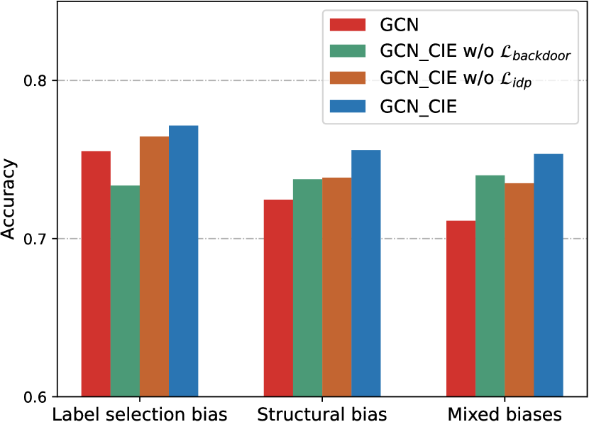
Figure 3. Ablation Study. ”w/o” means ”without”.

5.3.2. Parameter Sensitivity.

We investigate the sensitivity of the parameters under different types of biases and report the results in Fig. 5. We select GAT as the backbone model, fix one parameter to 0.5, and the other parameter changes in [0,1] with a step size of 0.1. The results show that the proposed method is relatively stable in most cases for the variation of $\lambda$, but fluctuates more in the small sample selection bias. An intuitive explanation is that the limited amount of information provided when there are only a few samples per class makes it demand higher requirements for hyperparameters. It is also worth noting that even in cases of fluctuations, there is a significant improvement in the performance of the backbone model, as shown in Table 5 and Fig.5.

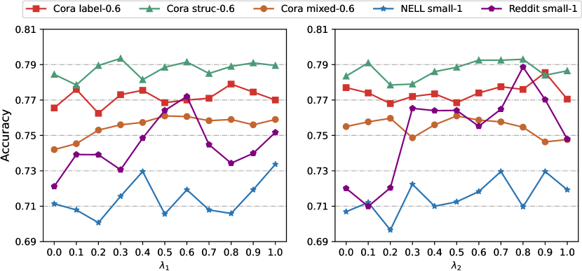
Figure 4. Parameter sensitivity of $\lambda_{1}$ and $\lambda_{2}$. ”Cora label-0.6” denotes Label selection bias on Cora with $\epsilon$=0.6, ”NELL small-1” denotes small sample selection bias on Nell with 1 samples per class.

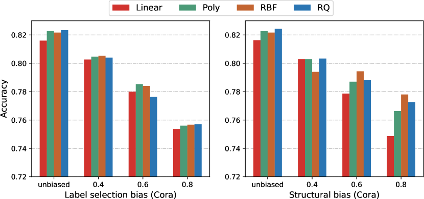
Figure 5. Sensitivity of the kernel function.

5.3.3. Sensitivity of the kernel function.

To investigate the sensitivity of the proposed method to the kernel function, we fixed other parameters($\lambda_{1}=0.5,\lambda_{2}=0.5$), changed the linear kernel, polynomial kernel function (p=2, Poly), Radial Basis Function(RBF) and rational quadratic kernel (RQ), and the experimental results are shown in Fig. 5. In most cases, RBF and RQ are capable of achieving superior results. It is evident that more complex kernel functions usually bring more significant improvements, especially when the model faces more complex biases.

5.3.4. The computational complexity.

We theoretically analyze the computational complexity of CIE. The computational complexity of CIE is $\mathcal{O}(m^{2})$, mainly from $\mathcal{L}_{idp}$, where $m$ is the number of training instances. The computational complexity of GNNs is mostly linear in the number of edges $|E|$ of the graph, e.g. the complexity of a single-layer GCN is $\mathcal{O}(|E|CHF)$ (Kipf and Welling, 2016). Therefore, the overall complexity of GCN_CIE is $\mathcal{O}(|E|CHF+m^{2})$. We report the results of the average training time per epoch on different datasets, measured in seconds and shown in Table 6. Due to the typically small size of $m$ in semi-supervised node classification, the time complexity of CIE is on the same order of magnitude as the backbone model. Moreover, CIE outperforms state-of-the-art debiased node classification models in terms of performance, while also exhibiting lower time complexity.

Table 6. The training time per epoch (in seconds).

	Cora	Citeseer	Pubmed
GCN	$7.14\times 10^{-3}$	$1.35\times 10^{-2}$	$1.26\times 10^{-2}$
GATs	$4.87\times 10^{-2}$	$5.08\times 10^{-2}$	$5.11\times 10^{-2}$
DGCN	$4.11\times 10^{-2}$	$5.35\times 10^{-2}$	$6.52\times 10^{-2}$
EERM	$5.23\times 10^{-2}$	$9.70\times 10^{-2}$	$1.84$
GCN_CIE	$1.60\times 10^{-2}$	$2.31\times 10^{-2}$	$2.74\times 10^{-2}$

6. Conclusion

In this paper, we propose a novel Causality and Independence Enhancement (CIE) framework, which takes a unified approach to handling multiple types of data biases simultaneously, eliminating the need for separately designed methods for each bias as in previous works. Specifically, it estimates causal and spurious features from node representations and mitigates spurious correlations through the backdoor adjustment. Furthermore, we introduce the independence constraint to enhance the discriminability and stability of causal and spurious features in complex biased environments. Extensive experiments demonstrate the effectiveness and flexibility of CIE. In future work, we aim to apply CIE to other tasks in different fields, such as out-of-distribution generalization in computer vision.

- (1)
- Ahmed et al. (2020) Faruk Ahmed, Yoshua Bengio, Harm van Seijen, and Aaron Courville. 2020. Systematic generalisation with group invariant predictions. In ICLR.
- Arjovsky et al. (2019) Martin Arjovsky, Léon Bottou, Ishaan Gulrajani, and David Lopez-Paz. 2019. Invariant risk minimization. arXiv preprint arXiv:1907.02893 (2019).
- Bach and Jordan (2002) Francis R Bach and Michael I Jordan. 2002. Kernel independent component analysis. Journal of machine learning research 3, Jul (2002), 1–48.
- Baker (1973) Charles R Baker. 1973. Joint measures and cross-covariance operators. Trans. Amer. Math. Soc. 186 (1973), 273–289.
- Bareinboim and Pearl (2016) Elias Bareinboim and Judea Pearl. 2016. Causal inference and the data-fusion problem. Proceedings of the National Academy of Sciences 113, 27 (2016), 7345–7352.
- Buhmann (2003) Martin D Buhmann. 2003. Radial basis functions: theory and implementations. Vol. 12. Cambridge university press.
- Chen et al. (2022a) Guoxin Chen, Yongqing Wang, Jiangli Shao, Boshen Shi, Huawei Shen, and Xueqi Cheng. 2022a. InDNI: An Infection Time Independent Method for Diffusion Network Inference. In China Conference on Information Retrieval. Springer, 63–75.
- Chen et al. (2020) Yining Chen, Colin Wei, Ananya Kumar, and Tengyu Ma. 2020. Self-training avoids using spurious features under domain shift. NeurIPS 33 (2020), 21061–21071.
- Chen et al. (2022c) Yongqiang Chen, Yonggang Zhang, Yatao Bian, Han Yang, MA Kaili, Binghui Xie, Tongliang Liu, Bo Han, and James Cheng. 2022c. Learning causally invariant representations for out-of-distribution generalization on graphs. NeurIPS 35 (2022), 22131–22148.
- Chen et al. (2022b) Zhengyu Chen, Teng Xiao, and Kun Kuang. 2022b. BA-GNN: On learning bias-aware graph neural network. In 2022 IEEE 38th International Conference on Data Engineering (ICDE). IEEE, 3012–3024.
- Choi et al. (2022) Yoonhyuk Choi, Jiho Choi, Taewook Ko, Hyungho Byun, and Chong-Kwon Kim. 2022. Finding Heterophilic Neighbors via Confidence-based Subgraph Matching for Semi-supervised Node Classification. In Proceedings of the 31st ACM International Conference on Information & Knowledge Management. 283–292.
- Defferrard et al. (2016) Michaël Defferrard, Xavier Bresson, and Pierre Vandergheynst. 2016. Convolutional neural networks on graphs with fast localized spectral filtering. NeurIPS 29 (2016).
- Fan et al. (2022) Shaohua Fan, Xiao Wang, Chuan Shi, Kun Kuang, Nian Liu, and Bai Wang. 2022. Debiased graph neural networks with agnostic label selection bias. IEEE Transactions on Neural Networks and Learning Systems (2022).
- Fukumizu et al. (2004) Kenji Fukumizu, Francis R Bach, and Michael I Jordan. 2004. Dimensionality reduction for supervised learning with reproducing kernel Hilbert spaces. Journal of Machine Learning Research 5, Jan (2004), 73–99.
- Gao et al. (2023) Irena Gao, Shiori Sagawa, Pang Wei Koh, Tatsunori Hashimoto, and Percy Liang. 2023. Out-of-Domain Robustness via Targeted Augmentations. arXiv preprint arXiv:2302.11861 (2023).
- Geirhos et al. (2020) Robert Geirhos, Jörn-Henrik Jacobsen, Claudio Michaelis, Richard Zemel, Wieland Brendel, Matthias Bethge, and Felix A Wichmann. 2020. Shortcut learning in deep neural networks. Nature Machine Intelligence 2, 11 (2020), 665–673.
- Glorot and Bengio (2010) Xavier Glorot and Yoshua Bengio. 2010. Understanding the difficulty of training deep feedforward neural networks. In Proceedings of the thirteenth international conference on artificial intelligence and statistics. JMLR Workshop and Conference Proceedings, 249–256.
- Gretton et al. (2005) Arthur Gretton, Olivier Bousquet, Alex Smola, and Bernhard Schölkopf. 2005. Measuring statistical dependence with Hilbert-Schmidt norms. In International conference on algorithmic learning theory. Springer, 63–77.
- Hamilton et al. (2017) Will Hamilton, Zhitao Ying, and Jure Leskovec. 2017. Inductive representation learning on large graphs. NeurIPS 30 (2017).
- He et al. (2021) Tiantian He, Yew Soon Ong, and Lu Bai. 2021. Learning conjoint attentions for graph neural nets. NeurIPS 34 (2021), 2641–2653.
- Hendrycks and Gimpel (2016) Dan Hendrycks and Kevin Gimpel. 2016. A baseline for detecting misclassified and out-of-distribution examples in neural networks. arXiv preprint arXiv:1610.02136 (2016).
- Khani and Liang (2021) Fereshte Khani and Percy Liang. 2021. Removing spurious features can hurt accuracy and affect groups disproportionately. In Proceedings of the 2021 ACM conference on fairness, accountability, and transparency. 196–205.
- Kipf and Welling (2016) Thomas N Kipf and Max Welling. 2016. Semi-supervised classification with graph convolutional networks. arXiv preprint arXiv:1609.02907 (2016).
- Klicpera et al. (2018) Johannes Klicpera, Aleksandar Bojchevski, and Stephan Günnemann. 2018. Predict then propagate: Graph neural networks meet personalized pagerank. arXiv preprint arXiv:1810.05997 (2018).
- Kornblith et al. (2019) Simon Kornblith, Mohammad Norouzi, Honglak Lee, and Geoffrey Hinton. 2019. Similarity of neural network representations revisited. In ICML. PMLR, 3519–3529.
- Li et al. (2022a) Haoyang Li, Xin Wang, Ziwei Zhang, and Wenwu Zhu. 2022a. Out-of-distribution generalization on graphs: A survey. arXiv preprint arXiv:2202.07987 (2022).
- Li et al. (2022c) Haoyang Li, Ziwei Zhang, Xin Wang, and Wenwu Zhu. 2022c. Learning invariant graph representations for out-of-distribution generalization. In NeurIPS.
- Li et al. (2022b) Zenan Li, Qitian Wu, Fan Nie, and Junchi Yan. 2022b. GraphDE: A generative framework for debiased learning and out-of-distribution detection on graphs. NeurIPS 35 (2022), 30277–30290.
- Lin et al. (2021) Wanyu Lin, Hao Lan, and Baochun Li. 2021. Generative causal explanations for graph neural networks. In ICML. PMLR, 6666–6679.
- Liu et al. (2020) Weitang Liu, Xiaoyun Wang, John Owens, and Yixuan Li. 2020. Energy-based out-of-distribution detection. NeurIPS 33 (2020), 21464–21475.
- Paulsen and Raghupathi (2016) Vern I Paulsen and Mrinal Raghupathi. 2016. An introduction to the theory of reproducing kernel Hilbert spaces. Vol. 152. Cambridge university press.
- Pearl (2009) Judea Pearl. 2009. Causal inference in statistics: An overview. Statistics surveys 3 (2009), 96–146.
- Pearl (2014) Judea Pearl. 2014. Interpretation and identification of causal mediation. Psychological methods 19, 4 (2014), 459.
- Pearl et al. (2000) Judea Pearl et al. 2000. Models, reasoning and inference. Cambridge, UK: CambridgeUniversityPress 19, 2 (2000).
- Qu et al. (2021) Liang Qu, Huaisheng Zhu, Ruiqi Zheng, Yuhui Shi, and Hongzhi Yin. 2021. Imgagn: Imbalanced network embedding via generative adversarial graph networks. In Proceedings of the 27th ACM SIGKDD Conference on Knowledge Discovery & Data Mining. 1390–1398.
- Ren et al. (2022) Jie Ren, Jiaming Luo, Yao Zhao, Kundan Krishna, Mohammad Saleh, Balaji Lakshminarayanan, and Peter J Liu. 2022. Out-of-Distribution Detection and Selective Generation for Conditional Language Models. arXiv preprint arXiv:2209.15558 (2022).
- Rosenfeld et al. (2020) Elan Rosenfeld, Pradeep Ravikumar, and Andrej Risteski. 2020. The risks of invariant risk minimization. arXiv preprint arXiv:2010.05761 (2020).
- Sen et al. (2008) Prithviraj Sen, Galileo Namata, Mustafa Bilgic, Lise Getoor, Brian Galligher, and Tina Eliassi-Rad. 2008. Collective classification in network data. AI magazine 29, 3 (2008), 93–93.
- Shen et al. (2021) Zheyan Shen, Jiashuo Liu, Yue He, Xingxuan Zhang, Renzhe Xu, Han Yu, and Peng Cui. 2021. Towards out-of-distribution generalization: A survey. arXiv preprint arXiv:2108.13624 (2021).
- Song et al. (2007) Le Song, Alex Smola, Arthur Gretton, Karsten M Borgwardt, and Justin Bedo. 2007. Supervised feature selection via dependence estimation. In ICML. 823–830.
- Spirtes (2010) Peter Spirtes. 2010. Introduction to causal inference. Journal of Machine Learning Research 11, 5 (2010).
- Sui et al. (2022) Yongduo Sui, Xiang Wang, Jiancan Wu, Min Lin, Xiangnan He, and Tat-Seng Chua. 2022. Causal attention for interpretable and generalizable graph classification. In Proceedings of the 28th ACM SIGKDD Conference on Knowledge Discovery and Data Mining. 1696–1705.
- Tang et al. (2020) Xianfeng Tang, Huaxiu Yao, Yiwei Sun, Yiqi Wang, Jiliang Tang, Charu Aggarwal, Prasenjit Mitra, and Suhang Wang. 2020. Investigating and mitigating degree-related biases in graph convoltuional networks. In Proceedings of the 29th ACM International Conference on Information & Knowledge Management. 1435–1444.
- Torralba and Efros (2011) Antonio Torralba and Alexei A Efros. 2011. Unbiased look at dataset bias. In CVPR 2011. IEEE, 1521–1528.
- Veličković et al. (2017) Petar Veličković, Guillem Cucurull, Arantxa Casanova, Adriana Romero, Pietro Lio, and Yoshua Bengio. 2017. Graph attention networks. arXiv preprint arXiv:1710.10903 (2017).
- Von Kügelgen et al. (2021) Julius Von Kügelgen, Yash Sharma, Luigi Gresele, Wieland Brendel, Bernhard Schölkopf, Michel Besserve, and Francesco Locatello. 2021. Self-supervised learning with data augmentations provably isolates content from style. NeurIPS 34 (2021), 16451–16467.
- Wang et al. (2022) Yu Wang, Yuying Zhao, Neil Shah, and Tyler Derr. 2022. Imbalanced graph classification via graph-of-graph neural networks. In Proceedings of the 31st ACM International Conference on Information & Knowledge Management. 2067–2076.
- Wu et al. (2019) Felix Wu, Amauri Souza, Tianyi Zhang, Christopher Fifty, Tao Yu, and Kilian Weinberger. 2019. Simplifying graph convolutional networks. In ICML. PMLR, 6861–6871.
- Wu et al. (2022) Qitian Wu, Hengrui Zhang, Junchi Yan, and David Wipf. 2022. Handling distribution shifts on graphs: An invariance perspective. arXiv preprint arXiv:2202.02466 (2022).
- Wu et al. (2020) Zonghan Wu, Shirui Pan, Fengwen Chen, Guodong Long, Chengqi Zhang, and S Yu Philip. 2020. A comprehensive survey on graph neural networks. IEEE transactions on neural networks and learning systems 32, 1 (2020), 4–24.
- Yang et al. (2022) Nianzu Yang, Kaipeng Zeng, Qitian Wu, Xiaosong Jia, and Junchi Yan. 2022. Learning substructure invariance for out-of-distribution molecular representations. In NeurIPS.
- Ye et al. (2021) Haotian Ye, Chuanlong Xie, Tianle Cai, Ruichen Li, Zhenguo Li, and Liwei Wang. 2021. Towards a theoretical framework of out-of-distribution generalization. Advances in Neural Information Processing Systems 34 (2021), 23519–23531.
- Zadrozny (2004) Bianca Zadrozny. 2004. Learning and evaluating classifiers under sample selection bias. In ICML. 114.
- Zhou et al. (2021) Chunting Zhou, Xuezhe Ma, Paul Michel, and Graham Neubig. 2021. Examining and combating spurious features under distribution shift. In ICML. PMLR, 12857–12867.
- Zhuang and Al Hasan (2022) Jun Zhuang and Mohammad Al Hasan. 2022. Robust Node Classification on Graphs: Jointly from Bayesian Label Transition and Topology-based Label Propagation. In Proceedings of the 31st ACM International Conference on Information & Knowledge Management. 2795–2805.