Majorana Fermi surface state in a network of quantum spin chains

Abstract

We use junctions of critical spin-1 chains as the basic elements to construct a honeycomb network that harbors a gapless chiral spin liquid phase. The low-energy modes are described by spin-1 Majorana fermions that form a two-dimensional Fermi surface when the interactions at the junctions are tuned to the vicinity of chiral fixed points with staggered chirality. We discuss the physical properties and the stability of this chiral spin liquid phase against perturbations from the point of view of the effective field theory for the network. We find clear connections with the excitation spectrum obtained in parton constructions on the kagome lattice.

I Introduction

Mott insulators can display exotic quantum phases in which spin fractionalization gives rise to low-energy fermionic excitations [1]. In materials regarded as quantum spin liquid candidates [2, 3, 4], the observation of a constant magnetic susceptibility, linear specific heat and linear thermal conductivity at low temperatures is often interpreted as evidence for a Fermi surface of fractionalized excitations. Within effective theory descriptions [5], these gapless fermionic modes are strongly coupled to emergent gauge fields, and one may question whether these phases remain stable when interactions are treated beyond the mean-field level [6, 7, 8].

Quantum spin liquids with Fermi surfaces become more stable when the gauge structure is discrete and time reversal and inversion symmetries are broken [9]. As opposed to a U(1) spin liquid, whose gapless photon-like modes mediate long-range interactions between fermions, a $\mathbb{Z}_{2}$ spin liquid has gapped vortex-like excitations known as visons [10]. Gauge-field fluctuations can be safely neglected in the limit where visons have a large gap and a small effective bandwidth. In addition, breaking time reversal and inversion symmetries, as in chiral spin liquids (CSLs) [11], protects the Fermi surface against pairing instabilities [9, 12]. In fact, gapless CSL phases have been found in numerical studies of lattice models where time reversal symmetry is broken either spontaneously or by three-spin interactions [13, 14, 15]. In these cases, the formation of the Fermi surface is associated with a staggered scalar spin chirality on frustrated lattices. Moreover, there are examples of exactly solvable models where spins fractionalize into Majorana fermions and static $\mathbb{Z}_{2}$ gauge fields, and the Majorana fermions form a stable Fermi surface [16, 17, 18, 19, 20].

In this work we present an analytical approach that employs quantum spin chains coupled by time-reversal-symmetry-breaking interactions as building blocks of a Majorana Fermi surface state. Arrays of one-dimensional (1D) systems have been shown to realize both gapped [21, 22, 23, 24, 25, 26] and gapless [27, 28] spin liquids. Such coupled-wire constructions usually hinge on the assumption of a renormalization group (RG) flow of judiciously selected interchain interactions to strong coupling. By contrast, here we start from junctions of spin chains with boundary interactions tuned to a chiral fixed point [29, 30, 31, 32]. When the spin chains are coupled to form a network with uniform spin chirality at the junctions, this approach leads to gapped CSLs with Abelian [33] or non-Abelian [34] topological order. Our goal here is to show that the same approach applied to a network with staggered spin chirality describes a gapless CSL with a Fermi surface descended from the chiral 1D modes.

To construct a $\mathbb{Z}_{2}$ CSL with a Majorana Fermi surface, we consider a network of critical spin-1 chains described by the SU(2)₂ Wess-Zumino-Novikov-Witten (WZNW) model [35]. The latter is a conformal field theory (CFT) with central charge $c=3/2$ and admits a representation in terms of three Majorana fermions for each chain [36, 37]. The conditions for reaching the chiral fixed point of a junction of three spin-1 chains were discussed in Ref. [32]. Imposing a staggered chirality pattern on the junctions forming a honeycomb network, we show that the low-energy excitations of the system are chiral Majorana modes that run along three zigzag directions in the network. We then consider the leading perturbations allowed by symmetry when the model parameters deviate from the chiral fixed point. The theory contains a marginal operator that introduces backscattering of Majorana fermions at the junctions and can be treated exactly. This operator turns the fermionic spectrum into an authentic 2D dispersion with a line Fermi surface, closely related to that obtained in parton mean-field theories with Majorana fermions on the kagome and triangular lattices [14, 38]. We also analyze the effects of the operator associated with the spin-1/2 primary field of the SU(2)₂ WZNW model. While this perturbation is strongly relevant at the 1D fixed point, we show that deep in the 2D regime this operator governs the dynamics of gapped vison excitations, thus becoming irrelevant at low energies. Therefore, this network approach provides a path to tame the gauge-field fluctuations and stabilize an SU(2)-invariant gapless CSL without resorting to mean-field approximations.

This paper is organized as follows. In Sec. II, we review the basic aspects of the critical spin chains that constitute the Y junction. In Sec. III, we show how to obtain the network model by suitably coupling the junctions tuned to chiral fixed points. In Sec. IV, we discuss the stability of the CSL phase against perturbations that modify the Majorana fermion spectrum and create visons. In Sec. V, we examine the effects of turning on a magnetic field in the gapless CSL phase. Final remarks and possible directions for future work are presented in Sec. VI.

II Junction of spin-1 chains

Let us briefly review the theory for a single Y junction of three critical spin-1 chains [32]. The lattice model is given by $H_{Y}=H_{c}+H_{\mathcal{B}}$, where $H_{c}$ contains the intrachain interactions:

$$H_{c}=J\sum_{\alpha=1}^{3}\sum_{j=1}^{L}\left[\mathbf{S}_{j,\alpha}\cdot\mathbf{S}_{j+1,\alpha}-\left(\mathbf{S}_{j,\alpha}\cdot\mathbf{S}_{j+1,\alpha}\right)^{2}\right]\,,$$ (1)

with $\mathbf{S}_{j,\alpha}$ being the spin-1 operator at site $j$ of chain $\alpha$. Here $J>0$ is such that the first term represents an antiferromagnetic exchange coupling, while the second term corresponds to a biquadratic interaction tuned to a critical point at which the model is exactly solvable by the Bethe ansatz [39, 40]. The chains are coupled at their end sites $j=1$ by the boundary interactions

$$H_{\mathcal{B}}=J_{\chi}\mathbf{S}_{1,1}\cdot\left(\mathbf{S}_{1,2}\times\mathbf{S}_{1,3}\right)+J^{\prime}\sum_{\alpha=1}^{3}\mathbf{S}_{1,\alpha}\cdot\mathbf{S}_{1,\alpha+1}.$$ (2)

These interactions preserve SU(2) symmetry in addition to a $\mathbb{Z}_{3}$ symmetry under a cyclic permutation of the chain index $\alpha$, i.e., $\alpha\mapsto\alpha+1$ $(\text{mod }3)$. Note that the $J_{\chi}$ interaction involves the scalar spin chirality for the boundary spins. This three-spin interaction breaks reflection ($\mathcal{P}$) and time reversal ($\mathcal{T}$) symmetries,

$$\mathcal{P}:\,\alpha\mapsto-\alpha\,(\text{mod }3),\qquad\mathcal{T}:\,\mathbf{S}_{j,\alpha}\rightarrow-\mathbf{S}_{j,\alpha},$$ (3)

but preserves the product $\mathcal{PT}$.

The low-energy excitations of each spin chain with length $L\gg 1$ are described by an SU$(2)_{2}$ WZNW model [35, 41]. Before imposing boundary conditions, we can write the effective Hamiltonian in the Sugawara form

$$H_{c}=\sum_{\alpha=1}^{3}\frac{\pi v}{2}\int_{0}^{L}dx\,(\mathbf{{J}}_{\alpha}^{2}+\bar{\mathbf{{J}}}_{\alpha}^{2}).$$ (4)

Here $v\sim J$ is the spin velocity and $\mathbf{J}_{\alpha}$ and $\bar{\mathbf{J}}_{\alpha}$ are left- and right-moving currents, respectively, that obey the SU$(2)_{2}$ Kac-Moody algebra.

All local operators in the SU$(2)_{2}$ WZNW model can be represented in terms of three critical Ising models [36, 37]. In particular, the currents are written as bilinears of chiral Majorana fermions $\xi^{a}_{\alpha}$ and $\bar{\xi}^{a}_{\alpha}$:

$${{J}}^{a}_{\alpha}(x) =-\frac{i}{2}\epsilon^{abc}\xi_{\alpha}^{b}(x)\xi_{\alpha}^{c}(x),$$

$$\bar{{J}}^{a}_{\alpha}(x) =-\frac{i}{2}\epsilon^{abc}\bar{\xi}_{\alpha}^{b}(x)\bar{\xi}_{\alpha}^{c}(x),$$ (5)

where $a,b,c\in\{x,y,z\}\equiv\{1,2,3\}$ and $\epsilon^{abc}$ is the Levi-Civita symbol. For each chain, the chiral Majorana fermions transform as a vector $\xi_{\alpha}=(\xi^{1}_{\alpha},\xi^{2}_{\alpha},\xi^{3}_{\alpha})^{t}$ under spin rotations. Combining right and left movers, we define the components of the spin-1 primary matrix field

$$\Phi^{(1)}_{\alpha,ab}(x)=i\xi^{a}_{\alpha}(x)\,\bar{\xi}^{b}_{\alpha}(x),$$ (6)

which has scaling dimension 1. The diagonal elements of the spin-1 field can be identified with the energy operators in the Ising CFT, $\varepsilon^{a}_{\alpha}=i\xi^{a}_{\alpha}\,\bar{\xi}^{a}_{\alpha}$. In this representation, the Hamiltonian in Eq. (4) becomes

$$H_{c}=\sum_{\alpha,a}\int_{0}^{L}dx\,\frac{iv}{2}(\xi^{a}_{\alpha}\partial_{x}\xi^{a}_{\alpha}-\bar{\xi}^{a}_{\alpha}\partial_{x}\bar{\xi}^{a}_{\alpha}).$$ (7)

The theory also contains a spin-$1/2$ primary matrix field $\Phi^{(\frac{1}{2})}$ with scaling dimension $3/8$. The components of $\Phi^{(\frac{1}{2})}$ can be expressed using the order ($\sigma$) and disorder ($\mu$) Ising operators:

$$\text{tr}\left[\Phi^{(\frac{1}{2})}_{\alpha}(x)\right] \sim\sigma^{1}_{\alpha}\sigma^{2}_{\alpha}\sigma^{3}_{\alpha},$$ (8)

$$\text{tr}\left[\tau^{a}\Phi^{(\frac{1}{2})}_{\alpha}(x)\right] \sim\sigma^{a}_{\alpha}\mu^{a+1}_{\alpha}\mu^{a+2}_{\alpha}\,,$$ (9)

where $\tau^{a}$ are Pauli matrices. For each chain, these operators satisfy the relations

$$\sigma_{\alpha}^{a}(x)\mu_{\alpha}^{a}(y) =\mu_{\alpha}^{a}(y)\sigma_{\alpha}^{a}(x)\text{sgn}(x-y),$$ (10)

$$\sigma_{\alpha}^{a}(x)\xi_{\alpha}^{a}(y) =\xi_{\alpha}^{a}(y)\sigma_{\alpha}^{a}(x)\text{sgn}(x-y),$$ (11)

$$\mu_{\alpha}^{a}(x)\xi_{\alpha}^{a}(y) =-\xi_{\alpha}^{a}(y)\mu_{\alpha}^{a}(x)\text{sgn}(x-y).$$ (12)

The spin-$1/2$ field appears, for instance, in the staggered part of the spin operator in the continuum:

$$\mathsf{\mathbf{S}}_{j,\alpha}\sim\mathsf{\mathbf{J}}_{\alpha}(x)+\bar{\mathsf{\mathbf{J}}}_{\alpha}(x)+(-1)^{j}\mathsf{\mathbf{n}}_{\alpha}(x)$$ (13)

where $\mathsf{\mathbf{n}}_{\alpha}(x)=\mathcal{A}\,\text{tr}[\mathsf{\bm{\tau}}\Phi^{(\frac{1}{2})}_{\alpha}(x)]$ with a nonuniversal prefactor $\mathcal{A}$. Besides the model in Eq. (1), the SU(2)₂ WZNW universality class can also be realized at the dimerization transition of antiferromagnetic Heisenberg chains with three-site interactions [42, 43].

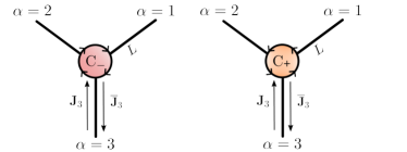
Figure 1: Schematic representation of a junction of spin-1 chains. In the continuum limit, the low-energy modes in each chain $\alpha$ are described by SU(2)₂ currents $\mathsf{\mathbf{J}}_{\alpha}(x)$ and $\bar{\mathsf{\mathbf{J}}}_{\alpha}(x)$. At the chiral fixed points, denoted by C_- and C₊, the currents are perfectly transmitted in the directions represented by the clockwise or counterclockwise loops.

The microscopic interactions in Eq. (2) can be tuned to control the boundary conditions for the low-energy modes at the junction. Two chiral fixed points with opposite chirality, denoted as C₊ and C_-, occur at intermediate values of $J_{\chi}$ and $J^{\prime}$ [32]. They are characterized by the boundary conditions

$$\text{C}_{\pm}:\;\mathbf{J}_{\alpha}(0)=\bar{\mathbf{J}}_{\alpha\pm 1}(0)$$ (14)

At the $\text{C}_{\pm}$ points, the Y junction behaves as an ideal spin circulator [30], in which incoming spin currents are completely transmitted from one chain to the next in rotation, either clockwise or counterclockwise; see Fig. 1. The direction of circulation is controlled by the sign of $J_{\chi}$ at the corresponding chiral fixed point. The chiral boundary conditions can be implemented in terms of Majorana fermions as

$$\text{C}_{\pm}:\;\xi_{\alpha}^{a}(0)=p_{\alpha}\bar{\xi}^{a}_{\alpha\pm 1}(0),$$ (15)

where $p_{\alpha}\in\{+1,-1\}$ can be chosen arbitrarily, manifesting a $\mathbb{Z}_{2}$ gauge freedom in the fermionic representation of Eq. (5). Fixing $p_{\alpha}=+1$, we can glue the fermionic modes in different chains as

$$\text{C}_{\pm}:\;{\xi}_{\alpha}^{a}(x)=\bar{\xi}^{a}_{\alpha\pm 1}(-x).$$ (16)

Thus, we regard the left-moving Majorana fermions as the analytic continuation of the right-moving ones to the domain $x<0$. With this convention, the effective Hamiltonian for a single junction tuned to a chiral fixed point can be cast in the form

$$H_{Y}^{\rm CFP}=-\frac{iv}{2}\sum_{\alpha,a}\int_{-L}^{L}dx\,\bar{\xi}^{a}_{\alpha}\partial_{x}\bar{\xi}^{a}_{\alpha}.$$ (17)

The chiral-fixed-point Hamiltonian is perturbed by one relevant and one marginal boundary operator. These operators are written in terms of the trace of the primary fields at $x=0$:

$$\delta H = \gamma\sum_{\alpha}\text{tr}[\Phi_{\alpha}^{(\frac{1}{2})}(0)]+\lambda\sum_{\alpha}\text{tr}[\Phi_{\alpha}^{(1)}(0)].$$ (18)

The coupling constants $\gamma$ and $\lambda$ vanish when the microscopic parameters $J_{\chi}$ and $J^{\prime}$ are fine tuned to one of the chiral fixed points. The relevant $\gamma$ interaction drives the system towards low-energy fixed points with vanishing spin conductance [32]. The marginal $\lambda$ interaction can be written in terms of Majorana fermions and corresponds to a backscattering process at the junction. These perturbations render the chiral fixed points unstable in the limit $L\to\infty$. However, if the crossover to stable fixed points happens to be slow, as verified numerically for the junction of spin-1/2 chains [30, 31], the chiral fixed point can still govern the physical properties of a junction with finite but very long chains over a wide range of parameters. Moreover, we can cut off the infrared divergence of the relevant perturbation by keeping the chain length finite and imposing boundary conditions at $x=L$ that correspond to constructing a 2D network, as we will discuss in the following.

III Network model with staggered chirality

Consider a honeycomb network constructed by putting together Y junctions of spin-1 chains. To obtain a translationally invariant system, we impose chiral boundary conditions with the same chirality, say the C_- fixed point, on all the junctions marked by yellow dots in Fig. 2. These positions correspond to the $x=0$ end of the spin chains. The choice of the boundary conditions at $x=L$ is crucial. If we impose the same chirality as at $x=0$, we obtain the non-Abelian CSL discussed in Ref. [34]. By contrast, here we assemble a network with staggered chirality in order to obtain a gapless phase. This can be accomplished by tuning the interactions in Eq. (2) among the chains that meet at $x=L$ to the C₊ fixed point. We can write the boundary conditions as

$$\bar{{J}}^{a}_{\alpha,\mathbf{R}}\left(0\right) ={J}^{a}_{\alpha+1,\mathbf{R}}\left(0\right),$$

$$\bar{{J}}^{a}_{\alpha,\mathbf{R}}\left(L\right) ={J}^{a}_{\alpha-1,\mathbf{R}-\bm{\delta}_{\alpha-1}}\left(L\right),$$ (19)

where the lattice vector $\mathbf{R}$ specifies the positions represented as yellow dots in Fig. 2, which form a triangular lattice, and $\bm{\delta}_{\alpha}$ are the next-nearest-neighbor vectors

$$\bm{\delta}_{1} =\sqrt{3}L\left(1,0\right),$$

$$\bm{\delta}_{2} =\sqrt{3}L\left(-1/2,\sqrt{3}/2\right),$$

$$\bm{\delta}_{3} =\sqrt{3}L\left(-1/2,-\sqrt{3}/2\right).$$ (20)

In terms of the Majorana fermions, the chiral boundary conditions in Eq. (19) can be expressed as

$$\bar{\xi}^{a}_{\alpha,\mathbf{R}}\left(0\right) =p_{\alpha,\mathbf{R}}\,\xi^{a}_{\alpha+1,\mathbf{R}}\left(0\right),$$

$$\bar{\xi}^{a}_{\alpha,\mathbf{R}}\left(L\right) =p_{\alpha,\mathbf{R}}\,\xi^{a}_{\alpha-1,\mathbf{R}-\bm{\delta}_{\alpha-1}}\left(L\right),$$ (21)

with $p_{\alpha,\mathbf{R}}\in\{+1,-1\}$. Here we will fix a uniform sign $p_{\alpha,\mathbf{R}}=+1$ $\forall\,\alpha,\mathbf{R}$, but will reexamine this choice later when we discuss the $\mathbb{Z}_{2}$ gauge structure of the resulting 2D phase.

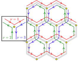
Figure 2: Network of junctions at the chiral fixed point. Inside the box, we represent the unit cell specifying the direction of propagation of the three Majoranas chiral modes. The origin of the triskelion unit cell is represented by the yellow dots, where we have $s=0$.

With this choice of boundary conditions, the network model describes three sets of decoupled chiral 1D modes running along the zigzags of the honeycomb lattice. The three directions of propagation are schematically represented by red, green and blue lines in Fig. 2. These modes are related to each other by the $\mathbb{Z}_{3}$ symmetry that combines a C₃ lattice rotation with $\alpha\mapsto\alpha+1$. To specify positions in this network, we use the coordinates $(\nu,\mathbf{R},s)$, where $\nu=1,\,2,\,3$ labels the direction of propagation (red, green and blue, respectively), $\mathbf{R}$ is the center of the unit cell shown in the inset in Fig. 2, and $s\in[-L,L]$ is a continuous coordinate within the unit cell, with $s=0$ at the center of the unit cell and $s=\pm L$ at the far ends of the chains. In this notation, the Majorana fields obey the relation

$$\bar{\xi}^{a}_{\nu,\mathbf{R}-\bm{\delta}_{\nu}}(s+2L)=\bar{\xi}^{a}_{\nu,\mathbf{R}}(s).$$ (22)

The chiral fixed point Hamiltonian can be written as

$$H_{0} =\frac{v}{2}\sum_{a,\nu}\sum_{\mathbf{R}}\int_{-L}^{L}ds\,\bar{\xi}^{a}_{\nu,\mathbf{R}}\left(s\right)(-i\partial_{s})\bar{\xi}^{a}_{\nu,\mathbf{R}}\left(s\right).$$ (23)

As a consequence of the SU(2) symmetry, the Majorana fermions are degenerate with respect to spin index $a$. It is convenient to single out the $z$ spin direction and define a complex fermion by combining two Majoranas:

$$\bar{\psi}_{\nu,\mathbf{R}}(s) =\frac{1}{\sqrt{2}}\left[\bar{\xi}^{x}_{\nu,\mathbf{R}}(s)+i\bar{\xi}^{y}_{\nu,\mathbf{R}}(s)\right],$$ (24)

with $\{\bar{\psi}^{\phantom{\dagger}}_{\nu,\mathbf{R}}(s),\bar{\psi}^{\dagger}_{\nu^{\prime},\mathbf{R}^{\prime}}(s^{\prime})\}=\delta_{\nu\nu^{\prime}}\delta_{\mathbf{R},\mathbf{R}^{\prime}}\delta(s-s^{\prime})$. We can then write $H_{0}=H_{0}^{xy}+H_{0}^{z}$, with

$$H_{0}^{xy} = v\sum_{\nu,\mathbf{R}}\int_{-L}^{L}ds\,\bar{\psi}^{\dagger}_{\nu,\mathbf{R}}\left(s\right)(-i\partial_{s})\bar{\psi}_{\nu,\mathbf{R}}\left(s\right),$$ (25)

$$H_{0}^{z} = \frac{v}{2}\sum_{\nu,\mathbf{R}}\int_{-L}^{L}ds\,\bar{\xi}^{z}_{\nu,\mathbf{R}}\left(s\right)(-i\partial_{s})\bar{\xi}^{z}_{\nu,\mathbf{R}}\left(s\right).$$ (26)

Hereafter we focus on the spectrum of the complex fermion, but we should keep in mind that the theory also contains the Majorana fermion $\bar{\xi}^{z}$ with the same dispersion relation but half the number of modes.

The quadratic Hamiltonian in Eq. (25) can be diagonalized straightforwardly. We use the mode expansion

$$\bar{\psi}_{\nu,\mathbf{R}}\left(s\right) =\frac{1}{\sqrt{2\mathcal{N}L}}\sum_{\mathbf{k}\in\text{BZ}}\sum_{n\in\mathbb{Z}}e^{i\left[\mathbf{k}\cdot\mathbf{R}+Q_{\nu,n}\left(\mathbf{k}\right)s\right]}\bar{\psi}_{\nu,n}\left(\mathbf{k}\right),$$ (27)

where $\mathcal{N}$ is the number of unit cells and BZ stands for the first Brillouin zone. The auxiliary function $Q_{\nu,n}\left(\mathbf{k}\right)$ is defined as

$$Q_{\nu,n}\left(\mathbf{k}\right)=\frac{\mathbf{k}\cdot\bm{\delta}_{\nu}+2\pi n}{2L},\quad n\in\mathbb{Z}\,,$$ (28)

and obeys $Q_{\nu,\,-n}(-\mathbf{k})=-Q_{\nu,\,n}(\mathbf{k})$. This function is important to ensure the relation $\bar{\psi}_{\nu,\,\mathbf{R}-\mathbf{\delta}_{\nu}}(s+2L)=\bar{\psi}_{\nu,\,\mathbf{R}}(s)$. The Hamiltonian in momentum space can be written as

$$H^{xy}_{0}=\sum_{\nu=1}^{3}\sum_{\mathbf{k}\in\text{BZ}}\sum_{n\in\mathbb{Z}}\mathcal{E}_{\nu,n}(\mathbf{k})\bar{\psi}^{\dagger}_{\nu,n}(\mathbf{k})\bar{\psi}_{\nu,n}(\mathbf{k}),$$ (29)

where

$$\mathcal{E}_{\nu,n}(\mathbf{k})=vQ_{\nu,n}(\mathbf{k})$$ (30)

is the fermion dispersion relation with $n\in\mathbb{Z}$ denoting a band index. It follows from the definition of $Q_{\nu,n}(\mathbf{k})$ that shifting the momentum by a reciprocal lattice vector, $\mathbf{k}\mapsto\mathbf{k}+\mathbf{G}$ with $\mathbf{G}\cdot\bm{\delta}_{\nu}=2\pi\ell$ and $\ell\in\mathbb{Z}$, corresponds to shifting the band index $n\mapsto n+\ell$. Due to the continuum of states inside the unit cell, the spectrum of $H^{xy}_{0}$ exhibits an infinite number of positive- and negative-energy bands. The ground state is a Fermi sea in which all negative-energy state states are occupied. We stress that this field theory approach is aimed at describing the low-energy properties of the network. The low-energy bands correspond to $n=0$ and have the dispersion relation

$$\mathcal{E}_{\nu,0}(\mathbf{k})=\frac{\sqrt{3}}{2}v\mathbf{k}\cdot\hat{\mathbf{e}}_{\nu},$$ (31)

where $\hat{\mathbf{e}}_{\nu}=\bm{\delta}_{\nu}/(\sqrt{3}L)$ are unit vectors. There are three low-energy bands that disperse along the directions of propagation of the chiral 1D modes. The spectrum is gapless along three intersecting straight lines in reciprocal space given by $\mathbf{k}\cdot\hat{\mathbf{e}}_{\nu}=0$.

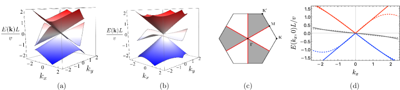
Figure 3: Dispersion relation of fermionic excitations in the network model, see Eq. (37), for two values of the coupling constant of the backscattering operator: (a) $\lambda/v=0.2$; (b) $\lambda/v=0.8$. Panel (c) shows the Fermi surface of the middle band (red lines), with occupied states corresponding to the shaded regions. The primitive reciprocal lattice vectors are $\mathbf{b}_{1}=\left(\frac{2\pi}{\sqrt{3}L},\frac{2\pi}{3L}\right)$ and $\mathbf{b}_{2}=\left(0,-\frac{4\pi}{3L}\right)$. In panel (d), the dispersion for $\lambda/v=0.8$ (solid lines) is compared with the tight-binding model of Eq. (40) with $t_{1}=0.78v/L$ and $t_{3}=1.09v/L$ (dashed lines). Here we set $E_{\rm max}=v/L$ as the energy cutoff for the fitted data.

The solution of the chiral-fixed-point Hamiltonian in terms of decoupled 1D modes has a direct impact on the spin correlation. Let $\mathbf{S}_{j,\alpha,\mathbf{R}}$ denote the spin operator at site $j$ of chain $\alpha$ of the junction centered at $\mathbf{R}$. Given the chain index $\alpha$, the two chiral modes that run through this chain propagate along the directions labeled as $\nu=\alpha$ and $\nu=\alpha-1$; see Figs. 1 and 2. At the chiral fixed point, two spins separated by a distance $r>L$ are correlated only if there is a chiral mode that connects them. This condition requires that the second point be located at a unit cell given by $\mathbf{R}^{\prime}=\mathbf{R}+m\bm{\delta}_{\alpha}$ or $\mathbf{R}^{\prime}=\mathbf{R}+m\bm{\delta}_{\alpha-1}$ with $m\in\mathbb{Z}$. We can then compute the correlation using the representation of the spin operator in Eq. (13) and the operator product expansion (OPE) of the SU(2)₂ currents [35, 41]

$$\bar{{J}}^{a}(\bar{z})\bar{{J}}^{b}(\bar{z}^{\prime})\sim\frac{1}{4\pi^{2}}\frac{\delta^{ab}}{(\bar{z}-\bar{z}^{\prime})^{2}}+i\epsilon^{abc}\frac{\bar{{J}}^{c}_{\alpha}(\bar{z}^{\prime})}{2\pi(\bar{z}-\bar{z}^{\prime})},$$ (32)

where $\bar{z}=v\tau-ix$ is the anti-holomorphic coordinate in Euclidean spacetime. We obtain

$$\langle{S}^{z}_{j,\alpha,\mathbf{R}}{S}^{z}_{j^{\prime},\alpha^{\prime},\mathbf{R}^{\prime}}\rangle\sim-\frac{\delta_{\mathbf{R}^{\prime},\mathbf{R}+m\bm{\delta}_{\alpha}}+\delta_{\mathbf{R}^{\prime},\mathbf{R}+m\bm{\delta}_{\alpha-1}}}{4\pi^{2}(s^{\prime}-s+2mL)^{2}},$$ (33)

where on the right-hand side $s,s^{\prime}\in[-L,L]$ are coordinates within the unit cells corresponding to the sites $(j,\alpha,\mathbf{R})$ and $(j^{\prime},\alpha^{\prime},\mathbf{R}^{\prime})$, respectively, for the chiral model that connects these two points. Thus, the correlation is spatially anisotropic and decays as a power law with the distance along the special directions set by the vectors $\bm{\delta}_{\alpha}$. Remarkably, the staggered part of the correlation vanishes because the spin-1/2 primary field acts nontrivially on both chiral sectors of a given chain, and two points separated by a distance $r>L$ cannot share both chiral modes. The same behavior was obtained within a different coupled-wire construction for a model with staggered chirality on the extended kagome lattice [27].

IV Perturbations to the chiral fixed point

So far we have explored the physics of the network model when the microscopic interactions are tuned to the chiral fixed points. An immediate question concerns what happens in the presence of perturbations associated with deviations from the chiral fixed point. As discussed in Sec. II, for a single junction there are only two non-irrelevant interaction terms given by Eq. (18). We now analyze the effects of these perturbations on the excitation spectrum of the network. We start with the marginal operator, which involves the spin-1 field and can be treated exactly, and then proceed to the analysis of the operator that involves the spin-1/2 field.

IV.1 Spin-1 perturbation: backscattering of Majorana fermions

Let us consider the second term in Eq. (18). Using the fermionic representation and imposing either C₊ or C_- chiral boundary conditions, we can write this term as

$$\delta H^{(\text{C}_{\pm})}_{\lambda}=i\lambda\sum_{a,\alpha}\bar{\xi}^{a}_{\alpha\pm 1}(0)\bar{\xi}^{a}_{\alpha}(0).$$ (34)

This operator corresponds to a backscattering process that hybridizes the chiral modes at $x=0$. For a single junction, this marginal perturbation defines a critical line in the boundary phase diagram where the spin conductance tensor can be calculated exactly [32]. When transported to the network with staggered chirality, the perturbation becomes

$$H_{\lambda}=-i\lambda\sum_{\eta=0,1}\sum_{a,\nu}\sum_{\mathbf{R}}(-1)^{\eta}\bar{\xi}^{a}_{\nu+1,\mathbf{R}}(\eta L)\bar{\xi}^{a}_{\nu,\mathbf{R}-\eta\bm{\delta}_{\nu}}(\eta L).$$ (35)

Importantly, the sign of the backscattering amplitude alternates between $s=0$ and $s=L$. This property is related to a mirror symmetry of the network model with staggered chirality. Consider the reflection with respect to a horizontal line that runs through the center of a hexagon in Fig. 2. We define the vectors $\mathbf{w}_{1}=L(\frac{\sqrt{3}}{2},\frac{1}{2})$, $\mathbf{w}_{2}=L(\frac{\sqrt{3}}{2},-\frac{1}{2})$ and $\mathbf{w}_{3}=L(0,-1)$, such that $\bm{\delta}_{\alpha}=\mathbf{w}_{\alpha}-\mathbf{w}_{\alpha+1}$. The mirror symmetry is implemented as

$${\bar{\xi}}_{1,\mathbf{R}}(s) \mapsto\begin{cases}\bar{\xi}_{1,\tilde{\mathbf{R}}-\mathbf{w}_{2}}(s-L)&\mbox{if $s\in(0,L)$},\\ \bar{\xi}_{1,\tilde{\mathbf{R}}-\mathbf{w}_{1}}(s+L)&\mbox{if $s\in(-L,0)$},\end{cases}$$

$${\bar{\xi}}_{2,\mathbf{R}}(s) \mapsto\begin{cases}\bar{\xi}_{3,\tilde{\mathbf{R}}-\mathbf{w}_{1}}(s-L)&\mbox{if $s\in(0,L)$},\\ \bar{\xi}_{3,\tilde{\mathbf{R}}-\mathbf{w}_{3}}(s+L)&\mbox{if $s\in(-L,0)$},\end{cases}$$

$${\bar{\xi}}_{3,\mathbf{R}}(s) \mapsto\begin{cases}\bar{\xi}_{2,\tilde{\mathbf{R}}-\mathbf{w}_{3}}(s-L)&\mbox{if $s\in(0,L)$},\\ \bar{\xi}_{2,\tilde{\mathbf{R}}-\mathbf{w}_{2}}(s+L)&\mbox{if $s\in(-L,0)$},\end{cases}$$ (36)

where $\tilde{\mathbf{R}}$ stands for the unit cell position after the reflection. It is straightforward to check that the operator in Eq. (35) is invariant under this transformation, but only if the relative minus sign is properly taken into account. This symmetry should not be confused with $\mathcal{P}$ defined in Eq. (3), which refers to a reflection about a vertical line through the center of a hexagon. The latter inverts the direction of propagation of all chiral modes, but it can be combined with time reversal to yield the $\mathcal{P}\mathcal{T}$ symmetry of the network model.

The effective Hamiltonian including the marginal perturbation is quadratic in the Majorana fermions and can be diagonalized exactly. Once again, we focus on the contribution from the complex fermion in Eq. (24) and use the mode expansion in Eq. (27). The leading effect of the backscattering term is to generate avoided level crossings of nearly degenerate states, opening gaps between bands in close analogy with the band structure of electrons in a weak periodic potential [44]. Truncating the spectrum to keep only the low-energy bands with index $n=0$, we can write

$$H^{xy}=H_{0}^{xy}+H_{\lambda}^{xy}=\sum_{\mathbf{k}}\Psi^{\dagger}(\mathbf{k})\mathcal{H}_{\rm eff}(\mathbf{k})\Psi(\mathbf{k}),$$ (37)

where $\Psi(\mathbf{k})=\left(\bar{\psi}_{1,0}(\mathbf{k}),\bar{\psi}_{2,0}(\mathbf{k}),\bar{\psi}_{3,0}(\mathbf{k})\right)^{\text{T}}$. The Bloch Hamiltonian reads

$$\mathcal{H}_{\text{eff}}(\mathbf{k})=\left(\begin{array}[]{ccc}\mathcal{E}_{1,0}(\mathbf{k})&\Lambda_{12}(\mathbf{k})&\Lambda_{31}^{*}(\mathbf{k})\\ \Lambda_{12}^{*}(\mathbf{k})&\mathcal{E}_{2,0}(\mathbf{k})&\Lambda_{23}(\mathbf{k})\\ \Lambda_{31}(\mathbf{k})&\Lambda_{23}^{*}(\mathbf{k})&\mathcal{E}_{3,0}(\mathbf{k})\end{array}\right),$$ (38)

where the off-diagonal elements are given by

$$\Lambda_{\nu,\nu+1}(\mathbf{k})=\frac{i\lambda}{2L}\left(1-e^{-i\mathbf{k}\cdot\bm{\delta}_{\nu-1}/2}\right).$$ (39)

Note that $\Lambda_{\nu,\nu+1}(\mathbf{k})$ vanishes for $\mathbf{k}\to 0$ as a result of the negative interference between the scattering processes at $x=0$ and $x=L$.

Diagonalizing $\mathcal{H}_{\text{eff}}(\mathbf{k})$, we obtain closed-form but lengthy expression for the dispersion relations of the fermionic bands, denroted as $E_{r}(\mathbf{k})$ with $r=1,2,3$. The result is shown in Fig. 3. The bands have the property $E_{r}(-\mathbf{k})=-E_{4-r}(\mathbf{k})$. In particular, $E_{2}(\mathbf{k})$ transforms into itself under $\mathbf{k}\mapsto-\mathbf{k}$. The gapless lines of this middle band are determined by the zeros of the determinant of $\mathcal{H}_{\text{eff}}(\mathbf{k})$. Using $\sum_{\nu}\bm{\delta}_{\nu}=0$, it is easy to show that the gapless lines occur at $\mathbf{k}\cdot\hat{\mathbf{e}}_{\nu}=0$, which is the same Fermi surface that we obtained for the chiral fixed point. Here it is important that setting $\mathbf{k}\cdot\hat{\mathbf{e}}_{\nu}=0$ implies $\Lambda_{\nu+1,\nu-1}(\mathbf{k})=0$; see Eq. (39). This vanishing of the off-diagonal matrix element can be traced back to the relative minus sign in the backscattering Hamiltonian, and is thus related to the mirror symmetry. The bandwidth of $E_{2}(\mathbf{k})$ decreases as we increase the ratio $\lambda/v$. In addition to the Fermi surface of the middle band, the lower and upper bands touch zero energy with a Dirac cone at the $\Gamma$ point.

A qualitatively similar spectrum has been obtained in parton mean-field descriptions of gapless CSLs on the kagome lattice [27, 14, 15]. Note, however, that the result obtained here does not rely on mean-field approximations because the fractionalization into Majorana fermions is established within the building blocks, namely the critical spin-1 chains. To make the connection with parton mean-field theory more explicit, we can fit the low-energy spectrum of the effective Hamiltonian to a tight-binding model. This approximation is better justified when we increase the coupling constant of the marginal operator so that the band splitting, determined by the off-diagonal matrix elements of order $|\lambda|/L$ in Eq. (39), becomes comparable to the bandwidth $W\sim v/L$ of the unperturbed model.

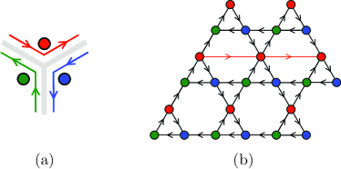
Figure 4: Mapping to a tight-binding model. (a) Each chiral mode ($\nu=1,2,3$ for red, green, and blue, respectively) of the $n=0$ bands is mapped onto a single site. (b) The propagation of the chiral modes can be represented on an extended kagome lattice. The red line indicates the direction of free propagation of the $\nu=1$ mode; cf. Fig. 2. Similarly, the modes $\nu=2,3$ run along the other diagonals of the hexagons. The arrows in the black lines represent the orientation of the links in the backscattering term; see Eq. (40).

The mapping of the network model to a tight-binding model can be visualized as shown in Fig. 4. We represent the chiral modes in the low-energy bands as three sites forming a triangle and assign three Wannier states $|\mathbf{R},\nu\rangle$ to each unit cell. Putting the unit cells together, we naturally obtain a kagome lattice. The free propagation of the chiral modes at the chiral fixed point, see Fig. 2, corresponds to hopping along the diagonals of the hexagons, which connect sites that belong to the same sublattice. The backscattering processes at the junctions are mapped onto hoppings between nearest-neighbor sites, which belong to different sublattices and form the triangles of the kagome lattice. The minimal tight-binding model compatible with the symmetries of the model is

$$H^{xy}_{\rm tb} = \frac{it_{1}}{2}\sum_{\nu,\mathbf{R}}\left[(f^{\dagger}_{\mathbf{R}-\mathbf{a}_{\nu-1},\nu+1}-f^{\dagger}_{\mathbf{R},\nu+1})f^{\phantom{\dagger}}_{\mathbf{R},\nu}-\text{h.c.}\right]$$ (40)

$$+\frac{it_{3}}{2}\sum_{\mathbf{R},\nu}\left(f^{\dagger}_{\mathbf{R}+\mathbf{a}_{\nu},\nu}f^{\phantom{\dagger}}_{\mathbf{R},\nu}-\text{h.c.}\right),$$

where $f_{\mathbf{R},\nu}$, $t_{1}$ and $t_{3}$ are the hopping parameters of order $v/L$ and we set $\mathbf{a}_{\nu}=\bm{\delta}_{\nu}/2$ to match the off-diagonal matrix elements in Eq. (39). As a result, the network model describes a staggered-flux ansatz [11] with first- and third-neighbor links on a kagome lattice. Note that a second-neighbor imaginary hopping $it_{2}$ is forbidden because it would break the reflection symmetry of the network model. We can fit the hopping parameters to reproduce the low-energy spectrum by minimizing the mean square deviation for the dispersion relation in the range $|E_{r}(\mathbf{k})|<E_{\rm max}$ with $E_{\rm max}\sim v/L$; see Fig. 3(d). Importantly, the ratio $t_{1}/t_{3}$ increases with $\lambda/v$ up to $\lambda/v\sim 1$, at which point the middle band becomes approximately flat.

The Majorana Fermi surface governs the low-energy properties of the CSL on the 2D network. For instance, the local dynamical spin correlation behaves as

$$C(\omega) =\int_{-\infty}^{\infty}dt\,e^{i\omega t}\langle S^{z}_{j,\alpha,\mathbf{R}}(t)S^{z}_{j,\alpha,\mathbf{R}}(0)\rangle\sim\omega,$$ (41)

analogous to the local density of states of particle-hole excitations in a Fermi liquid. We can show that the power-law decay of the equal-time spin correlation at distances $r=|\mathbf{r}\cdot\hat{\mathbf{e}}_{\nu}|\gg L$ predicted in Eq. (33) remains valid in the presence of the backscattering operator because the Fermi surface still has the form of straight lines [27]. This is a slower decay than the $1/r^{3}$ behavior expected for a 2D Fermi surface with nonzero curvature [45]. In addition, quantum spin liquids with a Fermi surface of fractional excitations are characterized by a logarithmic violation of the area law for the entaglement entropy [46, 47]. In two dimensions, the entanglement entropy $S_{E}$ of a subsystem of linear size $\mathcal{L}$ in the gapless CSL scales as $S_{E}\sim\mathcal{L}\ln\mathcal{L}$. In this network construction, the logarithmic correction of the 2D phase is directly connected to the entanglement entropy of the chiral 1D modes. The simple argument [27] is that the number of 1D modes that crosses the boundary of the subsystem with linear size $\mathcal{L}\gg L$ is proportional to $\mathcal{L}$, and each mode contributes to the entanglement entropy with $S_{E}^{\rm 1D}\sim c\ln\mathcal{L}$, where $c$ is the central charge of the CFT [48].

A remark about the nomenclature is in order. We refer to this CSL state as “Majorana Fermi surface” rather than “spinon Fermi surface” because we reserve the term “spinon” for excitations that carry spin $1/2$, whereas the gapless Majorana fermions carry spin $1$ [49, 50]. In the next section we will discuss the properties of the spin-1/2 excitations in the network model and show that they are related to gapped visons.

IV.2 Spin-1/2 perturbation: visons

We now turn to the perturbation described by the first term in Eq. (18). In the network model, we define

$$H_{\gamma}=\gamma\sum_{\eta=0,1}\sum_{\alpha}\sum_{\mathbf{R}}\sigma_{\alpha,\mathbf{R}}^{1}(\eta L)\sigma_{\alpha,\mathbf{R}}^{2}(\eta L)\sigma_{\alpha,\mathbf{R}}^{3}(\eta L),$$ (42)

where we used the representation in Eq. (8). Unlike the other terms of the effective Hamiltonian we have discussed so far, $H_{\gamma}$ cannot be written as a local operator in terms of Majorana fermions. In the network with uniform chirality, the same operator has been shown to create visons that bind Majorana zero modes and behave as non-Abelian spinons [34]. Thus, we anticipate that this perturbation also creates visons in the gapless CSL, and it is important to check that these excitations are gapped and do not proliferate in the ground state.

First, we note that the Majorana fermions become interacting in the presence of the $\gamma$ perturbation. To see this, we use the OPE of the order operator in the Ising CFT, represented by the fusion rule [41]

$$\sigma\times\sigma=\mathbb{1}+\varepsilon,$$ (43)

where $\mathbb{1}$ denotes the identity operator. We then treat $H_{\lambda}$ within second-order perturbation theory, applying the OPE to the $\sigma$ fields in the independent spin sectors labeled by $a=1,2,3$. Integrating out high-energy modes, we generate a term linear in $\varepsilon_{\alpha}^{a}$, which amounts to a renormalization of the backscattering amplitude $\lambda$. In addition, we obtain a quadratic term in the energy operator the form

$$H_{\rm int}=g\sum_{\mathbf{R}}\sum_{\eta=0,1}\sum_{a,\alpha}\sum_{\mathbf{R}}\varepsilon_{\alpha,\mathbf{R}}^{a}(\eta L)\varepsilon_{\alpha,\mathbf{R}}^{a+1}(\eta L),$$ (44)

which is a fermion-fermion interaction with coupling constant $g\sim\gamma^{2}$. Based on general arguments for $\mathbb{Z}_{2}$ quantum spin liquids with broken time reversal and reflection symmetries [9, 18, 20], we expect the Majorana Fermi surface in the network model to be robust against this short-range interaction in the small-$\gamma$ limit.

Beyond the approximation of integrating out the $\sigma$ operators, the $\gamma$ interaction must be related to an emergent $\mathbb{Z}_{2}$ gauge field. Let us revisit the $\mathbb{Z}_{2}$ gauge degree of freedom alluded to in Eq. (21). The variable $p_{\alpha,\mathbf{R}}\in\{+1,-1\}$ can be interpreted in terms of the phase shift that the Majorana fermion picks up when tunneling from one chain to the next according to the chiral boundary conditions. At the chiral fixed point, a sign change in $p_{\alpha,\mathbf{R}}$ at any junction can be gauged away since the chiral modes are defined on open lines that extend out to infinity. However, once we turn on the backscattering operator, the Majorana fermions acquire a 2D dispersion, which means they can then move around in closed paths and feel the physical effects of a gauge-invariant $\mathbb{Z}_{2}$ flux.

When we set $p_{\alpha,\mathbf{R}}=+1$ $\forall\alpha,\mathbf{R}$ in the effective Hamiltonian, we assumed that the uniform gauge configuration describes the sector of the Hilbert space that contains the ground state. For consistency, we must check that this configuration is at least locally stable in the sense that flipping the sign of $p_{\alpha,\mathbf{R}}$ at a given junction costs energy. The action of the operator in Eq. (42) has precisely this effect because $\sigma$ acts as a twist field that changes the boundary conditions for the Majorana fermions [51, 34]. In fact, Eq. (11) implies that the fermions pick up a minus sign when they go around the point where $\sigma$ is applied.

To estimate the energy of the gauge-field excitations, we turn to the effective tight-binding model in Eq. (40). We implement the $\mathbb{Z}_{2}$ gauge degree of freedom by rewriting the Hamiltonian as

$$H^{xy}_{\rm tb}=\frac{i}{2}\sum_{ij}u_{ij}t_{ij}f^{\dagger}_{i}f^{\phantom{\dagger}}_{j},$$ (45)

where $t_{ij}=t_{1}$ for first-neighbor links, $t_{ij}=t_{3}$ for third-neighbor links, and $t_{ij}=0$ otherwise. Here $u_{ij}\in\{+1,-1\}$ denotes an Ising link variable obeying the relation $u_{ji}=-u_{ij}$. In the proposed ground state, we fix the positive orientation of the links with nonzero $u_{ij}$ as represented by the arrows in Fig. 4(b). The gauge-invariant $\mathbb{Z}_{2}$ flux can be defined from the product of $u_{ij}$ around the plaquettes of the kagome lattice [16, 17, 18]. The effect of the $\gamma$ perturbation in Eq. (42) is mapped onto flipping the sign of the variable $u_{ij}$ that corresponds to a path on the network that contains the point where the order operator $\sigma$ is applied. As a result, the quantum fluctuations of $u_{ij}$ create pairs of visons on neighboring plaquettes that share the link $(i,j)$. For $\gamma\neq 0$, the $\mathbb{Z}_{2}$ gauge field becomes a dynamical degree of freedom. The situation here is analogous to the effect of integrability-breaking interactions in the Kitaev spin liquid [52, 53].

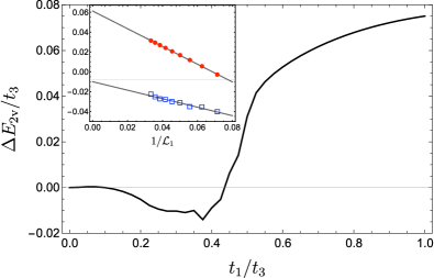
Figure 5: Energy of a pair of adjacent vortices in the effective tight-binding model of Eq. (45). The energy is calculated by extrapolating the result for finite-size systems to the thermodynamic limit, as shown in the inset for $t_{1}/t_{3}=0.35$ (blue squares) and $t_{1}/t_{3}=0.7$ (red circles).

We consider a state with localized visons created by reversing the sign of a single link variable $u_{ij}$ on a triangle of the kagome lattice. Since this gauge configuration breaks translational invariance, we calculate the energy of this state numerically by diagonalizing the tight-binding Hamiltonian on a finite lattice with size $\mathcal{L}_{1}\times\mathcal{L}_{2}$ along the directions of the vectors $\mathbf{a}_{1}$ and $\mathbf{a}_{2}$ with periodic boundary conditions. This calculation is performed for system sizes up to $\mathcal{L}_{1}=\mathcal{L}_{2}=30$. By subtracting the energy of the vortex-free ground state and extrapolating the result to $\mathcal{L}_{1}\to\infty$, we obtain an estimate for the energy $E_{\rm 2v}$ of the two-vortex excitation. Since the $\gamma$ perturbation acts on the $\bar{\xi}^{z}$ Majorana fermion as well as on $\bar{\xi}^{x}$ and $\bar{\xi}^{y}$, we multiply the energy calculated from $H_{\rm tb}^{xy}$ by a factor $3/2$ to account for the contribution from all three spin flavors. The result is shown in Fig. 5. We find that the finite-size effects are stronger for small $t_{1}/t_{3}$, but it is clear that the energy $E_{\rm 2v}$ starts off negative and becomes positive for larger $t_{1}/t_{3}$, within the range $\lambda<v$; cf. Fig. 3. This result indicates that the stability of the Majorana Fermi surface state against vison excitations requires moving away from the chiral fixed point of decoupled 1D modes and towards a 2D regime with a significant backscattering amplitude. We have also considered the case $t_{1}<0$, which can accessed by reversing the sign of $\lambda$, but found that $E_{\rm 2v}$ is always negative in this case.

Besides creating vison pairs, the $\gamma$ interaction can make the visons mobile, lowering their energy. At fixed $\lambda$, we expect a quantum phase transition out of the Majorana Fermi surface state as we increase $\gamma$ to the point where visons condense. To understand the conditions on the critical $\gamma$, recall that this operator is relevant and increases under the RG flow in the 1D theory. Assuming that the RG flow is cut off at the energy scale $W\sim v/L$ set by the bandwidth of the 2D network model, we replace the bare coupling constant $\gamma$ by the effective coupling $\gamma^{*}(L)\sim\gamma\,L^{1-\Delta}$, where $\Delta=3/8$ is the scaling dimension of the spin-1/2 matrix field. The transition must happen when the effective vison bandwidth generated by $\gamma^{*}$ approaches the gap obtained for $\gamma=0$. Thus, we expect the gapless CSL phase to extend over the regime

$$\frac{|\gamma^{*}(L)|}{L}\lesssim\frac{v}{L}\Rightarrow\frac{1}{L}\gtrsim\left(\frac{|\gamma|}{v}\right)^{8/5}.$$ (46)

For fixed $\gamma\neq 0$, the gapless CSL becomes unstable in the limit $L\to\infty$, reflecting the instability of the chiral fixed point for a single junction of infinitely long chains [32]. On the other hand, this analysis suggests that, even though we started in the limit of long chains with low-energy excitations described by a CFT, the gapless CSL phase actually becomes more stable if we push the result towards the physically relevant regime of short chains, with fewer sites in the unit cell.

Let us also comment on the behavior of the staggered part of the spin correlation in the network model. In contrast with the result for the chiral fixed point discussed in Sec. III, the staggered part of the correlation does not vanish in the generic Majorana Fermi surface state with nonzero $\lambda$ and $\gamma$. However, since the staggered magnetization involves the spin-1/2 primary field and creates visons, this correlation must decay exponentially with a length scale set by the vison gap. The same can be said about the correlation for the dimerization operator, which is represented by the trace of the spin-1/2 field [32]. By contrast, recall that the uniform part of the spin correlation, which only involves gapless fermion excitations, decays as a power law according to Eq. (33).

V Magnetic field response

In this section, we analyze the effects of an external magnetic field on the Majorana Fermi surface state. The Zeeman term for a magnetic field applied along the $z$ spin direction is

$$H_{\text{Z}}=-BS^{z}_{\rm total}=-B\sum_{j,\alpha,\mathbf{R}}S^{z}_{j,\alpha,\mathbf{R}}.$$ (47)

The total magnetization $S^{z}_{\rm total}$ can be written in terms of the integral of the chiral currents in Eq. (13). Using the representation in Eq. (5), we obtain

$$H_{\text{Z}}=iB\sum_{\mathbf{R}}\sum_{\nu}\int_{-L}^{L}ds\,\bar{\xi}^{x}_{\nu,\mathbf{R}}(s)\bar{\xi}^{y}_{\nu,\mathbf{R}}(s).$$ (48)

Since the magnetic field only couples to $\bar{\xi}^{x}$ and $\bar{\xi}^{y}$, the dispersion relation of the Majorana fermion $\bar{\xi}^{z}$ remains unchanged. In terms of the complex fermion in Eq. (24), the Hamiltonian reads (up to a constant)

$$H_{\text{Z}}=B\sum_{\mathbf{R}}\sum_{\nu}\int_{-L}^{L}ds\,\bar{\psi}^{\dagger}_{\nu,\mathbf{R}}(s)\bar{\psi}_{\nu,\mathbf{R}}(s).$$ (49)

Thus, the Zeeman term is equivalent to a chemical potential for the complex fermion. The analogous term in the tight-binding model of Eq. (40) is

$$H_{\text{Z}}=B\sum_{\nu,\mathbf{R}}f^{\dagger}_{\nu,\mathbf{R}}f^{\phantom{\dagger}}_{\nu,\mathbf{R}}.$$ (50)

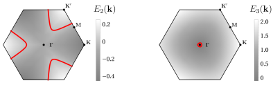
Figure 6: Energy contour plots of the bands $E_{2}(\mathbf{k})$ (left) and $E_{3}(\mathbf{k})$ (right) for $\lambda/v=0.8$ and $B=-0.1v/L$. The red lines correspond to the Fermi surface.

Since the Zeeman term only shifts the Fermi level for the complex fermion, the spectrum remains gapless for $B\neq 0$. However, the symmetry $E_{r}(-\mathbf{k})=-E_{4-r}(\mathbf{k})$ is broken and the Fermi surface changes significantly; see Fig. 6. The Fermi lines of the middle band $E_{2}(\mathbf{k})$ become curves and no longer cross at the $\Gamma$ point. In addition, for $B<0$ the upper band $E_{3}(\mathbf{k})$ crosses the Fermi level and contributes to the Fermi surface with a small pocket around the $\Gamma$ point. Due to the nonzero curvature of the Fermi surface, in the presence of the Zeeman field the equal-time spin correlation for the $S^{z}$ component decays as $1/r^{3}$ [45]. In addition, the magnetic field affects the low-energy single-particle density of states (DOS), $\rho(E)=\frac{1}{\mathcal{N}}\sum_{\mathbf{k},r}\delta(E_{r}(\mathbf{k})-E)$. At zero field, we have $\rho(-E)=\rho(E)$, and the DOS has a peak at $E=0$. Since the Zeeman term shifts the Fermi level to $E_{F}=-B$, the low-energy DOS decreases when we turn on the magnetic field. This results, in particular, in a suppression of the specific heat $c_{V}(T)\propto\rho(E_{F})T$.

VI Conclusions

We presented an analytic approach to study a 2D gapless phase in a network built out of junctions of spin-1 chains. Gapless phases are hard to explore beyond the approximations of parton mean-field theory or even within coupled-wire constructions that assume strong-coupling fixed points at low energies. By imposing chiral boundary conditions with staggered chirality on the network, we showed that our effective model gives rise to a phase that shares several low-energy properties with gapless CSLs found in mean-field approaches on the kagome lattice [54, 14, 15]. For instance, this gapless CSL is characterized by a power-law-decaying spin correlations and a low-energy density of states dominated by a Fermi surface of spin-1 Majorana fermion excitations.

The main advantage of this approach is that fractionalization arises naturally within the effective field theory description of the spin chains. The challenge is to verify that the resulting 2D phase remains stable against perturbations that are formally relevant at the chiral fixed point of the 1D theory. As a key ingredient, the marginal operator associated with backscattering of Majorana fermions at the junctions provides a way to tune the excitation spectrum along a line of fixed points. Moving along this line to reach the 2D regime, we were able to associate the spin-1/2 excitations with gapped visons and to analyze the conditions for stabilizing the gapless CSL phase.

Gapless quantum spin liquid states have been proposed for spin-1 systems with bilinear and biquadratic interactions on the triangular lattice, mainly motivated by the material Ba₃NiSb₂O₉ [55, 56, 57]. Extrapolating our results to the limit of short chains, we expect that the gapless CSL identified here should be found in spin-1 models on the kagome and star lattices with three-spin interactions. This model could be studied using the same numerical methods that have been applied to the spin-1/2 case [14, 15].

Among the directions to be explored in future work, it would be interesting to numerically map out the boundary phase diagram of the junction of spin-1 chains, as done for spin-1/2 chains [30, 31]. An accurate quantitative estimate of the location of the chiral fixed point and the critical line defined by the marginal operator would provide guidance for the parameter regime where the CSL phase can be found. Moreover, a natural question is whether there are other SU$(N)_{k}$ WZNW models that allow the construction of 2D gapless phases. A lesson from this work is that a good starting point is to search for marginal boundary operators in the operator content of the CFT. Finally, the generalization to other tricoordinated networks and higher spatial dimensions can lead to even more exotic states.

VII Acknowledgments

The authors are grateful to Vanuildo de Carvalho and Hernan Xavier for discussions. This work was supported by a grant from the Simons Foundation (1023171, W.B.F., R.G.P.) and by the Brazilian funding agency CNPq (F.G.O., R.G.P.). W.B.F. acknowledges FUNPEC under grant 182022/1707. Research at IIP-UFRN is supported by Brazilian ministries MEC and MCTI.

References

- Sachdev [2023] S. Sachdev, Quantum Phases of Matter (Cambridge University Press, 2023).
- Savary and Balents [2016] L. Savary and L. Balents, Rep. Prog. Phys. 80, 016502 (2016).
- Knolle and Moessner [2019] J. Knolle and R. Moessner, Annu. Rev. Condens. Matter Phys. 10, 451 (2019).
- Broholm et al. [2020] C. Broholm, R. J. Cava, S. A. Kivelson, D. G. Nocera, M. R. Norman, and T. Senthil, Science 367, eaay0668 (2020).
- Lee et al. [2006] P. A. Lee, N. Nagaosa, and X.-G. Wen, Rev. Mod. Phys. 78, 17 (2006).
- Wen [2002] X.-G. Wen, Phys. Rev. B 65, 165113 (2002).
- Hermele et al. [2004] M. Hermele, T. Senthil, M. P. A. Fisher, P. A. Lee, N. Nagaosa, and X.-G. Wen, Phys. Rev. B 70, 214437 (2004).
- Lee [2008] S.-S. Lee, Phys. Rev. B 78, 085129 (2008).
- Barkeshli et al. [2013] M. Barkeshli, H. Yao, and S. A. Kivelson, Phys. Rev. B 87, 140402 (2013).
- Senthil and Fisher [2000] T. Senthil and M. P. A. Fisher, Phys. Rev. B 62, 7850 (2000).
- Bieri et al. [2016] S. Bieri, C. Lhuillier, and L. Messio, Phys. Rev. B 93, 094437 (2016).
- Metlitski et al. [2015] M. A. Metlitski, D. F. Mross, S. Sachdev, and T. Senthil, Phys. Rev. B 91, 115111 (2015).
- Gong et al. [2019] S.-S. Gong, W. Zheng, M. Lee, Y.-M. Lu, and D. N. Sheng, Phys. Rev. B 100, 241111 (2019).
- Bauer et al. [2019] B. Bauer, B. P. Keller, S. Trebst, and A. W. W. Ludwig, Phys. Rev. B 99, 035155 (2019).
- Oliviero et al. [2022] F. Oliviero, J. A. Sobral, E. C. Andrade, and R. G. Pereira, SciPost Phys. 13, 050 (2022).
- Chua et al. [2011] V. Chua, H. Yao, and G. A. Fiete, Phys. Rev. B 83, 180412 (2011).
- Lai and Motrunich [2011a] H.-H. Lai and O. I. Motrunich, Phys. Rev. B 83, 155104 (2011a).
- Lai and Motrunich [2011b] H.-H. Lai and O. I. Motrunich, Phys. Rev. B 84, 085141 (2011b).
- Hermanns and Trebst [2014] M. Hermanns and S. Trebst, Phys. Rev. B 89, 235102 (2014).
- Chari et al. [2021] R. Chari, R. Moessner, and J. G. Rau, Phys. Rev. B 103, 134444 (2021).
- Gorohovsky et al. [2015] G. Gorohovsky, R. G. Pereira, and E. Sela, Phys. Rev. B 91, 245139 (2015).
- Meng et al. [2015] T. Meng, T. Neupert, M. Greiter, and R. Thomale, Phys. Rev. B 91, 241106 (2015).
- Huang et al. [2016] P.-H. Huang, J.-H. Chen, P. R. S. Gomes, T. Neupert, C. Chamon, and C. Mudry, Phys. Rev. B 93, 205123 (2016).
- Patel and Chowdhury [2016] A. A. Patel and D. Chowdhury, Phys. Rev. B 94, 195130 (2016).
- Lecheminant and Tsvelik [2017] P. Lecheminant and A. M. Tsvelik, Phys. Rev. B 95, 140406 (2017).
- Leviatan and Mross [2020] E. Leviatan and D. F. Mross, Phys. Rev. Res. 2, 043437 (2020).
- Pereira and Bieri [2018] R. G. Pereira and S. Bieri, SciPost Phys. 4, 004 (2018).
- Slagle et al. [2022] K. Slagle, Y. Liu, D. Aasen, H. Pichler, R. S. K. Mong, X. Chen, M. Endres, and J. Alicea, Phys. Rev. B 106, 115122 (2022).
- Oshikawa et al. [2006] M. Oshikawa, C. Chamon, and I. Affleck, J. Stat. Mech.: Theory Exp. 2006 (02), P02008.
- Buccheri et al. [2018] F. Buccheri, R. Egger, R. G. Pereira, and F. B. Ramos, Phys. Rev. B 97, 220402(R) (2018).
- Buccheri et al. [2019] F. Buccheri, R. Egger, R. G. Pereira, and F. B. Ramos, Nuclear Physics B 941, 794 (2019).
- Xavier and Pereira [2022] H. B. Xavier and R. G. Pereira, Phys. Rev. B 106, 064429 (2022).
- Ferraz et al. [2019] G. Ferraz, F. B. Ramos, R. Egger, and R. G. Pereira, Phys. Rev. Lett. 123, 137202 (2019).
- Xavier et al. [2023] H. B. Xavier, C. Chamon, and R. G. Pereira, SciPost Phys. 14, 105 (2023).
- Gogolin et al. [2004] A. O. Gogolin, A. A. Nersesyan, and A. M. Tsvelik, Bosonization and strongly correlated systems (Cambridge University Press, 2004).
- Tsvelik [1990] A. M. Tsvelik, Phys. Rev. B 42, 10499 (1990).
- Allen and Sénéchal [2000] D. Allen and D. Sénéchal, Phys. Rev. B 61, 12134 (2000).
- Biswas et al. [2011] R. R. Biswas, L. Fu, C. R. Laumann, and S. Sachdev, Phys. Rev. B 83, 245131 (2011).
- Takhtajan [1982] L. Takhtajan, Physics Letters A 87, 479 (1982).
- Babujian [1982] H. Babujian, Physics Letters A 90, 479 (1982).
- Francesco et al. [1997] P. D. Francesco, P. Mathieu, and D. Sénéchal, Conformal Field Theory (Springer New York, 1997).
- Michaud et al. [2012] F. Michaud, F. Vernay, S. R. Manmana, and F. Mila, Phys. Rev. Lett. 108, 127202 (2012).
- Chepiga et al. [2016] N. Chepiga, I. Affleck, and F. Mila, Phys. Rev. B 93, 241108 (2016).
- Ashcroft and Mermin [2009] N. Ashcroft and N. Mermin, Solid State Physics (Cengage, 2009).
- Motrunich and Fisher [2007] O. I. Motrunich and M. P. A. Fisher, Phys. Rev. B 75, 235116 (2007).
- Wolf [2006] M. M. Wolf, Phys. Rev. Lett. 96, 010404 (2006).
- Swingle [2010] B. Swingle, Phys. Rev. Lett. 105, 050502 (2010).
- Calabrese and Cardy [2004] P. Calabrese and J. Cardy, J.Stat. Mech.: Theory Exp. 2004, P06002 (2004).
- Tsvelik [1992] A. M. Tsvelik, Phys. Rev. Lett. 69, 2142 (1992).
- Chen et al. [2012] G. Chen, A. Essin, and M. Hermele, Phys. Rev. B 85, 094418 (2012).
- Iadecola et al. [2019] T. Iadecola, T. Neupert, C. Chamon, and C. Mudry, Phys. Rev. B 99, 245138 (2019).
- Zhang et al. [2021] S.-S. Zhang, G. B. Halász, W. Zhu, and C. D. Batista, Phys. Rev. B 104, 014411 (2021).
- Joy and Rosch [2022] A. P. Joy and A. Rosch, Phys. Rev. X 12, 041004 (2022).
- Bauer et al. [2013] B. Bauer, B. P. Keller, M. Dolfi, S. Trebst, and A. W. W. Ludwig, Gapped and gapless spin liquid phases on the kagome lattice from chiral three-spin interactions (2013).
- Bieri et al. [2012] S. Bieri, M. Serbyn, T. Senthil, and P. A. Lee, Phys. Rev. B 86, 224409 (2012).
- Xu et al. [2012] C. Xu, F. Wang, Y. Qi, L. Balents, and M. P. A. Fisher, Phys. Rev. Lett. 108, 087204 (2012).
- Fåk et al. [2017] B. Fåk, S. Bieri, E. Canévet, L. Messio, C. Payen, M. Viaud, C. Guillot-Deudon, C. Darie, J. Ollivier, and P. Mendels, Phys. Rev. B 95, 060402 (2017).