Summary Statistics Knockoffs Inference with Family-wise Error Rate Control

Abstract

Testing multiple hypotheses of conditional independence with provable error rate control is a fundamental problem with various applications. To infer conditional independence with family-wise error rate (FWER) control when only summary statistics of marginal dependence are accessible, we adopt GhostKnockoff to directly generate knockoff copies of summary statistics and propose a new filter to select features conditionally dependent to the response with provable FWER control. In addition, we develop a computationally efficient algorithm to greatly reduce the computational cost of knockoff copies generation without sacrificing power and FWER control. Experiments on simulated data and a real dataset of Alzheimer’s disease genetics demonstrate the advantage of proposed method over the existing alternatives in both statistical power and computational efficiency.

1 Introduction

Inference of conditional independence is a fundamental topic in statistics and machine learning and has received lots of interests in various fields. For example, genetic researchers are interested in identifying variants that are associated with diseases conditioning on other variants for genomic medicine development (Khera and Kathiresan,, 2017; Zhu et al.,, 2018) and financial researchers utilize conditional dependence between different indexes and factors to explain economic phenomena (Patel et al.,, 2015). As pointed out by Dawid, (1979), it is important to develop statistical methods for conditional dependence inference, either Bayesian or frequentist. Beginning with the widely-used likelihood ratio test and the Pearson’s $\chi^{2}$ test, last several decades have witnessed various parametric or nonparametric approaches. For example, Daudin, (1980) proposes a parametric test based on the linear model while Peters et al., (2014) develop a semiparametric test under additive models. In addition, the use of resampling procedures (including permutation and bootstrap) is also explored to boost computational efficiency of nonparametric tests of conditional independence (Doran et al.,, 2014; Sen et al.,, 2017).

As the aforementioned tests are proposed to infer a single hypothesis, directly applying them to simultaneously infer multiple hypotheses of conditional independence without any adjustment would result in type-I error rate inflation. To address the multiplicity issue, various correction approaches have been proposed, among which the earliest is the widely used Bonferroni correction (Dunn,, 1961). Rejecting nulls whose $p$-values are smaller than the target family-wise error rate (FWER) divided by the number of nulls, the Bonferroni correction would easily suffer power loss as its empirical FWER is far less than the target level when $p$-values are correlated. Several improvements of the Bonferroni correction have appeared in the literature, including the Šidák correction (Šidák,, 1967), Holm’s step-down procedure (Holm,, 1979) and Hochberg’s step-up procedure (Hochberg,, 1988). Inspired by exploratory studies where false discoveries are acceptable under a specified proportion, Benjamini and Hochberg, (1995) propose the false discovery rate (FDR) as an alternative of FWER and develop a step-up inference procedure with FDR control. Other multiple testing procedures with FDR control include works of Benjamini and Yekutieli, (2001) and Storey, (2003).

However, the above adjustments of multiple testing usually suffer different limitations in practice. Taking $p$-values as input, these adjustments can not be used in high-dimensional regression models where $p$-values may not exist or are hard to obtain. Even under the low-dimensional case, the validity of $p$-values can also be questionable due to possible model misspecification. In addition, some procedures rely on particular assumptions of dependency structure among $p$-values, which are usually hard to verify. To address these issues, a new powerful method named the knockoff filter (Barber and Candès,, 2015; Candes et al.,, 2018) has been developed recently. By synthesizing knockoff copies that mimic dependency of original features, the knockoff filter simultaneously infer conditional independence between a large set of features and a response without the need to compute $p$-values. With no model assumption on the conditional distribution of the response, such a procedure is valid even when a misspecified model is fitted (Candes et al.,, 2018).

Inspired by this idea, a series of knockoff-based methods have been developed, including but not limited to multiple knockoffs (Gimenez and Zou,, 2019) and derandomized knockoffs (Ren et al.,, 2023) to improve the stability of inference, the $k$-FWER oriented procedure (Janson and Su,, 2016) to control $k$-FWER, the joint inference procedure for conditional independence of both features and feature groups (Katsevich and Sabatti,, 2019) and the computationally efficient GhostKnockoff that only requires summary statistics of large-scale datasets (He et al.,, 2022). There also exist works on improving either power (Luo et al.,, 2022) or interpretability (Fan et al.,, 2020) of knockoff-based procedures with FDR control. However, in many studies, FWER control remains the primary target, especially in the confirmatory phase of large-scale genetic studies and clinical trials. Among all existing knockoff-based methods, the procedure of Janson and Su, (2016) and derandomized knockoffs (Ren et al.,, 2023) are the two that provide provable FWER control. However, both methods suffer limitations in practice, where people commonly target to control FWER under $0.01$, $0.05$ or $0.1$. As a general procedure to control $k$-FWER (the probability of making at least $k$ false discoveries, which degenerates to FWER when $k=1$) for arbitrary integer $k$, directly applying the procedure of Janson and Su, (2016) with $k=1$ on FWER-controlled inference would greatly lose power when the target FWER level is small. Specifically, to control FWER under $\alpha=0.01,0.05$ or $0.1$ as commonly in practice, the procedure of Janson and Su, (2016) only makes rejections with a small probability $2\alpha$, leading to a power bound $2\alpha$ and uninformative conclusions in most of cases. Although derandomized knockoffs (Ren et al.,, 2023), which perform inference by running the procedure of Janson and Su, (2016) for multiple times, can also control FWER, experiments in Ren et al., (2023) show that its empirical FWER is far less than the target level, suggesting the potential of power improvement. In addition, both methods require access to individual observations in generating knockoffs, which are usually infeasible in large-scale genetic data analysis due to privacy issue and limited computational resources. Under such cases, only summary statistics that do not contain individual identifiable information are provided, including but not limited to (estimated) moments of genotypes (e.g., mean, variance-covariance matrix, skewness and kurtosis) and $Z$-scores of Pearson’s correlations between genotypes and phenotypes or disease-associate traits of interest. Thus, it is needed to develop a knockoff-based procedure to perform inference on only summary statistics with improved power and tightly controlled FWER.

In this article, we develop a new knockoff filter to select features that are conditionally dependent on the response with provable FWER control and only access to summary statistics. By adopting the idea of GhostKnockoff (He et al.,, 2022), our method directly generate knockoff copies of summary statistics of marginal dependence without using any individual observations. With the flexibility in paring with any knockoff models, our proposed approach generates multiple knockoffs (Gimenez and Zou,, 2019) instead of using the repeated strategy in derandomized knockoffs (Ren et al.,, 2023). To circumvent the time-consuming Cholesky decomposition of a high-dimensional matrix in generating multiple knockoffs, we propose a computationally efficient algorithm that greatly reduces computational cost of knockoffs generation without sacrificing any power and FWER control. Through extensive experiments of simulated and real data, we show that our proposed method manages to provide tight FWER control at the common level $\alpha=0.05$ and exhibits great power in comparison with existing methods.

The rest of this article is organized as follows. In Section 2, we formulate multiple testing of conditional independence and introduce our new knockoff filter with theoretical studies on its FWER control. Section 3 provides strategies to improve the computational efficiency and comparisons with existing knockoff-based method in computational cost. Via extensive simulation studies in Sections 4, we investigate empirical performance of the proposed knockoff FWER filter in both FWER control and power with comparisons to existing FWER-oriented knockoffs methods. We also apply our method on a genetic data to investigate important genetic variants of Alzheimer’s disease in Section 5. Section 6 concludes with discussions.

2 Methodology

2.1 Problem Statement

Consider independently and identically distributed (i.i.d.) observations $\{(\textbf{x}_{i},y_{i})\in\mathbb{R}^{p}\times\mathbb{{R}}|i=1,\ldots,n\}$ from a joint distribution $f(\mathbf{X},Y)$ with $\textbf{X}=(X_{1},\ldots,X_{p})^{\mathsf{T}}$, our interest is to test hypotheses

$$H_{j}:Y\perp X_{j}|\textbf{X}_{-j},\quad j=1,\ldots,p,$$ (1)

under the joint distribution $f(\mathbf{X},Y)$, where $\textbf{X}_{-j}=(X_{1},\ldots,X_{j-1},X_{j+1},\ldots,X_{p})^{\mathsf{T}}$. Believing that the conditional distribution $Y|\mathbf{X}$ only depends upon a small subset of relevant features in X, our target is to classify each feature as relevant or not. Here, feature $X_{j}$ is said to be nonnull (or relevant to $Y$) if the corresponding assumption $H_{j}$ is not true, and null (or irrelevant to $Y$) otherwise. Let ${\mathcal{H}_{0}}\subset\{1,\dots,p\}$ denote the set of null features whose $H_{j}$’s are true and the remaining as $\mathcal{H}_{1}$. In this paper, we denote $\mathcal{R}$ as the set of rejected hypotheses and $V$ as the number of false discoveries (true $H_{j}$’s being rejected). Our target is to obtain an estimate $\mathcal{R}$ of $\mathcal{H}_{1}$ such that

$$\text{FWER}=\mathbb{P}(V\geq 1),\quad\text{where }V=\#\{j:j\in\mathcal{H}_{0}\cap\mathcal{R}\},$$ (2)

is not larger than $\alpha$ ($0<\alpha<1$).

2.2 GhostKnockoff

In large-scale genome-wide association studies, individual data required for knockoffs generation are generally inaccessible. Even available, computational cost can be extremely large due to the large sample size, which blocks the potential of existing individual knockoff-based methods in analyzing large-scale data. Recently, He et al., (2022) developed GhostKnockoff, which only requires $Z$-scores of Pearson’s correlations between features and the response and the (estimated) correlation matrix $\boldsymbol{\Sigma}$ of features to directly generate knockoff copies of $Z$-scores as follows.

Let $\mathbf{x}_{i}=(x_{i1},\dots,x_{ip})^{\mathsf{T}}$ and $y_{i}$ be the feature vector and the outcome of the $i$-th individual ($i=1,\ldots,n$) under the distribution $f(\mathbf{X},Y)$. Without loss of generality, we assume that both features and response are standardized with mean 0 and variance 1. To measure importance of different features, we consider $Z$-scores of Pearson’s correlations,

$$\mathbf{Z}=(Z_{1},\ldots,Z_{p})^{\mathsf{T}}=\frac{1}{\sqrt{n}}\sum_{i=1}^{n}\textbf{x}_{i}y_{i}.$$ (3)

As shown in He et al., (2022), when the Gaussian model $\textbf{X}\sim\text{N}(\mathbf{0},\boldsymbol{\Sigma})$ is assumed to generate knockoff copies $(\mathbf{\widetilde{X}}^{1},\dots\mathbf{\widetilde{X}}^{M})$ of features following the method of Gimenez and Zou, (2019), corresponding knockoff copies of $Z$-scores $\mathbf{\widetilde{Z}}^{1},\dots\mathbf{\widetilde{Z}}^{M}$ that

$$\mathbf{\widetilde{Z}}^{m}=(\widetilde{Z}^{m}_{1},\ldots,\widetilde{Z}^{m}_{p})^{\mathsf{T}}=\frac{1}{\sqrt{n}}\sum_{i=1}^{n}\widetilde{\textbf{x}}^{m}_{i}y_{i},\quad\text{for }m=1,\ldots,M,$$ (4)

satisfy

$$\mathbf{\widetilde{Z}}^{1:M}=\mathbf{P}\textbf{Z}+\widetilde{\textbf{E}},$$ (5)

where $\mathbf{\widetilde{Z}}^{1:M}=(\widetilde{Z}^{1}_{1},\ldots,\widetilde{Z}^{1}_{p},\ldots,\widetilde{Z}^{M}_{1},\ldots,\widetilde{Z}^{M}_{p})^{\mathsf{T}}$, $\widetilde{\textbf{E}}\sim\text{N}\left(\mathbf{0},\textbf{V}\right)$,

$$\mathbf{P}=\left(\begin{array}[]{c}\mathbf{I}-\mathbf{D}\mathbf{\Sigma}^{-\mathbf{1}}\\ \vdots\\ \mathbf{I}-\mathbf{D}\mathbf{\Sigma}^{-1}\end{array}\right)\text{, }\quad\mathbf{V}=\left(\begin{array}[]{cccc}\mathbf{C}&\mathbf{C}-\mathbf{D}&\cdots&\mathbf{C}-\mathbf{D}\\ \mathbf{C}-\mathbf{D}&\mathbf{C}&\ldots&\mathbf{C}-\mathbf{D}\\ \vdots&\vdots&\ddots&\vdots\\ \mathbf{C}-\mathbf{D}&\mathbf{C}-\mathbf{D}&\ldots&\mathbf{C}\end{array}\right),$$ (6)

$\mathbf{D}=\operatorname{diag}\left(s_{1},\ldots,s_{p}\right)\succeq 0$ is a diagonal matrix and $\mathbf{C}=2\mathbf{D}-\mathbf{D}\mathbf{\Sigma}^{-\mathbf{1}}\mathbf{D}$. In this article, we use the SDP construction of $\mathbf{D}=\{s_{1},\ldots,s_{p}\}$ by solving the optimization problem,

$$\min\sum_{j=1}^{p}\left|1-s_{j}\right|,\quad\text{ s.t. }\begin{cases}\frac{M+1}{M}\mathbf{\Sigma-D}\succeq 0,\\ s_{j}\geq 0,\quad 1\leq j\leq p.\end{cases}$$ (7)

In practice, the number of knockoff copies ($M$) is determined by the target FWER level as details in Section 2.3.

With the convention that $\mathbf{\widetilde{Z}}^{0}=\textbf{Z}$, we show in Appendix B that under Gaussian model $\textbf{X}\sim\text{N}(\mathbf{0},\boldsymbol{\Sigma})$, $Z$-scores $\mathbf{\widetilde{Z}}^{0:M}=(\widetilde{Z}^{0}_{1},\ldots,\widetilde{Z}^{0}_{p},\ldots,\widetilde{Z}^{M}_{1},\ldots,\widetilde{Z}^{M}_{p})^{\mathsf{T}}$ possess the extended exchangeability property with respect to $\{H_{j}:j=1,\ldots,p\}$,

$$\mathbf{\widetilde{Z}}^{0:M}_{swap(\boldsymbol{\sigma})}\,{\buildrel d\over{=}}\,\mathbf{\widetilde{Z}}^{0:M},$$ (8)

where

• $\mathbf{\widetilde{Z}}^{0:M}_{swap(\boldsymbol{\sigma})}=(\widetilde{Z}^{\sigma_{1}(0)}_{1},\ldots,\widetilde{Z}^{\sigma_{p}(0)}_{p},\ldots,\widetilde{Z}^{\sigma_{1}(M)}_{1},\ldots,\widetilde{Z}^{\sigma_{p}(M)}_{p})^{\mathsf{T}}$;

• $\boldsymbol{\sigma}=\{\sigma_{1},\ldots,\sigma_{p}\}$ is a family of permutations on $\{0,1,\ldots,M\}$;

• $\sigma_{j}$ is any permutation on $\{0,1,\ldots,M\}$ if $H_{j}$ is true and is the identity permutation if $H_{j}$ is false ($j=1,\ldots,p$).

Given $Z$-scores and their knockoff copies $\mathbf{\widetilde{Z}}^{0},\dots\mathbf{\widetilde{Z}}^{M}$, we then compare $\widetilde{Z}_{j}^{0}$ with its knockoff copies to obtain the knockoff statistics of feature $X_{j}$ as

$$\kappa_{j}=\underset{0\leq m\leq M}{\arg\max}\text{ }(\widetilde{Z}_{j}^{m})^{2},\quad\tau_{j}=(\widetilde{Z}_{j}^{\kappa_{j}})^{2}-\underset{m\neq\kappa_{j}}{\operatorname{median}}(\widetilde{Z}_{j}^{m})^{2},\quad j=1,\ldots,p.$$ (9)

Here, $\kappa_{j}$ and $\tau_{j}$ are generalization of the sign and the magnitude to feature statistic $W_{j}$ in Candes et al., (2018) respectively. Similar to existing works of multiple knockoffs (Gimenez and Zou,, 2019; He et al.,, 2021, 2022), we also have $\kappa_{j}$’s corresponding to null features are independent uniform random variables as provided in Lemma 1.

Lemma 1.

If $\{(\kappa_{j},\tau_{j})|j=1,\ldots,p\}$ are generated from (9) with $Z$-scores $\mathbf{\widetilde{Z}}^{0},\dots\mathbf{\widetilde{Z}}^{M}$ possessing the extended exchangeability property (8), $\{\kappa_{j}|j\in\mathcal{H}_{0}\}$ are independent uniform random variables on $\{0,1,\ldots,M\}$ conditional on $\{\kappa_{j}|j\notin\mathcal{H}_{0}\}$ and $\{\tau_{j}|j=1,\ldots,p\}$.

Proof of Lemma 1 is provided in Appendix A, which is analogous to the proof of Lemma 3.2 in Gimenez and Zou, (2019). However, different to the work of Gimenez and Zou, (2019), our Lemma 1 directly utilizes the extended exchangeability property of $Z$-scores $\mathbf{\widetilde{Z}}^{0},\dots\mathbf{\widetilde{Z}}^{M}$.

2.3 Inference with FWER Control

Given knockoff statistics $\{(\kappa_{j},\tau_{j})|j=1,\ldots,p\}$ generated from (9), the next step is developing a FWER filter to reject as many $H_{j}$’s as possible such that (a) evidences against rejected $H_{j}$’s are strong and (b) the probability of rejecting at least one true $H_{j}$ (FWER) is bounded by the target level $\alpha$. Without loss of generality, we reindex all features such that $\tau_{j}$’s satisfy $\tau_{1}\geq\tau_{2}\geq\cdots\geq\tau_{p}$ as shown in Figure 1. Recalling that $\kappa_{j}$ and $\tau_{j}$ respectively measure whether the original feature $X_{j}$ is more important than its knockoff copies and the overall importance of $X_{j}$ and its knockoff copies, we can achieve (a) by including the first several $H_{j}$’s in the rejection set $\mathcal{R}$ whose $\kappa_{j}$’s are $0$ and $\tau_{j}$’s are large. In other words, we achieve (a) by letting $\mathcal{R}=\{j|\kappa_{j}=0\}\cap\{1,\ldots,T\}$ with the threshold $T$ as large as possible. However, as $T$ increases, $\mathcal{R}$ becomes larger, making it more likely to have true $H_{j}$’s in $\mathcal{R}$ and leading to violation of FWER control in (b). Thus, we propose the FWER filter (Algorithm 1) to obtain the rejection set such that (a) and (b) are achieved simultaneously.

Algorithm 1 FWER filter

1:  Input: Knockoff statistics $\{(\kappa_{j},\tau_{j})|j=1,\ldots,p\}$, the number of knockoff copies $M$ and the target FWER level $\alpha$.

2:  Reindex all features such that $\tau_{1}\geq\tau_{2}\geq\cdots\geq\tau_{p}$.

3:  Compute the largest $v$ such that

$$\mathbb{P}\{U\geq 1|U\sim\text{NB}(v,1/(M+1))\}\leq\alpha.$$ (10)

4:  Initialize the threshold $T=0$.

5:  repeat

6:     $T=T+1$.

7:     Compute the rejection set $\mathcal{R}=\{j|\kappa_{j}=0\}\cap\{1,\ldots,T\}$.

8:  until $T=p$ or there are $v$ nonzero elements in $\{\kappa_{1},\ldots,\kappa_{T}\}$.

9:  Output: $\mathcal{R}$.

As the threshold $T$ increases from $1$ to $p$, Algorithm 1 sequentially includes $H_{T}$ in the rejection set $\mathcal{R}$ if the corresponding $\kappa_{T}$ is zero (steps 6-7). Such a procedure terminates when the $v$-th nonzero $\kappa_{T}$’s is met or $T=p$ (step 8), where $v$ is determined by step 3 to guarantee FWER control at the level $\alpha$. The rationale underlying the selection rule (10) comes from Lemma 1, which suggests $\kappa_{j}$’s for all true $H_{j}$’s are independent uniform random variables on $\{0,1,\ldots,M\}$. That is to say, indicators $I(\kappa_{j}=0)$’s independently follow binomial distribution $\text{B}(1,1/(1+M))$ for all true $H_{j}$’s. Based on the connection of binomial distribution and negative binomial distribution, we have among all true $H_{j}$’s, the number of $\kappa_{j}$’s that equal zero before the $v$-th nonzero $\kappa_{j}$ follows negative binomial distribution $\text{NB}(v,1/(M+1))$. Given that the rejection set $\mathcal{R}=\{j|\kappa_{j}=0\}\cap\{1,\ldots,T\}$ includes $H_{j}$’s with $\kappa_{j}=0$ and $j\leq T$, if the inclusion procedure (steps 6-7) stops when we meet the $v$-th nonzero $\kappa_{j}$ among all true $H_{j}$’s, we have the number of false discoveries (or the number of zero $\kappa_{j}$’s of true $H_{j}$ in $\mathcal{R}$) follows $\text{NB}(v,1/(M+1))$. Thus, to control FWER under $\alpha$ with power as large as possible, we should select $v$ as large as possible such that (10) stands. In practice, as whether $H_{j}$’s are true or not is unknown, Algorithm 1 terminates the inclusion procedure (steps 6-7) when we meet the $v$-th nonzero $\kappa_{j}$ (as shown in Figure 1) or $T=p$, which does not violate the FWER control.

(a) $v=1$.

(b) $v=2$.

Figure 1: Graphical illustration of the rejection set $\mathcal{R}$ computed by Algorithm 1 which terminates the inclusion procedure (steps 6-7) when we meet the $v$-th nonzero $\kappa_{j}$ for different $v$.

As the selection rule (10) is valid in FWER control for any target level $\alpha$ and the number of knockoff copies $M$, we can utilize it to determine $M$ for knockoff copies generation in Section 2.2. If $M$ is too small, selection rule (10) would obtain $v=0$, resulting in empty rejection set and no power. Taking such issue into account, we suggest choosing the smallest $M$ such that selection rule (10) obtains $v=1$. For example, when the target FWER level is $\alpha=0.05$, we have selection rule (10) obtains $v=0$ for $M=1,\ldots,18$ and $v=1$ for $M=19$. As a result, we use $M=19$ (which leads to $v=1$) throughout all numerical experiments with the target FWER level $\alpha=0.05$ in this article.

Remark 1.

Similar to methods in Janson and Su, (2016) and Ren et al., (2023), Algorithm 1 also rejects $H_{j}$’s with FWER control. However, there exist substantial differences between our method and existing ones.

In Janson and Su, (2016) where $M$ is fixed as $1$, they propose two selection rules of $v$ to control $k$-FWER under the target level $\alpha$. The first one is the deterministic rule which computes the largest $v$ such that

$$\mathbb{P}\{U\geq k|U\sim\text{NB}(v,1/2)\}\leq\alpha,$$

analogously to (10). However, when we target to control FWER (or equivalently $k=1$) at the target level $\alpha<1/2$, the deterministic rule obtains $v=0$, resulting in empty rejection set and no power. To address this issue, they further propose the stochastic rule to select $v$ where

$$v= \begin{cases}v_{\alpha},&\text{\rm w.p. }1-q,\\ v_{\alpha}+1,&\text{\rm w.p. }q,\end{cases}$$

such that $$\begin{cases}\mathbb{P}\{U\geq k|U\sim\text{NB}(v_{\alpha},1/2)\}\leq\alpha\leq\mathbb{P}\{U\geq k|U\sim\text{NB}(v_{\alpha}+1,1/2)\},\\ (1-q)\cdot\mathbb{P}\{U\geq k|U\sim\text{NB}(v_{\alpha},1/2)\}+q\cdot\mathbb{P}\{U\geq k|U\sim\text{NB}(v_{\alpha}+1,1/2)\}=\alpha.\end{cases}$$

However, when we target to control FWER (or equivalently $k=1$) at the target level $\alpha<1/2$, the stochastic rule obtains $v_{\alpha}=0$ and $q=2\alpha$. In other words, the procedure of Janson and Su, (2016) only makes rejections ($v=1$) with probability $2\alpha$ and thus its power is bounded by $2\alpha$. As a result, the procedure of Janson and Su, (2016) would suffer great power loss in practice, where people commonly target to control FWER under $0.01$, $0.05$ or $0.1$. In contrast, such a power bound does not exist for our method where $M$ is selected as the smallest one that leads to $v=1$ via (10).

Although derandomized knockoffs (Ren et al.,, 2023) are able to control FWER, such a control is achieved indirectly by controlling per family error rate ($\text{PFER}=\mathbb{E}(V)$). According to the Markov inequality,

$$\text{\rm PFER}=\mathbb{E}(V)\geq\mathbb{P}(V\geq 1)=\text{\rm FWER},$$

PFER control is more stringent than FWER control. Thus, as shown in experimental results in Section 4, there unavoidably exists a gap between the empirical FWER and the target level, leading to power loss. In contrast, as our FWER filter directly controls FWER, its empirical FWER concentrates at the target level and thus has higher power.

3 Computational Strategy

3.1 Efficient Generation of Knockoff Copies

To generate knockoff copies of $Z$-scores $\mathbf{\widetilde{Z}}^{1},\dots\mathbf{\widetilde{Z}}^{M}$ via (5), it is crucial to sample a $pM$-dimensional random vector $\widetilde{\textbf{E}}\sim\text{N}(\mathbf{0,V})$. However, directly doing so usually requires performing Cholesky decomposition of the $pM\times pM$ matrix $\mathbf{V}$, which is computationally intensive especially when $M$ is large. For example, as the target FWER level is fixed as $\alpha=0.05$ throughout this article, we need to generate $M=19$ knockoff copies of $Z$-scores and thus need to implement Cholesky decomposition of a $19000\times 19000$ matrix when we are inferring $p=1000$ features. To circumvent such an obstacle, we propose an efficient algorithm to generate $\widetilde{\mathbf{E}}$ as detailed in the following.

Noting that the covariance matrix V can be decomposed as $\textbf{V}=\textbf{V}_{1}+\textbf{V}_{2}$ where

$$\textbf{V}_{1}=\begin{pmatrix}\textbf{C}-\frac{M-1}{M}\textbf{D}&\textbf{C}-\frac{M-1}{M}\textbf{D}&\cdots&\textbf{C}-\frac{M-1}{M}\textbf{D}\\ \textbf{C}-\frac{M-1}{M}\textbf{D}&\textbf{C}-\frac{M-1}{M}\textbf{D}&\cdots&\textbf{C}-\frac{M-1}{M}\textbf{D}\\ \vdots&\vdots&\ddots&\vdots\\ \textbf{C}-\frac{M-1}{M}\textbf{D}&\textbf{C}-\frac{M-1}{M}\textbf{D}&\cdots&\textbf{C}-\frac{M-1}{M}\textbf{D}\\ \end{pmatrix}\text{, }\quad\textbf{V}_{2}=\begin{pmatrix}\frac{M-1}{M}\textbf{D}&-\frac{1}{M}\textbf{D}&\cdots&-\frac{1}{M}\textbf{D}\\ -\frac{1}{M}\textbf{D}&\frac{M-1}{M}\textbf{D}&\cdots&-\frac{1}{M}\textbf{D}\\ \vdots&\vdots&\ddots&\vdots\\ -\frac{1}{M}\textbf{D}&-\frac{1}{M}\textbf{D}&\cdots&\frac{M-1}{M}\textbf{D}\\ \end{pmatrix},$$ (11)

and

$$\textbf{C}-\frac{M-1}{M}\textbf{D}= \frac{M+1}{M}\textbf{D}-\textbf{D}\boldsymbol{\Sigma}^{-1}\textbf{D}=\textbf{D}^{1/2}\Biggl{\{}\frac{M+1}{M}\textbf{I}-\textbf{D}^{1/2}\boldsymbol{\Sigma}^{-1}\textbf{D}^{1/2}\Biggr{\}}\textbf{D}^{1/2}\succeq 0,$$

we can sample $\widetilde{\textbf{E}}\sim\text{N}(\mathbf{0,V})$ as the sum

$$\widetilde{\mathbf{E}}=\widetilde{\mathbf{E}}_{1}+\widetilde{\mathbf{E}}_{2},\quad\text{where }\widetilde{\mathbf{E}}_{1}\sim\text{N}(\textbf{0},\textbf{V}_{1})\text{ and }\widetilde{\mathbf{E}}_{2}\sim\text{N}(\textbf{0},\textbf{V}_{2}).$$

Based on the block structure of $\textbf{V}_{1}$ and $\textbf{V}_{2}$ in (11), random vectors $\widetilde{\textbf{E}}_{1}$ and $\widetilde{\textbf{E}}_{2}$ can be efficiently generated as follows.

• (Generating $\widetilde{\mathbf{E}}_{1}$) Noting that $\mathbf{V}_{1}$ is a $M\times M$ block matrix with the common positive semi-definite block $\textbf{C}-\frac{M-1}{M}\textbf{D}$, we generate $\widetilde{\mathbf{E}}_{1}=((\textbf{L}\widetilde{\textbf{e}}_{1})^{\mathsf{T}},\ldots,(\textbf{L}\widetilde{\textbf{e}}_{1})^{\mathsf{T}})^{\mathsf{T}}$, where $\widetilde{\textbf{e}}_{1}\sim\text{N}(\mathbf{0},\textbf{I})$ and L is the solution of the $p\times p$ Cholesky decomposition equation,

  $$\textbf{C}-\frac{M-1}{M}\textbf{D}=\textbf{L}\textbf{L}^{\mathsf{T}}.$$

• (Generating $\widetilde{\mathbf{E}}_{2}$) With i.i.d. samples $\widetilde{\textbf{e}}^{1}_{2},\widetilde{\textbf{e}}^{2}_{2},\ldots,\widetilde{\textbf{e}}^{M}_{2}\sim\text{N}(\mathbf{0},\textbf{D})$, we compute $\widetilde{\mathbf{E}}_{2}=((\widetilde{\textbf{e}}^{1}_{2}-\overline{\textbf{e}}_{2})^{\mathsf{T}},(\widetilde{\textbf{e}}^{2}_{2}-\overline{\textbf{e}}_{2})^{\mathsf{T}},\ldots,(\widetilde{\textbf{e}}^{M}_{2}-\overline{\textbf{e}}_{2})^{\mathsf{T}})^{\mathsf{T}}$, where $\overline{\textbf{e}}_{2}=M^{-1}\sum_{m=1}^{M}\widetilde{\textbf{e}}^{m}_{2}$.

Details of generating knockoff copies of $Z$-scores $\mathbf{\widetilde{Z}}^{1},\dots\mathbf{\widetilde{Z}}^{M}$ are summarized in Algorithm 2. Compared with the trivial approach that relies on Cholesky decomposition of V, Algorithm 2 decreases the computational complexity from $O(M^{3}p^{3})$ to $O(p^{3})$.

Algorithm 2 Efficient generation of knockoff copies of $Z$-scores.

1:  Input: The covariance matrix $\mathbf{\Sigma}$ of X and the number of knockoff copies ${M}$.

2:  Compute the diagonal matrix D by solving the optimization problem (7).

3:  Compute $\textbf{I}-\textbf{D}\boldsymbol{\Sigma}^{-1}$ and P via (6).

4:  Perform Cholesky decomposition

$$\textbf{C}-\frac{M-1}{M}\textbf{D}=\textbf{L}\textbf{L}^{\mathsf{T}},$$

where $\mathbf{C}=2\mathbf{D}-\mathbf{D\Sigma^{-1}D}$.

5:  Sample a $p$-dimensional random vector $\widetilde{\textbf{e}}_{1}\sim\text{MVN}(\mathbf{0},\textbf{I})$.

6:  Compute $\widetilde{\mathbf{E}}_{1}=((\textbf{L}\widetilde{\textbf{e}}_{1})^{\mathsf{T}},\ldots,(\textbf{L}\widetilde{\textbf{e}}_{1})^{\mathsf{T}})^{\mathsf{T}}$.

7:  Draw i.i.d. $p$-dimensional random vectors $\widetilde{\textbf{e}}^{1}_{2},\widetilde{\textbf{e}}^{2}_{2},\ldots,\widetilde{\textbf{e}}^{M}_{2}\sim\text{N}(\mathbf{0},\textbf{D})$.

8:  Compute $\overline{\textbf{e}}_{2}=M^{-1}\sum_{m=1}^{M}\widetilde{\textbf{e}}^{m}_{2}$;

9:  Compute $\widetilde{\mathbf{E}}_{2}=((\widetilde{\textbf{e}}^{1}_{2}-\overline{\textbf{e}}_{2})^{\mathsf{T}},(\widetilde{\textbf{e}}^{2}_{2}-\overline{\textbf{e}}_{2})^{\mathsf{T}},\ldots,(\widetilde{\textbf{e}}^{M}_{2}-\overline{\textbf{e}}_{2})^{\mathsf{T}})^{\mathsf{T}}$.

10:  Compute $\widetilde{\mathbf{E}}=\widetilde{\mathbf{E}}_{1}+\widetilde{\mathbf{E}}_{2}$.

11:  Output: $\mathbf{\widetilde{Z}}^{1:M}=\mathbf{P}\textbf{Z}+\widetilde{\textbf{E}}$.

3.2 Evaluation of Computational Efficiency

To empirically evaluate the computational efficiency of our method in generating knockoff copies of $Z$-scores and performing inference, we conduct experiment to compare our method with derandomized knockoffs (where $M=1$, Ren et al.,, 2023) and the trivial approach via (5) with Cholesky decomposition of V. For different number of features $p=50,100,200$ and $500$, $200$ datasets are generated and inferred. Within each dataset, $n=1000$ i.i.d. samples $\{(\textbf{x}_{i},y_{i}):i=1,\ldots,n\}$ are generated from the linear model

$$Y=\boldsymbol{\beta}^{\mathsf{T}}\mathbf{X}+\epsilon,\quad\epsilon\sim N(0,1),$$ (12)

where $p$-dimensional feature vector $\mathbf{X}\sim\text{N}\big{(}0,\mathbf{\Sigma}=(0.25^{|i-j|})_{p\times p}\big{)}$. With a fixed number of nonnull features $|\mathcal{H}_{1}|=10$, locations of nonnull features are randomly drawn from $\{1,\ldots,p\}$ with $\beta_{j}$’s uniformly distributed in $\{5/\sqrt{n},-5/\sqrt{n}\}$ if $j\in\mathcal{H}_{1}$ and $\beta_{j}=0$ for null features. With the target FWER level $0.05$, the hyperparameter of derandomized knockoffs are selected as the number of repetitions $M_{deran}=50$ using codes of Ren et al., (2023).

Specifically, we compare computation time of three approaches in

• Cholesky decomposition (derandomized knockoffs: $2\mathbf{D}-\mathbf{D}\mathbf{\Sigma}^{-\mathbf{1}}\mathbf{D}$; trivial approach: V; our method: $\textbf{C}-\frac{M-1}{M}\textbf{D}$);

• Sampling knockoff copies of $Z$-scores, including sampling $\widetilde{\textbf{E}}$ and computing $\mathbf{\widetilde{Z}}^{1:M}=\mathbf{P}\textbf{Z}+\widetilde{\textbf{E}}$ ($M_{\text{deran}}$ repetitions for derandomized knockoffs with $M=1$);

• Inference (Algorithm 1 for both trivial approach and our method; $M_{\text{deran}}$ repetitions for derandomized knockoffs).

Here, we omit the comparison in performing precalculation of D and $\textbf{I}-\textbf{D}\boldsymbol{\Sigma}^{-1}$ because the total complexity of this step is the same for different methods. Average computational time of different approaches under different dimensions $p$ is summarized in Table 1 (CPU: Apple M2 Pro, 3.5 GHz; RAM: 16GB). Generally, our method has the least computational time. Compared to derandomized knockoffs, our method has comparable computational complexity in Cholesky decomposition and outperforms in sampling knockoff copies and inference. The reason is that $M_{\text{deran}}$ samplings of $p$-dimensional random vector and $M_{\text{deran}}$ inferences are needed in derandomized knockoffs, leading to $\Omega(M_{\text{deran}}p^{2})$ and $\Omega(M_{\text{deran}}p\log p)$ computational costs respectively. Compared to the trivial approach, our method do relieve the computational burden of Cholesky decomposition from $O(M^{3}p^{3})$ to $O(p^{3})$. As a result, the overall computational complexity of Algorithm 2 is the smallest.

Table 1: Average computational times (s) of derandomized knockoffs (with $M=1$ and $M_{deran}=50$), the trivial approach and our method (with $M=19$) in Cholesky decomposition, sampling knockoff copies and inference with sample size $n=1000$ (CPU: Apple M2 Pro, 3.5 GHz; RAM: 16GB).

$p$		$50$	$100$	$200$	$500$
Derandomized knockoffs	Cholesky decomposition	0.00145	0.00170	0.00291	0.01603
	Sampling knockoff copies	0.03308	0.03339	0.03652	0.05816
	Inference	0.07840	0.13895	0.26577	0.61804
	Total time	0.11293	0.17404	0.30520	0.69223
Trivial approach	Cholesky decomposition	0.16140	0.66588	4.46985	82.07046
	Sampling knockoff copies	0.00083	0.00277	0.00916	0.06004
	Inference	0.00168	0.00340	0.00517	0.01252
	Total time	0.16391	0.67205	4.48418	82.14302
Our method	Cholesky decomposition	0.00145	0.00168	0.00288	0.01696
	Sampling knockoff copies	0.00073	0.00074	0.00091	0.00165
	Inference	0.00162	0.00279	0.00516	0.01263
	Total time	0.00380	0.00521	0.00895	0.03124

4 Experiments

We conduct extensive experiments on synthetic data (i) to evaluate the performance of the proposed FWER filter with GhostKnockoff in both FWER control and power and (ii) to compare with existing knockoff-based methods that also control FWER. With the target FWER level $\alpha=0.05$, we set the number of knockoff copies $M=19$ and the hyperparameter $v=1$ for our method. For comparison, we implement the procedure of Janson and Su, (2016) and derandomized knockoffs (Ren et al.,, 2023), which repeatedly implement the procedure of Janson and Su, (2016) (with $M=1$) for $M_{deran}$ times and return the final selection set as

$${\mathcal{R}}=\{j|\Pi_{j}\geq\eta\},\quad\text{where }\Pi_{j}=\frac{1}{M_{deran}}\sum_{m=1}^{M_{deran}}\mathbf{I}\{j\in{\mathcal{R}}^{m}\},$$ (13)

with rejection sets $\{{\mathcal{R}}^{m}|m=1,\ldots,M_{deran}\}$ obtained in each repetition. We choose $M_{deran}=50$ and $\eta=0.99$ using codes of Ren et al., (2023). For all methods, we use the SDP construction (7) of D and $Z$-scores in (3) as feature importance scores.

4.1 Correlation Structure

To investigate how the proposed FWER filter with GhostKnockoff performs under different correlation structures with comparison to existing knockoff-based methods, we conduct experiments of $500$ randomly generated datasets under both the compound symmetry correlation structure and the $\text{AR}(1)$ correlation structure of features. For each dataset, $n=500$ observations are generated by drawing i.i.d. samples of $100$-dimensional features $\textbf{x}_{1},\ldots,\textbf{x}_{n}\sim\text{N}(0,\mathbf{\Sigma})$, where

$$\boldsymbol{\Sigma}=(\sigma_{ij})_{p\times p}\quad\text{ where }\quad\sigma_{ij}=\begin{cases}\rho^{I(i\neq j)},&\text{ (compound symmetry structure); }\\ \rho^{|i-j|},&\text{ ({AR}(1) structure) ,}\end{cases}$$ (14)

and simulating responses $y_{1},\ldots,y_{n}$ from the linear model (12). With a fixed number of nonzero elements $|\mathcal{H}_{1}|=5$ in the parameter vector $\boldsymbol{\beta}=(\beta_{1},\ldots,\beta_{p})^{\mathsf{T}}$, locations of these nonzero elements are uniformly sampled from $\{1,\ldots,p\}$ without replacement while their values are i.i.d. uniform variables in $\{A/\sqrt{n},-A/\sqrt{n}\}$. To exhibit the complete power curve, we let the amplitude $A$ of signals range in $\{1,2,\ldots,20\}$ under compound symmetry structure and $\{1,2,\ldots,25\}$ under $\text{AR}(1)$ structure respectively.

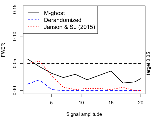
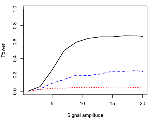
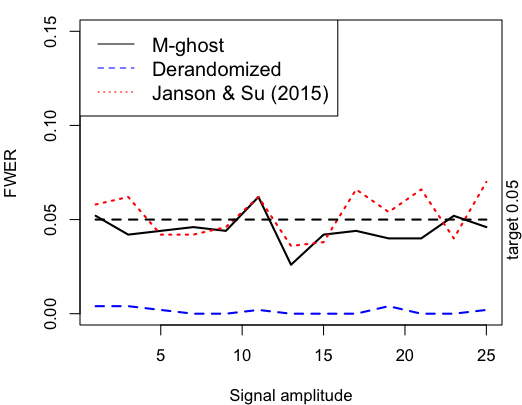
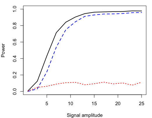
Figure 2: Empirical FWER and power over $500$ simulated datasets of the proposed FWER filter with GhostKnockoff, derandomized knockoffs and the procedure of Janson and Su, (2016) with respect to different signal amplitudes $A$ under compound symmetry (top panel) and AR(1) (bottom panel) correlation structure, sample size $n=500$, dimension $p=100$, correlation strength $\rho=0.5$ and the number of nonnull features $|\mathcal{H}_{1}|=5$.

With the correlation coefficient $\rho=0.5$ and the target FWER level $0.05$, average power of different methods over $500$ datasets under compound symmetry structure and $\text{AR}(1)$ structure is presented in Figure 2. With FWER controlled under the target level, the power of the proposed FWER filter with GhostKnockoff and derandomized knockoffs increase as the signal amplitude $A$ grows under both structures, while the procedure of Janson and Su, (2016) maintains a low power. The reason is that the procedure of Janson and Su, (2016) only makes rejection with probability $2\times 0.05=0.1$ as shown in Section 2.3, making the power bounded by $0.1$. Although the proposed FWER filter with GhostKnockoff dominates derandomized knockoffs in power under both structures, its power can only reach $1$ as $A$ grows under $\text{AR}(1)$ structure and converges to a limit smaller than 1 under the compound symmetry structure. More results under different dimensions and correlation strengths are also provided in Appendix C.1 with similar conclusions.

4.2 Correlation Strength

To further investigate how correlation strength affects the performance of the proposed FWER filter with GhostKnockoff, we generate $500$ datasets for each possible correlation strength $\rho\in\{0,0.1,\ldots,0.9\}$ under both compound symmetry and $\text{AR}(1)$ structure. With a fixed sample size $n=500$, $100$-dimensional features are sampled as i.i.d. observations $\textbf{x}_{1},\ldots,\textbf{x}_{n}\sim\text{N}(0,\mathbf{\Sigma})$ and responses $y_{1},\ldots,y_{n}$ are computed from the linear model (12). With a fixed number of nonzero elements $|\mathcal{H}_{1}|=5$ in the parameter vector $\boldsymbol{\beta}=(\beta_{1},\ldots,\beta_{p})^{\mathsf{T}}$, locations of these nonzero elements are obtained by uniformly sampling of $\{1,\ldots,p\}$ without replacement while their values are i.i.d. uniform variables in $\{A/\sqrt{n},-A/\sqrt{n}\}$. The amplitude $A$ is $6$ and $8$ under compound symmetry and $\text{AR}(1)$ structure respectively to completely show how power varies with respect to correlation strength. To avoid the power loss phenomenon when the SDP construction of $\mathbf{D}$ is used under the compound symmetry structure with $\rho\geq 0.5$ as discovered in Spector and Janson, (2022), we adopt their strategy by multiplying $\mathbf{D}$ with a perturbation factor $\gamma=0.9$.

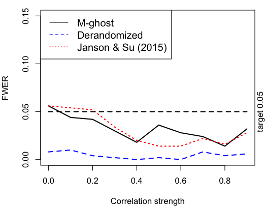
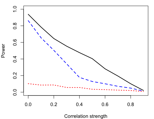
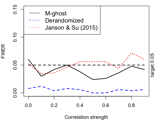
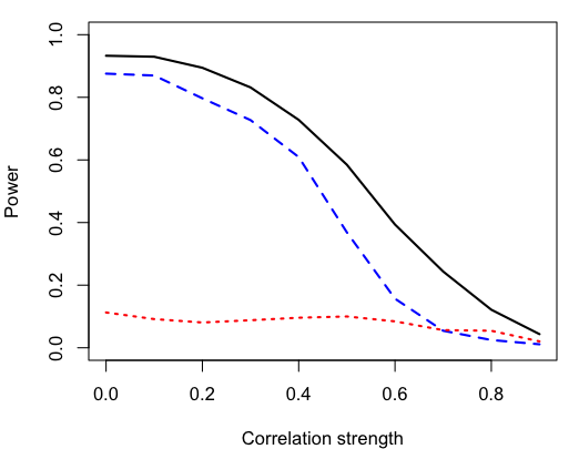
Figure 3: Empirical FWER and power over $500$ simulated datasets of the proposed FWER filter with GhostKnockoff, derandomized knockoffs and the procedure of Janson and Su, (2016) with respect to different correlation strengths $\rho$ under compound symmetry (top panel with $A=6$) and AR(1) (bottom panel with $A=8$) correlation structure, sample size $n=500$, dimension $p=100$ and the number of nonnull features $|\mathcal{H}_{1}|=5$.

Empirical FWER and power of the proposed FWER filter with GhostKnockoff and other existing approaches are visualized in Figure 3. Consistent with our theoretical derivation, our method can control the FWER under the target level $\alpha=0.05$. While the procedure of Janson and Su, (2016) remains powerless, both the proposed FWER filter with GhostKnockoff and knockoffs have a decreasing power as the correlation strength $\rho$ grows. The main reason is that when $\rho$ gets larger, nearby features become more similar, making it more difficult to distinguish true signals. Even though, our method still outperforms derandomized knockoffs, whose power has a sudden drop when $\rho\geq 0.5$ due to the perturbation factor $\gamma$.

4.3 Number of Nonnull Features and Sample Size

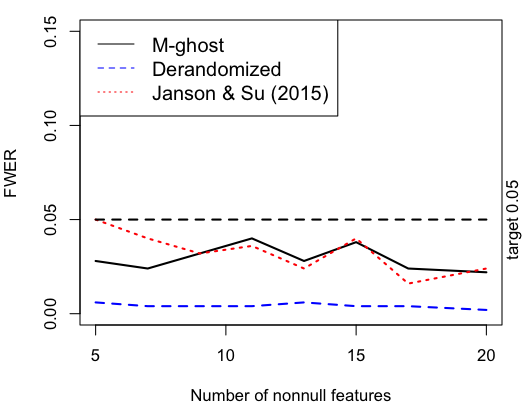
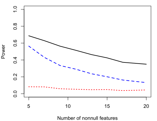
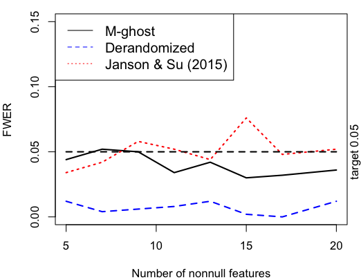
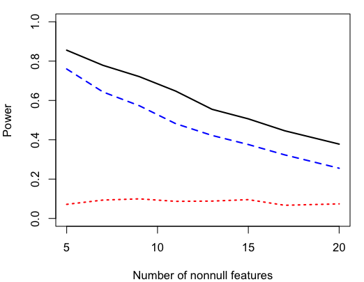
Figure 4: Empirical FWER and power over $500$ simulated datasets of the proposed FWER filter with GhostKnockoff, derandomized knockoffs and the procedure of Janson and Su, (2016) with respect to different numbers of nonnull features $|\mathcal{H}_{1}|$ under compound symmetry (top panel with $A=6$) and AR(1) (bottom panel with $A=8$) correlation structure, sample size $n=500$, dimension $p=200$ and the correlation strength $\rho=0.25$.

To demonstrate the empirical performance of the proposed FWER filter with GhostKnockoff under different number of nonnull features, we generate 500 datasets for each possible number of nonnull features $|\mathcal{H}_{1}|=5,6,\ldots,20$ under both compound symmetry (amplitude $A=6$) and AR(1) (amplitude $A=8$) structures with sample size $n=500$, dimension $p=200$ and correlation strength $\rho=0.25$. Empirical FWER and power of the proposed FWER filter with GhostKnockoff under different $|\mathcal{H}_{1}|$ are visualized in Figures 4, with comparison to derandomized knockoffs and the procedure of Janson and Su, (2016). Similarly, we also simulate 500 datasets for sample sizes $n=100,200,500$ and $1000$ under both compound symmetry (amplitude $A=6$) and AR(1) (amplitude $A=8$) structures with $p=200$, $|\mathcal{H}_{1}|=5$ and $\rho=0.25$. Empirical FWER and power of the proposed FWER filter with GhostKnockoff and existing methods under different sample sizes are shown in Figures 5.

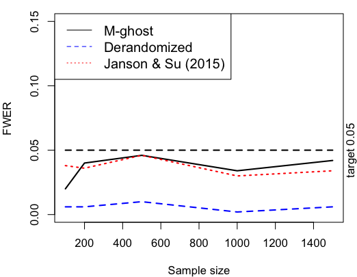
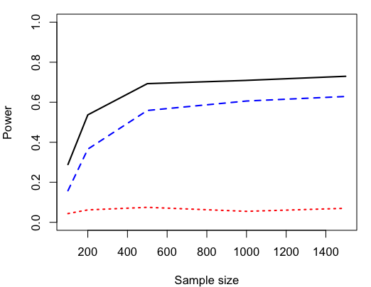
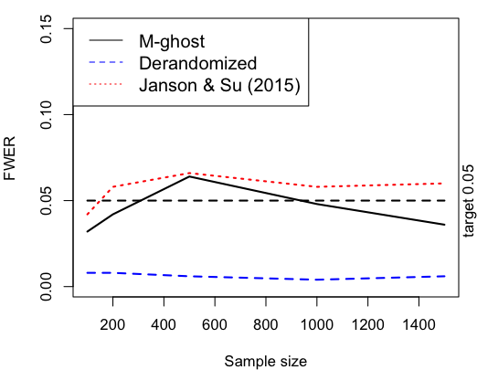
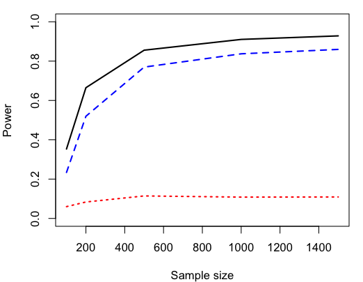
Figure 5: Empirical FWER and power over $500$ simulated datasets of the proposed FWER filter with GhostKnockoff, derandomized knockoffs and the procedure of Janson and Su, (2016) with respect to different sample sizes $n$ under compound symmetry (top panel with $A=6$) and AR(1) (bottom panel with $A=8$) correlation structure, dimension $p=200$, the correlation strength $\rho=0.25$ and numbers of nonnull features $|\mathcal{H}_{1}|=5$.

From Figure 4, it is found that as the number of nonnull features $|\mathcal{H}_{1}|$ grows, the power of both the proposed FWER filter with GhostKnockoff and derandomized knockoffs decreases, suggesting that their ability to detect nonnull features deteriorates under dense but weak signals. As the sample size $n$ increases, the power of both methods grows to $1$ as shown in Figure 5, implying their consistency. In contrast, the procedure of Janson and Su, (2016) keeps a bounded power under $10\%$ throughout all scenarios. More results under different correlation strengths are provided in Appendix C.2 with similar conclusions.

The main reason why the power of the proposed method decreases with respect to $|\mathcal{H}_{1}|$ and increases with respect to $n$ is that the signal-to-noise ratio is of the order $\Omega(\sqrt{n/|\mathcal{H}_{1}|})$. This can be seen in the following toy example. Consider i.i.d. samples $\textbf{x}_{1},\ldots,\textbf{x}_{n}\sim\text{N}(\textbf{0},\textbf{I})$ and responses $y_{1},\ldots,y_{n}$ generated from the linear model (12), where $\beta_{1}=\ldots=\beta_{k}=A/\sqrt{n}$ and $\beta_{k+1}=\cdots=\beta_{p}=0$ for some integer $k$. In other words, we have $|\mathcal{H}_{1}|=k$. By definition (3) of $Z$-scores after standardizing both features and the response, we have $Z_{j}=\sqrt{n}\hat{\rho}_{j}$ where $\hat{\rho}_{j}$ is the empirical correlation of $X_{j}$ and $Y$. By (12), we have $\text{Var}(X_{j})=1$ ($j=1,\ldots,p$), $\text{Cov}(X_{j},Y)=\beta_{j}$ and $\text{Var}(Y)=\sum_{j=1}^{p}\beta_{j}^{2}+1$, leading to true correlations ${\rho}_{j}$ as

$$\rho_{j}=\frac{\text{Cov}(X_{j},Y)}{\sqrt{\text{Var}(X_{j})\text{Var}(Y)}}=\begin{cases}\frac{A/\sqrt{n}}{\sqrt{kA^{2}/n+1}},&j=1,\ldots,k;\\ 0,&\text{otherwise}.\end{cases}$$

By the central limit theorem of correlation coefficient (Lehmann,, 1999) that

$$\sqrt{n}(\hat{\rho}_{j}-\rho_{j})\mathop{\longrightarrow}^{\text{D}}\text{N}(0,(1-\rho_{j}^{2})^{2}),\quad\text{where }\mathop{\longrightarrow}^{\text{D}}\text{ stands for convergence in distribution,}$$

we have that as the amplitude $A$ grows, the expected mean of $Z_{j}$ for nonnull features is $\sqrt{n/k}\{1+o(1)\}$. Since the mean and asymptotic variance of $Z_{j}$ corresponding to null features remain $0$ and $1$, the signal-to-noise ratio is $\Omega(\sqrt{n/k})$. Thus, smaller $|\mathcal{H}_{1}|$ and larger sample size would both lead to larger signal-to-noise ratio and higher power.

5 Real Data Analysis

To investigate the empirical performance of the proposed FWER filter with GhostKnockoff in detecting genetic variants associated with the Alzheimer’s disease (AD), we apply it on the aggregated summary statistics of genetic variants from nine overlapping large-scale array-based genome-wide association studies, and whole-exome/-genome sequencing studies on individuals with European ancestry as summarized in Table 2. Since AD is believed to occur when an abnormal amount of amyloid beta (a type of plasma protein) accumulates in brains (Tackenberg et al.,, 2020), we extract $Z$-scores of $7,963$ variants in protein quantitative trait loci (pQTL) that are reported in Ferkingstad et al., (2021) to have significant association with the level of at least one plasma protein. For comparison, we also apply derandomized knockoffs (Ren et al.,, 2023) on the same datasets.

Table 2: Information of selected large-scale array-based genome-wide association studies, and whole-exome/-genome sequencing studies.

Studies	Sample Size
	AD case samples	Control Sample
The genome-wide survival association study (Huang et al.,, 2017)	14,406	25,849
The genome-wide meta-analysis of clinically diagnosed AD and AD-by-proxy (Jansen et al.,, 2019)	71,880	383,378
The genome-wide meta-analysis of clinically diagnosed AD (Kunkle et al.,, 2019)	21,982	41,944
The genome-wide meta-analysis by Schwartzentruber et al., (2021)	75,024	397,844
In-house genome-wide associations study (Belloy et al., 2022a, )	15,209	14,452
Whole-exome sequencing analyses of data from ADSP by Bis et al., (2020)	5,740	5,096
Whole-exome sequencing analyses of data from ADSP by Le Guen et al., (2021)	6,008	5,119
In-house whole-exome sequencing analysis of ADSP	6,155	5,418
In-house whole-genome sequencing analysis of the 2021 ADSP release (Belloy et al., 2022b, )	3,584	2,949
ADSP: The Alzheimer’s Disease Sequencing Project

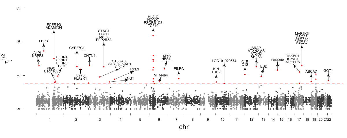
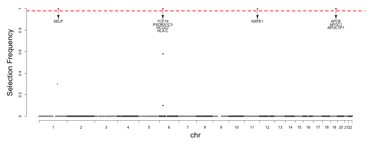
Figure 6: (Top) Manhattan plot of $\sqrt{\tau_{l}}$’s (truncated at 24 for better visualization) from the proposed FWER filter with GhostKnockoff with $M=19$. (Three variant groups are omitted with $\sqrt{\tau_{l}}$’s greatly larger than $24$, including group 19:45416178, group 11:114408449 and group 19:45425178). The selected variant groups under the target FWER level $\alpha=0.05$ are highlighted in red with information of close genes. (Bottom) Manhattan plot of selection frequency from derandomized knockoffs with $M_{deran}=19$. The selected variant groups under the target FWER level $\alpha=0.05$ are highlighted in red with information of close genes.

Corresponding to all $7,963$ variants, we first estimate their covariance matrix $\boldsymbol{\Sigma}$ using genotypes from the UK Biobank data. Although we can apply the proposed FWER filter with GhostKnockoff on $Z$-scores of individual variants, directly doing so is likely to miss most of AD-associated variants. The reason is that a null variant strongly correlated to a nonnull variant is highly possible to have a large $\tau_{j}$ and a nonzero $\kappa_{j}$, making steps 5-8 of Algorithm 1 terminate at a small $T$. To circumvent such an obstacle, we apply the hierarchical clustering algorithm to build variant groups and aggregate effects of variants. Specifically, we use $(1-|\widehat{\text{cor}}(X_{j},X_{l})|)_{7963\times 7963}$ as the input distance matrix of variants, the “single linkage” criterion and the cutoff distance $0.25$, leading to $5,886$ variant groups in total such that pairwise correlations between variants of different groups are within the interval $[-0.75,0.75]$. Based on such a group structure, we aggregate the effect of all variants in the $l$-th group ($l=1,\ldots,5886$) by computing the chi-square test statistic as

$$\chi_{l}=\textbf{Z}^{\mathsf{T}}_{l\text{-th group}}\boldsymbol{\Sigma}^{-1}_{l\text{-th group}}\textbf{Z}_{l\text{-th group}},$$

where $\textbf{Z}_{l\text{-th group}}$ (or $\boldsymbol{\Sigma}_{l\text{-th group}}$) is the $Z$-score vector (or the covariance matrix) corresponding to variants in the $l$-th group. Analogous to $Z_{j}^{2}$ which approximates $n$ times the $R$-squared of the linear model that regresses $Y$ on the $j$-th variant, $\chi_{l}$ approximates $n$ times the $R$-squared of the linear model that regresses $Y$ on variants in the $l$-th group. Under the definition that groups with at least one nonnull variants are nonnull, we apply the proposed FWER filter with GhostKnockoff to estimate nonnull groups as follows.

• Generate knockoff copies of $Z$-scores, $\widetilde{\textbf{Z}}^{1:M}$, via Algorithm 2. Here, $\textbf{D}=\text{diag}(\textbf{S}_{1},\ldots,\textbf{S}_{5886})$ is a block diagonal matrix with respect to variant groups obtained by solving the optimization problem,

  $$\min\sum_{l=1}^{5886}p_{l}^{-2}\|\textbf{S}_{l}-\boldsymbol{\Sigma}_{l}\|_{1,1}\quad\quad\text{ s.t. }\begin{cases}\frac{M+1}{M}\mathbf{\Sigma-D}\succeq 0,\\ \textbf{S}_{l}=\boldsymbol{\Lambda}_{l}+\sum_{k=1}^{p_{l}}\delta_{lk}\textbf{v}_{lk}\textbf{v}_{lk}^{\mathsf{T}},\quad 1\leq l\leq 5886,\end{cases}$$

  where $\|\cdot\|_{1,1}$ is the $L_{1,1}$ matrix norm and for $l=1,\ldots,5886$,

  • $p_{l}$ and $\boldsymbol{\Sigma}_{l}$ are the size and the correlation matrix of the $l$-th variant group respectively,

  • $\boldsymbol{\Lambda}_{l}\succeq 0$ is a diagonal matrix,

  • $\textbf{v}_{l1},\ldots,\textbf{v}_{lp_{l}}$ are eigenvectors of $\boldsymbol{\Sigma}_{l}$,

  • $\delta_{l1},\ldots,\delta_{lp_{l}}$ are nonnegative;

• Compute knockoff copies of chi-square test statistics $\{\chi_{l}^{m}|l=1,\ldots,5886;m=1,\ldots,M\}$ via

  $$\chi^{m}_{l}=(\widetilde{\textbf{Z}}^{m}_{l\text{-th group}})^{\mathsf{T}}\boldsymbol{\Sigma}^{-1}_{l\text{-th group}}\widetilde{\textbf{Z}}^{m}_{l\text{-th group}};$$

• Compute the knockoff statistic of the $l$-th variant group as

  $$\kappa_{l}=\underset{0\leq m\leq M}{\arg\max}\text{ }(\chi_{l}^{m})^{2},\quad\tau_{l}=(\chi_{l}^{\kappa_{l}})^{2}-\underset{m\neq\kappa_{l}}{\operatorname{median}}(\chi_{l}^{m})^{2},\quad(l=1,\ldots,5886).$$ (15)

• Apply Algorithm 1 on $\{(\kappa_{l},\tau_{l})|l=1,\ldots,5886\}$ to obtain the rejection set of variant groups.

Analogously, derandomized knockoffs (Ren et al.,, 2023) are also implemented on SDP-constructed group knockoff copies with $M_{deran}=50$ and $\eta=0.99$ using codes of Ren et al., (2023).

With the number of knockoff copies $M=19$ and the target FWER level $\alpha=0.05$, the proposed FWER filter with GhostKnockoff manages to reject 42 variant groups as shown in top panel of Figure 6 and Table 3. Similar to the literature, several groups (groups 19:45416178, 19:45425178, 19:45505803 and 19:45322744) are rejected in the APOE/APOC region with the strongest association to AD. In addition, the proposed FWER filter with GhostKnockoff can detect nonnull groups within 1Mb distance to genes “ADAMTS4” (groups 1:161152778 and 1:169529132), “FAM20B” (group 1:172412995), “BIN1” (group 2:127882182), “HLA-DQA1” (groups 6:31195793, 6:32202086, 6:31229796, 6:31900657 and 6:32623367) and “ABCA7” (group 19:1051137), which are also reported in the work of He et al., (2022). In contrast, only 5 groups are rejected by derandomized knockoffs ($M_{deran}=50$ and $\eta=0.98$). As shown in bottom panel of Figure 6, with only 8 variant groups have nonzero selection frequency and 5 variants have selection frequency $1$, derandomized knockoffs can not detect any variant group near genes “BIN1” and “HLA-DQA1”, which are of strong significance in He et al., (2022). This is mainly due to the bounded power of the procedure of Janson and Su, (2016) underlying the derandomized procedure as shown in Section 4, suggesting the advantage of the proposed FWER filter with GhostKnockoff.

Table 3: Details of variant groups rejected by the proposed FWER filter with GhostKnockoff ($M=19$) under the target FWER level $\alpha=0.05$. Groups that are also rejected by derandomized knockoffs ($M_{deran}=50$ and $\eta=0.98$) are highlighted in bold. Here, groups are named in terms of ”a:b” if its leading variant is at position b of chromosome a.

Group	Chromosome	Positions of variants	Close genes
19:45416178	19	45411941, 45413576, 45415713, 45416178, 45416741, 45422160	APOE, APOC1
11:114408449	11	114405806, 114407012, 114407750, 114408449	NXPE1
19:45425178	19	45412079, 45425178, 45426792	APOE, APOC1P1
6:31195793	6	31121945, 31142265, 31149520, 31154633, 31195793, 31195996, 31197074, 31200816, 31206868, 31234693	TCF19, PSORS1C3, HCG27, HLA-C
1:66092570	1	66092570, 66109445	LEPR
6:32202086	6	31914935, 32109165, 32202086, 32278635, 32416366, 32523008, 32560266	CFB, PRRT1, TSBP1-AS1, TSBP1, HLA-DRA, HLA-DRB6, HLA-DRB1
1:161152778	1	161152778, 161186313	ADAMTS4, FCER1G
6:31229796	6	31229796, 31239114	HLA-C
6:31900657	6	31887259, 31891491, 31893257, 31900657, 31903804, 31909340, 31919830, 32156895	C2, C2-AS1, CFB, NELFE, GPSM3
17:67276383	17	67081278, 67134806, 67136325, 67249711, 67276383, 67424508	ABCA6, ABCA10, ABCA5, MAP2K6
3:2713965	3	2713965, 2716366	CNTN4
1:21817085	1	21775943, 21806447, 21817085, 21820042, 21821897, 21822699	NBPF3, ALPL
2:127882182	2	127882182	CYP27C1
12:111932800	12	111865049, 111884608, 111904371, 111907431, 111932800, 112007756, 112059557	SH2B3, ATXN2, ATXN2-AS, BRAP
3:135998453	3	135798658, 135800409, 135804550, 135833005, 135846911, 135925191, 135926622, 135932359, 135950921, 135965888, 135998453, 136003159, 136020541, 136027145, 136095035, 136162621	PPP2R3A, MSL2, PCCB, STAG1
6:32623367	6	32590735, 32591310, 32615457, 32623367, 32626451, 32626537, 32632770	HLA-DQA1, HLA-DQB1, HLA-DQB1-AS1
6:135427817	6	135402339, 135418632, 135418916, 135421176, 135422296, 135423209, 135426573, 135427159, 135427817, 135428537, 135432552, 135435501	HBS1L, MYB
2:160821211	2	160718332, 160734382, 160760972, 160778946, 160799625, 160821211	LY75, PLA2R1
6:29821340	6	29821340, 29822432, 29908415, 29921619, 29923136	HCP5B, HLA-A
14:106387308	14	106358616, 106363591, 106369865, 106371016, 106383775, 106384722, 106387308, 106392575	FAM30A
17:45766771	17	45571676, 45735706, 45737275, 45763073, 45766771	NPEPPS, KPNB1, TBKBP1
19:45505803	19	45445517, 45505803, 45507542, 45522289	APOC4-APOC2, RELB
12:7178019	12	7170336, 7171338, 7171507, 7172665, 7175872, 7176204, 7176978, 7178019, 7179822, 7181948	C1S, C1R
1:196822368	1	196679682, 196681001, 196698945, 196721931, 196725939, 196815711, 196819479, 196821120, 196821380, 196822368, 196825287	CFH, CFHR3, CFHR1, CFHR4
13:47351403	13	47351403, 47368296	ESD
3:98406933	3	98359663, 98383562, 98406794, 98406933, 98416900, 98417481, 98428155, 98429219, 98431986, 98432559, 98443648, 98453951	CPOX, ST3GAL6-AS1, ST3GAL6
7:99971834	7	99971834	PILRA
6:32441696	6	32441696, 32584926	HLA-DRA, HLA-DQA1
19:45322744	19	45322744	BCAM
4:39446337	4	39446337, 39447604	RPL9
22:24997309	22	24997309, 25002323	GGT1
6:90935383	6	90935383, 90960875	MIR4464
1:172412995	1	172400009, 172400860, 172412995, 172421744, 172425529	C1orf105, PIGC
19:1051137	19	1051137	ABCA7
6:31878108	6	31878108, 31878581	C2
3:186449122	3	186445052, 186449122, 186450863	KNG1
10:7769806	10	7749598, 7756187, 7764233, 7769806, 7770716, 7772035, 7774358, 7774728	ITIH2, KIN
1:169529132	1	169529132, 169549811, 169562904	SELP
2:234665983	2	234587848, 234664586, 234665782, 234665983, 234668570, 234673309	UGT1A7, LOC100286922, UGT1A1
17:44200015	17	43849415, 43897026, 44200015	CRHR1, MAPT-AS1, KANSL1-AS1
6:41129207	6	41129207	TREM2
10:82267945	10	82267945, 82284512	LOC101929574

6 Discussions

In this article, we develop a novel filter to simultaneously test multiple hypotheses of conditional independence with FWER control using GhostKnockoff. Under the Gaussian assumption of features, we follow the procedure of He et al., (2022) to directly generate $M$ knockoff copies of summary statistics without using any individual data and propose a FWER filter with GhostKnockoff to estimate the set of nonnull features. By selecting features whose knockoff statistics $\kappa_{j}$’s are zero and $\tau_{j}$’s are larger than the maximum value of $\tau_{j}$ among features with nonzero $\kappa_{j}$’s, our method manages to circumvent the power bound in Janson and Su, (2016) when the target FWER level is smaller than $1/2$. Furthermore, an elaborated algorithm is proposed to significantly reduce the computational cost of knockoff copies generation from $O(M^{3}p^{3})$ to $O(p^{3})$ without any loss in FWER control and power. Through extensive simulations on synthetic and real datasets, the proposed FWER filter with GhostKnockoff exhibits valid control on FWER and superior power in detecting nonnull features over existing methods, including derandomized knockoffs and the procedure of Janson and Su, (2016).

There are several directions available for further studies. As the proposed FWER filter with GhostKnockoff is an one-shot procedure, its inference has inevitably large variation due to the uncertainty in sampling knockoff copies $\widetilde{\textbf{Z}}^{1:M}$. Thus, it is possible to incorporate the proposed method in the derandomized procedure of Ren et al., (2023). By substituting the procedure of Janson and Su, (2016) to be repeated in derandomized knockoffs, we can simultaneously achieve inference stability, high power and computation efficiency. For example, using the proposed FWER filter with GhostKnockoff with $M=5$ and $v=1$ as the based procedure, the derandomized procedure (Ren et al.,, 2023) can control FWER under $\alpha=0.05$ with smaller $M_{deran}=10$ and $\eta=0.89$ compared to the setting in Section 4 ($M_{deran}=50$ and $\eta=0.99$). As shown in simulations, both the proposed FWER filter with GhostKnockoff and derandomized knockoffs are bounded in power when features are correlated. Such a phenomenon is mainly due to the mismatching between $Z$-scores, which generally depict marginal correlations, and the conditional independence (1) we target to test. Therefore, it is worth investigating how to develop feature importance scores to directly depict conditional correlations with only summary statistics. One possible solution is to use $\mathbf{\widetilde{Z}}^{0},\dots\mathbf{\widetilde{Z}}^{M}$ and matrices $\boldsymbol{\Sigma}$ and D to obtain the approximate lasso estimator of the linear model $Y=\boldsymbol{\beta}^{\mathsf{T}}\mathbf{X}+\sum_{m=1}^{M}(\widetilde{\boldsymbol{\beta}}^{m})^{\mathsf{T}}\widetilde{\mathbf{X}}^{m}+\epsilon$ as feature importance scores. By doing so, magnitudes of feature importance scores corresponding to nonnull features would increase as the signal amplitude $A$ grows and keep unchanged as the number of nonnull features $|\mathcal{H}_{1}|$ increases, getting rid of the power bound phenomenon shown in Section 4. In addition, when the number of features $p$ is large as in genome-wide analyses, it is highly possible to have some null features with nonzero $\kappa_{j}$’s and large $\tau_{j}$’s, leading to early stop in nonnull features selection and power loss. Thus, it is of great interest to incorporate some power boosting strategies to the proposed FWER filter with GhostKnockoff, including the feature screening technique (Barber and Candès,, 2019) and incorporating side information (Ren and Candès,, 2023).

Appendix A Proof of Lemma 1

Proof of Lemma 1.

Let $\widetilde{Z}_{j}^{m,\star}=\widetilde{Z}_{j}^{\sigma_{j}(m)}$ for $j=1,\ldots,p$ and $m=0,\ldots,M$, we have for any $\boldsymbol{\sigma}=\{\sigma_{1},\ldots,\sigma_{p}\}$ where $\sigma_{j}$ is any permutation on $\{0,1,\ldots,M\}$ if $H_{j}$ is true and is the identity permutation if $H_{j}$ is false ($j=1,\ldots,p$),

$$\begin{cases}\kappa_{j}^{\star}=\underset{0\leq m\leq M}{\arg\max}\text{ }(\widetilde{Z}_{j}^{m,\star})^{2}=\sigma_{j}^{-1}(\kappa_{j}),&j\in\mathcal{H}_{0},\\ \kappa_{j}^{\star}=\underset{0\leq m\leq M}{\arg\max}\text{ }(\widetilde{Z}_{j}^{m,\star})^{2}=\kappa_{j},&j\in\mathcal{H}_{1},\\ \tau^{\star}_{j}=(\widetilde{Z}_{j}^{\kappa_{j}})^{2}-\underset{m\neq\kappa_{j}}{\operatorname{median}}(\widetilde{Z}_{j}^{m,\star})^{2}=\tau_{j},&j=1,\ldots,p.\\ \end{cases}$$ (16)

Since $Z$-scores $\mathbf{\widetilde{Z}}^{0},\dots\mathbf{\widetilde{Z}}^{M}$ possess the extended exchangeability property (8) with respect to $\{H_{j}:j=1,\ldots,p\}$, we have

$$\bigg{[}\{\kappa_{j}|j\in\mathcal{H}_{0}\}\bigg{|}\{\kappa_{j}|j\notin\mathcal{H}_{0}\},\{\tau_{j}|j=1,\ldots,p\}\bigg{]}{\buildrel d\over{=}}\bigg{[}\{\sigma_{j}^{-1}(\kappa_{j})|j\in\mathcal{H}_{0}\}\bigg{|}\{\kappa_{j}|j\notin\mathcal{H}_{0}\},\{\tau_{j}|j=1,\ldots,p\}\bigg{]}.$$

Because $\sigma_{j}$ can be any permutation for all $j\in\mathcal{H}_{0}$, $\sigma_{j}^{-1}$ can also be any permutation. Thus, $\{\kappa_{j}|j\in\mathcal{H}_{0}\}$ are independent uniform random variables on $\{0,1,\ldots,M\}$ conditional on $\{\kappa_{j}|j\notin\mathcal{H}_{0}\}$ and $\{\tau_{j}|j=1,\ldots,p\}$. ∎

Appendix B Proof of extended exchangeability property of $Z$-scores $\mathbf{\widetilde{Z}}^{0},\mathbf{\widetilde{Z}}^{1},\dots\mathbf{\widetilde{Z}}^{M}$

As shown in He et al., (2022), when the Gaussian model $\textbf{X}\sim\text{N}(\mathbf{0},\boldsymbol{\Sigma})$ is assumed to generate $M$-knockoffs $(\mathbf{\widetilde{X}}^{1},\dots\mathbf{\widetilde{X}}^{M})$, knockoff copies of $Z$-score $\mathbf{\widetilde{Z}}^{1},\dots\mathbf{\widetilde{Z}}^{M}$ defined by (4) satisfy (5). Thus, we have $\widetilde{Z}^{m}_{j}$ is a function of $\widetilde{\mathbb{X}}^{m}_{j}=\{\widetilde{x}^{m}_{ij}:i=1,\ldots,n\}$ and $\mathbb{Y}=\{y_{i}:i=1,\ldots,n\}$

$$\widetilde{Z}^{m}_{j}=\nu(\widetilde{\mathbb{X}}^{m}_{j},\mathbb{Y})$$

for any $m=0,\ldots,M$ and $j=1,\ldots,p$ under the convention $\mathbf{\widetilde{x}}_{i}^{0}=\textbf{x}_{i}$ ($i=1,\ldots,n$).

For any $\boldsymbol{\sigma}=\{\sigma_{1},\ldots,\sigma_{p}\}$ where

$$\begin{cases}\sigma_{j}\text{ is any permutation on }\{0,1,\ldots,M\},&\text{if }H_{j}\text{ is true (or }j\in\mathcal{H}_{0}\text{),}\\ \sigma_{j}\text{ is the identity permutation, }&\text{if }H_{j}\text{ is false (or }j\in\mathcal{H}_{1}\text{),}\\ \end{cases}$$ (17)

we have

$$\mathbf{\widetilde{Z}}^{0:M}_{swap(\boldsymbol{\sigma})} =(\widetilde{Z}^{\sigma_{1}(0)}_{1},\ldots,\widetilde{Z}^{\sigma_{p}(0)}_{p},\ldots,\widetilde{Z}^{\sigma_{1}(M)}_{1},\ldots,\widetilde{Z}^{\sigma_{p}(M)}_{p})^{\mathsf{T}}$$ (18)

$$=(\nu(\widetilde{\mathbb{X}}^{\sigma_{1}(0)}_{1},\mathbb{Y}),\ldots,\nu(\widetilde{\mathbb{X}}^{\sigma_{p}(0)}_{p},\mathbb{Y}),\ldots,\nu(\widetilde{\mathbb{X}}^{\sigma_{1}(M)}_{1},\mathbb{Y}),\ldots,\nu(\widetilde{\mathbb{X}}^{\sigma_{p}(M)}_{p},\mathbb{Y}))^{\mathsf{T}}.$$

By the conditional independence property of multiple knockoffs (Gimenez and Zou,, 2019) that

$$(\mathbf{\widetilde{X}}^{1},\dots\mathbf{\widetilde{X}}^{M})\perp Y|\mathbf{\widetilde{X}}^{0}$$

and hypotheses (1), we have $(\mathbf{\widetilde{X}}^{0}_{\mathcal{H}_{0}},\mathbf{\widetilde{X}}^{1},\dots\mathbf{\widetilde{X}}^{M})\perp Y|\mathbf{\widetilde{X}}^{0}_{\mathcal{H}_{1}}$ where $\mathbf{\widetilde{X}}^{0}_{\mathcal{H}_{0}}$ (or $\mathbf{\widetilde{X}}^{0}_{\mathcal{H}_{1}}$) is the subvector of $\mathbf{\widetilde{X}}^{0}$ corresponding to $\mathcal{H}_{0}$ (or $\mathcal{H}_{1}$). Thus, the joint distribution of $(\mathbf{\widetilde{X}}^{0},\mathbf{\widetilde{X}}^{1},\dots\mathbf{\widetilde{X}}^{M},Y)$ satisfies

$$F(\mathbf{\widetilde{X}}^{0:M},Y) =F(\mathbf{\widetilde{X}}^{0}_{\mathcal{H}_{1}})F(\mathbf{\widetilde{X}}^{0}_{\mathcal{H}_{0}},\mathbf{\widetilde{X}}^{1},\dots\mathbf{\widetilde{X}}^{M}|\mathbf{\widetilde{X}}^{0}_{\mathcal{H}_{1}})F(Y|\mathbf{\widetilde{X}}^{0}_{\mathcal{H}_{1}})$$

$$=F(\mathbf{\widetilde{X}}^{0:M})F(Y|\mathbf{\widetilde{X}}^{0}_{\mathcal{H}_{1}})$$

By the exchangeability property of multiple knockoffs (Gimenez and Zou,, 2019) that

$$\mathbf{\widetilde{X}}^{0:M}_{swap(\boldsymbol{\sigma})}=(\widetilde{X}^{\sigma_{1}(0)}_{1},\ldots,\widetilde{X}^{\sigma_{p}(0)}_{p},\ldots,\widetilde{X}^{\sigma_{1}(M)}_{1},\ldots,\widetilde{X}^{\sigma_{p}(M)}_{p})^{\mathsf{T}}\,{\buildrel d\over{=}}\,\mathbf{\widetilde{X}}^{0:M},$$

we have for any $\boldsymbol{\sigma}$ satisfies (17),

$$F(\mathbf{\widetilde{X}}_{swap(\boldsymbol{\sigma})}^{0:M},Y) =F(\mathbf{\widetilde{X}}_{swap(\boldsymbol{\sigma})}^{0:M})F(Y|\mathbf{\widetilde{X}}^{0}_{\mathcal{H}_{1}})$$ (19)

$$=F(\mathbf{\widetilde{X}}^{0:M})F(Y|\mathbf{\widetilde{X}}^{0}_{\mathcal{H}_{1}})$$

$$=F(\mathbf{\widetilde{X}}^{0:M},Y).$$

In conclusion, we have for any $\boldsymbol{\sigma}$ satisfies (17), by (18) and (19),

$$F(\mathbf{\widetilde{Z}}_{swap(\boldsymbol{\sigma})}^{0:M}){\buildrel d\over{=}}F(\mathbf{\widetilde{Z}}^{0:M}),$$

and thus $\mathbf{\widetilde{Z}}^{0:M}$ possess extended exchangeability property (8).

Appendix C Additional Simulation Results

C.1 Correlation Structure

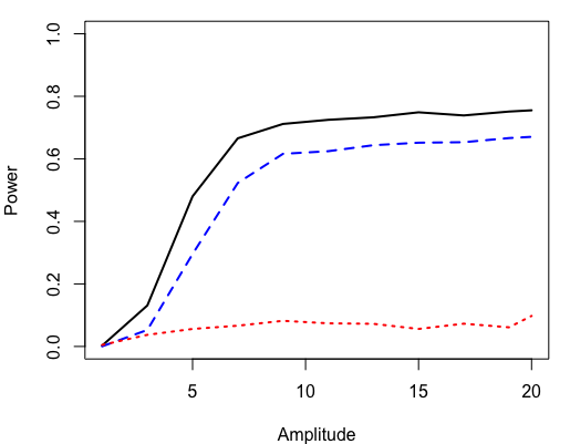
(a) Correlation strength $\rho=0.25$.

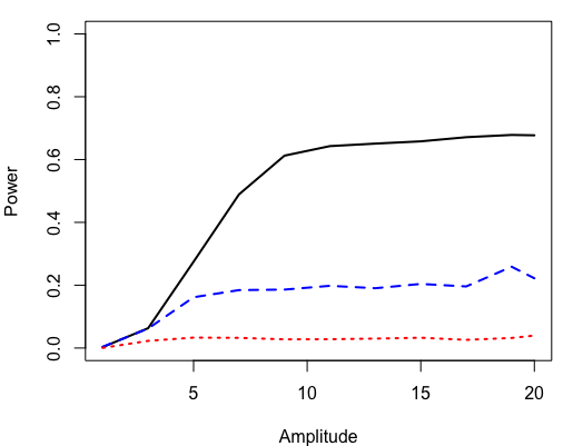
(b) Correlation strength $\rho=0.5$.

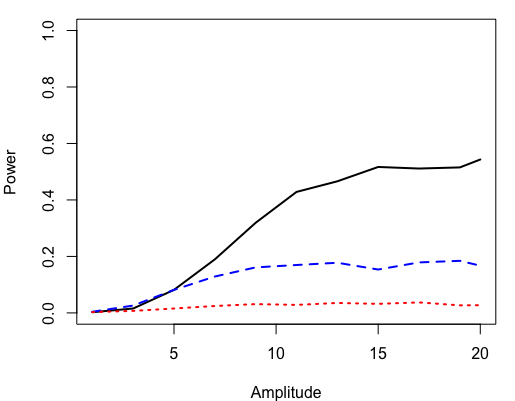
(c) Correlation strength $\rho=0.75$.

Figure 7: Empirical power over $500$ simulated datasets of the proposed FWER filter with GhostKnockoff (black solid line), derandomized knockoffs (blue dashed line) and the procedure of Janson and Su, (2016) (red dotted line) with respect to different signal amplitudes $A$ and different correlation strengths under compound symmetry correlation structure, sample size $n=500$, dimension $p=100$, number of nonnull features $|\mathcal{H}_{1}|=5$, the target FWER level $\alpha=0.05$.

(a) Dimension $p=100$.

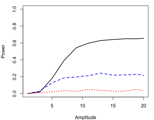
(b) Dimension $p=500$.

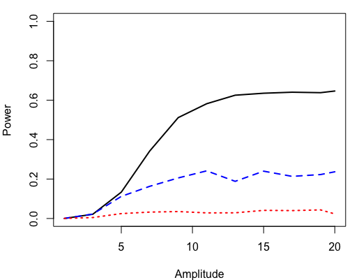
(c) Dimension $p=1000$.

Figure 8: Empirical power over $500$ simulated datasets of the proposed FWER filter with GhostKnockoff (black solid line), derandomized knockoffs (blue dashed line) and the procedure of Janson and Su, (2016) (red dotted line) with respect to different signal amplitudes $A$ and different dimensions under compound symmetry correlation structure, sample size $n=500$, correlation strength $\rho=0.5$, number of nonnull features $|\mathcal{H}_{1}|=5$, the target FWER level $\alpha=0.05$.

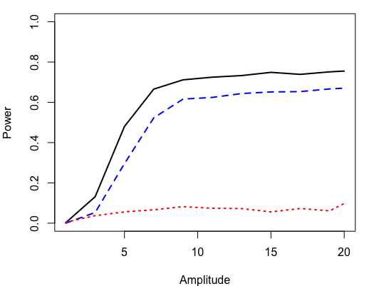
(a) Correlation strength $\rho=0.25$.

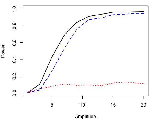
(b) Correlation strength $\rho=0.5$.

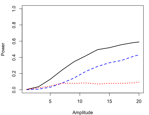
(c) Correlation strength $\rho=0.75$.

Figure 9: Empirical power over $500$ simulated datasets of the proposed FWER filter with GhostKnockoff (black solid line), derandomized knockoffs (blue dashed line) and the procedure of Janson and Su, (2016) (red dotted line) with respect to different signal amplitudes $A$ and different correlation strengths under compound correlation structure, sample size $n=500$, dimension $p=100$, number of nonnull features $|\mathcal{H}_{1}|=5$, the target FWER level $\alpha=0.05$.

(a) Dimension $p=100$.

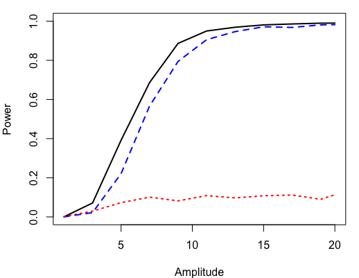
(b) Dimension $p=500$.

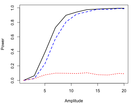
(c) Dimension $p=1000$.

Figure 10: Empirical power over $500$ simulated datasets of the proposed FWER filter with GhostKnockoff (black solid line), derandomized knockoffs (blue dashed line) and the procedure of Janson and Su, (2016) (red dotted line) with respect to different signal amplitudes $A$ and different dimensions under AR(1) correlation structure, sample size $n=500$, correlation strength $\rho=0.5$, number of nonnull features $|\mathcal{H}_{1}|=5$, the target FWER level $\alpha=0.05$.

C.2 Number of Nonnull Features and Sample Size

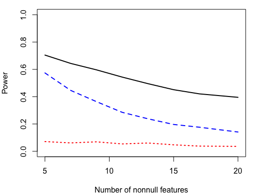
(a) Correlation strength $\rho=0.25$.

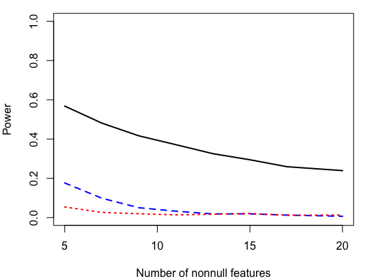
(b) Correlation strength $\rho=0.5$.

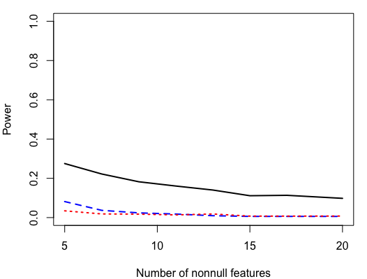
(c) Correlation strength $\rho=0.75$.

Figure 11: Empirical power over $500$ simulated datasets of the proposed FWER filter with GhostKnockoff (black solid line), derandomized knockoffs (blue dashed line) and the procedure of Janson and Su, (2016) (red dotted line) with respect to different numbers of nonnull features $|\mathcal{H}_{1}|$ and different correlation strengths under compound symmetry correlation structure, sample size $n=500$, dimension $p=100$, amplitude strength $A=6$, the target FWER level $\alpha=0.05$.

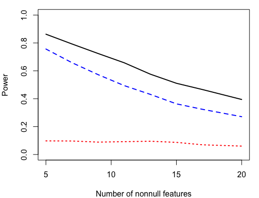
(a) Correlation strength $\rho=0.25$.

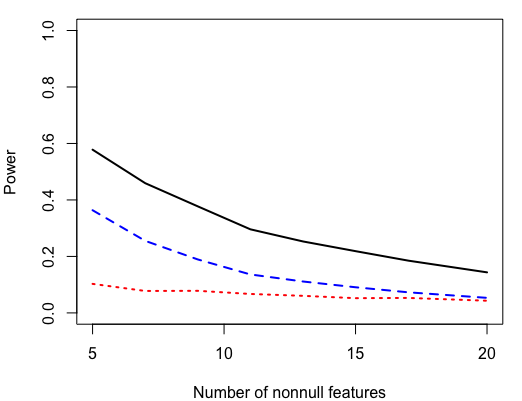
(b) Correlation strength $\rho=0.5$.

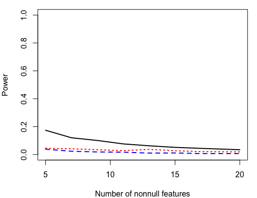
(c) Correlation strength $\rho=0.75$.

Figure 12: Empirical power over $500$ simulated datasets of the proposed FWER filter with GhostKnockoff (black solid line), derandomized knockoffs (blue dashed line) and the procedure of Janson and Su, (2016) (red dotted line) with respect to different numbers of nonnull features $|\mathcal{H}_{1}|$ and different correlation strengths under AR(1) correlation structure, sample size $n=500$, dimension $p=100$, amplitude strength $A=8$, the target FWER level $\alpha=0.05$.

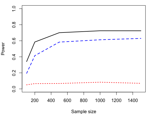
(a) Correlation strength $\rho=0.25$.

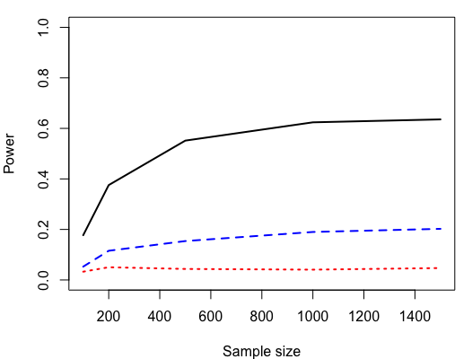
(b) Correlation strength $\rho=0.5$.

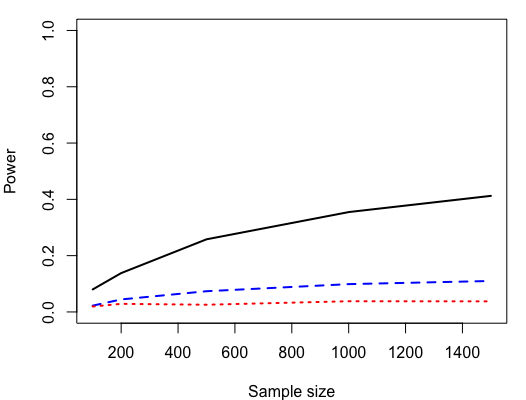
(c) Correlation strength $\rho=0.75$.

Figure 13: Empirical power over $500$ simulated datasets of the proposed FWER filter with GhostKnockoff (black solid line), derandomized knockoffs (blue dashed line) and the procedure of Janson and Su, (2016) (red dotted line) with respect to different sample sizes $n$ and different correlation strengths under compound symmetry correlation structure, dimension $p=100$, number of nonnull features $|\mathcal{H}_{1}|=5$, amplitude strength $A=6$, the target FWER level $\alpha=0.05$.

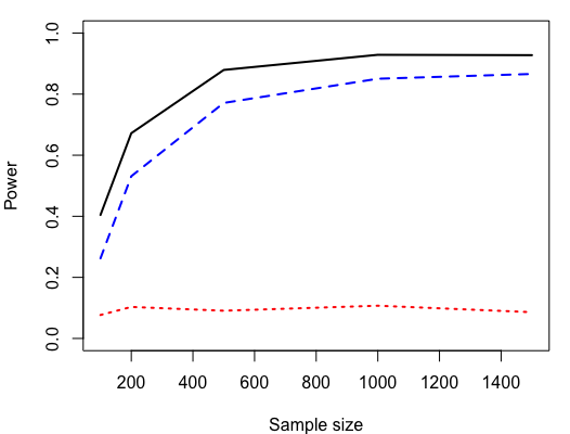
(a) Correlation strength $\rho=0.25$.

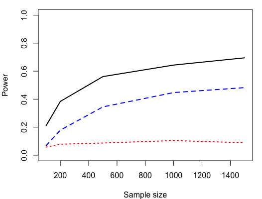
(b) Correlation strength $\rho=0.5$.

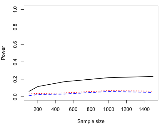
(c) Correlation strength $\rho=0.75$.

Figure 14: Empirical power over $500$ simulated datasets of the proposed FWER filter with GhostKnockoff (black solid line), derandomized knockoffs (blue dashed line) and the procedure of Janson and Su, (2016) (red dotted line) with respect to different sample sizes $n$ and different correlation strengths under AR(1) correlation structure, dimension $p=100$, number of nonnull features $|\mathcal{H}_{1}|=5$, amplitude strength $A=8$, the target FWER level $\alpha=0.05$.

References

- Barber and Candès, (2015) Barber, R. F. and Candès, E. J. (2015). Controlling the false discovery rate via knockoffs. The Annals of Statistics, 43(5):2055–2085.
- Barber and Candès, (2019) Barber, R. F. and Candès, E. J. (2019). A knockoff filter for high-dimensional selective inference. The Annals of Statistics, 47(5):2504–2537.
- (3) Belloy, M. E., Eger, S. J., Le Guen, Y., Damotte, V., Ahmad, S., Ikram, M. A., Ramirez, A., Tsolaki, A. C., Rossi, G., Jansen, I. E., de Rojas, I., Parveen, K., Sleegers, K., Ingelsson, M., Hiltunen, M., Amin, N., Andreassen, O., Sánchez-Juan, P., Kehoe, P., Amouyel, P., Sims, R., Frikke-Schmidt, R., van der Flier, W. M., Lambert, J.-C., for the European Alzheimer & Dementia BioBank (EADB), He, Z., Han, S. S., Napolioni, V., and Greicius, M. D. (2022a). Challenges at the APOE locus: a robust quality control approach for accurate APOE genotyping. Alzheimer’s Research & Therapy, 14(1):22.
- (4) Belloy, M. E., Le Guen, Y., Eger, S. J., Napolioni, V., Greicius, M. D., and He, Z. (2022b). A Fast and Robust Strategy to Remove Variant-Level Artifacts in Alzheimer Disease Sequencing Project Data. Neurology Genetics, 8(5):e200012.
- Benjamini and Hochberg, (1995) Benjamini, Y. and Hochberg, Y. (1995). Controlling the False Discovery Rate: A Practical and Powerful Approach to Multiple Testing. Journal of the Royal Statistical Society: Series B (Methodological), 57:289–300.
- Benjamini and Yekutieli, (2001) Benjamini, Y. and Yekutieli, D. (2001). The control of the false discovery rate in multiple testing under dependency. The Annals of Statistics, 29(4):1165–1188.
- Bis et al., (2020) Bis, J. C., Jian, X., Kunkle, B. W., Chen, Y., Hamilton-Nelson, K. L., Bush, W. S., Salerno, W. J., Lancour, D., Ma, Y., Renton, A. E., Marcora, E., Farrell, J. J., Zhao, Y., Qu, L., Ahmad, S., Amin, N., Amouyel, P., Beecham, G. W., Below, J. E., Campion, D., Cantwell, L., Charbonnier, C., Chung, J., Crane, P. K., Cruchaga, C., Cupples, L. A., Dartigues, J.-F., Debette, S., Deleuze, J.-F., Fulton, L., Gabriel, S. B., Genin, E., Gibbs, R. A., Goate, A., Grenier-Boley, B., Gupta, N., Haines, J. L., Havulinna, A. S., Helisalmi, S., Hiltunen, M., Howrigan, D. P., Ikram, M. A., Kaprio, J., Konrad, J., Kuzma, A., Lander, E. S., Lathrop, M., Lehtimäki, T., Lin, H., Mattila, K., Mayeux, R., Muzny, D. M., Nasser, W., Neale, B., Nho, K., Nicolas, G., Patel, D., Pericak-Vance, M. A., Perola, M., Psaty, B. M., Quenez, O., Rajabli, F., Redon, R., Reitz, C., Remes, A. M., Salomaa, V., Sarnowski, C., Schmidt, H., Schmidt, M., Schmidt, R., Soininen, H., Thornton, T. A., Tosto, G., Tzourio, C., van der Lee, S. J., van Duijn, C. M., Valladares, O., Vardarajan, B., Wang, L.-S., Wang, W., Wijsman, E., Wilson, R. K., Witten, D., Worley, K. C., Zhang, X., Bellenguez, C., Lambert, J.-C., Kurki, M. I., Palotie, A., Daly, M., Boerwinkle, E., Lunetta, K. L., Destefano, A. L., Dupuis, J., Martin, E. R., Schellenberg, G. D., Seshadri, S., Naj, A. C., Fornage, M., and Farrer, L. A. (2020). Whole exome sequencing study identifies novel rare and common Alzheimer’s-Associated variants involved in immune response and transcriptional regulation. Molecular Psychiatry, 25(8):1859–1875.
- Candes et al., (2018) Candes, E., Fan, Y., Janson, L., and Lv, J. (2018). Panning for Gold: ‘Model-X’ Knockoffs for High Dimensional Controlled Variable Selection. Journal of the Royal Statistical Society: Series B (Statistical Methodology), 80(3):551–577.
- Daudin, (1980) Daudin, J. (1980). Partial association measures and an application to qualitative regression. Biometrika, 67(3):581–590.
- Dawid, (1979) Dawid, A. P. (1979). Conditional Independence in Statistical Theory. Journal of the Royal Statistical Society: Series B (Methodological), 41:1–15.
- Doran et al., (2014) Doran, G., Muandet, K., Zhang, K., and Schölkopf, B. (2014). A permutation-based kernel conditional independence test. In Proceedings of the Thirtieth Conference on Uncertainty in Artificial Intelligence, pages 132–141.
- Dunn, (1961) Dunn, O. J. (1961). Multiple Comparisons among Means. Journal of the American Statistical Association, 56(293):52–64.
- Fan et al., (2020) Fan, Y., Lv, J., Sharifvaghefi, M., and Uematsu, Y. (2020). IPAD: Stable Interpretable Forecasting with Knockoffs Inference. Journal of the American Statistical Association, 115(532):1822–1834.
- Ferkingstad et al., (2021) Ferkingstad, E., Sulem, P., Atlason, B. A., Sveinbjornsson, G., Magnusson, M. I., Styrmisdottir, E. L., Gunnarsdottir, K., Helgason, A., Oddsson, A., Halldorsson, B. V., Jensson, B. O., Zink, F., Halldorsson, G. H., Masson, G., Arnadottir, G. A., Katrinardottir, H., Juliusson, K., Magnusson, M. K., Magnusson, O. T., Fridriksdottir, R., Saevarsdottir, S., Gudjonsson, S. A., Stacey, S. N., Rognvaldsson, S., Eiriksdottir, T., Olafsdottir, T. A., Steinthorsdottir, V., Tragante, V., Ulfarsson, M. O., Stefansson, H., Jonsdottir, I., Holm, H., Rafnar, T., Melsted, P., Saemundsdottir, J., Norddahl, G. L., Lund, S. H., Gudbjartsson, D. F., Thorsteinsdottir, U., and Stefansson, K. (2021). Large-scale integration of the plasma proteome with genetics and disease. Nature Genetics, 53:1712–1721.
- Gimenez and Zou, (2019) Gimenez, J. R. and Zou, J. (2019). Improving the Stability of the Knockoff Procedure: Multiple Simultaneous Knockoffs and Entropy Maximization. In Proceedings of the Twenty-Second International Conference on Artificial Intelligence and Statistics, volume 89, pages 2184–2192. PMLR.
- He et al., (2022) He, Z., Liu, L., Belloy, M. E., Le Guen, Y., Sossin, A., Liu, X., Qi, X., Ma, S., Gyawali, P. K., Wyss-Coray, T., Tang, H., Sabatti, C., Candès, E., Greicius, M. D., and Ionita-Laza, I. (2022). GhostKnockoff inference empowers identification of putative causal variants in genome-wide association studies. Nature Communications, 13:7209.
- He et al., (2021) He, Z., Liu, L., Wang, C., Le Guen, Y., Lee, J., Gogarten, S., Lu, F., Montgomery, S., Tang, H., Silverman, E. K., Cho, M. H., Greicius, M., and Ionita-Laza, I. (2021). Identification of putative causal loci in whole-genome sequencing data via knockoff statistics. Nature Communications, 12:3152.
- Hochberg, (1988) Hochberg, Y. (1988). A sharper Bonferroni procedure for multiple tests of significance. Biometrika, 75(4):800–802.
- Holm, (1979) Holm, S. (1979). A Simple Sequentially Rejective Multiple Test Procedure. Scandinavian Journal of Statistics, 6(2):65–70.
- Huang et al., (2017) Huang, K.-L., Marcora, E., Pimenova, A. A., Narzo, A. F. D., Kapoor, M., Jin, S. C., Harari, O., Bertelsen, S., Fairfax, B. P., Czajkowski, J., Chouraki, V., Grenier-Boley, B., Bellenguez, C., Deming, Y., McKenzie, A., Raj, T., Renton, A. E., Budde, J., Smith, A., Fitzpatrick, A., Bis, J. C., DeStefano, A., Adams, H. H. H., Ikram, M. A., van der Lee, S., Del-Aguila, J. L., Fernandez, M. V., Ibañez, L., Sims, R., Escott-Price, V., Mayeux, R., Haines, J. L., Farrer, L. A., Pericak-Vance, M. A., Lambert, J. C., van Duijn, C., Launer, L., Seshadri, S., Williams, J., Amouyel, P., Schellenberg, G. D., Zhang, B., Borecki, I., Kauwe, J. S. K., Cruchaga, C., Hao, K., and Goate, A. M. (2017). A common haplotype lowers PU.1 expression in myeloid cells and delays onset of Alzheimer’s disease. Nature Neuroscience, 20:1052–1061.
- Jansen et al., (2019) Jansen, I. E., Savage, J. E., Watanabe, K., Bryois, J., Williams, D. M., Steinberg, S., Sealock, J., Karlsson, I. K., Hägg, S., Athanasiu, L., Voyle, N., Proitsi, P., Witoelar, A., Stringer, S., Aarsland, D., Almdahl, I. S., Andersen, F., Bergh, S., Bettella, F., Bjornsson, S., Brækhus, A., Bråthen, G., de Leeuw, C., Desikan, R. S., Djurovic, S., Dumitrescu, L., Fladby, T., Hohman, T. J., Jonsson, P. V., Kiddle, S. J., Rongve, A., Saltvedt, I., Sando, S. B., Selbæk, G., Shoai, M., Skene, N. G., Snaedal, J., Stordal, E., Ulstein, I. D., Wang, Y., White, L. R., Hardy, J., Hjerling-Leffler, J., Sullivan, P. F., van der Flier, W. M., Dobson, R., Davis, L. K., Stefansson, H., Stefansson, K., Pedersen, N. L., Ripke, S., Andreassen, O. A., and Posthuma, D. (2019). Genome-wide meta-analysis identifies new loci and functional pathways influencing Alzheimer’s disease risk. Nature Genetics, 51:404–413.
- Janson and Su, (2016) Janson, L. and Su, W. (2016). Familywise error rate control via knockoffs. Electronic Journal of Statistics, 10(1):960–975.
- Katsevich and Sabatti, (2019) Katsevich, E. and Sabatti, C. (2019). Multilayer knockoff filter: Controlled variable selection at multiple resolutions. The Annals of Applied Statistics, 13(1):1–33.
- Khera and Kathiresan, (2017) Khera, A. V. and Kathiresan, S. (2017). Genetics of coronary artery disease: discovery, biology and clinical translation. Nature Reviews Genetics, 18:331–344.
- Kunkle et al., (2019) Kunkle, B. W., , Grenier-Boley, B., Sims, R., Bis, J. C., Damotte, V., Naj, A. C., Boland, A., Vronskaya, M., van der Lee, S. J., Amlie-Wolf, A., Bellenguez, C., Frizatti, A., Chouraki, V., Martin, E. R., Sleegers, K., Badarinarayan, N., Jakobsdottir, J., Hamilton-Nelson, K. L., Moreno-Grau, S., Olaso, R., Raybould, R., Chen, Y., Kuzma, A. B., Hiltunen, M., Morgan, T., Ahmad, S., Vardarajan, B. N., Epelbaum, J., Hoffmann, P., Boada, M., Beecham, G. W., Garnier, J.-G., Harold, D., Fitzpatrick, A. L., Valladares, O., Moutet, M.-L., Gerrish, A., Smith, A. V., Qu, L., Bacq, D., Denning, N., Jian, X., Zhao, Y., Zompo, M. D., Fox, N. C., Choi, S.-H., Mateo, I., Hughes, J. T., Adams, H. H., Malamon, J., Sanchez-Garcia, F., Patel, Y., Brody, J. A., Dombroski, B. A., Naranjo, M. C. D., Daniilidou, M., Eiriksdottir, G., Mukherjee, S., Wallon, D., Uphill, J., Aspelund, T., Cantwell, L. B., Garzia, F., Galimberti, D., Hofer, E., Butkiewicz, M., Fin, B., Scarpini, E., Sarnowski, C., Bush, W. S., Meslage, S., Kornhuber, J., White, C. C., Song, Y., Barber, R. C., Engelborghs, S., Sordon, S., Voijnovic, D., Adams, P. M., Vandenberghe, R., Mayhaus, M., Cupples, L. A., Albert, M. S., Deyn, P. P. D., Gu, W., Himali, J. J., Beekly, D., Squassina, A., Hartmann, A. M., Orellana, A., Blacker, D., Rodriguez-Rodriguez, E., Lovestone, S., Garcia, M. E., Doody, R. S., Munoz-Fernadez, C., Sussams, R., Lin, H., Fairchild, T. J., Benito, Y. A., Holmes, C., Karamujić-Čomić, H., Frosch, M. P., Thonberg, H., Maier, W., Roshchupkin, G., Ghetti, B., Giedraitis, V., Kawalia, A., Li, S., Huebinger, R. M., Kilander, L., Moebus, S., Hernández, I., Kamboh, M. I., Brundin, R., Turton, J., Yang, Q., Katz, M. J., Concari, L., Lord, J., Beiser, A. S., Keene, C. D., Helisalmi, S., Kloszewska, I., Kukull, W. A., Koivisto, A. M., Lynch, A., Tarraga, L., Larson, E. B., Haapasalo, A., Lawlor, B., Mosley, T. H., Lipton, R. B., Solfrizzi, V., Gill, M., Longstreth, W. T., Montine, T. J., Frisardi, V., Diez-Fairen, M., Rivadeneira, F., Petersen, R. C., Deramecourt, V., Alvarez, I., Salani, F., Ciaramella, A., Boerwinkle, E., Reiman, E. M., Fievet, N., Rotter, J. I., Reisch, J. S., Hanon, O., Cupidi, C., Uitterlinden, A. G. A., Royall, D. R., Dufouil, C., Maletta, R. G., de Rojas, I., Sano, M., Brice, A., Cecchetti, R., George-Hyslop, P. S., Ritchie, K., Tsolaki, M., Tsuang, D. W., Dubois, B., Craig, D., Wu, C.-K., Soininen, H., Avramidou, D., Albin, R. L., Fratiglioni, L., Germanou, A., Apostolova, L. G., Keller, L., Koutroumani, M., Arnold, S. E., Panza, F., Gkatzima, O., Asthana, S., Hannequin, D., Whitehead, P., Atwood, C. S., Caffarra, P., Hampel, H., Quintela, I., Carracedo, Á., Lannfelt, L., Rubinsztein, D. C., Barnes, L. L., Pasquier, F., Frölich, L., Barral, S., McGuinness, B., Beach, T. G., Johnston, J. A., Becker, J. T., Passmore, P., Bigio, E. H., Schott, J. M., Bird, T. D., Warren, J. D., Boeve, B. F., Lupton, M. K., Bowen, J. D., Proitsi, P., Boxer, A., Powell, J. F., Burke, J. R., Kauwe, J. S. K., Burns, J. M., Mancuso, M., Buxbaum, J. D., Bonuccelli, U., Cairns, N. J., McQuillin, A., Cao, C., Livingston, G., Carlson, C. S., Bass, N. J., Carlsson, C. M., Hardy, J., Carney, R. M., Bras, J., Carrasquillo, M. M., Guerreiro, R., Allen, M., Chui, H. C., Fisher, E., Masullo, C., Crocco, E. A., DeCarli, C., Bisceglio, G., Dick, M., Ma, L., Duara, R., Graff-Radford, N. R., Evans, D. A., Hodges, A., Faber, K. M., Scherer, M., Fallon, K. B., Riemenschneider, M., Fardo, D. W., Heun, R., Farlow, M. R., Kölsch, H., Ferris, S., Leber, M., Foroud, T. M., Heuser, I., Galasko, D. R., Giegling, I., Gearing, M., Hüll, M., Geschwind, D. H., Gilbert, J. R., Morris, J., Green, R. C., Mayo, K., Growdon, J. H., Feulner, T., Hamilton, R. L., Harrell, L. E., Drichel, D., Honig, L. S., Cushion, T. D., Huentelman, M. J., Hollingworth, P., Hulette, C. M., Hyman, B. T., Marshall, R., Jarvik, G. P., Meggy, A., Abner, E., Menzies, G. E., Jin, L.-W., Leonenko, G., Real, L. M., Jun, G. R., Baldwin, C. T., Grozeva, D., Karydas, A., Russo, G., Kaye, J. A., Kim, R., Jessen, F., Kowall, N. W., Vellas, B., Kramer, J. H., Vardy, E., LaFerla, F. M., Jöckel, K.-H., Lah, J. J., Dichgans, M., Leverenz, J. B., Mann, D., Levey, A. I., Pickering-Brown, S., Lieberman, A. P., Klopp, N., Lunetta, K. L., Wichmann, H.-E., Lyketsos, C. G., Morgan, K., Marson, D. C., Brown, K., Martiniuk, F., Medway, C., Mash, D. C., Nöthen, M. M., Masliah, E., Hooper, N. M., McCormick, W. C., Daniele, A., McCurry, S. M., Bayer, A., McDavid, A. N., Gallacher, J., McKee, A. C., van den Bussche, H., Mesulam, M., Brayne, C., Miller, B. L., Riedel-Heller, S., Miller, C. A., Miller, J. W., Al-Chalabi, A., Morris, J. C., Shaw, C. E., Myers, A. J., Wiltfang, J., O’Bryant, S., Olichney, J. M., Alvarez, V., Parisi, J. E., Singleton, A. B., Paulson, H. L., Collinge, J., Perry, W. R., Mead, S., Peskind, E., Cribbs, D. H., Rossor, M., Pierce, A., Ryan, N. S., Poon, W. W., Nacmias, B., Potter, H., Sorbi, S., Quinn, J. F., Sacchinelli, E., Raj, A., Spalletta, G., Raskind, M., Caltagirone, C., Bossù, P., Orfei, M. D., Reisberg, B., Clarke, R., Reitz, C., Smith, A. D., Ringman, J. M., Warden, D., Roberson, E. D., Wilcock, G., Rogaeva, E., Bruni, A. C., Rosen, H. J., Gallo, M., Rosenberg, R. N., Ben-Shlomo, Y., Sager, M. A., Mecocci, P., Saykin, A. J., Pastor, P., Cuccaro, M. L., Vance, J. M., Schneider, J. A., Schneider, L. S., Slifer, S., Seeley, W. W., Smith, A. G., Sonnen, J. A., Spina, S., Stern, R. A., Swerdlow, R. H., Tang, M., Tanzi, R. E., Trojanowski, J. Q., Troncoso, J. C., Deerlin, V. M. V., Eldik, L. J. V., Vinters, H. V., Vonsattel, J. P., Weintraub, S., Welsh-Bohmer, K. A., Wilhelmsen, K. C., Williamson, J., Wingo, T. S., Woltjer, R. L., Wright, C. B., Yu, C.-E., Yu, L., Saba, Y., Pilotto, A., Bullido, M. J., Peters, O., Crane, P. K., Bennett, D., Bosco, P., Coto, E., Boccardi, V., Jager, P. L. D., Lleo, A., Warner, N., Lopez, O. L., Ingelsson, M., Deloukas, P., Cruchaga, C., Graff, C., Gwilliam, R., Fornage, M., Goate, A. M., Sanchez-Juan, P., Kehoe, P. G., Amin, N., Ertekin-Taner, N., Berr, C., Debette, S., Love, S., Launer, L. J., Younkin, S. G., Dartigues, J.-F., Corcoran, C., Ikram, M. A., Dickson, D. W., Nicolas, G., Campion, D., Tschanz, J., Schmidt, H., Hakonarson, H., Clarimon, J., Munger, R., Schmidt, R., Farrer, L. A., Broeckhoven, C. V., O’Donovan, M. C., DeStefano, A. L., Jones, L., Haines, J. L., Deleuze, J.-F., Owen, M. J., Gudnason, V., Mayeux, R., Escott-Price, V., Psaty, B. M., Ramirez, A., Wang, L.-S., Ruiz, A., van Duijn, C. M., Holmans, P. A., Seshadri, S., Williams, J., Amouyel, P., Schellenberg, G. D., Lambert, J.-C., and Pericak-Vance, M. A. (2019). Genetic meta-analysis of diagnosed Alzheimer’s disease identifies new risk loci and implicates A, tau, immunity and lipid processing. Nature Genetics, 51(3):414–430.
- Le Guen et al., (2021) Le Guen, Y., Belloy, M. E., Napolioni, V., Eger, S. J., Kennedy, G., Tao, R., He, Z., and Greicius, M. D. (2021). A novel age-informed approach for genetic association analysis in Alzheimer’s disease. Alzheimer’s Research & Therapy, 13:72.
- Lehmann, (1999) Lehmann, E. L. (1999). Elements of Large-Sample Theory. Springer New York, NY.
- Luo et al., (2022) Luo, Y., Fithian, W., and Lei, L. (2022). Improving knockoffs with conditional calibration. arXiv preprint arXiv:2208.09542.
- Patel et al., (2015) Patel, J., Shah, S., Thakkar, P., and Kotecha, K. (2015). Predicting stock and stock price index movement using Trend Deterministic Data Preparation and machine learning techniques. Expert Systems with Applications, 42(1):259–268.
- Peters et al., (2014) Peters, J., Mooij, J. M., Janzing, D., and Schölkopf, B. (2014). Causal Discovery with Continuous Additive Noise Models. Journal of Machine Learning Research, 15(58):2009–2053.
- Ren and Candès, (2023) Ren, Z. and Candès, E. (2023). Knockoffs with side information. The Annals of Applied Statistics, 17(2):1152–1174.
- Ren et al., (2023) Ren, Z., Wei, Y., and Candès, E. (2023). Derandomizing Knockoffs. Journal of the American Statistical Association, 118(542):948–958.
- Schwartzentruber et al., (2021) Schwartzentruber, J., Cooper, S., Liu, J. Z., Barrio-Hernandez, I., Bello, E., Kumasaka, N., Young, A. M. H., Franklin, R. J. M., Johnson, T., Estrada, K., Gaffney, D. J., Beltrao, P., and Bassett, A. (2021). Genome-wide meta-analysis, fine-mapping and integrative prioritization implicate new Alzheimer’s disease risk genes. Nature Genetics, 53:392–402.
- Sen et al., (2017) Sen, R., Suresh, A. T., Shanmugam, K., Dimakis, A. G., and Shakkottai, S. (2017). Model-powered Conditional Independence test. In Proceedings of the 31st International Conference on Neural Information Processing Systems, page 2955–2965.
- Šidák, (1967) Šidák, Z. (1967). Rectangular Confidence Regions for the Means of Multivariate Normal Distributions. Journal of the American Statistical Association, 62(318):626–633.
- Spector and Janson, (2022) Spector, A. and Janson, L. (2022). Powerful knockoffs via minimizing reconstructability. The Annals of Statistics, 50(1):252 – 276.
- Storey, (2003) Storey, J. D. (2003). The positive false discovery rate: a Bayesian interpretation and the -value. The Annals of Statistics, 31(6):2013–2035.
- Tackenberg et al., (2020) Tackenberg, C., Kulic, L., and Nitsch, R. M. (2020). Familial Alzheimer’s disease mutations at position 22 of the amyloid -peptide sequence differentially affect synaptic loss, tau phosphorylation and neuronal cell death in an ex vivo system. PLoS ONE, 15(9):e0239584.
- Zhu et al., (2018) Zhu, Z., Zheng, Z., Zhang, F., Wu, Y., Trzaskowski, M., Maier, R., Robinson, M. R., McGrath, J. J., Visscher, P. M., Wray, N. R., and Yang, J. (2018). Causal associations between risk factors and common diseases inferred from GWAS summary data. Nature communications, 9:224.