Study of residual artificial neural network for particle identification in the CEPC high-granularity calorimeter prototype

Abstract

Particle Identification (PID) plays a central role in associating the energy depositions in calorimeter cells with the type of primary particle in a particle flow oriented detector system. In this paper, we propose novel PID methods based on the Residual Network (ResNet) architecture which enable the training of very deep networks, bypass the need to reconstruct feature variables, and ensure the generalization ability among various geometries of detectors, to classify electromagnetic showers and hadronic showers. Using Geant4 simulation samples with energy ranging from 5 GeV to 120 GeV, the efficacy of Residual Connections is validated and the performance of our model is compared with Boosted Decision Trees (BDT) and other pioneering Artificial Neural Networks (ANN) approaches. In shower classification, we observe an improvement in background rejection over a wide range of high signal efficiency ($>95\%$). These findings highlight the prospects of ANN with Residual Blocks for imaging detectors in the PID task of particle physics experiments.

1 Introduction

The Circular Electron Positron Collider (CEPC), dedicated to precisely measuring the properties of the Higgs boson, incorporates the Particle Flow Algorithm (PFA) [1] in the detector system’s baseline design. The fundamental concept behind the PFA is to utilize the most suitable detector subsystem for accurately determining the energy/momentum of individual particles within a jet. To achieve this objective, PFA-oriented calorimeters require high granularity. In the context of a growing volume of inputs, the development of Particle Identification (PID) methods customized for high-granularity calorimeters holds significance.

High-granularity calorimeters capture the intricate spatial development of showers in unprecedented detail, providing valuable information for PID. Patterns of energy depositions observed in the 3D array of “cells” substantially reflect the characteristics of the type of the primary particle. Typical spatial configurations of shower types are illustrated in figure 1. The electron leads to an electromagnetic shower, and the pion causes a hadronic shower. Distinguishing between electromagnetic and hadronic showers is crucial for gaining insights into the underlying physics processes, while some hadronic showers may contain electromagnetic components, making it difficult to establish clear-cut criteria for classification.

In one way, the MultiVariate Analysis (TMVA) technique [2] reconstructs shower topology feature variables from such 3D images. For instance, in CALICE SDHCAL PID [3], six shower topology variables were reconstructed to build a TMVA Boosted Decision Trees (BDT) classifier [4, 5, 6] for separating electron events from hadron events. The disadvantage of BDT is that it heavily depends on the quality and relevance of the reconstructed feature variables. When compressing massive raw data into several feature variables, systematically finding a set of effective variables that are not highly correlated is challenging, and some hidden features might be missed  [7].

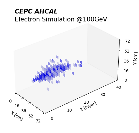
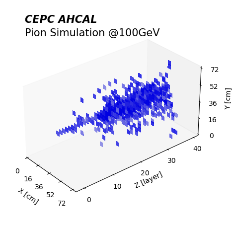
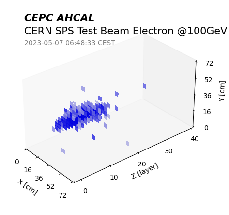
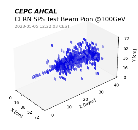
Figure 1: The CEPC Analogue Hadronic Calorimeter (AHCAL) prototype is employed to display different shower types. In the first row, the electron event (a), and the pion event (b) are simulated. In the second row, the electron event (c), and the pion event (d) are selected from the CEPC AHCAL test beam Run files. Their primary energy is 100 GeV.

In another way, Artificial Neural Networks (ANN) have great potential to be applied to high-granularity calorimeter PID [8, 9], offering the advantage of making full use of raw high-dimensional input data, (e.g. spatial distributions of energy depositions). There are two specialized types of ANN, Convolutional Neural Networks (CNN) designed for processing structured grid-like data, such as images, and Graph Neural Networks (GNN) tailored for processing graph-structured data. Recently, ANN has been utilized in various experiments, including the NOvA experiment for neutrino identification [10], the Belle II experiment for the detection of low-momentum muons and pions [11], and the CMS experiment for the identification of hadronic tau lepton decays [12], etc. In common, these methods share a shallow architecture combining 2D convolutional (Conv) layers for feature extraction and fully connected (FC) layers for classification as illustrated in figure 2. Although they have already achieved great success, a specific study of the state-of-the-art deeper architectures such as ResNet[13] and AlexNet[14] on PID has not been conducted. Furthermore, the potential applications of these methods may be limited to detectors with regular geometry, facilitating the preprocessing of data into images. Therefore, there is growing interest in Graph Neural Network (GNN) models, which offer greater flexibility in handling data from detectors with irregular geometries. In this domain, pioneering models such as DGCNN[15] and GravNet[16, 17] have been developed for either classification or clustering.

Figure 2: The 2D convolutional layers are coupled with fully connected layers. The former is for feature extraction while the latter is for classification.

In this paper, we propose novel PID methods based on the ResNet architecture[13], a much deeper architecture with millions of trainable parameters tailored for high-granularity calorimeters. The efficacy of introducing Residual Connections is studied and the final performance is compared with the benchmark BDT[18], LeNet[19], and AlexNet[14] methods. Furthermore, to ensure the generality, an updated model adaptable to any irregular detector geometry, called the Dynamic Graph Residual Networks (DGRes), allowing our ResNet-based model to be applied beyond detectors with regular structures, has been proposed and compared with other GNN models, DGCNN[15] and GravNet[16, 17]. The paper is structured as follows: Section 2 introduces detector geometry and Monte Carlo simulation samples which are used to study the performance of various classifiers, Section 3 briefly illustrates PID based on BDT and provides insights on shower topology; Section 4 demonstrates the algorithm, the performance, and the complexity of our models; Section 5 concludes this research.

2 Detector geometry and Monte Carlo samples

The detector used in this study is the CEPC Analogue Hadronic Calorimeter (AHCAL) prototype featured in high granularity [20, 21, 22]. As illustrated in figure 3, it comprises $40$ sampling layers with steel cassettes and absorbers. In a steel cassette, there are scintillator tiles of size $4\times 4\times 0.3\ \mathrm{cm^{3}}$ coupled with a silicon photomultiplier (SiPM), which are arranged in an $18\times 18$ array. The total number of channels is $12960$. The thickness of steel is $2\ \text{cm/layer}$.

In this context, 960,000 simulation shower samples of single-primary-particle events, perpendicularly entering the AHCAL, are prepared. These samples are represented by 3D images ($18\times 18\times 40$ pixels). To be more specific, the Geant4 11.1.1 Toolkit [23] with the $\mathrm{QGSP\_BERT}$ [24] physics list was employed to conduct a comprehensive investigation into the response of pions and electrons within calorimeters, aiming to examine the behavior of these particles under similar conditions as the experimental setup. In figure 1, we can find that the shower topology of MC samples is close to the shower topology of test beam data, from the perspective of the human eyes. At present, test beam data are still under calibration and check. Therefore, we only employ MC samples in the following sections. It is still sufficient to effectively compare all PID methods since the same MC samples are employed. As listed in table 1, a wide energy range of 5 GeV–120 GeV has been explored, with a uniform mixture of electron and pion events.

Figure 3: The schematic sandwich structure of AHCAL prototype (a). The array of $4\times 4\times 0.3\ \mathrm{cm^{3}}$ scintillator tiles on a PCB (b). One sampling layer contains three PCBs.

Table 1: The composition of MC samples.

Energy point

5 GeV

10 GeV

30 GeV

50 GeV

60 GeV

80 GeV

100 GeV

120 GeV

$\#$

Source

$\#$

Source

$\#$

Source

$\#$

Source

$\#$

Source

$\#$

Source

$\#$

Source

$\#$

Source

Electron

60k

MC

60k

MC

60k

MC

60k

MC

60k

MC

60k

MC

60k

MC

60k

MC

Pion

60k

MC

60k

MC

60k

MC

60k

MC

60k

MC

60k

MC

60k

MC

60k

MC

In order to counteract the risk of overfitting, these samples are subjected to a randomized split into three distinct sets: the training set, validation set, and the test set in a ratio of 2:1:7. The training set and the validation set are used for building the related BDT and ANN classifiers, while the performance of the constructed BDT and ANN classifiers is evaluated using the test set. Each individual sample undergoes the transformation into input compatible with both BDT and ANN methodologies, ensuring a comprehensive and consistent approach to our analysis.

3 PID based on BDT

We apply Extreme Gradient Boosting (XGBoost), which is known for its high performance[18]. In the AHCAL, a conventional right-handed coordinate system is utilized, with its 40 layers arranged perpendicular to the incoming beams. The origin of this coordinate system is established at the center of the first layer. The transverse plane, referred to as the $x$–$y$ plane, runs parallel to the AHCAL layers. The $z$-axis is aligned with the direction of the incoming beam. 12 commonly utilized shower topology variables are reconstructed from the spatial distribution of energy depositions in AHCAL:

• Shower Density: The average number of neighboring hits around one hit, including the hit itself, in a $3\times 3$ cell area in a given event is calculated. The distributions of this quantity, referred to as the shower density, are shown in figure 4. As expected, electromagnetic showers exhibit a more compact distribution compared to hadronic showers.

• Shower Start: The first layer of the first three consecutive layers with at least 5 hits. For events without showers, the shower start layer is set to 42. Electrons start showering virtually in the first 7 layers as illustrated in figure 4.

• Shower End: After the shower starts, the first layer of two consecutive layers with no more than 2 hits. If no shower is formed, it is set to 42. It is illustrated in figure 4 that electromagnetic showers almost end in the first half of the AHCAL.

• Shower Length: The distance between the start of the shower and the layer where the maximum Root Mean Square (RMS) of hit transverse coordinates concerning the $z$-axis occurs. In figure 4, it can be observed that some pions exhibit a longer shower length.

• The total number of hits (Hits Number): In a given event, it represents the total number of hits (figure 4). It can effectively separate electromagnetic showers and hadronic showers.

• Shower Radius: The RMS of the distance with respect to the $z$-axis of AHCAL. Figure 4 illustrates that electrons and pions exhibit distinct values in this variable.

• Fractal dimension (FD): Fractal dimension only depends on the calorimeter observables [25]. By grouping blocks of $\alpha\times\alpha$ cells, where $\alpha$ defines the scale at which the shower is analyzed, $\mathrm{N}_{\alpha}$, as the number of hits at scale $\alpha$, could be calculated. Then, varying a series of $\alpha$ larger than $\beta$, $\mathrm{FD}_{\beta}$ could be derived based on equation 3.1. As shown in figures 4 and 4, pions and electrons exhibit distinct values.

  $$\mathrm{FD}_{\beta}=\left\langle{\frac{\mathrm{log(R_{\alpha,\beta})}}{\mathrm{log(\alpha)}}}\right\rangle+1,\ \mathrm{where}\ \mathrm{R}_{\alpha,\beta}=\mathrm{N}_{\beta}/\mathrm{N}_{\alpha}$$ (3.1)

• The number of layers with hits (Fired Layers): It is defined as the number of layers with at least one hit. In figure 4, we can find that this variable helps to discriminate electron events from pion events.

• Shower layers: The number of layers in which the RMS of positions in the $x$–$y$ plane exceeds $4$ cm in both the $x$ and $y$ directions. Figure 4 illustrates that electrons and pions exhibit distinct values in this variable.

• Ratio of shower layers over fired layers (Shower Layer Ratio): This variable has differences between electrons and pions, as depicted in figure 4.

• Z Depth: The RMS of the $z$-axis coordinates. There is a clear difference between electron events and pion events in this variable, as shown in figure 4.

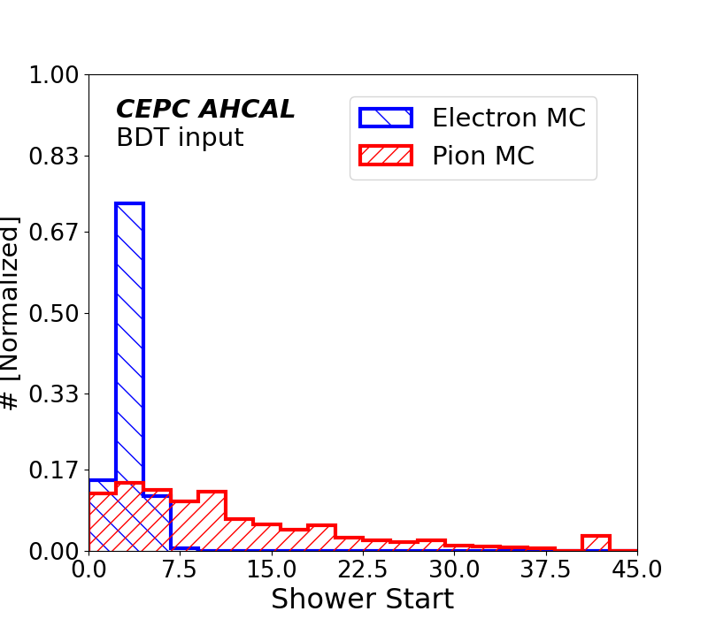
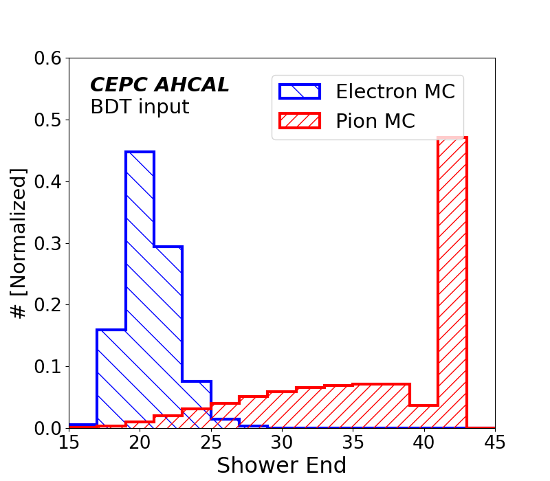
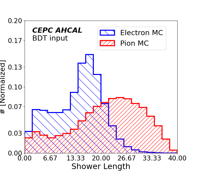
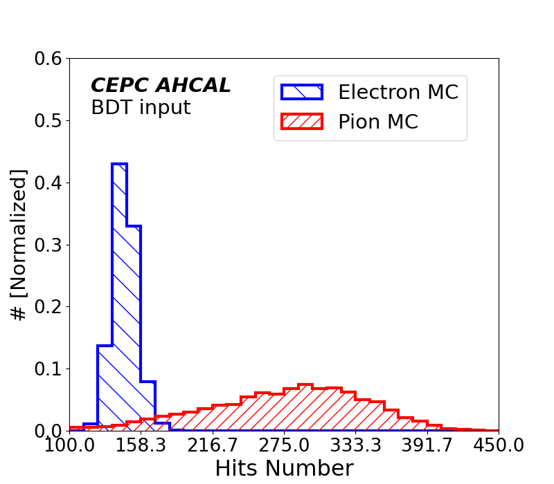
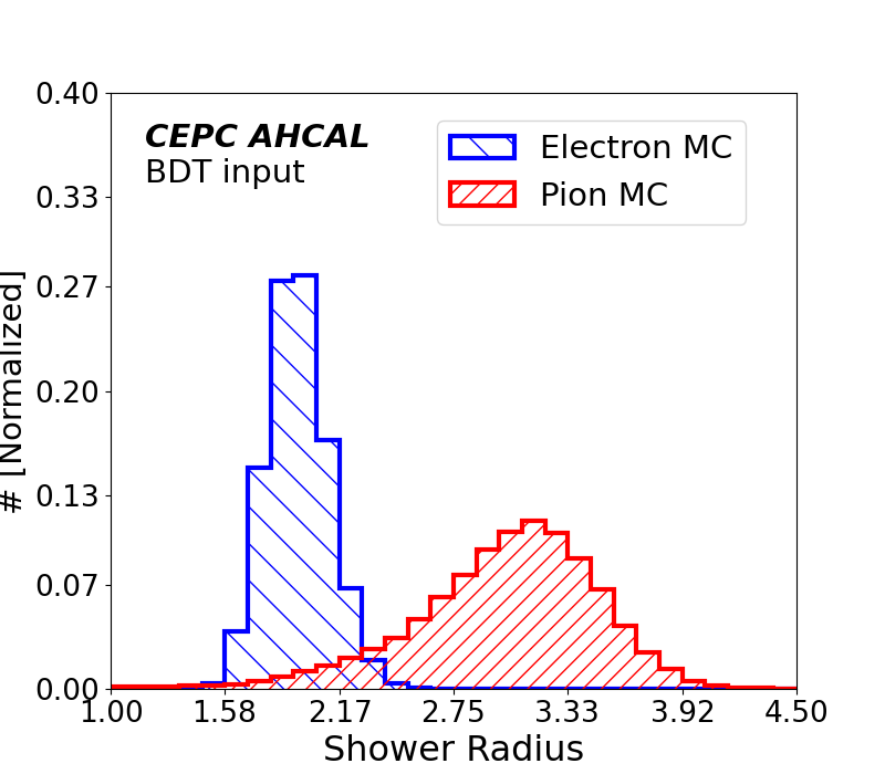
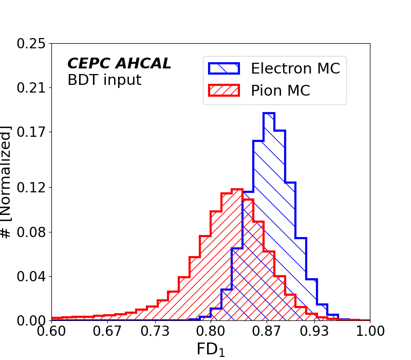
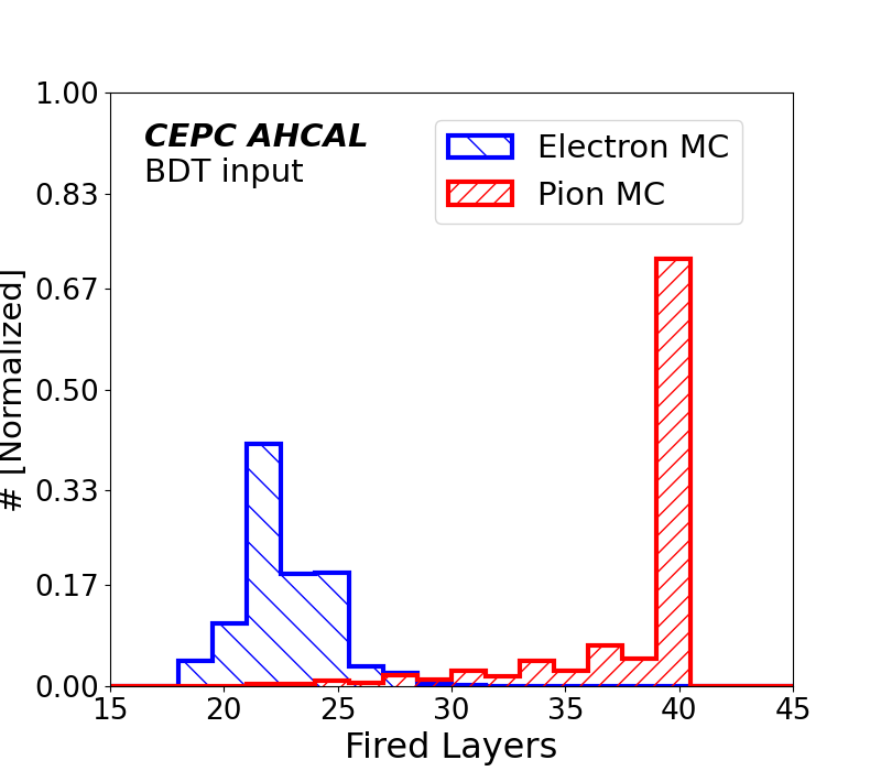
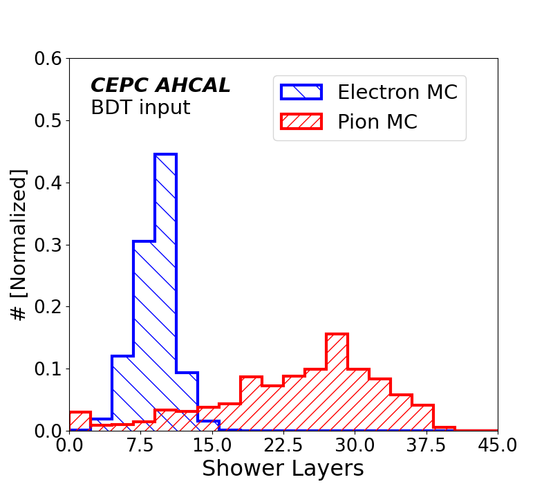
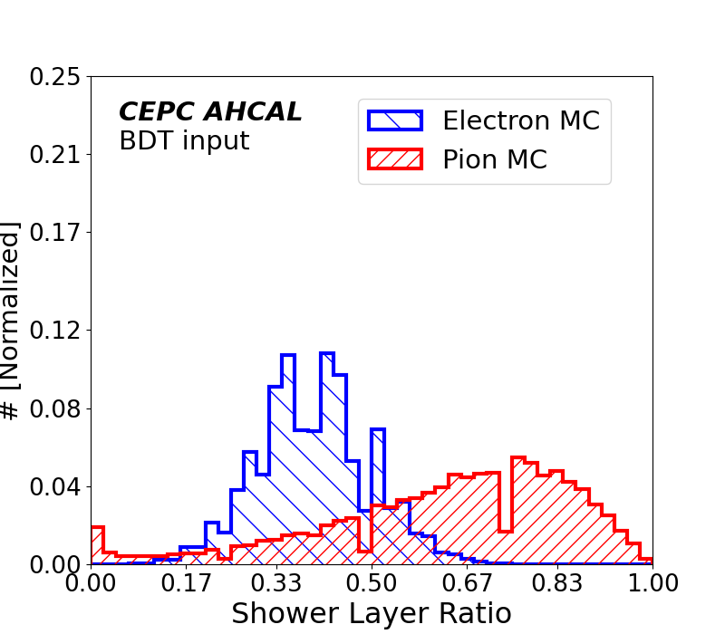
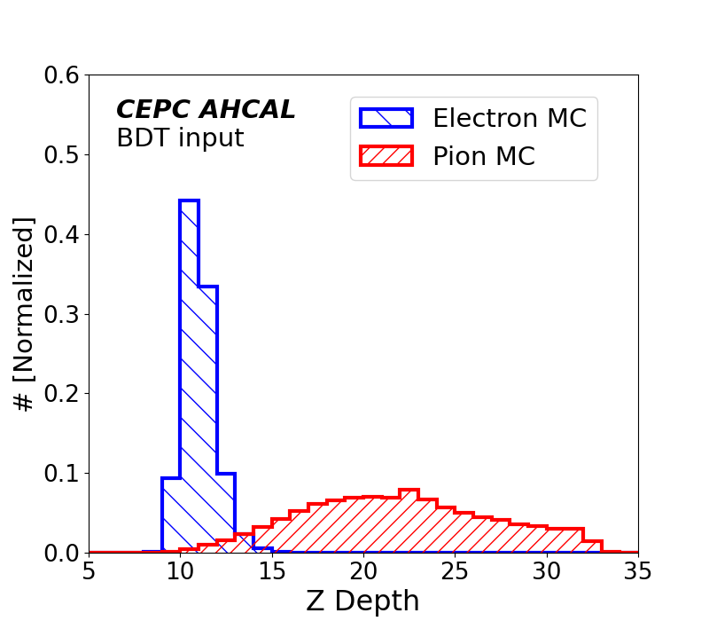
Figure 4: The distribution of the Shower Density (a), the Shower Start (b), the Shower End (c), the Shower Length (d), the Hits Number (e), the Shower Radius (f), the $\mathrm{FD}_{1}$ (g), the $\mathrm{FD}_{6}$ (h), the Fired Layers (i), the Shower Layers (j), the Shower Layer Ratio (k), and the Z Depth (l).

These 12 variables are utilized as inputs as they encapsulate characteristics of both electromagnetic and hadronic showers. The corresponding correlation matrix is depicted in figure 5. In this context, we consider pion events as signals and electron events as backgrounds. Our BDT classifier condenses these 12 reconstructed shower topology variables into BDT pion likelihoods ($L_{\pi}^{\mathrm{BDT}}$). It’s worth highlighting that among these variables, Z Depth and Shower Radius emerge as the two most crucial ones in terms of their separation power, as demonstrated in table 2.

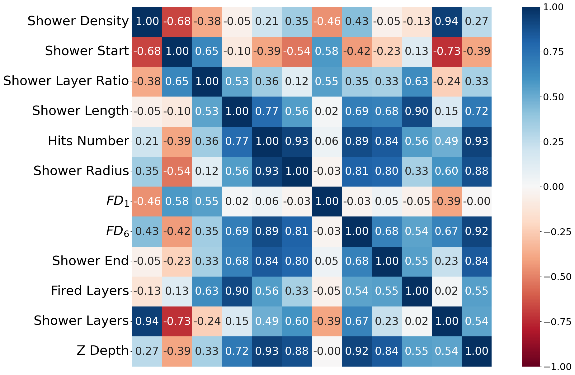
Figure 5: The correlation matrix of shower topology variables based on MC samples.

Table 2: Ranking of separation importance between electromagnetic showers and hadronic showers.

Rank: Variable	Variable weight
1: Z depth	0.532
2: Shower radius	0.186
3: Shower layers	0.073
4: Fired layers	0.065
5: Shower density	0.370
6: Shower start	0.026
7: Shower layer ratio	0.022
8: $\mathrm{FD_{1}}$	0.018
9: Hits number	0.013
10: $\mathrm{FD_{6}}$	0.012
11: Shower end	0.009
12: Shower length	0.006

3.1 BDT method performance

A higher BDT likelihood value indicates a more signal-like event. In figure 6, the output BDT likelihoods are presented using the MC test set. The values differ significantly for signal and background. This is confirmed in figure 6, through two metrics — the signal efficiency ($\varepsilon$) and the background rejection ($R$). These two metrics are inversely related. The signal efficiency represents the proportion of true signals correctly identified by classifiers, while the background rejection represents the ratio of total background numbers to the background mistakenly identified as signals. An effective classifier should keep both two metrics robust.

In our test set, each type of particle always occupies the same proportion. As reference points in pion identification, to achieve 99% pion signal efficiency ($\varepsilon_{\pi}$), the BDT pion likelihood ($L_{\pi}^{\mathrm{BDT}}$) should be over 0.1878, with corresponding 105 background rejection ($R_{e}$).

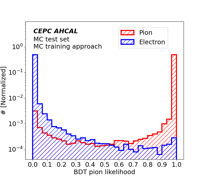
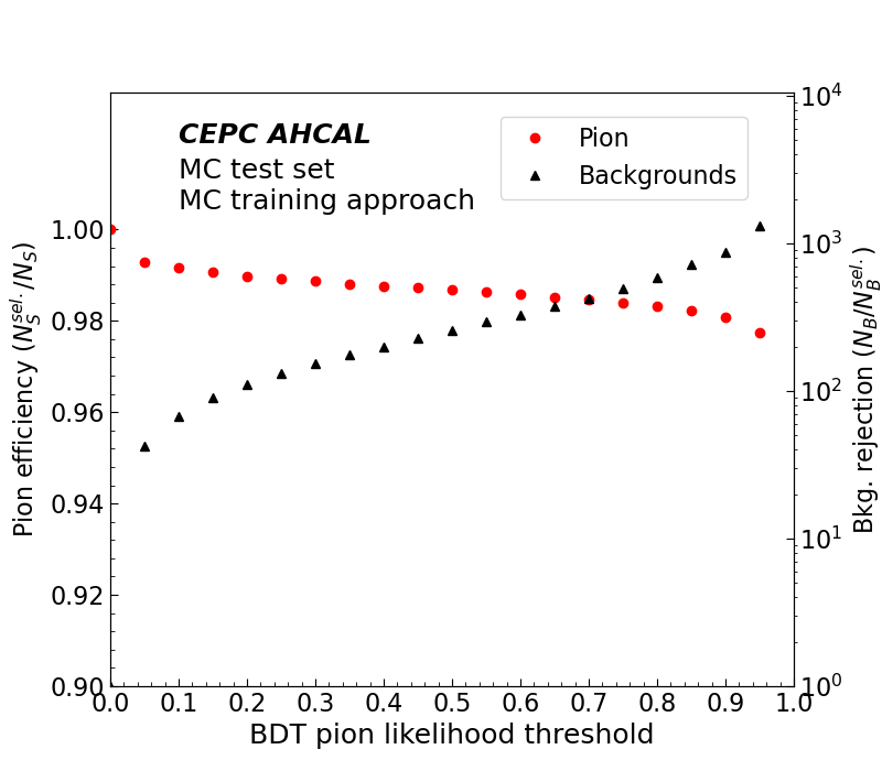
Figure 6: The distribution of the BDT pion likelihood (a). Pion efficiency and background rejection as the function of the BDT pion likelihood threshold (b).

3.2 Dependence of BDT performance on input variables

An ablation study is conducted to observe the dependence of BDT performance on input variables. Our original BDT classifier has 12 inputs. We first remove variables Shower End, Shower Layers, Fired Layers, and Z Depth, to build BDT with 8 inuts. We further remove variables $\mathrm{FD_{1}}$ and $\mathrm{FD_{6}}$, to build BDT with 6 inputs.

Figure 7 illustrates the obvious influence of variable numbers on BDT. When more variables are included, the performance of the BDT classifiers is improved, as the background rejection is higher almost at each signal efficiency point. We assume that the performance of the BDT classifier can be further improved when more meaningful shower topology variables are reconstructed. The further optimization of our BDT classifier is ongoing. In this paper, we only focus on providing a benchmark for our CEPC ResNet classifier.

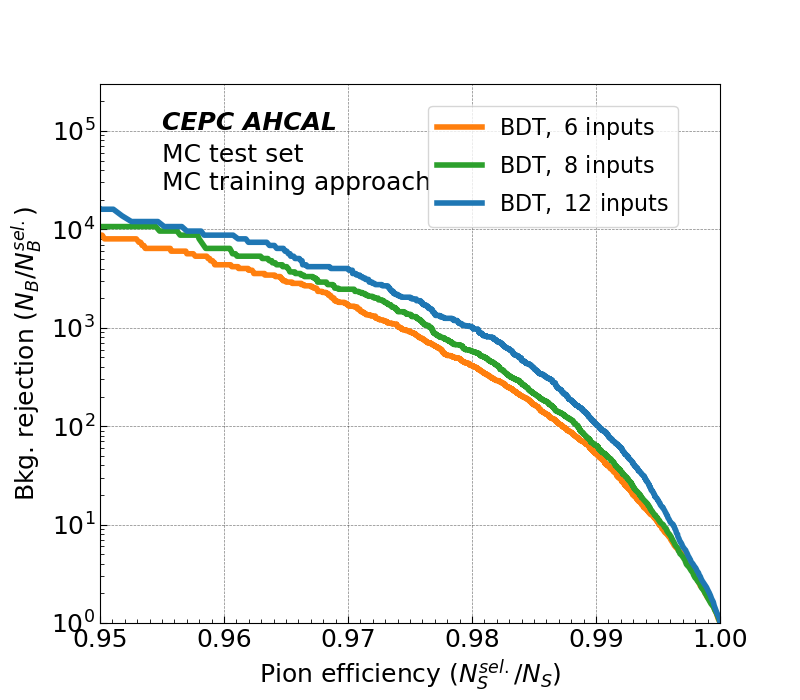
Figure 7: The comparison of BDT classifier with different input numbers in terms of background rejection versus signal efficiency in pion identification

4 PID based on ANN

4.1 Algorithm and architecture

ANN comprises multiple layers of interconnected nodes or “neurons” [26, 27]. The input layer receives a tensor. In the context of CEPC AHCAL, for each event, the energy depositions on the $40\times 18\times 18$ array of sensitive cells can be directly represented as the input tensor. It is then propagated through the multiple hidden layers with trainable parameters to the output layer, in which intermediate computations and non-linear transformations are made to extract useful features. The output of the ANN is a multi-class tensor $\hat{y}$ with $n$ values, where $n$ is the number of potential primary particle candidates. These values can be normalized using the Softmax function 4.1 [28], and interpreted as likelihoods for each candidate. By selecting the candidate with the highest likelihood value, the type of the primary particle is predicted [29].

$$\begin{split}&\sigma(\textbf{z})_{i}=\frac{e^{z_{i}}}{\sum_{j=1}^{n}e^{z_{j}}},\\ &\mathrm{for}\ i=1,...,n\ \mathrm{and}\ \textbf{z}=(z_{1},...,z_{n})\in\mathbb{R}^{n}.\end{split}$$ (4.1)

The structure and complexity of the network can be customized for different tasks [30, 31, 32]. We take the architecture of the ResNet with higher classification accuracies [13] as demonstrated in figure 8. Its generalization ability on unseen data has also been theoretically guaranteed [33]. The key idea behind ResNet is the use of residual blocks, which allow the network to learn residual mappings instead of trying to learn the direct mappings between the block’s input and output. A residual block consists of convolutional layers to extract features from the input and a shortcut connection, also known as a skip connection, that bypasses one or more layers. By propagating the identity mapping through the shortcut connection, ResNet enables the network to learn the residual mapping, capturing the difference between the input and output. In order to adapt it to the AHCAL prototype’s 40 sampling layers, the input channel number of the first convolution layer has been set to 40. Besides, as shown in figures 8, 8, 8, and 8, architectures in residual blocks have also been adjusted as more convolutional layers are included.

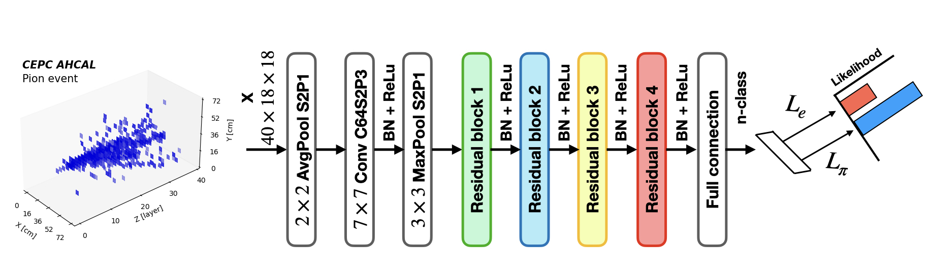
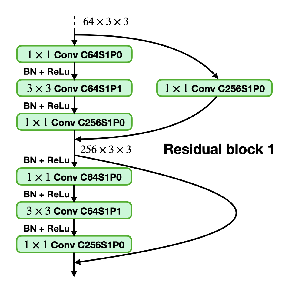
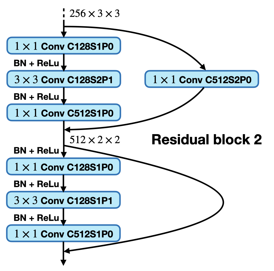
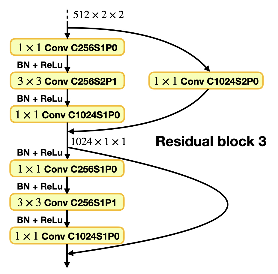
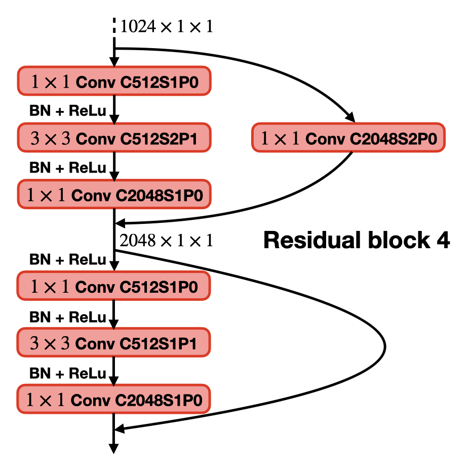
Figure 8: The schematic net architecture of CEPC ResNet PID. The output is a normalized tensor. The “Conv” indicates a 2D convolutional layer, and the “C” specifies the number of output channels. The “S” denotes the stride, which determines the step size for the convolution operation as the kernel moves over the input. The “P” represents the padding applied to the input. The “Maxpool” represents a max-pooling layer.

The trainable parameters are automatically adjusted during the training process to improve its ability to make accurate predictions. This adjustment is achieved by minimizing a loss function that quantifies the discrepancy between the network’s predicted outputs and the ground truth labels. In our PID method, we employ the categorical cross-entropy loss function [34], which is commonly used for image classification tasks and also suits our PID framework. The net’s prediction $\hat{y}_{i}$ serves as the input to the categorical cross-entropy loss function, which becomes a function of the network’s trainable parameters $\theta$. This relationship is expressed in equation 4.2. To optimize the values of $\theta$ and minimize the loss, we employ the Stochastic Gradient Descent (SGD) algorithm [35, 36, 37]. This process is outlined in Algorithm 1. Through this optimization process, the ResNet gradually learns to make more accurate predictions, improving its performance in particle identification tasks.

$$\mathrm{Loss}=\mathrm{Loss}\left({y}_{i},\hat{{y_{i}}}(\theta)\right)=-\sum_{i=1}^{n}y_{i}\log{\hat{y_{i}}(\theta)}$$ (4.2)

Algorithm 1 Artifical Neural Networks.

1:The batch size $m$, the epoch number $n$, initial learning rate $lr$, initial net parameters $\theta_{0}$.

2:Assign corresponding label $y$ to data $x$.

3:for $t=1,\cdots,k$ iteration steps  do

4:     for $i=1,\cdots,m$ do

5:         $\hat{y}\leftarrow\mathrm{Net}(x,\theta)$

6:         $\mathrm{Loss}({y}_{i},\hat{{y_{i}}})_{\theta}^{(i)}\leftarrow(-\mathrm{log}(\hat{{y_{i}}}))$

7:     end for

8:     $\theta\leftarrow\mathrm{SGD}\left(\bigtriangledown_{\theta}\frac{1}{m}\sum_{i=1}^{m}\mathrm{Loss}_{\theta}^{(i)}\right)$

9:end for

To train ANN, including ResNet, the total iteration steps $k$ equals $N\times{n}/m$, where $N$ is the number of events for training, $m$ is the batch size, and $n$ is the epoch number. The neural network is executed on an NVIDIA V100 NVLink GPU, utilizing the NVIDIA CUDA platform. The code is scripted in Python and employs the PyTorch deep learning library [38]. Due to resource constraints, conducting an exhaustive exploration of hyper-parameters was not feasible. However, we still tested hundreds of hyper-parameter combinations, repeated the training 10 times with different initial weights to mitigate the impact of fluctuations resulting from different initializations, and finally selected the one that yielded the best performance (highest classification accuracy). We decided the batch size $m$ to be 64, the epoch number $n$ to be 200, and the initial learning rate $lr$ to be $1\times 10^{-4}$.

4.2 Impacts of the Residual Connections

In our experiment, the efficacy of the Residual Connections was first validated by comparing the error ($\frac{N_{misclassified}}{N_{total}}\times$100%) during iterations with and without the Residual Connections shortcut. When the network operated without the shortcut, our ResNet classifier became non-residual. Figure 9 illustrates the impact of the shortcut connection across various combinations of batch sizes (64,  128,  256 ) and learning rates ($1\times 10^{-5}$, $1\times 10^{-4}$, $1\times 10^{-3}$) while maintaining 200 epochs.

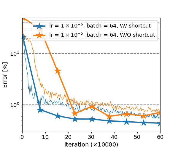
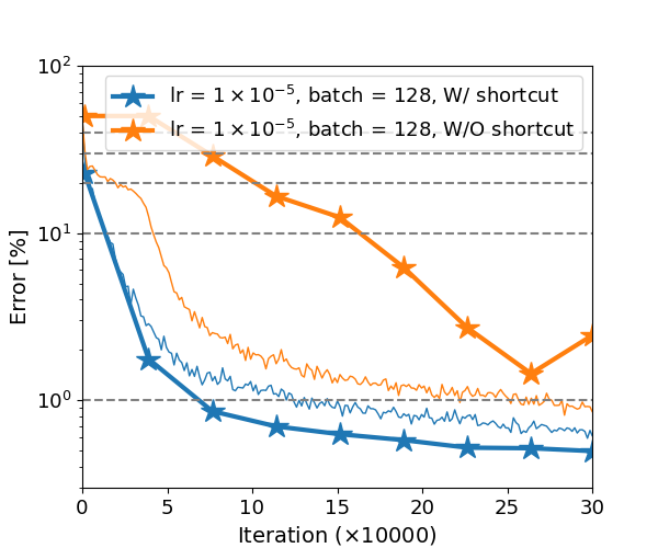
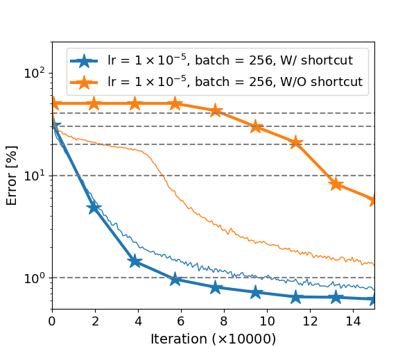
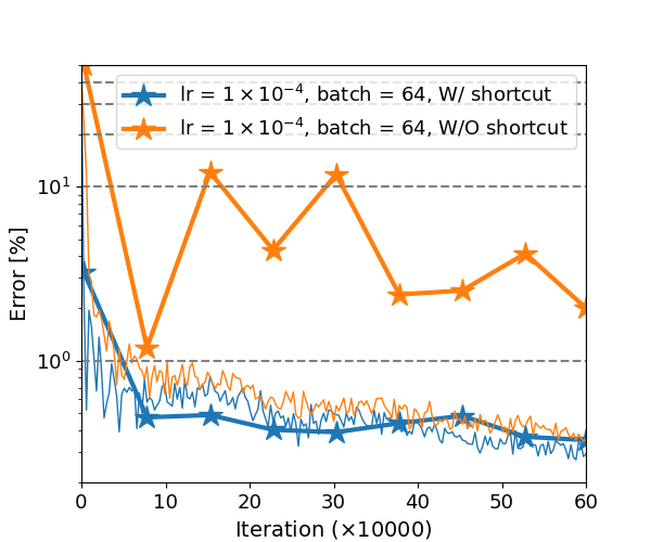
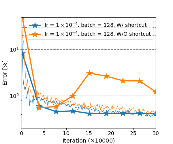
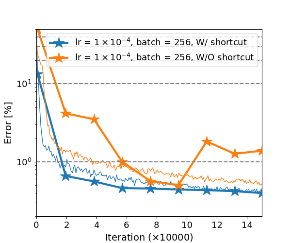
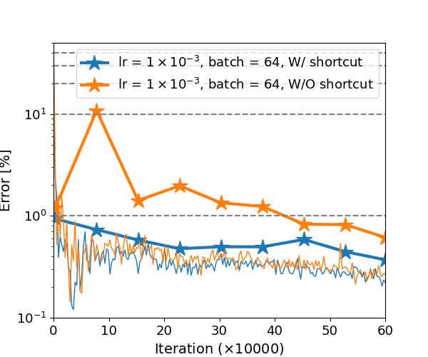
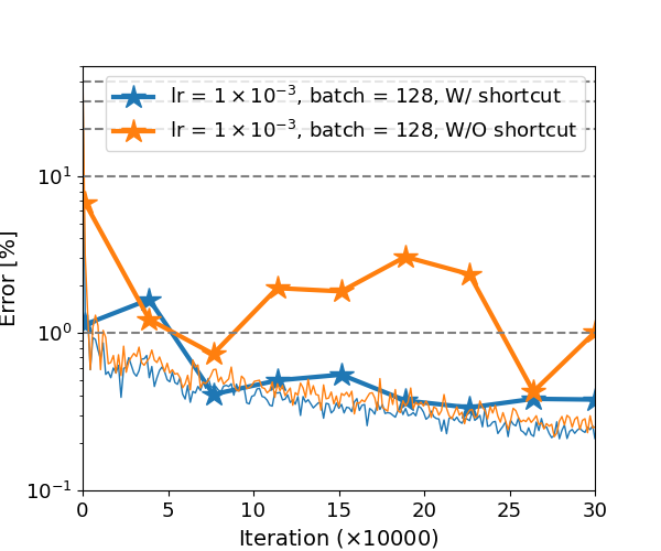
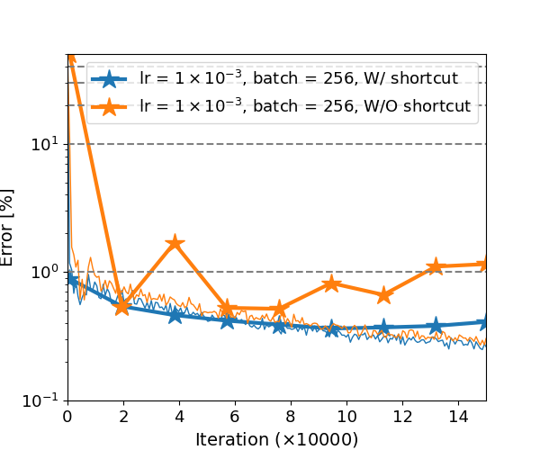
Figure 9: Training the ResNet classifier involves adjusting the learning rate ($lr$), set at $1\times 10^{-5}$ in the first row, $1\times 10^{-4}$ in the second row, and $1\times 10^{-3}$ in the third row. Additionally, the batch size varies across three configurations: 64 (left), 128 (middle), and 256 (right). In the plot, thin curves represent the training error, while bold curves depict the validation error. The training error is updated after each epoch, and the validation error is updated every 25 epochs using the independent validation set. Notably, the only distinction in the same plot lies in the presence or absence of shortcuts.

Notably, the number of iterations per epoch varies, with 3000 iterations per epoch for a batch size of 64, 1500 iterations per epoch for a batch size of 128, and 750 iterations for a batch size of 256. In our experiments, under the optimized combination of hyper-parameters, as shown in the upper left sub-figure 9, the existence of the shortcut connection led to a faster decrease in both training and validation errors during the initial few epochs.

Moreover, it tends to mitigate the fluctuation of the validation error, also observed across other combinations of batch size and learning rate, consistent with findings in the reference paper [13]. Table 3 lists the validation error (%) recalculated after 200 epochs of iterations using the validation set with various combinations of batch size and learning rate. Under the optimized combination of learning rate and batch size, the validation error is at its lowest, standing at 0.35%. Introducing the shortcut connection results in a reduction of the validation error by a factor of 2-3 in most cases of our experiments. These results suggest that the existence of the shortcut can enhance the robustness of the network and should be employed in our model.

Table 3: The validation error (%) was recalculated after 200 epochs’ iterations using the validation set. Keeping the learning rate and batch size constant, the only distinction lies in the presence or absence of the shortcut. The training procedures are illustrated in figure 9.

	W/ shortcut	W/O shortcut
$lr$ = $1\times 10^{-5}$, batch = 64	0.441	0.716
$lr$ = $1\times 10^{-5}$, batch = 128	0.497	2.445
$lr$ = $1\times 10^{-5}$, batch = 256	0.621	5.789
$lr$ = $1\times 10^{-4}$, batch = 64	0.350	2.009
$lr$ = $1\times 10^{-4}$, batch = 128	0.407	1.220
$lr$ = $1\times 10^{-4}$, batch = 256	0.397	1.385
$lr$ = $1\times 10^{-3}$, batch = 64	0.371	0.615
$lr$ = $1\times 10^{-3}$, batch = 128	0.378	1.015
$lr$ = $1\times 10^{-3}$, batch = 256	0.409	1.156

4.3 ResNet performance

Electron events and pion events in the test set occupy the same proportion. Figure 10 shows the pion likelihood distribution. It can be observed that a significant separation power has been achieved as well. For example, in figure 10, pion events tend to have higher values in the pion likelihood compared to electron events, indicating that the ResNet is capable of distinguishing pions from electrons. This observation is further supported by figure 10. At the same target pion efficiency ($\varepsilon_{\pi}$) of 99%, the ResNet achieves an electron background rejection ($R_{e}$) of approximately 2000, where the ResNet pion likelihood ($L_{\pi}^{\mathrm{ResNet}}$) should be over 0.9037.

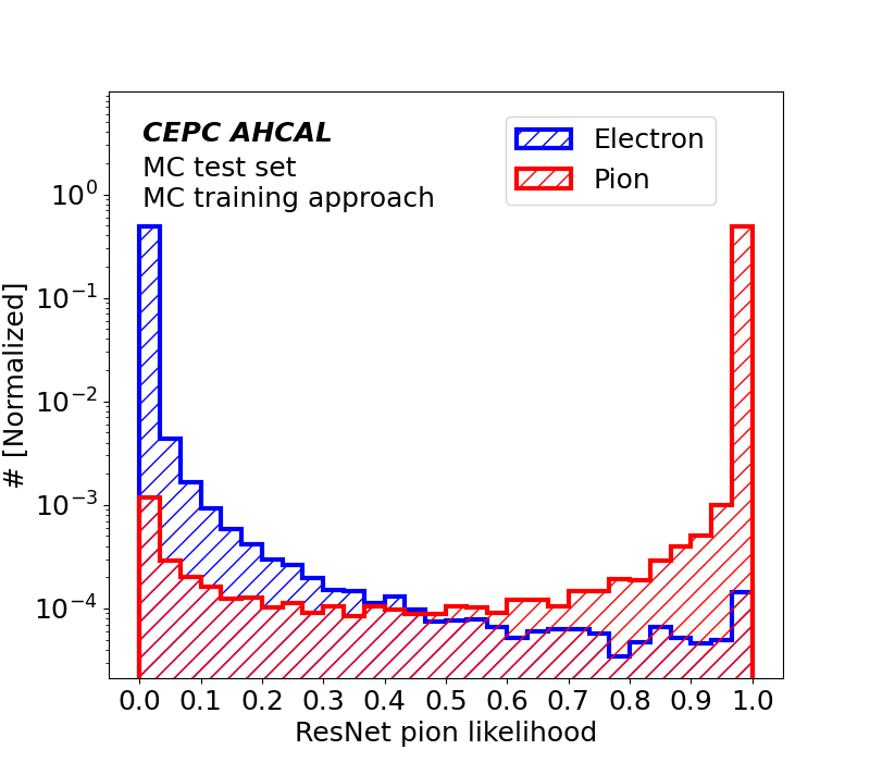
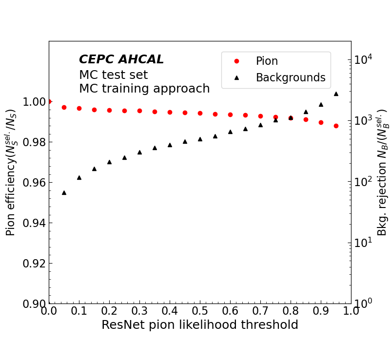
Figure 10: The distribution of the ResNet pion likelihood (a). Pion efficiency and background rejection as the function of the ResNet pion likelihood threshold (b).

Moreover, our ResNet classifier is compared with the aforementioned BDT classifier (utilizing 12 input variables), as well as with LeNet[19], one of the earliest CNN, and AlexNet[14], once achieving remarkable performance on the ImageNet Large Scale Visual Recognition Challenge (ILSVRC). It is noteworthy that all neural network models undergo an identical hyper-parameter optimization process, and the training is iterated 10 times with varying randomly initialized weights to evaluate stability. The combination of hyper-parameters (batch size, learning rate) is (32, $1\times 10^{-3}$) for AlexNet and (256, $1\times 10^{-5}$) for LeNet. Figure 11 presents the comparison in terms of electron background rejection at the same pion signal efficiency and table 4 summarizes the corresponding key metrics with physics insights including electron rejection ($R_{e}$) at a certain pion efficiency ($\varepsilon_{\pi}$) of 97%, 98%, 99%, and 99.5%, and the classification accuracy. We observe that the ResNet classifier tailored by our team demonstrates superior performance. For instance, at $\varepsilon_{\pi}$ of 99%, The ResNet classifier markedly enhances $R_{e}$ by a factor of 20, increasing it from approximately 100 to about 2000. Furthermore, when $\varepsilon_{\pi}$ equals 97%, ResNet’s $R_{e}$ capability surpasses that of AlexNet and LeNet by roughly 1.5 times, and it even outperforms BDT by an impressive factor of 5.

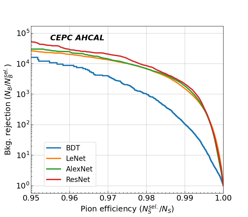
Figure 11: The comparison of background rejection versus signal efficiency for BDT, LeNet, AlexNet, and ResNet in identifying pions against electron backgrounds, with results computed from the test set.

Table 4: PID performance of BDT, AlexNet, LeNet, and ResNet on pion identification, evaluated using the test set. The training of BDT is performed only once since the uncertainty of BDT due to random weight initialization is expected to be fairly small. The training of other models is repeated 10 times using different randomly initialized weights. The table shows the mean value and the standard error of electron background rejection ($R_{e}$) and classification accuracy to assess the stability to random weight initialization. The uncertainty of the classification accuracy of LeNet is also found to be negligible.

	$R_{e}^{\varepsilon=97\%}$	$R_{e}^{\varepsilon=98\%}$	$R_{e}^{\varepsilon=99\%}$	$R_{e}^{\varepsilon=99.5\%}$	Accuracy [%]
BDT	4003	1011	105	18	99.15
AlexNet	14260 $\pm$ 223	6791 $\pm$ 73	1864 $\pm$ 36	323 $\pm$ 7	99.45 $\pm$ 0.04
LeNet	13427 $\pm$ 163	6933 $\pm$ 49	1514 $\pm$ 19	314 $\pm$ 4	99.43
ResNet	23576 $\pm$ 202	8547 $\pm$ 85	2165 $\pm$ 45	356 $\pm$ 6	99.61 $\pm$ 0.02

4.4 Prospects in point cloud scenarios

Our ResNet PID model currently relies on detectors with regular structures to construct image-based inputs, though the AHCAL prototype exhibited normal structures, making it a natural choice to employ 2D-convolution-based deep learning methods. However, it is important to note that the geometry of detectors is not universally confined to cubic structures with fixed tile sizes. For example, detectors utilized in collider experiments, both existing and future ones[39, 40, 41, 42], often adopt a barrel-like configuration with variable tile sizes, to maximize the chances of detecting particles produced in the collision. The upgraded design of the AHCAL in the future would probably not be limited to fixed tile size as well. Therefore, this might pose challenges to the application prospect of our algorithm.

Actually, 3D shapes could also be represented in the point clouds, characterized by their permutation invariance and the flexibility to incorporate diverse features for each point. This approach ensures that the representation of showers is not constrained by the geometry of detectors, thereby showcasing its versatility as an input method. Here, we propose a tailored solution to point cloud scenarios based on the current ResNet model, called the Dynamic Graph Residual Networks (DGRes).

Traditional approaches to processing point clouds typically rely on handcrafted features to capture their geometric properties [43, 44]. Recently, advancements in deep point cloud processing methods by leveraging deep neural networks have been made. These data-driven methods excel in learning features and have demonstrated superior performance compared to traditional techniques across a spectrum of tasks [45, 46]. DGRes is inspired by the Dynamic Graph Convolutional Neural Networks (DGCNN)[15], which introduces graph convolution, namely the EdgeConv, to explore structural information between points. Figure12 illustrates the fundamental concept of EdgeConv, which involves treating points themselves as vertices ($v_{i}$), with edges established as connections between dynamically changed $k$ nearest neighboring vertices, determined by the k-nearest neighbor (kNN) algorithm [47]. The same formulation of EdgeConv from the referenced paper [15] was adopted in our model:

$$\mathbf{v}_{i}^{\prime}=\underset{j:(i,j)\in\mathcal{E}}{\operatorname*{\mathrm{max}}}e_{ij}=\underset{j:(i,j)\in\mathcal{E}}{\operatorname*{\mathrm{max}}}{\bar{h}_{\Theta}(\mathbf{v}_{i},\mathbf{v}_{j}-\mathbf{v}_{i})}.$$ (4.3)

The $\mathbf{V}=\{\mathbf{v}_{1},\ldots,\mathbf{v}_{q}\}\subseteq\mathbb{R}^{F}$ denotes $q$ vertices in the cloud with features, $e_{ij}$ is the edge feature, and $\bar{\bm{h}}_{\Theta}$ is realized as a multilayer perceptron (MLP) with shared parameters across all edges. Consequently, the DGRes architecture (shown in figure 13) can be delineated into two components: the initial segment comprises conversion layers based on EdgeConv, facilitating the transformation of point-cloud-based (graph-based) data into image-based data, represented in a reconstructed three-dimensional space. The subsequent part involves the ResNet architecture, which is discussed in subsection 4.3 to extract features and classify events.

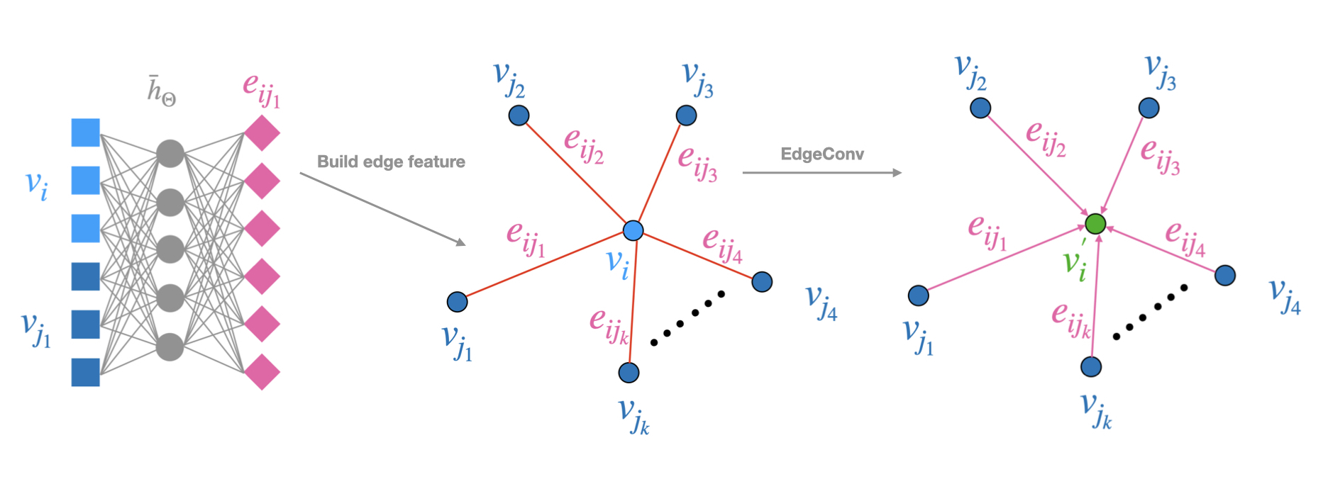
Figure 12: The schematic plot illustrates the functionality of the EdgeConv block. In this example, the edge feature $e_{ij_{1}}$ is computed from a pair of vertices, $v_{i}$ and $v_{j_{1}}$, by instantiating $\bar{h}_{\Theta}$ with a fully connected layer to map ($v_{i}$, $v_{j_{1}}$-$v_{i}$) into $e_{ij_{1}}$. The output of EdgeConv, denoted as $v_{i}^{\prime}$, is calculated by aggregating the edge features associated with k nearest vertices.

A comparative analysis was conducted involving our DGRes and two baseline algorithms: DGCNN and GravNet. DGCNN has been already introduced above. The GravNet employs distance-weighted graph networks, originally proposed for tasks such as cluster reconstruction and particle identification [16]. The integration of GravNet has resulted in the formulation of an end-to-end reconstruction algorithm tailored for the single-shot calorimetric reconstruction of approximately 1000 particles. This is particularly crucial in high-luminosity conditions with 200 pileups [17].

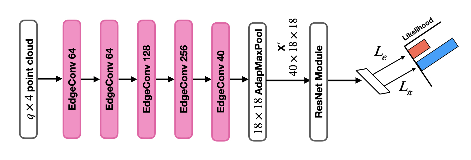
Figure 13: The architecture of DGRes. Conversion layers based on EdgeConv take point-cloud-based data as input and map them into tensors with 3 dimensions (shape: $40\times 18\times 18$), which could be processed by the ResNet module illustrated in figure 8.

All models undergo training and testing using the identical set of feature vectors pre-reconstructed from the dataset introduced in Section 2. Feature vectors $v_{i}=~{}(x_{i},y_{i},z_{i},e_{i})$ represent the coordinates of hits and the corresponding deposited energy. Training is consistently conducted over 200 epochs. To accommodate variations in the Hits Number for each event, we make $q$, the number of vertices, as a hyper-parameter during training to facilitate efficient mini-batch training. When the Hits Number exceeds $q$, we randomly select $q$ different hits from all hits to form vertices to create a sub-graph in each iteration. Conversely, if the Hits Number is smaller than $q$, features of the empty vertices are padded with zeros. Given that electromagnetic showers and hadronic showers exhibit distinct local structures, the number of nearest neighboring vertices, $k$, can be interpreted as a local connection scale for hits in showers. The effectiveness of models in capturing local structures is influenced by the specific value of $k$, making it another hyper-parameter to be optimized.

For DGCNN, we utilize an existing PyTorch implementation. In the case of GravNet, we re-implement the network architecture originally for the reconstruction task, as outlined in the paper [17], into PyTorch for classification. The combination of parameters (batch size, learning rate, number of vertices, number of nearest neighboring vertices) is re-optimized, resulting in (32, 0.01, 256, 10) for DGRes, (128, 0.1, 128, 20) for DGCNN, and (32, $1\times 10^{-3}$, 256, 10) for GravNet. The performance evaluation utilizes identical metrics with physics insights outlined in subsection 4.3. Figure 14 depicts the electron background rejection versus the pion signal efficiency of DGRes, DGCNN, and GravNet. Moreover, this comparison encompasses AlexNet, LeNet, BDT, and ResNet, providing a comprehensive overview of all models, with corresponding results summarized in table 5.

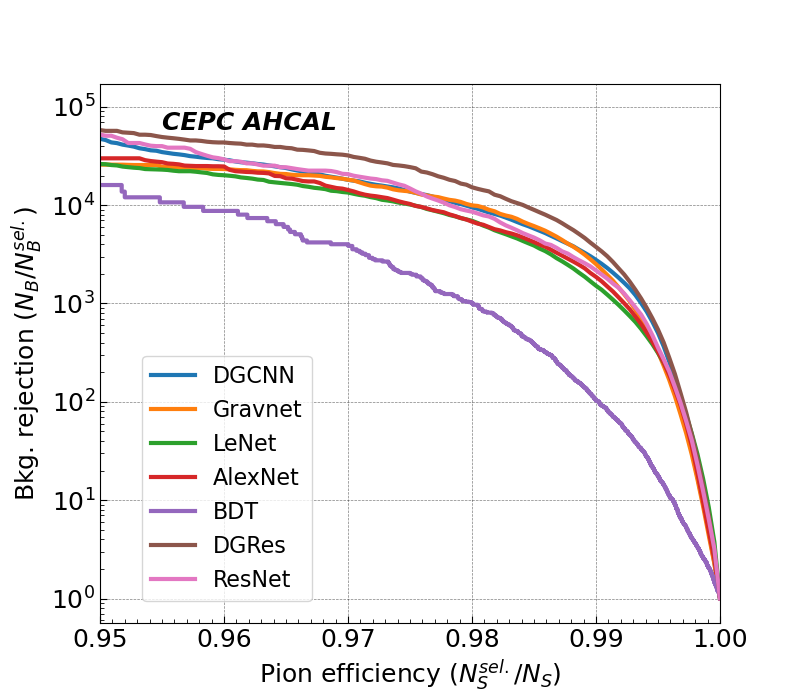
Figure 14: The comparison of background rejection versus signal efficiency for DGCNN, GravNet, and DGRes, together with BDT, LeNet, AlexNet, and ResNet, in identifying pions against electron backgrounds, with results computed from the test set.

Notably, the DGRes model demonstrates superior performance across all metrics. Specifically, DGRes achieves a background rejection of 3758, surpassing GravNet and DGCNN by approximately a factor of 1.5 when the signal efficiency ($\varepsilon_{\pi}$) is set at 99%. This superior performance can be attributed to the utilization of ResNet with deeper networks following several EdgeConv blocks in our DGRes model, which expands the parameter space, promising enhanced performance. Additionally, the effectiveness of EdgeConv blocks in capturing features and transforming point cloud data into image-based data is evident from the improved performance of DGRes compared to purely image-based ResNet, such as improving the electron background rejection by a factor of 1.7 at 99% signal efficiency. Consequently, These findings indicate promising prospects for the application of our PID method, even in scenarios where tile sizes vary.

Table 5: PID performance of DGRes is compared to GravNet and DGRes on pion identification, evaluated using the test set. The training of each model is repeated 10 times using different randomly initialized weights. The table shows the mean value and the standard error of electron background rejection ($R_{e}$) and classification accuracy to assess the stability to random weight initialization. The uncertainty of classification accuracy of DGCNN and DGRes is found to be negligible. The performance of BDT, AlexNet, LeNet, and ResNet listed in table 4 is also provided.

	$R_{e}^{\varepsilon=97\%}$	$R_{e}^{\varepsilon=98\%}$	$R_{e}^{\varepsilon=99\%}$	$R_{e}^{\varepsilon=99.5\%}$	Accuracy [%]
DGCNN	18085 $\pm$ 289	9498 $\pm$ 102	2772 $\pm$ 46	501$\pm$ 6	99.65
GravNet	18127 $\pm$ 227	9942 $\pm$ 88	2516 $\pm$ 34	321 $\pm$ 4	99.47 $\pm$ 0.08
DGRes	32011 $\pm$ 204	15193 $\pm$ 116	3758 $\pm$ 20	543 $\pm$ 6	99.71
BDT	4003	1011	105	18	99.15
AlexNet	14260 $\pm$ 223	6791 $\pm$ 73	1864 $\pm$ 36	323 $\pm$ 7	99.45 $\pm$ 0.04
LeNet	13427 $\pm$ 163	6933 $\pm$ 49	1514 $\pm$ 19	314 $\pm$ 4	99.43
ResNet	23576 $\pm$ 202	8547 $\pm$ 85	2165 $\pm$ 45	356 $\pm$ 6	99.61 $\pm$ 0.02

4.5 Model complexity

The computational cost stands as another crucial factor in model evaluation. The table 6 outlines various metrics including the number of parameters, model size, training time for one epoch (the batch size of each model varies based on optimization results), inference time for one event (using a batch size of 256), and electron background rejection $R_{e}$ ($\varepsilon_{\pi}$ = 99%) for each ANN-based model, all computed using a single NVIDIA V100 NVLink GPU.

Although our ResNet-based classifier and the upgraded version, the DGRes which works on point cloud scenarios, are built in one order of magnitude higher parameters, they perform better in terms of $R_{e}$ in image cases and graph cases respectively, without resulting in an order of magnitude higher training and inference costs. Furthermore, the ResNet model based on image data exhibits a quite short inference time (1.45 ms) compared with graph-based approaches, which should be attributed to the benefits of the optimized parallel processing capabilities of the GPU operating on tensors. In contrast, graph-based networks in our study are influenced by factors such as the number of nodes and nearest neighboring points as we must dynamically construct edge connections and features, which were currently not optimized for parallel processing. The relatively higher time cost associated with DGRes and GravNet can also be attributed to their requirement for a greater number of vertices (256) to construct a sub-graph during each iteration, based on our optimization findings.

Table 6: Number of parameters, model size, electron background rejection ($\varepsilon$ = 99%, uncertainty is not listed), training time for one epoch, and inference time for one event of different models. Training and inference time are recorded using a single NVIDIA V100 NVLink GPU. For training, DGCNN employs a batch size of 128, GravNet utilizes a batch size of 32, AlexNet takes a batch size of 32, LeNet employs a batch size of 256, DGRes adopts a batch size of 32, while ResNet employs a batch size of 64, with optimal performance in background rejection. Inference time for all models is computed using a batch size of 256.

	Parameters	Model size	$R_{e}^{\varepsilon=99\%}$	Training [s/epoch]	Inference [ms/event]
DGCNN	$1.8\times 10^{6}$	6.87 MB	2772	99.96	2.69
GravNet	$3.4\times 10^{6}$	13.02 MB	2516	624.11	12.60
AlexNet	$5.7\times 10^{7}$	217.48 MB	1864	51.55	1.56
LeNet	$6.7\times 10^{6}$	25.41 MB	1514	13.67	0.71
DGRes	$1.4\times 10^{7}$	53.92 MB	3758	338.31	4.89
ResNet	$1.4\times 10^{7}$	53.66 MB	2165	105.41	1.45

The training and inference performance of ResNet, DGRes, DGCNN, and GravNet with batch sizes ranging from 32 to 256 is further investigated as shown in figure 15. Here, the inference time is calculated by event. Notably, we observe that ResNet (image-based) experiences the most significant benefit from the optimized parallel processing capabilities of the GPU. This is evidenced by the time cost for training and inference gradually becoming the lowest compared with other models when the batch size keeps increasing to 256, consistent with the feature of parallel processing. Consequently, this presents a disadvantage, particularly during large-batch inference in applications.

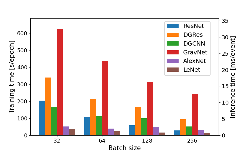
Figure 15: The training and inference time with a variation of batch size.

4.6 Discussion

Firstly, ANN provides a powerful framework for learning from data, with CNN excelling in processing grid-like data such as images, and GNN being specialized for handling graph-structured data as we observe that all ANN classifiers (ResNet, DGRes, DGCNN, GravNet, LeNet, ALexNet) outperform our BDT classifier in pion identification, which should be attributed to the advantage of ANN in harnessing the rich information present in high-dimensional inputs. Conversely, the intricate nature of electromagnetic and hadronic showers poses challenges for TMVA BDT, as it struggles to capture the complete shower details with a limited set of feature variables. Applying BDT is more akin to employing human-like thinking since it depends on pre-reconstructed human-readable variables. It is also possible that our BDT will be further improved if more shower topology variables are reconstructed, but conducting this feature engineering would sometimes be tricky.

Secondly, when applying ANN classifiers, both image-based and graph-based representations offer distinct advantages. In the case of image-based representation, image data can be high-dimensional, resulting in increased computational complexity and memory requirements, particularly for large datasets. Moreover, image-based classifiers may encounter challenges in generalizing well to variations in the geometry of detectors. However, they can effectively leverage the parallel processing capabilities of GPUs, enhancing computational efficiency. Conversely, graph-based data offers enhanced flexibility in accommodating varying numbers of features and adapting to changes in the geometry of detectors. Nevertheless, analyzing graph-based data can be computationally demanding, particularly for large graphs containing numerous nodes and edges. This complexity arises from the necessity to propagate information throughout the entire graph structure.

5 Conclusion

Novel PID methods based on Residual Artificial Neural Networks (ResNet) architecture are proposed to classify electron and hadron events based on the shower topology in high-granularity calorimeters, whose effectiveness is validated by using Monte Carlo simulation samples.

When classifying complex varieties of electromagnetic showers and hadronic showers, the introduction of the Residual Connection shortcut improves the robustness of neural networks. It also leads to superior performance, demonstrated in signal efficiency and background rejection, when image-based ResNet is compared with the BDT classifier, which relies on a limited input variable number and still has room for improvement when additional relevant variables are deliberately developed. We also offer a model called DGRes, an upgrade to ResNet, by leveraging multiple EdgeConv blocks to address the application limitation when the detector’s tile size is not fixed. In this scenario, data can initially be represented in point clouds (graph-based), allowing for flexibility regardless of the detector’s geometry. When compared with other state-of-the-art classifiers such as DGCNN and GravNet, our approach consistently demonstrates superior performance in electron background rejection.

As a result, our PID methods are practical, robust, feasible, efficient, and reliable in various imaging detectors with a huge amount of spatial information.

References

- [1] CEPC Study Group, CEPC Conceptual Design Report: Volume 2 — Physics & Detector, arXiv:1811.10545 (2018) .
- [2] A. Hoecker, P. Speckmayer, J. Stelzer, J. Therhaag, E. von Toerne, H. Voss et al., TMVA — Toolkit for Multivariate Data Analysis, arXiv: physics/0703039v5 (2007) .
- [3] B. Liu, I. Laktineh, Q. Shen, G. Garillot, J. Guo, F. Lagarde et al., Particle Identification Using Boosted Decision Trees in the Semi-Digital Hadronic Calorimeter, Journal of Instrumentation 15 (2020) C05022.
- [4] H.-J. Yang, B.P. Roe and J. Zhu, Studies of Boosted Decision Trees for MiniBooNE Particle Identification, Nuclear Instruments and Methods in Physics Research Section A: Accelerators, Spectrometers, Detectors and Associated Equipment 555 (2005) 370.
- [5] B.P. Roe, H.-J. Yang, J. Zhu, Y. Liu, I. Stancu and G. McGregor, Boosted Decision Trees as an Alternative to Artificial Neural Networks for Particle Identification, Nuclear Instruments and Methods in Physics Research Section A: Accelerators, Spectrometers, Detectors and Associated Equipment 543 (2005) 577.
- [6] B.P. Roe, H.-J. Yang and J. Zhu, Boosted Decision Trees, a Powerful Event Classifier, in Statistical Problems in Particle Physics, Astrophysics and Cosmology, L. Lyons and M.K. Ünel, eds., pp. 139–142, World Scientific (2006), .
- [7] S. Macaluso and D. Shih, Pulling out All the Tops with Computer Vision and Deep Learning, Journal of High Energy Physics 2018 (2018) 1.
- [8] F. Carminati, G. Khattak, M. Pierini, A. Farbin, B. Hooberman, W. Wei et al., Calorimetry with Deep Learning: Particle Classification, Energy Regression, and Simulation for High-Energy Physics, in Workshop on Deep Learning for Physical sciences (DLPS 2017), NIPS, (Long Beach), 2017, https://dl4physicalsciences.github.io/files/nips_dlps_2017_15.pdf.
- [9] D. Bourilkov, Machine and Deep Learning Applications in Particle Physics, International Journal of Modern Physics A 34 (2019) 1930019.
- [10] F. Psihas, M. Groh, C. Tunnell and K. Warburton, A Review on Machine Learning for Neutrino Experiments, International Journal of Modern Physics A 35 (2020) 2043005.
- [11] A.N. Charan, Particle Identification with the Belle II Calorimeter Using Machine Learning, Journal of Physics: Conference Series 2438 (2023) 012111.
- [12] A. Tumasyan, W. Adam, J.W. Andrejkovic, T. Bergauer, S. Chatterjee, M. Dragicevic et al., Identification of Hadronic Tau Lepton Decays Using a Deep Neural Network, Journal of Instrumentation 17 (2022) 53.
- [13] K. He, X. Zhang, S. Ren and J. Sun, Deep Residual Learning for Image Recognition, in 2016 IEEE Conference on Computer Vision and Pattern Recognition (CVPR), pp. 770–778, 2016, https://doi.org/10.1109/CVPR.2016.90.
- [14] A. Krizhevsky, I. Sutskever and G.E. Hinton, Imagenet classification with deep convolutional neural networks, Advances in neural information processing systems 25 (2012) .
- [15] Y. Wang, Y. Sun, Z. Liu, S.E. Sarma, M.M. Bronstein and J.M. Solomon, Dynamic graph cnn for learning on point clouds, ACM Transactions on Graphics (tog) 38 (2019) 1.
- [16] S.R. Qasim, J. Kieseler, Y. Iiyama and M. Pierini, Learning representations of irregular particle-detector geometry with distance-weighted graph networks, The European Physical Journal C 79 (2019) 1.
- [17] S.R. Qasim, N. Chernyavskaya, J. Kieseler, K. Long, O. Viazlo, M. Pierini et al., End-to-end multi-particle reconstruction in high occupancy imaging calorimeters with graph neural networks, The European Physical Journal C 82 (2022) 753.
- [18] T. Chen and C. Guestrin, XGBoost: A Scalable Tree Boosting System, in Proceedings of the 22nd ACM SIGKDD International Conference on Knowledge Discovery and Data Mining, (New York), pp. 785–794, Association for Computing Machinery, 2016, https://doi.org/10.1145/2939672.2939785.
- [19] Y. LeCun, L. Bottou, Y. Bengio and P. Haffner, Gradient-based learning applied to document recognition, Proceedings of the IEEE 86 (1998) 2278.
- [20] L. Li, Q. Shan, W. Jia, B. Yu, Y. Liu, Y. Shi et al., Optimization of the CEPC-AHCAL Scintillator Detector Cells, Journal of Instrumentation 16 (2021) P03001.
- [21] Y. Duan, J. Jiang, J. Li, L. Li, S. Li, D. Liu et al., Scintillator Tile Batch Test of CEPC AHCAL, Journal of Instrumentation 17 (2022) P05006.
- [22] Y. Shi, Y. Zhang, M. Ruan and J. Liu, Design and Optimization of the CEPC Scintillator Hadronic Calorimeter, Journal of Instrumentation 17 (2022) P11034.
- [23] S. Agostinelli, J. Allison, K. Amako, J. Apostolakis, H. Araujo, P. Arce et al., Geant4 — A Simulation Toolkit, Nuclear Instruments and Methods in Physics Research Section A: Accelerators, Spectrometers, Detectors and Associated Equipment 506 (2003) 250.
- [24] J. Apostolakis, G. Folger, V. Grichine, A. Heikkinen, A. Howard, V. Ivanchenko et al., Progress in Hadronic Physics Modelling in Geant4, Journal of Physics: Conference Series 160 (2009) 012073.
- [25] M. Ruan, D. Jeans, V. Boudry, J.-C. Brient and H. Videau, Fractal Dimension of Particle Showers Measured in a Highly Granular Calorimeter, Physical Review Letters 112 (2014) 012001.
- [26] F. Murtagh, Multilayer Perceptrons for Classification and Regression, Neurocomputing 2 (1991) 183.
- [27] H. Taud and J.F. Mas, Multilayer Perceptron (MLP), in Geomatic Approaches for Modelling Land Change Scenarios, M.T. Camacho Olmedo, M. Paegelow, J.-F. Mas and F. Escobar, eds., (Cham), pp. 451–455, Springer International Publishing (2018), https://doi.org/10.1007/978-3-319-60801-3_27.
- [28] Y.A. LeCun, L. Bottou, G.B. Orr and K.-R. Müller, Efficient Backprop, in Neural networks: Tricks of the Trade: Second Edition, G. Montavon, G.B. Orr and K.-R. Müller, eds., (Berlin, Heidelberg), pp. 9–48, Springer Berlin Heidelberg (2012), https://doi.org/10.1007/978-3-642-35289-8_3.
- [29] C.M. Bishop, Pattern Recognition and Machine Learning, vol. 4, Springer New York (2006).
- [30] R.U. Khan, X. Zhang and R. Kumar, Analysis of ResNet and GoogleNet Models for Malware Detection, Journal of Computer Virology and Hacking Techniques 15 (2019) 29.
- [31] K. Wang, C. Gou, Y. Duan, Y. Lin, X. Zheng and F.-Y. Wang, Generative Adversarial Networks: Introduction and Outlook, IEEE/CAA Journal of Automatica Sinica 4 (2017) 588.
- [32] I. Tenney, D. Das and E. Pavlick, BERT Rediscovers the Classical NLP Pipeline, arXiv:1905.05950 (2019) .
- [33] F. He, T. Liu and D. Tao, Why ResNet Works? Residuals Generalize, IEEE Transactions on Neural Networks and Learning Systems 31 (2020) 5349.
- [34] N. Ketkar and E. Santana, Deep Learning with Python, Apress Berkeley, 2nd ed. (2021).
- [35] S. Amari, Backpropagation and Stochastic Gradient Descent Method, Neurocomputing 5 (1993) 185.
- [36] S.P. Boyd and L. Vandenberghe, Convex Optimization, Cambridge University Press, Cambridge (2004).
- [37] L. Bottou, Stochastic Gradient Descent Tricks, in Neural Networks: Tricks of the Trade: Second Edition, G. Montavon, G.B. Orr and K.-R. Müller, eds., (Heidelberg, Berlin), pp. 421–436, Springer Berlin Heidelberg (2012), .
- [38] A. Paszke, S. Gross, F. Massa, A. Lerer, J. Bradbury, G. Chanan et al., PyTorch: An Imperative Style, High-Performance Deep Learning Library, in Advances in Neural Information Processing Systems, H. Wallach, H. Larochelle, A. Beygelzimer, F. d'Alché-Buc, E. Fox and R. Garnett, eds., vol. 32, Curran Associates, Inc., 2019, https://proceedings.neurips.cc/paper_files/paper/2019/file/bdbca288fee7f92f2bfa9f7012727740-Paper.pdf.
- [39] C. Collaboration, S. Chatrchyan, G. Hmayakyan, V. Khachatryan, A. Sirunyan, W. Adam et al., The cms experiment at the cern lhc, Jinst 3 (2008) S08004.
- [40] G. Aad, X.S. Anduaga, S. Antonelli, M. Bendel, B. Breiler, F. Castrovillari et al., The atlas experiment at the cern large hadron collider, .
- [41] B. Huffman, Plans for the phase ii upgrade to the atlas detector, Journal of Instrumentation 9 (2014) C02033.
- [42] P. Bunin and C. Collaboration, Upgrade of the compact muon solenoid (cms) detector, Physics of Particles and Nuclei 54 (2023) 493.
- [43] R.B. Rusu, N. Blodow and M. Beetz, Fast point feature histograms (fpfh) for 3d registration, in 2009 IEEE international conference on robotics and automation, pp. 3212–3217, IEEE, 2009.
- [44] M. Lu, Y. Guo, J. Zhang, Y. Ma and Y. Lei, Recognizing objects in 3d point clouds with multi-scale local features, Sensors 14 (2014) 24156.
- [45] A.X. Chang, T. Funkhouser, L. Guibas, P. Hanrahan, Q. Huang, Z. Li et al., Shapenet: An information-rich 3d model repository, arXiv preprint arXiv:1512.03012 (2015) .
- [46] J. Zhang, X. Zhao, Z. Chen and Z. Lu, A review of deep learning-based semantic segmentation for point cloud, IEEE access 7 (2019) 179118.
- [47] L.E. Peterson, K-nearest neighbor, Scholarpedia 4 (2009) 1883.