Exploring the Design Space of Diffusion Autoencoders for Face Morphing

Abstract

Face morphs created by Diffusion Autoencoders are a recent innovation and the design space of such an approach has not been well explored. We explore three axes of the design space, i.e., 1) sampling algorithms, 2) the reverse DDIM solver, and 3) partial sampling through small amounts of added noise.

I Introduction

Face recognition (FR) systems are a common biometric modality used for identity verification across a diverse range of modern tasks, from simple tasks such as unlocking a smart phone to official businesses such as banking, e-commerce, and law enforcement. Unfortunately, while FR systems can reach excellent performance with low false rejection and acceptance rates, they are uniquely vulnerable to a new class of attacks, that is, the face morphing attack  [1]. Face morphing attacks aim to compromise one of the most fundamental properties of biometric security, i.e., the one-to-one mapping from biometric data to the associated identity. To achieve this the attacker creates a morphed face which contains biometric data of both identities. Then one morphed image, when presented, triggers a match with two disjoint identities, violating this fundamental principle, see Figure 1 for an example.

Face morphing attacks, thus, pose a significant threat towards FR systems. A notable opportunity for this attack is in the e-passport scenario, wherein the applicant submits a passport photo either in digital or printed form. This is particularly relevant for countries where e-passports are used for both issuance and renewal of documents. Critically, an adversary who is blacklisted from accessing a certain system can create a morph with a non-blacklisted individual to gain access. High-quality morphs can be very difficult to detect by not only the FR system, but also trained human agents.

In response to the severity of face morphing attacks, an abundance of algorithms have been developed to identify these attacks  [1]. Methods for detection can be broadly characterized into two classes based on how they obtain the features used for detection, i.e., handcrafted features or deep features. Handcrafted features that are used in so-called classical algorithms seek to find evidence of the morphing attack in the pixel domain. In contrast, deep features are used with deep learning-based algorithms and often extracted by a pre-trained deep Convolutional Neural Network (CNN).

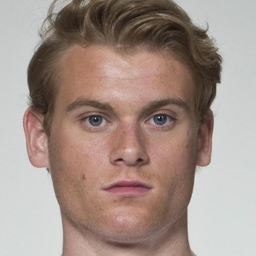
(a) Identity $a$

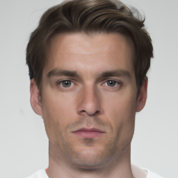
(b) Morphed image

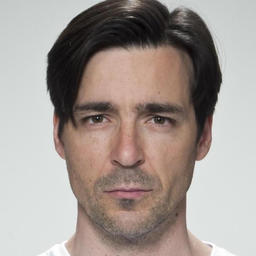
(c) Identity $b$

Figure 1: Example of a Diffusion-based morphing attack. Samples are from FRLL dataset.

Similar to the two classes of detection algorithms, there exist two broad classes of face morphing attacks: Landmark-based attacks and deep learning-based attacks. Landmark-based morphing attacks use local features to create the morphed image by warping and aligning the landmarks within each face then create a morphed face by pixel-wise compositing. Landmark-based attacks have been shown to be effective against FR systems [2]. In contrast, deep learning-based morphing attacks use a machine learning model to embed the original bona fide faces into a semantic representation which are then combined to produce a new representation that contains information from both identities. Recently, there has been an explosion of work exploring deep-learning based face morphing using generative models like Generative Adversarial Networks (GANs) [3, 4].

Recent work earlier this year by Blasingame et al. has pioneered the use of the Diffusion models for face morphing [5]. Other related work on Diffusion-based face morphing attacks[6] have followed the approach laid out by Blasingame et al. [5]. However, the design space of these Diffusion models is still mostly unexplored, leading to many questions in both implementation and methodology. In this work we explore three axes of Diffusion models, namely

1. Using faster sampling algorithms over the previous approach.

2. Exploring the “stochastic encoder” versus simply diffusing the image in accordance to the original Diffusion scheme.

3. Adding partial noise to the image instead of fully encoding into the stochastic latent space.

The effect of these design parameters is evaluated via visual inspection, the Fréchet Inception Distance (FID), and the Mated Morphed Presentation Match Rate (MMPMR).

II Related Work

Many varieties of face morphing attacks have been developed. While this work primarily examines the design space of the Diffusion-based approach [5], several other morphing attacks are considered for comparison purposes. For example, the FaceMorpher and OpenCV attacks are chosen as they commonly represent Landmark-based attacks [2, 1].

FaceMorpher is an open-source algorithm that uses the STASM landmark detector. Delaunay triangles are formed from the landmarks on the image, which are then warped and blended together. Areas outside the landmarks are averaged, typically introducing strong artefacts in the neck and hair regions of the image.

OpenCV is a face morphing algorithm based on the open-source OpenCV library with a 68-point annotator from the Dlib library. Delaunay triangles are formed from which landmarks are warped and blended. In contrast to the FaceMorpher algorithm, areas outside the landmarks do not consist of an averaged image, but rather additional Delaunay triangles. However, these morphs also exhibit notable artefacts outside the central region of the face.

Generative Adversarial Networks (GANs) are a common type of generative model used in face morphing attacks. GANs seek to learn the sampling process from some simple distribution to the data distribution via the generator network. An additional network called the discriminator is trained adversarially against the generator in a minimax game where the discriminator attempts to get better at distinguishing synthetic samples from genuine samples, while the generator tries to get better at deceiving the discriminator. For the face morphing attack, an encoding network which can embed images in the latent space such that the inversion has low distortion becomes necessary. Using this encoder, the latent codes for two identities are then averaged to produce a new latent code representing the morphed face which is then passed to the generator to create the morphed image. Notably, there exists a trade-off between the inversion distortion and editability of the latent embeddings. The StyleGAN2 [2] and MIPGAN-II [4] face morphing algorithms build upon the acclaimed StyleGAN2 architecture to create face morphs by averaging latent codes in the GAN latent space.

StyleGAN2 face morphs use the StyleGAN2 network which offers a host of improvements over the standard GAN implementation that enables the architecture to achieve state-of-the-art image quality when generating high resolution images. The StyleGAN2 model was pre-trained on the Flickr-Faces-HQ (FFHQ) dataset. The faces were then cropped to possess the same landmark alignment as in the FFHQ dataset. Images, $x_{a}$, $x_{b}$, are embedded by optimizing an initial latent code through stochastic gradient descent, minimizing the perceptual loss between the generated image and target image. Then once the embedded latent code, $z_{a}$, $z_{b}$, is found, a morphed latent code is created by linearly interpolating between the two, $z_{ab}=\textrm{lerp}(z_{a},z_{b};0.5)$. Lastly, the interpolated latent code is passed to the StyleGAN2 generator to get the morphed image.

MIPGAN-II proposes an extension on the face morphing approach from StyleGAN2 by adding an optimization procedure for the latent vector used in creating the morphed image [4]. The bona fide images are embedded into the latent space using the same StyleGAN2 optimization procedure. The latent code is initially constructed as a linear interpolation between these two embeddings. Then for $n$ epochs the latent code is optimized to minimize a combination of perceptual loss, identity loss, identity difference loss, and Multi-Scale Structural Similarity loss, finding a fully optimized latent $z_{n}$. The latent code $z_{n}$ is then passed to the StyleGAN2 generate to create the morphed image $x_{ab}$.

Algorithm 1 Face Morphing via Diffusion Autoencoders

$\mathbf{z}_{a}\leftarrow\mathcal{E}(\mathbf{x}_{0}^{(a)})$

$\mathbf{z}_{b}\leftarrow\mathcal{E}(\mathbf{x}_{0}^{(b)})$

$\mathbf{x}_{m}\leftarrow\frac{1}{2}(\mathbf{x}_{0}^{(a)}+\mathbf{x}_{0}^{(b)})$

$\mathbf{x}_{0}^{(a)}\leftarrow\mathbf{x}_{m}$

$\mathbf{x}_{0}^{(b)}\leftarrow\mathbf{x}_{m}$

for $i\leftarrow 1,2,\ldots N$ do

     $\mathbf{x}_{\tau_{i+1}}^{(a)}\leftarrow\lambda_{\tau_{i}}^{-}(\mathbf{x}_{\tau_{i}}^{(a)},\boldsymbol{\epsilon}_{\theta}(\mathbf{x}_{\tau_{i}}^{(a)},\mathbf{z}_{a},\tau_{i}))$

     $\mathbf{x}_{\tau_{i+1}}^{(b)}\leftarrow\lambda_{\tau_{i}}^{-}(\mathbf{x}_{\tau_{i}}^{(b)},\boldsymbol{\epsilon}_{\theta}(\mathbf{x}_{\tau_{i}}^{(b)},\mathbf{z}_{b},\tau_{i}))$

end for

$\mathbf{x}_{T}^{(ab)}\leftarrow\textrm{slerp}(\mathbf{x}_{T}^{(a)},\mathbf{x}_{T}^{(b)},0.5)$

$\mathbf{z}_{ab}\leftarrow\textrm{lerp}(\mathbf{z}_{a},\mathbf{z}_{b},0.5)$

for $i\leftarrow N,N-1,\ldots 1$ do

     $\mathbf{x}_{\tau_{i-1}}^{(ab)}\leftarrow\lambda_{\tau_{i}}(\mathbf{x}_{\tau_{i}}^{(ab)},\boldsymbol{\epsilon}_{\theta}(\mathbf{x}_{\tau_{i}}^{(ab)},\mathbf{z}_{ab},\tau_{i}))$

end for

return $\mathbf{x}_{0}^{(ab)}$

III Preliminaries

Diffusion models work by modeling the reverse trajectory of a stochastic differential equation (SDE) which perturbs the initial data distribution into isotropic Gaussian white noise over time. The image is degraded by slowly adding Gaussian noise in accordance to some noise schedule. This forward process $\{\mathbf{x}_{t}\}_{t\in[0,T]}$ is modeled as

$$q(\mathbf{x}_{t}\mid\mathbf{x}_{0})=\mathcal{N}(\mathbf{x}_{t}\mid\alpha_{t}\mathbf{x}_{0},\sigma_{t}^{2}\mathbf{I})$$ (1)

where $\alpha_{t}$ and $\sigma_{t}$ create the noise schedule for the Diffusion model, $\mathbf{x}_{0}$ is the real image, $\mathbf{x}_{t}$ denotes an image at timestep $t$ in the noise schedule, and $\mathbf{x}_{T}$ is the fully degraded image at terminal timestep $T$. Generally, the heart of the Diffusion model is a U-Net which predicts the added noise, or some other related quantity, that can be used by an SDE solver or similar algorithm, to calculate the reverse trajectory. The solver then uses the U-Net to move back from $t=T$ to $t=0$ with the goal of going from white noise, $\mathbf{x}_{T}\sim\mathcal{N}(\mathbf{0},\mathbf{I})$, to a sample from the data distribution, $\mathbf{x}_{0}\sim p(\mathbf{x}_{0})$.

The face morphing approach in [5] uses the Diffusion Autoencoder model proposed by Preechakul et al. [7] to create the face morphs. The Diffusion Autoencoder model consists of a conditioned noise prediction U-Net $\boldsymbol{\epsilon}_{\theta}:(\mathbf{x}_{t},\mathbf{z},t)\mapsto\hat{\epsilon}$ and encoder network $\mathcal{E}:\mathbf{x}_{0}\mapsto\mathbf{z}$ which learns the latent representation for an image [7]. This model uses the deterministic version of the Denoising Diffusion Implicit Model (DDIM) solver $\lambda_{\tau_{i}}:(\mathbf{x}_{\tau_{i}},\hat{\epsilon})\mapsto\mathbf{x}_{\tau_{i-1}}$ where $\{\tau_{i}\}_{i=1}^{N}\subseteq\{1,2,\ldots,T\}$ is the time schedule used for sampling with $N$ inference steps. Additionally, the deterministic DDIM solver is reversed to introduce the “stochastic encoder” $\lambda_{\tau_{i}}^{-}:(\mathbf{x}_{\tau_{i}},\hat{\epsilon})\mapsto\mathbf{x}_{\tau_{i+1}}$.

Let $\mathbf{x}_{0}^{(a)},\mathbf{x}_{0}^{(b)}$ denote face images of two bona fide subjects, $a$ and $b$. The face morphing strategy proposed in [5] is shown in Algorithm 1. At a high level this approach preforms an initial “pre-morph” by performing a pixel-wise average to obtain $\mathbf{x}_{m}$. This pre-morph is then encoded into the stochastic latent codes $\mathbf{x}_{T}^{(a)}$ and $\mathbf{x}_{T}^{(b)}$ by running the reverse DDIM solver. These stochastic latent codes are then morphed using spherical interpolation to give the morphed stochastic latent code $\mathbf{x}_{T}^{(ab)}$. The semantic latent codes are averaged to obtain $\mathbf{z}_{ab}$. These morphed latent codes are then used with the DDIM solver to generate the morphed imaged $\mathbf{x}_{0}^{(ab)}$. This approach is considered the “baseline” Diffusion-based face morphing approach for the purposes of this paper. The denoising U-Net used for the experiments in this paper was pre-trained on the FFHQ dataset at a $256\times 256$ resolution.

While this approach can achieve both state-of-the-art visual fidelity and high attack potency [5], the morphed images can look washed out or “blurry” in comparison to bona fide images, see Figure 1. This is most noticeable in the skin of the subject, often the morphs created via Diffusion-based model appear to be too “smooth”.

To assess the morphs generated by the face morphing algorithms, two main metrics are used: the Fréchet Inception Distance (FID) and Mated Morphed Presentation Match Rate (MMPMR). The FID metric is used to quantitatively assess the visual fidelity of the generated images as it has shown to correlate well with human assessment of fidelity [8]. The FID is a measure of distance between the generated and target distributions. As such, the lower the FID metric, the more similar the generated distribution is to the target distribution, which tends to correlate well with visual fidelity. The metric is defined as the Fréchet distance, or 2-Wasserstein metric between two Gaussian distributions, each representing the activations the deepest layer of an Inception v3 network induced by images from the generated and target distributions. The 2-Wasserstein metric between two probability measures $\mu,\nu$ with finite moments on $\mathbb{R}^{n}$ is defined as

$$W_{2}(\mu,\nu)=\bigg{(}\inf_{\pi\in\Pi(\mu,\nu)}\int_{\mathbb{R}^{n}\times\mathbb{R}^{n}}\|x-y\|_{2}^{2}\;\textrm{d}\pi(x,y)\bigg{)}^{\frac{1}{2}}$$ (2)

where $\Pi(\mu,\nu)$ is the set of all distributions with marginals $\mu$ and $\nu$.

The MMPMR metric is widely used as a measure of vulnerability of FR systems to face morphing attacks proposed by Scherhag et al. [9]. Two variants of the MMPMR metric for the scenario in which multiple bona fide images of an identity were used in morph process, excluding the images used in the creation of the morph, called the MinMax-MMPMR and ProdAvg-MMPMR. The MinMax-MMPMR metric is likely to increase the number of accepted morphs as the number of bona fide images per identity increases. Therefore, the ProdAvg-MMPMR is the specific MMPMR variant used to assess the vulnerability of FR systems. Any mention hereafter to MMPMR refers specifically to ProdAvg-MMPMR unless stated otherwise.

III-A Datasets

Different face morphing algorithms have created face morphs using images from the FRLL [10] and FRGC v2.0 [11] datasets, as they are commonly used for evaluation of face morphing attacks and have a large number of different identities [2, 3]. Notably, the FRLL dataset consists of many high quality close-up frontal images at a $1350\times 1350$ resolution with 189 facial landmarks. Morphs using OpenCV, FaceMorpher, and StyleGAN2 were created by Sarkar et al. [2] on the FRLL, FERET, and FRGC datasets. The MIPGAN-II morphs were created by Zhang et al. [4].

In order to create a morphed face, two component identities are needed. Naturally, if the two component identities are disparate, the resulting morph is likely to be very weak. To rectify this error and for evaluation purposes, the component identity pairs were selected by following the existing protocol used by Zhang et al. [4]. These pairings result in 534 unique morphs on FRLL and 274 on FRGC.

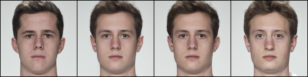
Figure 2: From left to right: identity $a$, morph generated with DDIM $(N=100)$, morph generated with DPM++ 2M $(N=20)$, identity $b$.

III-B Face Recognition Systems

Three publicly available FR systems are used to evaluate the face morphing attacks, specifically, the FaceNet, VGGFace2, and ArcFace models. These models are representative of recognition systems with state-of-the-art face verification performance [12, 13, 14]. For both models the last fully connected layer is used to provide a rich feature representation of the input image. Then for a presented face, its feature vector is compared with that of the feature vector belonging to the target face. If the distance between these two representations is sufficiently “small”, the presented face is then said to have the same identity as the target face. The VGGFace2 model improves upon acclaimed VGGFace by using an improved training dataset, also called VGGFace2. Following the introduction of Squeeze and Excitation Network, Cao et al. [12] presented the SENet architecture as the optimal choice when used with the VGGFace2 dataset. Google’s FaceNet model consists of an Inception-ResNet V1 architecture which is pre-trained on the VGGFace2 dataset [13]. A new state-of-the-art model, ArcFace [14], uses a novel loss function during training to improve the embeddings of faces. This loss function is known as Additive Angular Margin Loss or ArcFace Loss. The particular ArcFace model used for evaluation consists of a 100-layer Improved ResNet trained on the Glint360K dataset.

Additionally, the three FR systems use different pre-processing pipelines. Across all datasets the images and generated morphs are cropped as to be appropriate for passport photos; consequently, a face extractor is omitted from the verification pipeline. The FaceNet model resizes the image such that the short side of the image is 180 pixels long and then the image is cropped to a $160\times 160$ resolution. Lastly, the images are normalized to $[-1,1]$. The VGGFace2 model resizes the image such that the short side of the image is 256 pixels long and then crops the image to $224\times 224$ pixels. The mean RGB vector is subtracted from the cropped image to normalize the image. The ArcFace model resizes images such that the short side of the image is 112 pixels long which is then cropped to a $112\times 112$ resolution. The image is then normalized to have values in $[-1,1]$.

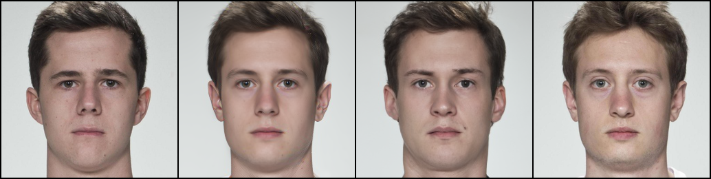
Figure 3: From left to right: identity $a$, morphed image using reverse DDIM solver, morphed image using white noise, identity $b$.

IV Faster Sampling Algorithms

The first axis of exploration is the sampling algorithm, or solver, used to sample the image from the initial white noise sample. One of the main problems with Diffusion models when compared to other generative models like GANs or Variational AutoEncoders (VAEs) is that it has significantly slower inference speed. In the original Diffusion formulation the diffusion process was realized discretely with $T=1000$ timesteps. Inference, therefore, required a 1000 iterations to generate an image. The DDIM solver improves this by using a strided sub-schedule to improve sampling speeds often around $N=100$. However, if one lowers the number of inference steps to say $N=20$, the DDIM solver is unlikely to produce good outputs as it often fails to converge. The work of Cheng et al. [15] introduces an efficient and fast ODE solver known as the “DPM++” solver which can sample the diffusion process. In particular, we use the 2nd-order variant denoted by “DPM++ 2M”. The DPM++ 2M solver is a high-order ODE solver with a convergence order guarantee, allowing high quality samples to be drawn in as little as 15 steps.

The connection between diffusion models, score-based modeling, and ODE solvers is provided as a summary. The diffusion process can be modeled continuously as an Itô SDE of the form

$$\textrm{d}\mathbf{x}_{t}=\mathbf{f}(\mathbf{x}_{t},t)\textrm{d}t+g(t)\textrm{d}\mathbf{w}_{t}$$ (3)

for a diffusion process $\{\mathbf{x}_{t}\}_{t\in[0,T]}$ where, $\mathbf{f}$ is a vector-valued function called the drift coefficient, $g$ is a scalar function called the diffusion coefficient, and $\mathbf{w}_{t}$ is the standard Wiener process. Now the reverse trajectory is given by the following reverse-time SDE

$$\textrm{d}\mathbf{x}_{t}=[\mathbf{f}(\mathbf{x}_{t},t)-g(t)^{2}\nabla_{\mathbf{x}}\log p_{t}(\mathbf{x}_{t})]\textrm{d}t+g(t)\textrm{d}\bar{\mathbf{w}}_{t}$$ (4)

where $p_{t}(\mathbf{x}_{t})$ is the marginal probability distribution at time $t$, $\bar{\mathbf{w}}_{t}$ is a standard Wiener process when time flows backwards from $T$ to $0$, and $\textrm{d}t$ is an infinitesimal negative timestep.

Unfortunately, the step size when discretizing SDEs is limited by the randomness of the Wiener process and a small number of inference steps, i.e., a large step size, can cause non-convergence of the sampler. Therefore, there exists an associated probability flow ODE which possesses the same marginal distribution at time $t$ as that of the SDE. The probability flow ODE associated with Equation 4 is

$$\frac{\textrm{d}\mathbf{x}_{t}}{\textrm{d}t}=\mathbf{f}(\mathbf{x}_{t},t)-\frac{1}{2}g(t)^{2}\nabla_{\mathbf{x}}\log p_{t}(\mathbf{x}_{t})$$ (5)

The quantity $\nabla_{\mathbf{x}}\log p_{t}(\mathbf{x}_{t})$ is known as the score function of the marginal distribution $p_{t}(\mathbf{x}_{t})$. Now generally, the score is learned through techniques like sliced score matching; however, in the case of diffusion models this can be greatly simplified. This problem reduces into simply predicting the noise that was added to the image at time $t$ is enough to approximate the score of the distribution. Therefore, with a noise prediction model, $\boldsymbol{\epsilon}_{\theta}(\mathbf{x}_{t},t)$, the probability flow ODE is parameterized as

$$\frac{\textrm{d}\mathbf{x}_{t}}{\textrm{d}t}=\mathbf{f}(\mathbf{x}_{t},t)+\frac{g(t)^{2}}{2\sigma_{t}}\boldsymbol{\epsilon}_{\theta}(\mathbf{x}_{t},t)$$ (6)

Then to generate a sample $\mathbf{x}_{0}$ from an initial latent sample $\mathbf{x}_{T}\sim\mathcal{N}(\mathbf{0},\mathbf{I})$, the probability flow ODE can be solved with some form of an ODE solver. The DPM++ 2M solver is a method for solving this ODE.

IV-A Evaluation

We implement the DPM++ 2M solver to work with the U-Net from the Diffusion Autoencoder model to allow for faster sampling. Following the procedure in Algorithm 1 the DDIM solver $\lambda_{t}$ is swapped out for the DPM++ 2M solver. To improve computation we used $N=20$ steps for the DPM++ 2M solver. With this significant reduction in sampling steps the FID was only impacted negatively in a slight manner with the FID still being far lower than other non-Diffusion based face morphing attacks, see Table II under the entry “Reverse DDIM, DPM++ 2M, N = 20”. In Figure 2 the morphed face generated by the DDIM solver is compared to the morphed face generated using the DPM++ 2M solver. Despite using far less inference steps, the difference is minor as reflected in the close FID values found in Table II.

In a similar vein the MMPMR metric took a slight decrease when switching over to the DPM++ 2M solver, see Table I, at the benefit of greatly improved inference speed. The drop was small but consistent across all datasets and FR systems. This could possibly be improved by using more steps, such as $N=50$, while still retaining time savings over the DDIM solver.

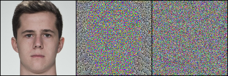
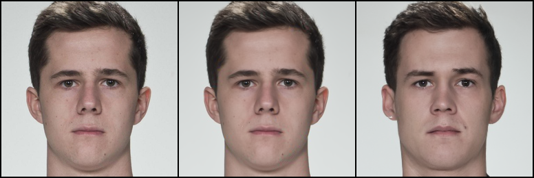
Figure 4: From top left to lower right: original image, reverse DDIM solver, diffused image, original image, sampled image from DDIM encode image, sampled image from diffused image.

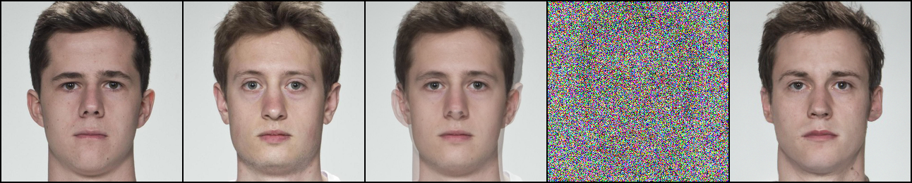
Figure 5: From left to right: identity $a$, identity $b$, pixel-wise averaged image, partially noised image $(\eta=0.6)$, final morphed image.

TABLE I: MMPMR at FMR = 0.1% across different morphing attacks. Higher is better.

	FRLL			FRGC
Morphing Attack	FaceNet	VGGFace2	ArcFace	FaceNet	VGGFace2	ArcFace
FaceMorpher	26.08	30.96	41.65	4.91	8.57	39.29
StyleGAN2	3.19	4.88	17.45	0.47	0.83	5.4
OpenCV	25.56	34.96	45.86	4.59	11.42	3.84
MIPGAN-II	15.38	21.39	51.59	3.5	7.48	32.68
Reverse DDIM, DDIM, N = 100	18.01	29.46	84.05	3.83	7.81	45.89
Reverse DDIM, DPM++ 2M, N = 20	17.07	28.89	82.74	3.68	7.75	38.68
Noise = 1.0, DPM++ 2M, N = 20	2.63	1.5	3.19	0.66	0.75	2.81
Noise = 0.6, DPM++ 2M, N = 50	3	3.75	8.63	0.78	1.56	6.24

V Reverse DDIM Solver

The second axis of exploration is the reverse DDIM solver, $\lambda_{t}^{-}$ used to encode the original image $\mathbf{x}_{0}$ into its stochastic latent code $\mathbf{x}_{T}$. In the Diffusion framework $\mathbf{x}_{T}$ is generally sampled from $\mathcal{N}(\mathbf{0},\mathbf{I})$ as the terminal distribution. The forward diffusion process described in Equation 1 can be calculated in one step with

$$\mathbf{x}_{t}=\sqrt{\bar{\alpha}_{t}}\mathbf{x}_{0}+\sqrt{1-\bar{\alpha}_{t}}\epsilon$$ (7)

where $\epsilon\sim\mathcal{N}(\mathbf{0},\mathbf{I})$ and $\bar{\alpha}_{t}=\sum_{s=1}^{t}\alpha_{s}$ for discretized diffusion parameters $\{\alpha_{t}\}$ with the usual diffusion parameter schedule $\mathbf{x}_{T}\sim\mathcal{N}(\mathbf{0},\mathbf{I})$. However, the reverse DDIM solver does not encode $p(\mathbf{x}_{0})$ into $p(\mathbf{x}_{T})$, but rather some other distribution.

In Figure 4 the original image is encoded by the reversed DDIM solver to obtain the stochastic latent code and is also encoded following the process in Equation 1 to obtain $\mathbf{x}_{T}$.

The reverse DDIM solver used $N=250$ steps and the forward DDIM solver used $N=100$ steps. While the image encoded following the Diffusion process appears to be sampled from isotropic Gaussian noise as one would expect, the image encoded using the reverse DDIM solver is not drawn from the Gaussian distribution. Rather this latent noise contains “stochastic” information of the subject rather than be truly white noise. When paired with the DDIM solver the reconstructed image, bottom middle image in Figure 4, is a close reconstruction, albeit with some high frequency details missing, resulting in a smooth appearance. In contrast, the image which was diffused to white noise and then run through the DDIM solver retains some high level characteristics with the original image, due to the semantic latent code, but with some stochastic details changed. The morphed image generated from the stochastic latent code appears to be more “smoothed” out than the image generated from white noise.

Figure 3 compares the differences in face morphing when using the combined stochastic latent code found from reverse DDIM solver and starting from white noise. The later approach starting the DDIM sampling from white noise allows the semantic latent code $\mathbf{z}_{ab}$ to guide the morph generation with small stochastic details to be controlled by $\mathbf{x}_{T}\sim\mathcal{N}(\mathbf{0},\mathbf{I})$. Matching the observation from autoencoding test in Figure 4, the morphed image that started from white noise has more high frequency detail and in generally appears more realistic. This is accompanied with a greatly decreased FID score, see Table II under “Noise = 1.0, DPM++ 2M, N = 20”. Ignore the “stochastic encoder” of the Diffusion Autoencoder model not only greatly improves inference speed, $N=250$ U-Net steps for the forward process versus simply adding white noise to the image like in the traditional forward process, but it also improves visual fidelity. In our experience using the DPM++ 2M solver and random stochastic latent $\mathbf{x}_{T}$ improves inference speed of upwards of 90%.

Unfortunately, unlike the significant improvements in visual fidelity, the MMPMR plummeted precipitously, see Table I. This caused the MMPMR to drop to the lowest of any of the Diffusion-based morphs. It seems likely that the FR system favors the averaged, “blurry” looking features of the reference Diffusion-based morphs over more realistic images produced by this method, which remove certain stochastic attributes present from the original image.

TABLE II: FID across different morphing attacks. Lower is better.

Morph	FRLL	FRGC
StyleGAN2	49.01	95.30
FaceMorpher	94.06	100.53
OpenCV	88.44	113.02
MIPGAN-II	66.78	116.90
Reverse DDIM, DDIM, N = 100	42.25	74.75
Reverse DDIM, DPM++ 2M, N = 20	46.64	82.32
Noise = 1.0, DPM++ 2M, N = 20	27.01	68.27
Noise = 0.6, DPM++ 2M, N = 50	26.66	60.81

VI Partial Sampling

The third axis of exploration is how much noise is added to the original images during the forward diffusion process. That is, instead of running the DDIM solver through the complete time schedule $\{\tau_{i}\}_{i=1}^{N}$, one could use a sub-schedule $\{\tau_{i}\}_{i=1}^{M}$, $M<N$. In essence this functions as a control on how much the Diffusion model alters the image with $M\to 0$ leading to no changes to the original image. Instead of explicitly choosing $M$, a noise level $\eta\in[0,1]$ is chosen, which represents the amount of noise added to the image with $M=\lfloor\eta N\rfloor$.

The diffusion process can be thought of as slowly removing information away from the original image until no information remains. Now by halting the diffusion process part way through we only remove partial information, not everything. In reality we mostly remove high frequency information, as low frequency information is some of the last to disappear. This means that for face morphing the parameter $\eta=0.6$ controls how much information we remove from our original image before adding new information back in through our latent code. This inspires the following process wherein a low effort morph $\mathbf{x}_{m}=\frac{1}{2}(\mathbf{x}_{0}^{(a)}+\mathbf{x}_{0}^{(b)})$ has noise added according to

$$\mathbf{x}_{\tau_{M}}=\sqrt{\bar{\alpha}_{\tau_{M}}}\mathbf{x}_{m}+\sqrt{1-\bar{\alpha}_{M}}\epsilon$$ (8)

with some Gaussian noise $\epsilon$. This obscures a lot of the strange artefacts that would occur in a simple pixel-wise average morph, but retaining some information from the original identities. The DPM++ 2M solver is then run from backwards through the time schedule $\{\tau_{i}\}_{i=1}^{M}$ eventually yielding the morphed image $\mathbf{x}_{0}^{(ab)}$.

Figure 5 provides a snapshot of the different phases in this face morphing pipeline, from the original two bona fide images, to the pixel-wise averaged image, to the noised image, and to the final morphed image. Notably, the morphed image seems to have higher visual fidelity than the morphed images from Figures 4 and 3 possessing sharper high frequency details and natural looking physical features. To further this natural observation the FID of this approach, see the entry “Noise = 0.6, DPM++ 2M, N = 50” has the lowest FID scores of any of the morphing algorithms studied.

Yet again, the excellent FID scores are contrasted with poor MMPMR scores, see Table I. However, the partial sampling approach does have a slight edge over the the fully diffusing the image in MMPMR. Moreover, it does so while retaining a better FID score than the prior approach. Additionally, because the approach only partial samples it takes even less computation time than sampling from fully diffused image, again improving inference speed.

VII Summary of Findings

In general by observing Tables II and I techniques which improved the visual fidelity seemed to decrease the MMPMR. It’s possible that a more “averaged” face with prominent artefacts, like OpenCV and FaceMorpher, is ideal in tricking a FR system; whereas a morphed image which increased visual fidelity might lose its effectiveness. That said, a morphed image would need a baseline level of visual fidelity if a human agent is involved. Moreover, it is trivial to train a detector to notice such prominent artefacts [1, 5].

The poor MMPMR results after abandoning the stochastic latent code seems to imply that the initial theory that the semantic latent code contains all high-level semantic information and the stochastic latent code contains all stochastic information offered by the Diffusion Autoencoder authors is not fully correct. For the semantic information should be what triggers an accept or reject in the FR system. However, these FR systems seem very sensitive to the stochastic latent code in the Diffusion Autoencoders.

VIII Conclusion

We explore the design space of Diffusion Autoencoders within the context of face morphing attacks. We discover several techniques which impact the visual fidelity and the effectiveness of the morphed images. We were able to greatly accelerate the speed at which face morphs are created using Diffusion Autoencoders, enabling the creation of large scale face morphing datasets. In our experimentation we were able to greatly increase the visual fidelity of face morphs created using Diffusion Autoencoders. Unfortunately, the increase in visual fidelity seems to accompany a decrease in the effectiveness of the morphing attack in fooling an FR system. This leads to an interesting question on the relationship between the visual fidelity of the morphed image and the effectiveness of the morphed image.

References

- [1] Z. Blasingame and C. Liu, “Leveraging adversarial learning for the detection of morphing attacks,” 2021 IEEE International Joint Conference on Biometrics (IJCB), pp. 1–8, 2021.
- [2] E. Sarkar, P. Korshunov, L. Colbois, and S. Marcel, “Vulnerability analysis of face morphing attacks from landmarks and generative adversarial networks,” ArXiv, vol. abs/2012.05344, 2020.
- [3] ——, “Are gan-based morphs threatening face recognition?” in ICASSP 2022 - 2022 IEEE International Conference on Acoustics, Speech and Signal Processing (ICASSP), 2022, pp. 2959–2963.
- [4] H. Zhang, S. Venkatesh, R. Ramachandra, K. Raja, N. Damer, and C. Busch, “Mipgan—generating strong and high quality morphing attacks using identity prior driven gan,” IEEE Transactions on Biometrics, Behavior, and Identity Science, vol. 3, no. 3, pp. 365–383, 2021.
- [5] Z. Blasingame and C. Liu, “Leveraging diffusion for strong and high quality face morphing attacks,” 2023.
- [6] N. Damer, M. Fang, P. Siebke, J. N. Kolf, M. Huber, and F. Boutros, “Mordiff: Recognition vulnerability and attack detectability of face morphing attacks created by diffusion autoencoders,” 2023. [Online]. Available: https://publica.fraunhofer.de/handle/publica/444950
- [7] K. Preechakul, N. Chatthee, S. Wizadwongsa, and S. Suwajanakorn, “Diffusion autoencoders: Toward a meaningful and decodable representation,” in Proceedings of the IEEE/CVF Conference on Computer Vision and Pattern Recognition (CVPR), June 2022, pp. 10 619–10 629.
- [8] M. Lucic, K. Kurach, M. Michalski, O. Bousquet, and S. Gelly, “Are gans created equal? a large-scale study,” in Proceedings of the 32nd International Conference on Neural Information Processing Systems, ser. NIPS’18. Red Hook, NY, USA: Curran Associates Inc., 2018, p. 698–707.
- [9] U. Scherhag, A. Nautsch, C. Rathgeb, M. Gomez-Barrero, R. N. J. Veldhuis, L. Spreeuwers, M. Schils, D. Maltoni, P. Grother, S. Marcel, R. Breithaupt, R. Ramachandra, and C. Busch, “Biometric systems under morphing attacks: Assessment of morphing techniques and vulnerability reporting,” in 2017 International Conference of the Biometrics Special Interest Group (BIOSIG), 2017, pp. 1–7.
- [10] L. DeBruine and B. Jones, “Face research lab london set.”
- [11] P. Phillips, P. Flynn, T. Scruggs, K. Bowyer, J. Chang, K. Hoffman, J. Marques, J. Min, and W. Worek, “Overview of the face recognition grand challenge,” in 2005 IEEE Computer Society Conference on Computer Vision and Pattern Recognition (CVPR’05), vol. 1, 2005, pp. 947–954 vol. 1.
- [12] Q. Cao, L. Shen, W. Xie, O. M. Parkhi, and A. Zisserman, “Vggface2: A dataset for recognising faces across pose and age,” in 2018 13th IEEE International Conference on Automatic Face & Gesture Recognition (FG 2018), 2018, pp. 67–74.
- [13] F. Schroff, D. Kalenichenko, and J. Philbin, “Facenet: A unified embedding for face recognition and clustering,” in 2015 IEEE Conference on Computer Vision and Pattern Recognition (CVPR), 2015, pp. 815–823.
- [14] J. Deng, J. Guo, N. Xue, and S. Zafeiriou, “Arcface: Additive angular margin loss for deep face recognition,” in Proceedings of the IEEE Conference on Computer Vision and Pattern Recognition, 2019, pp. 4690–4699.
- [15] C. Lu, Y. Zhou, F. Bao, J. Chen, C. Li, and J. Zhu, “Dpm-solver++: Fast solver for guided sampling of diffusion probabilistic models,” 2023.