Extremum seeking in the presence of large delays via time-delay approach to averaging

Abstract

In this paper, we study gradient-based classical extremum seeking (ES) for uncertain n-dimensional (nD) static quadratic maps in the presence of known large constant distinct input delays and large output constant delay with a small time-varying uncertainty. This uncertainty may appear due to network-based measurements. We present a quantitative analysis via a time-delay approach to averaging. We assume that the Hessian has a nominal known part and norm-bounded uncertainty, the extremum point belongs to a known box, whereas the extremum value to a known interval. By using the orthogonal transformation, we first transform the original static quadratic map into a new one with the Hessian containing a nominal diagonal part. We apply further a time-delay transformation to the resulting ES system and arrive at a time-delay system, which is a perturbation of a linear time-delay system with constant coefficients. Given large delays, we choose appropriate gains to guarantee stability of this linear system. To find a lower bound on the dither frequency for practical stability, we employ variation of constants formula and exploit the delay-dependent positivity of the fundamental solutions of the linear system with their tight exponential bounds. Sampled-data ES in the presence of large distinct input delays is also presented. Explicit conditions in terms of simple scalar inequalities depending on tuning parameters and delay bounds are established to guarantee the practical stability of the ES control systems. We show that given any large delays and initial box, by choosing appropriate gains we can achieve practical stability for fast enough dithers and small enough uncertainties.

1 Introduction

ES is a model-free, real-time on-line adaptive optimization control method. In 2000, Krstic and Wang gave the first rigorous stability analysis for an ES system by using averaging and singular perturbations in [9], which laid a theoretical foundation for the development of ES. Subsequently, a great amount of theoretical and applied studies on ES are emerging, see e.g. non-local ES control in [20], Newton-based ES in [7, 13], ES via Lie bracket approximation in [3, 10], stochastic ES in [11] and ES control for wind farm power maximization in [4].

The time-delay phenomenon often exists in applications of ES, due to time needed to measuring and processing of the data ([12, 15, 16]). The existence of time-delay can cause performance deterioration and even instability of the ES control system. To address the challenges of delays in extremum seeking, Oliveira et al. in [15] provided classical predictors for delayed gradient and Newton-based methods. This work was later extended to single-variable ES with uncertain constant delay in [17], and with time-varying delay in [14, 18]. Recently, Malisoff et al. in [12] reconsidered the multi-variable ES for static maps with arbitrarily long time constant delays by using a one-stage sequential predictor, which can avoid the interference of the integral term appeared in [15]. However, these methods provide only qualitative analysis employing the classical averaging theory in infinite dimensions (see [8]), and cannot suggest quantitative bounds on the dither frequency that preserve the stability.

Recently, a new constructive time-delay approach to the continuous-time averaging was presented in [6] with efficient and quantitative bounds on the small parameter that ensures the stability. The time-delay approach to averaging was successfully applied for the quantitative stability analysis of continuous-time ES algorithms in [24] and sampled-data ES algorithms in [26] for static quadratic maps by constructing appropriate Lyapunov-Krasovskii (L-K) functionals. However, the analysis via L-K method is complicated and the results may be conservative. In our recent paper [22] we suggested a robust time-delay approach to ES, where we presented the resulting time-delay model as a non-delayed one with disturbances and further employed a variation of constants formula. The latter can greatly simplify the stability analysis via L-K method, simplify the conditions and reduce conservatism.

In this paper, we consider the multi-variable ES of uncertain static quadratic maps with known large constant distinct input delays and large output constant delay with a small uncertain fast-varying delay (without constraints on the delay derivative). Note that each individual input channel may induce a different delay (see [2]), whereas the delay uncertainty may appear due to network-based measurements (see [5]). We first transform the original static quadratic map into a new one with the Hessian containing a nominal diagonal part, and then apply a time-delay approach to the resulting ES system to get a time-delay system, which is a perturbation of a linear time-delay system with constant coefficients. Finally, we use the variation of constants formula to quantitatively analyze the practical stability of the retarded systems (and thus of the original ES systems). In the stability analysis, we exploit positivity of the fundamental solution that corresponds to the nominal time-delay system to obtain tighter bounds. Moreover, the sampled-data ES in the presence of large distinct input delays is also presented. Explicit conditions in terms of simple inequalities are established to guarantee the practical stability of the ES control systems. Through the solution of the constructed inequalities, we find upper bounds on the dither period that ensures the practical stability, and also provide quantitative ultimate bound (UB) on estimation error. We show that given any large delays and initial box, by choosing appropriate gains we can achieve practical stability for fast enough dithers and small enough uncertainties. Note that if the Hessian is completely unknown, quantitative results seem to be not possible, since the Hessian is used in ES algorithm to provide an estimate of the gradient.

We summarize the contribution as follows: 1) For the first time, quantitative conditions are presented for ES of partly known static quadratic maps in the presence of large input and output delays, where uncertain fast-varying measurement delay (that may appear due to e.g. network-based measurements) and distinct input delays are taken into account. Note that in the existing qualitative results [12, 15] the case of distinct delays in the map (and not in the inputs) is considered, whereas in [14, 18] the delays are known and slowly-varying (with the delay derivative less than one). 2) Differently from the existing ES results via the time-delay approach [22, 24, 25, 26], in the present paper we suggest to start with diagonalization of the nominal part of the quadratic map and further exploit positivity of the fundamental solutions of the time-delay equations with their tight bounds. This leads to simplified and less conservative conditions. 3) For the first time we present sampled-data implementation of ES control of nD quadratic static map in the presence of large distinct input delays. Note that in [25, 26], one and two input variables with a single delay of the order of the small parameter were considered.

The paper’s rest organization is as follows: In Section 2, we present some notation and preliminaries. In Section 3 and Section 4, we apply the time-delay approach to gradient-based classical ES and sampled-data ES, respectively. The latter sections contain two parts: the theoretical results and examples with simulations. Section 5 concludes this paper.

2 Notation and Preliminaries

Notation: The notation used in this paper is fairly standard. The notations $\mathbf{Z}_{+}$ and $\mathbf{N}$ refer to the set of nonnegative integers and positive integers, respectively. The notation $P>0$ ($<0$) for $P\in\mathbf{R}^{n\times n}$ means that $P$ is symmetric and positive (negative) definite. $I_{n}$ is the $n\times n$ identity matrix. The notations $\left|\cdot\right|$ and $\left\|\cdot\right\|$ refer to the Euclidean vector norm and the induced matrix $2$ norm, respectively.

We will employ the variation of constants formula for delay differential equations and some properties of the corresponding fundamental solutions as in the following lemma, these results are brought from [1] (see Lemma 2.1, Theorem 2.7 and Corollary 2.14).

Lemma 1.

Consider the following scalar delay differential equation:

$$\left.\dot{x}(t)+ax(t-g(t))=f(t),\text{ }t\geq t_{0}\right.$$ (1)

with the initial value

$$x(t)=\varphi(t),\text{ }t<t_{0},\text{ }x(t_{0})=x_{0},$$ (2)

where $g:[t_{0},\infty)\rightarrow\mathbf{R}$ is a Lebesgue measurable function, $f:[t_{0},\infty)\rightarrow\mathbf{R}$ is a Lebesgue measurable locally essentially bounded function and $\varphi:(-\infty,t_{0})\rightarrow\mathbf{R}$ is a piecewise continuous and bounded function. Then there exists one and only one solution for (1)-(2) as in the following form

$$\left.\begin{array}[c]{l}x(t)=X(t,t_{0})x_{0}+{\textstyle\int\nolimits_{t_{0}}^{t}}X(t,s)f(s)\mathrm{d}s\\ \text{ \ \ \ \ \ \ \ \ }-{\textstyle\int\nolimits_{t_{0}}^{t}}X(t,s)a\varphi(s-g(s))\mathrm{d}s,\end{array}\right.$$ (3)

where $\varphi(s-g(s))=0$ if $s-g(s)>t_{0}\mathbf{,}$ and the fundamental solution $X(t,s)$ is the solution of

$$\left.\begin{array}[c]{l}\dot{x}(t)+ax(t-g(t))=0,\text{ }t\geq s,\\ x(t)=0,\text{ }t<s,\text{ }x(s)=1.\end{array}\right.$$

Particularly, let $a>0,$ $0\leq g(t)\leq L,$ $t\geq t_{0}$ and

$$\left.LA\leq\frac{1}{\mathrm{e}},\text{ }t\geq t_{0}.\right.$$

Then for $t>s\geq t_{0},$

$$\left.0<X(t,s)\leq\left\{\begin{array}[c]{ll}1,&s\leq t\leq s+L,\\ \mathrm{e}^{-a(t-s-L)},&t\geq s+L.\end{array}\right.\right.$$

3 ES with Large Distinct Delays

3.1 Multi-variable static map

Consider multi-variable static maps with measurement delay given by:

$$\left.\begin{array}[c]{l}y(t)=Q(\theta(t-D_{\mathrm{out}}(t)))\\ \text{ \ \ \ \ }=Q^{\ast}+\frac{1}{2}[\theta(t-D_{\mathrm{out}}(t))-\theta^{\ast}]^{\mathrm{T}}\\ \text{ \ \ \ \ \ \ \ }\times H[\theta(t-D_{\mathrm{out}}(t))-\theta^{\ast}],\end{array}\right.$$ (4)

where $y(t)\in\mathbf{R}$ is the measurable output, $\theta(t)\in\mathbf{R}^{n}$ is the vector input, $Q^{\ast}\in\mathbf{R}$ and $\theta^{\ast}\in\mathbf{R}^{n}$ are constants, $H=H^{\mathrm{T}}$ is the Hessian matrix which is either positive definite or negative definite, and $D_{\mathrm{out}}(t)=D+\Delta D(t).$ Here $D>0$ is a large and known constant and $\Delta D(t)$ is a small time-varying uncertainty satisfying $\left|\Delta D(t)\right|\leq\rho$, where $\rho\geq 0$ is a small known constant. The fast-varying (without any constraints on the delay derivative) delay uncertainty may appear due to sampling of the measurement data or network-based measurements (see [5], Chapter 7). Moreover, we also consider the ES in the presence of distinct known constant input delays $D_{i}^{\mathrm{in}}>0$ $(i=1,\ldots,n)$. For future use, we denote for $i=1,\ldots,n\mathbf{,}$

$$\left.\begin{array}[c]{l}D_{i}(t)=D_{i}^{\mathrm{in}}+D_{\mathrm{out}}(t),\text{ }\bar{D}_{i}=D_{i}^{\mathrm{in}}+D,\\ D_{i\mathrm{M}}=D_{i}^{\mathrm{in}}+D+\rho,\text{ }D_{\text{{M}}}=\max_{i=1,\ldots,n}D_{i\mathrm{M}}.\end{array}\right.$$ (5)

We assume that the nominal values of delays $\bar{D}_{i}$ are commensurable:

A1. $\bar{D}_{i}/\bar{D}_{j}$ $(\forall i,j=1,\ldots,n)$ are rational, meaning that for some $m_{i}\in\mathbf{N}$ $(i=1,\ldots,n)$ the following holds:

$$m_{i}\bar{D}_{j}=m_{j}\bar{D}_{i},\text{ }\forall i,j=1,\ldots,n\mathbf{.}$$ (6)

In the design, we will choose the corresponding $m_{i}$ $(i=1,\ldots,n)$ as small as possible.

Without loss of generality, we assume that the quadratic map (4) has a minimum value $y(t)=Q^{\ast}$ at $\theta=\theta^{\ast}$, and then $H>0$. In order to derive efficient quantitative conditions, we further assume that:

A2. The extremum point $\theta^{\ast}=[\theta_{1}^{\ast},\ldots,\theta_{n}^{\ast}]^{\mathrm{T}}$ to be sought is uncertain from some known box $\theta_{i}^{\ast}\in[\underline{\theta}_{i}^{\ast},\bar{\theta}_{i}^{\ast}]$ with $\left|\bar{\theta}_{i}^{\ast}-\underline{\theta}_{i}^{\ast}\right|=\sigma_{0i},$ $i=1,\ldots,n.$

A3. The extremum value $Q^{\ast}$ is unknown, but it is subject to $\left|Q^{\ast}\right|\leq Q_{\mathrm{M}}^{\ast}$ with $Q_{\mathrm{M}}^{\ast}$ being known.

A4. The Hessian $H$ is uncertain and subject to $H=\bar{H}+\Delta H$ with $\bar{H}>0$ being known nominal part of $H$ and $\left\|\Delta H\right\|\leq\kappa.$ Here $\kappa\geq 0$ is a known scalar.

Remark 1.

In classical ES, the Hessian $H$, the extremum value $Q^{\ast}$ and the extremum point $\theta^{\ast}$ in (4) are assumed to be unknown, where tuning parameters may be found from simulations only. Here we study a ”grey box” model with Assumptions A2-A4 and provide a quantitative analysis. There is a tradeoff between the quantitative analysis with the plant information and the qualitative analysis without the model knowledge.

Since $\bar{H}>0$ is known, we can find an orthogonal matrix $U\in\mathbf{R}^{n\times n}$ (obviously, $\left\|U\right\|=1$) such that

$$\left.U\bar{H}U^{\mathrm{T}}=\mathrm{diag}\{\bar{h}_{1},\ldots,\bar{h}_{n}\}>0.\right.$$ (7)

Let

$$\left.\begin{array}[c]{l}\mathcal{H}=UHU^{\mathrm{T}},\text{ }\mathcal{\bar{H}}=U\bar{H}U^{\mathrm{T}},\text{ }\Delta\mathcal{H}=U\Delta HU^{\mathrm{T}},\\ \vartheta(t)=U\theta(t),\text{ }\vartheta^{\ast}=U\theta^{\ast}.\end{array}\right.$$ (8)

Then the cost function (4) can be rewritten as

$$\left.\begin{array}[c]{l}y(t)=Q(U^{\mathrm{T}}\vartheta(t-D_{\mathrm{out}}(t)))\\ \text{ \ \ \ \ }=Q^{\ast}+\frac{1}{2}[\vartheta(t-D_{\mathrm{out}}(t))-\vartheta^{\ast}]^{\mathrm{T}}\\ \text{ \ \ \ \ \ \ \ }\times\mathcal{H}[\vartheta(t-D_{\mathrm{out}}(t))-\vartheta^{\ast}]\end{array}\right.$$ (9)

with the diagonal nominal part $\mathcal{\bar{H}}$ of the Hessian $\mathcal{H}$:

$$\mathcal{H}=\mathcal{\bar{H}}+\Delta\mathcal{H},\text{ }\mathcal{\bar{H}}=\mathrm{diag}\{\bar{h}_{1},\bar{h}_{2},\ldots,\bar{h}_{n}\}.$$ (10)

Now define the real-time estimates $\hat{\theta}(t)$ and $\hat{\vartheta}(t)$ of $\theta^{\ast}$ and $\vartheta^{\ast}$, respectively, with the estimation errors:

$$\left.\tilde{\theta}(t)=\hat{\theta}(t)-\theta^{\ast},\text{ }\tilde{\vartheta}(t)=\hat{\vartheta}(t)-\vartheta^{\ast}.\right.$$ (11)

Design $\hat{\theta}(t)=U^{\mathrm{T}}\hat{\vartheta}(t),$ then from (8) and (11), we have $\tilde{\theta}(t)=U^{\mathrm{T}}\tilde{\vartheta}(t)$, which implies $|\tilde{\theta}(t)|=|\tilde{\vartheta}(t)|.$ Therefore, it is sufficient to find bounds on $\tilde{\vartheta}(t)$.

In the ES, we use the dither signals $S(t)$ and $M(t)$ as:

$$\left.\begin{array}[c]{l}S(t)=[S_{1}(t),\ldots,S_{n}(t)]^{\mathrm{T}},S_{i}(t)=a_{i}\sin(\omega_{i}t),\\ M(t)=[M_{1}(t),\ldots,M_{n}(t)]^{\mathrm{T}},M_{i}(t)=\frac{2}{a_{i}}\sin(\omega_{i}t),\end{array}\right.$$ (12)

where the frequencies $\omega_{i}\neq\omega_{j},i\neq j$ are non-zero, $\omega_{i}/\omega_{j}$ are rational and $a_{i}$ are non-zero real numbers. Choose the adaptation gain

$$\left.K=\mathrm{diag}\{k_{1},\ldots,k_{n}\},\text{ }k_{i}<0\right.$$ (13)

such that $K\mathcal{\bar{H}}$ is Hurwitz. Let the control law be in the form:

$$\left.\begin{array}[c]{l}u_{i}(t)=k_{i}M_{i}(t+D_{i}^{\mathrm{in}})y(t),\\ \vartheta_{i}(t)=\hat{\vartheta}_{i}(t)+S_{i}(t),\text{ }t\geq D_{\text{{M}}}.\end{array}\right.$$ (14)

Then the gradient-based classical ES algorithm in the presence of distinct input delays is governed by ($i=1,\ldots,n$)

$$\left.\dot{\hat{\vartheta}}_{i}(t)=\left\{\begin{array}[c]{lc}0,&t\in[0,D_{\text{{M}}}),\\ u_{i}(t-D_{i}^{\mathrm{in}}),&t\in[D_{\text{{M}}},\infty),\end{array}\right.\right.$$ (15)

Control law (15) means that we wait and start all control actions $u_{i}(t-D_{i}^{\mathrm{in}})$ $(i=1,\ldots,n)$ at the same time $t=D_{\text{{M}}}$, which simplifies the stability analysis.

By (9), (11) and (12)-(15), the estimation error is governed by ($i=1,\ldots,n$)

$$\left.\begin{array}[c]{l}\dot{\tilde{\vartheta}}_{i}(t)=k_{i}M_{i}(t)Q^{\ast}+\frac{1}{2}k_{i}M_{i}(t)\\ \text{ \ \ }\times[S(t-D_{i}(t))+\tilde{\vartheta}(t-D_{i}(t))]^{\mathrm{T}}\mathcal{H}\\ \text{ \ \ }\times[S(t-D_{i}(t))+\tilde{\vartheta}(t-D_{i}(t))],\text{ }t\geq D_{\text{{M}}}\mathbf{,}\\ \tilde{\vartheta}_{i}(t)=\tilde{\vartheta}_{i}(D_{\text{{M}}}),\text{ }t\in[0,D_{\text{{M}}}].\end{array}\right.$$ (16)

Remark 2.

It is seen from (16) that in each subsystem, the delay $D_{i}(t)$ keeps the same value for the whole state $\tilde{\vartheta}$, which is different from [12, 15] with a simplified form $\tilde{\vartheta}\left(t-D\right):=[\tilde{\vartheta}_{1}\left(t-D_{1}\right),\ldots,\tilde{\vartheta}_{n}\left(t-D_{n}\right)]^{\mathrm{T}}.$ The latter form corresponds to an abstract map (9) with $\vartheta(t-D_{\mathrm{out}}(t))$ changed by $\vartheta(t-D_{\mathrm{out}}(t))=[\vartheta_{1}(t-D_{1}),\ldots,\vartheta_{n}(t-D_{n})]^{\mathrm{T}}$ studied in these papers, but not to the case of distinct input delays in the ES algorithm. Note that in this simplified case, one do not need assumption A4 on commensurable delays $\bar{D}_{i}$ as well as on the special choice of dither frequencies (as defined by (17) of the following Lemma 2). The time-varying delays case considered here is also more general than the constant delay case in [12, 15].

Remark 3.

Denote $U=[b_{ij}]_{n\times n}$. Since $\theta(t)=U^{\mathrm{T}}\vartheta(t)$ and $\hat{\theta}(t)=U^{\mathrm{T}}\hat{\vartheta}(t),$ then from (14) and (15) it is easy to present the gradient-based classical ES algorithm for the original ES problem as follows ($i=1,\ldots,n$):

$$\left.\dot{\hat{\theta}}_{i}(t)=\left\{\begin{array}[c]{lc}0,&t\in[0,D_{\text{{M}}}),\\ {\textstyle\sum\limits_{j=1}^{n}}b_{ji}u_{j}(t-D_{j}^{\mathrm{in}}),&t\in[D_{\text{{M}}},\infty),\end{array}\right.\right.$$

with

$$\left.\begin{array}[c]{l}u_{i}(t)=k_{i}M_{i}(t+D_{i}^{\mathrm{in}})y(t),\\ \theta_{i}(t)=\hat{\theta}_{i}(t)+{\textstyle\sum\limits_{j=1}^{n}}b_{ji}S_{j}(t),\text{ }t\geq D_{\text{{M}}}.\end{array}\right.$$

By using this algorithm and noting that $\tilde{\theta}(t)=U^{\mathrm{T}}\tilde{\vartheta}(t),$ we can obtain part (ii) in Theorem 1 below. The corresponding analysis is also suitable for the sampled-data ES case in Section 4.

To choose appropriate dither frequencies, we will employ the following lemma, which is proved in Appendix:

Lemma 2.

Under A1, consider the following positive numbers (frequencies):

$$\left.\omega_{i}=\frac{q\cdot 2\pi im_{j}}{\bar{D}_{j}},\text{ }q\in\mathbf{N},\text{ }\forall i,j=1,\ldots,n\mathbf{.}\right.$$ (17)

Then the following relations hold:

$$\left.\sin(\omega_{i}(t-\bar{D}_{j}))=\sin(\omega_{i}t),\text{ }\forall i,j=1,\ldots,n\mathbf{.}\right.$$ (18)

Based on Lemma 2, we assume that:

A5. The frequencies are chosen according to (17) with some $q\in\mathbf{N}$.

Due to (17), the frequencies $\omega_{i}=\omega_{i,q}$ $(i=1,\ldots,n)$ can be always chosen larger than any $\omega^{\ast}>0$. Using Lemma 2, we have $\sin(\omega_{i}(t-D_{j}(t)))=\sin(\omega_{i}(t-\Delta D(t)))$ ($i,j=1,\ldots,n$), which implies that $S(t-D_{i}(t))=S(t-\Delta D(t))$ ($i=1,\ldots,n$). Then system (16) can be rewritten as

$$\left.\begin{array}[c]{l}\dot{\tilde{\vartheta}}_{i}(t)=k_{i}M_{i}(t)Q^{\ast}+\frac{1}{2}k_{i}M_{i}(t)\\ \text{ \ \ }\times[S(t-\Delta D(t))+\tilde{\vartheta}(t-D_{i}(t))]^{\mathrm{T}}\mathcal{H}\\ \text{ \ \ }\times[S(t-\Delta D(t))+\tilde{\vartheta}(t-D_{i}(t))],\text{ }t\geq D_{\text{{M}}},\\ \tilde{\vartheta}_{i}(t)=\tilde{\vartheta}_{i}(D_{\text{{M}}}),\text{ }t\in[0,D_{\text{{M}}}].\end{array}\right.$$ (19)

Taking into account $S(t-\Delta D(t))=S(t)-{\textstyle\int\nolimits_{t-\Delta D(t)}^{t}}\dot{S}(s)\mathrm{d}s,$ system (19) can be further expressed as

$$\left.\begin{array}[c]{l}\dot{\tilde{\vartheta}}_{i}(t)=k_{i}M_{i}(t)Q^{\ast}+\frac{1}{2}k_{i}M_{i}(t)S^{\mathrm{T}}(t)\mathcal{H}S(t)\\ +\frac{1}{2}k_{i}M_{i}(t)\tilde{\vartheta}^{\mathrm{T}}(t-D_{i}(t))\mathcal{H}\tilde{\vartheta}(t-D_{i}(t))\\ +k_{i}M_{i}(t)S^{\mathrm{T}}(t)\mathcal{H}\tilde{\vartheta}(t-D_{i}(t))+w_{i}(t),\text{ }t\geq D_{\text{{M}}},\\ \tilde{\vartheta}_{i}(t)=\tilde{\vartheta}_{i}(D_{\text{{M}}}),\text{ }t\in[0,D_{\text{{M}}}]\end{array}\right.$$ (20)

with

$$\left.\begin{array}[c]{l}w_{i}(t)=-k_{i}M_{i}(t)S^{\mathrm{T}}(t)\mathcal{H}{\textstyle\int\nolimits_{t-\Delta D(t)}^{t}}\dot{S}(s)\mathrm{d}s\\ +\frac{1}{2}k_{i}M_{i}(t)\left({\textstyle\int\nolimits_{t-\Delta D(t)}^{t}}\dot{S}(s)\mathrm{d}s\right)^{\mathrm{T}}\mathcal{H}\left({\textstyle\int\nolimits_{t-\Delta D(t)}^{t}}\dot{S}(s)\mathrm{d}s\right)\\ -k_{i}M_{i}(t)\left({\textstyle\int\nolimits_{t-\Delta D(t)}^{t}}\dot{S}(s)\mathrm{d}s\right)^{\mathrm{T}}\mathcal{H}\tilde{\vartheta}(t-D_{i}(t)).\end{array}\right.$$ (21)

Due to

$$\left.\frac{\bar{D}_{1}}{qm_{1}}=\cdots=\frac{\bar{D}_{n}}{qm_{n}}:=\varepsilon,\text{ }q\in\mathbf{N},\right.$$ (22)

from (17) we have

$$\left.\omega_{i}=\frac{2\pi i}{\varepsilon},\text{ }i=1,\ldots,n\mathbf{.}\right.$$ (23)

For the stability analysis of the ES control system (20), inspired by [6, 24], we first apply the time-delay approach to averaging of (20). Integrating from $t-\varepsilon$ to $t$ and dividing by $\varepsilon$ on both sides of equation (20), we get

$$\left.\begin{array}[c]{l}\frac{1}{\varepsilon}{\textstyle\int\nolimits_{t-\varepsilon}^{t}}\dot{\tilde{\vartheta}}_{i}(\tau)\mathrm{d}\tau=\frac{1}{\varepsilon}{\textstyle\int\nolimits_{t-\varepsilon}^{t}}k_{i}M_{i}(\tau)Q^{\ast}\mathrm{d}\tau\\ +\frac{1}{2\varepsilon}{\textstyle\int\nolimits_{t-\varepsilon}^{t}}k_{i}M_{i}(\tau)S^{\mathrm{T}}(\tau)\mathcal{H}S(\tau)\mathrm{d}\tau\\ +\frac{1}{2\varepsilon}{\textstyle\int\nolimits_{t-\varepsilon}^{t}}k_{i}M_{i}(\tau)\tilde{\vartheta}^{\mathrm{T}}(\tau-D_{i}(\tau))\mathcal{H}\tilde{\vartheta}(\tau-D_{i}(\tau))\mathrm{d}\tau\\ +\frac{1}{\varepsilon}{\textstyle\int\nolimits_{t-\varepsilon}^{t}}k_{i}M_{i}(\tau)S^{\mathrm{T}}(\tau)\mathcal{H}\tilde{\vartheta}(\tau-D_{i}(\tau))\mathrm{d}\tau\\ +\frac{1}{\varepsilon}{\textstyle\int\nolimits_{t-\varepsilon}^{t}}w_{i}(\tau)\mathrm{d}\tau,\text{ }t\geq D_{\text{{M}}}+\varepsilon,\text{ }i=1,\ldots,n.\end{array}\right.$$ (24)

Note for $\forall i,j,k=1,\ldots,n\mathbf{,}$ there hold

$$\left.\begin{array}[c]{l}\int\nolimits_{t-\varepsilon}^{t}\sin\left(\frac{2\pi i}{\varepsilon}\tau\right)\mathrm{d}\tau=0,\\ \int\nolimits_{t-\varepsilon}^{t}\sin\left(\frac{2\pi i}{\varepsilon}\tau\right)\sin\left(\frac{2\pi j}{\varepsilon}\tau\right)\sin\left(\frac{2\pi k}{\varepsilon}\tau\right)\mathrm{d}\tau=0,\end{array}\right.$$

then for $i=1,\ldots,n\mathbf{,}$

$$\left.\begin{array}[c]{l}\frac{1}{\varepsilon}{\textstyle\int\nolimits_{t-\varepsilon}^{t}}k_{i}M_{i}(\tau)Q^{\ast}\mathrm{d}\tau=0,\\ \frac{1}{2\varepsilon}{\textstyle\int\nolimits_{t-\varepsilon}^{t}}k_{i}M_{i}(\tau)S^{\mathrm{T}}(\tau)\mathcal{H}S(\tau)\mathrm{d}\tau=0\mathbf{.}\end{array}\right.$$ (25)

For the third term on the right-hand side of (24), we have

$$\left.\begin{array}[c]{l}\text{ \ \ }\frac{1}{2\varepsilon}{\textstyle\int\nolimits_{t-\varepsilon}^{t}}k_{i}M_{i}(\tau)\tilde{\vartheta}^{\mathrm{T}}(\tau-D_{i}(\tau))\mathcal{H}\tilde{\vartheta}(\tau-D_{i}(\tau))\mathrm{d}\tau\\ =\frac{1}{2\varepsilon}{\textstyle\int\nolimits_{t-\varepsilon}^{t}}k_{i}M_{i}(\tau)\mathrm{d}\tau\tilde{\vartheta}^{\mathrm{T}}(t-D_{i}(t))\mathcal{H}\tilde{\vartheta}(t-D_{i}(t))\\ \text{ \ }-\frac{1}{2\varepsilon}{\textstyle\int\nolimits_{t-\varepsilon}^{t}}k_{i}M_{i}(\tau)[\tilde{\vartheta}^{\mathrm{T}}(t-D_{i}(t))\mathcal{H}\tilde{\vartheta}(t-D_{i}(t))\\ \text{ \ }-\tilde{\vartheta}^{\mathrm{T}}(\tau-D_{i}(\tau))\mathcal{H}\tilde{\vartheta}(\tau-D_{i}(\tau))]\mathrm{d}\tau\\ =-\frac{1}{\varepsilon}{\textstyle\int\nolimits_{t-\varepsilon}^{t}}{\textstyle\int\nolimits_{\tau-D_{i}(\tau)}^{t-D_{i}(t)}}k_{i}M_{i}(\tau)\tilde{\vartheta}^{\mathrm{T}}(s)\mathcal{H}\dot{\tilde{\vartheta}}(s)\mathrm{d}s\mathrm{d}\tau,\end{array}\right.$$ (26)

where we have used ${\textstyle\int\nolimits_{t-\varepsilon}^{t}}k_{i}M_{i}(\tau)\mathrm{d}\tau=0.$ For the fourth term on the right-hand side of (24), we obtain

$$\left.\begin{array}[c]{l}\text{ \ \ }\frac{1}{\varepsilon}{\textstyle\int\nolimits_{t-\varepsilon}^{t}}k_{i}M_{i}(\tau)S^{\mathrm{T}}(\tau)\mathcal{H}\tilde{\vartheta}(\tau-D_{i}(\tau))\mathrm{d}\tau\\ =\frac{1}{\varepsilon}k_{i}{\textstyle\int\nolimits_{t-\varepsilon}^{t}}M_{i}(\tau)S^{\mathrm{T}}(\tau)\mathrm{d}\tau\cdot\mathcal{H}\tilde{\vartheta}(t-D_{i}(t))\\ \text{ \ }-\frac{1}{\varepsilon}{\textstyle\int\nolimits_{t-\varepsilon}^{t}}k_{i}M_{i}(\tau)S^{\mathrm{T}}(\tau)\mathcal{H}\\ \text{ \ }\times[\tilde{\vartheta}(t-D_{i}(t))-\tilde{\vartheta}(\tau-D_{i}(\tau))]\mathrm{d}\tau\\ =k_{i}\bar{h}_{i}\tilde{\vartheta}_{i}(t-D_{i}(t))+C(k_{i})\Delta\mathcal{H}\tilde{\vartheta}(t-D_{i}(t))\\ \text{ \ }-\frac{1}{\varepsilon}{\textstyle\int\nolimits_{t-\varepsilon}^{t}}{\textstyle\int\nolimits_{\tau-D_{i}(\tau)}^{t-D_{i}(t)}}k_{i}M_{i}(\tau)S^{\mathrm{T}}(\tau)\mathcal{H}\dot{\tilde{\vartheta}}(s)\mathrm{d}s\mathrm{d}\tau\end{array}\right.$$ (27)

with $C(k_{i})=\left[0,\ldots,0,k_{i},0,\ldots,0\right],$ where we have noted that $\mathcal{H}=\mathcal{\bar{H}}+\Delta\mathcal{H}$ with $\mathcal{\bar{H}=}\mathrm{diag}\{\bar{h}_{1},\ldots,\bar{h}_{n}\}$ and

$$\left.\int\nolimits_{t-\varepsilon}^{t}\frac{2a_{i}}{a_{j}}\sin\left(\frac{2\pi i}{\varepsilon}\tau\right)\sin\left(\frac{2\pi j}{\varepsilon}\tau\right)\mathrm{d}\tau=\left\{\begin{array}[c]{cc}\varepsilon,&i=j,\\ 0,&i\neq j.\end{array}\right.\right.$$

Let

$$\left.\begin{array}[c]{l}G_{i}(t)=\frac{1}{\varepsilon}\int\nolimits_{t-\varepsilon}^{t}(\tau-t+\varepsilon)k_{i}M_{i}(\tau)\\ \text{ \ \ \ \ \ \ \ \ \ \ }\times\bar{Q}(\tilde{\vartheta}(\tau-D_{i}(\tau)))\mathrm{d}\tau,\text{ }t\geq D_{\mathrm{M}}+\varepsilon\end{array}\right.$$ (28)

with

$$\left.\begin{array}[c]{l}\bar{Q}(\tilde{\vartheta}(\tau-D_{i}(\tau)))=Q^{\ast}+\frac{1}{2}[\tilde{\vartheta}(\tau-D_{i}(\tau))+S(\tau)]^{\mathrm{T}}\\ \text{ \ \ \ \ \ \ \ \ \ \ \ \ \ \ \ \ \ \ \ \ \ \ \ \ \ \ }\times\mathcal{H}[\tilde{\vartheta}(\tau-D_{i}(\tau))+S(\tau)].\end{array}\right.$$ (29)

Then similar to [23], we can present

$$\left.\begin{array}[c]{c}\frac{1}{\varepsilon}{\textstyle\int\nolimits_{t-\varepsilon}^{t}}\dot{\tilde{\vartheta}}_{i}(\tau)\mathrm{d}\tau=\frac{\mathrm{d}}{\mathrm{d}t}[\tilde{\vartheta}_{i}(t)-G_{i}(t)]\\ -w_{i}(t)+\frac{1}{\varepsilon}\int\nolimits_{t-\varepsilon}^{t}w_{i}(\tau)\mathrm{d}\tau.\end{array}\right.$$ (30)

Now we set

$$\left.\begin{array}[c]{l}Y_{1i}(t)=\frac{1}{\varepsilon}{\textstyle\int\nolimits_{t-\varepsilon}^{t}}{\textstyle\int\nolimits_{\tau-D_{i}(\tau)}^{t-D_{i}(t)}}k_{i}M_{i}(\tau)\tilde{\vartheta}^{\mathrm{T}}(s)\mathcal{H}\dot{\tilde{\vartheta}}(s)\mathrm{d}s\mathrm{d}\tau,\\ Y_{2i}(t)=\frac{1}{\varepsilon}{\textstyle\int\nolimits_{t-\varepsilon}^{t}}{\textstyle\int\nolimits_{\tau-D_{i}(\tau)}^{t-D_{i}(t)}}k_{i}M_{i}(\tau)S^{\mathrm{T}}(\tau)\mathcal{H}\dot{\tilde{\vartheta}}(s)\mathrm{d}s\mathrm{d}\tau,\\ Y_{3i}(t)=C(k_{i})\Delta\mathcal{H}\tilde{\vartheta}(t-D_{i}(t)),\text{ }t\geq D_{\text{{M}}}+\varepsilon,\end{array}\right.$$ (31)

and denote

$$\left.\begin{array}[c]{l}z_{i}(t)=\tilde{\vartheta}_{i}(t)-G_{i}(t),\text{ }t\geq\varepsilon,\\ G_{i}(t)=0,\text{ }t\in[\varepsilon,D_{\text{{M}}}+\varepsilon).\end{array}\right.$$ (32)

Then employing (25)-(27) and (30)-(32), we finally transform system (24) into

$$\left.\begin{array}[c]{l}\dot{z}_{i}(t)=k_{i}\bar{h}_{i}z_{i}(t-D_{i}(t))\\ \text{ \ \ \ \ \ \ \ \ }+\bar{w}_{i}(t),\text{ }t\geq D_{\text{{M}}}+\varepsilon,\text{ }i=1,\ldots,n,\\ \bar{w}_{i}(t)=k_{i}\bar{h}_{i}G_{i}(t-D_{i}(t))-Y_{1i}(t)\\ \text{ \ \ \ \ \ \ \ \ }-Y_{2i}(t)+Y_{3i}(t)+w_{i}(t).\end{array}\right.$$ (33)

For the stability analysis, we choose

$$\left.\rho=\mu\varepsilon\right.$$ (34)

with $\mu\geq 0$ being a small constant. Then $D_{i\mathrm{M}}$ and $D_{\text{{M}}}$ defined in (5) can be rewritten as

$$\left.\begin{array}[c]{l}D_{i\mathrm{M}}=D_{i\mathrm{M}}(\varepsilon)=D_{i}^{\mathrm{in}}+D+\mu\varepsilon,\text{ }i=1,\ldots,n\mathbf{,}\\ D_{\text{{M}}}=D_{\text{{M}}}(\varepsilon)=\max_{i=1,\ldots,n}D_{i}^{\mathrm{in}}+D+\mu\varepsilon.\end{array}\right.$$ (35)

Note that if $\tilde{\vartheta}_{i}(t)$ and $\dot{\tilde{\vartheta}}_{i}(t)$ (and thus $z_{i}(t)$) are of the order of O$(1),$ then the terms $G_{i}(t)$ and $Y_{1i}(t),$ $Y_{2i}(t)$ defined by (28) and (31) are of the order of O$(\varepsilon),$ the term $Y_{3i}(t)$ defined in (31) is of the order of O$(\kappa)$ and the term $w_{i}(t)$ defined by (21) is of the order of O$(\mu).$ Therefore, $\bar{w}_{i}(t)$ in (33) is of the order of O$(\max\{\varepsilon,\mu,\kappa\}).$ Similar to our previous work [22], we will analyze (33) as linear system w.r.t. $z_{i}$ (but in the present paper it is delayed system) with delayed disturbance-like O$(\max\{\varepsilon,\mu,\kappa\})$-term $\bar{w}_{i}(t)$ that depends on the solutions of (20). The resulting bound on $|z_{i}|$ will lead to the bound on $\tilde{\vartheta}_{i}:|\tilde{\vartheta}_{i}|\leq|z_{i}|+|G_{i}|.$ The bound on $z_{i}$ will be found by utilizing solution representation formula in Lemma 1.

We will find $k_{i}$ $(i=1,\ldots,n)$ from the inequalities

$$\left.\left|k_{i}\bar{h}_{i}\right|\bar{D}_{i}-\frac{1}{\mathrm{e}}<0,\text{ }i=1,\ldots,n\right.$$ (36)

with $\bar{D}_{i}$ defined in (5), which guarantee the exponential stability with a decay rate

$$\delta_{i}=\left|k_{i}\bar{h}_{i}\right|<\frac{1}{\mathrm{e}\bar{D}_{i}}$$ (37)

of the averaged system with $\rho=0:$

$$\left.\dot{z}_{i}(t)=k_{i}\bar{h}_{i}z_{i}(t-\bar{D}_{i}),\text{ }i=1,\ldots,n.\right.$$ (38)

To formulate our main result we will use the following notations:

$$\left.\begin{array}[c]{l}\Delta_{1}=Q_{\mathrm{M}}^{\ast}+{\textstyle\sum\limits_{j=1}^{n}}\frac{\bar{h}_{j}}{2}\left(\bar{\sigma}_{j}+\left|a_{j}\right|\right)^{2}+\frac{\kappa}{2}\left(\sqrt{{\textstyle\sum\limits_{j=1}^{n}}\bar{\sigma}_{j}^{2}}+\sqrt{{\textstyle\sum\limits_{j=1}^{n}}a_{j}^{2}}\right)^{2},\\ \Delta_{2}=4\pi{\textstyle\sum\limits_{j=1}^{n}}\left|j\bar{h}_{j}a_{j}\right|\left(\left|a_{j}\right|+\pi\mu\left|ja_{j}\right|+\bar{\sigma}_{j}\right)\\ +4\pi\kappa\sqrt{{\textstyle\sum\limits_{j=1}^{n}}j^{2}a_{j}^{2}}\left(\sqrt{{\textstyle\sum\limits_{j=1}^{n}}a_{j}^{2}}+\pi\mu\sqrt{{\textstyle\sum\limits_{j=1}^{n}}j^{2}a_{j}^{2}}+\sqrt{{\textstyle\sum\limits_{j=1}^{n}}\bar{\sigma}_{j}^{2}}\right),\\ \bar{\Delta}_{1}=2\left(1+4\mu\right)\Delta_{1}\left({\textstyle\sum\limits_{j=1}^{n}}\frac{\left|\bar{h}_{j}k_{j}\right|\bar{\sigma}_{j}}{\left|a_{j}\right|}+\kappa\sqrt{{\textstyle\sum\limits_{j=1}^{n}}\bar{\sigma}_{j}^{2}}\sqrt{{\textstyle\sum\limits_{j=1}^{n}}\frac{k_{j}^{2}}{a_{j}^{2}}}\right),\\ \bar{\Delta}_{2}=2\left(1+4\mu\right)\Delta_{1}\left({\textstyle\sum\limits_{j=1}^{n}}\left|\bar{h}_{j}k_{j}\right|+\kappa\sqrt{{\textstyle\sum\limits_{j=1}^{n}}\bar{\sigma}_{j}^{2}}\sqrt{{\textstyle\sum\limits_{j=1}^{n}}\frac{k_{j}^{2}}{a_{j}^{2}}}\right).\end{array}\right.$$ (39)

Theorem 1.

Assume that A1-A5 hold. Let $k_{i}$ $(i=1,\ldots,n)$ satisfy (36) and $D_{\mathrm{M}},D_{i\mathrm{M}}$ $(i=1,\ldots,n)$ be given by (35). Given tuning parameters $a_{i}$ $(i=1,\ldots,n)$ and $\mu,$ $\kappa\geq 0$ as well as $\bar{\sigma}_{i}>\bar{\sigma}_{0i}>0$ $(i=1,\ldots,n),$ let there exists $\varepsilon^{\ast}>0$ that satisfy

$$\left.\begin{array}[c]{l}\Phi_{1}^{i}=\left|k_{i}\bar{h}_{i}\right|D_{i\mathrm{M}}(\varepsilon^{\ast})-\frac{1}{\mathrm{e}}\leq 0,\text{ }i=1,\ldots,n\mathbf{,}\\ \Phi_{2}^{i}=\mathrm{e}^{\left|k_{i}\bar{h}_{i}\right|D_{i\mathrm{M}}(\varepsilon^{\ast})}\left[\bar{\sigma}_{0i}+\frac{3\varepsilon^{\ast}\left|k_{i}\right|\Delta_{1}}{\left|a_{i}\right|}+\frac{W_{i}(\varepsilon^{\ast},\mu,\kappa)}{\left|k_{i}\bar{h}_{i}\right|}\right]\\ \text{ \ \ \ \ \ \ }+\frac{\varepsilon^{\ast}\left|k_{i}\right|\Delta_{1}}{\left|a_{i}\right|}-\bar{\sigma}_{i}<0,\text{ }i=1,\ldots,n\mathbf{,}\end{array}\right.$$ (40)

where

$$\left.\begin{array}[c]{l}W_{i}(\varepsilon,\mu,\kappa)=\frac{\varepsilon\left|k_{i}\right|}{\left|a_{i}\right|}\left(\left|k_{i}\bar{h}_{i}\right|\Delta_{1}+\bar{\Delta}_{1}+\bar{\Delta}_{2}\right)\\ \text{ \ \ \ \ \ \ \ \ \ \ \ \ }+\frac{\mu\left|k_{i}\right|}{\left|a_{i}\right|}\Delta_{2}+\kappa\left|k_{i}\right|\sqrt{{\textstyle\sum\limits_{j=1}^{n}}\bar{\sigma}_{j}^{2}}\end{array}\right.$$ (41)

with $\{\Delta_{1},\Delta_{2},\bar{\Delta}_{1},\bar{\Delta}_{2}\}$ given by (39). Then for all $\varepsilon\in(0,\varepsilon^{\ast}]$ satisfying (22), the following holds:

(i) Solutions of (20) with $|\tilde{\vartheta}_{i}(D_{\mathrm{M}})|\leq\bar{\sigma}_{0i}$ satisfy the following bounds:

$$\left.\begin{array}[c]{l}|\tilde{\vartheta}_{i}(t)|<|\tilde{\vartheta}_{i}(D_{\mathrm{M}})|+\frac{2\varepsilon\left|k_{i}\right|\Delta_{1}}{\left|a_{i}\right|}<\bar{\sigma}_{i},\text{ }t\in[D_{\mathrm{M}},D_{\mathrm{M}}+\varepsilon],\\ |\tilde{\vartheta}_{i}(t)|<\left(1+\left|k_{i}\bar{h}_{i}\right|D_{i\mathrm{M}}\right)\left[|\tilde{\vartheta}_{i}(D_{\mathrm{M}})|+\frac{3\varepsilon\left|k_{i}\right|\Delta_{1}}{\left|a_{i}\right|}\right]\\ \text{ \ \ \ \ \ \ \ \ \ \ \ }+D_{i\mathrm{M}}W_{i}(\varepsilon,\mu,\kappa)+\frac{\varepsilon\left|k_{i}\right|\Delta_{1}}{\left|a_{i}\right|}\\ \text{ \ \ \ \ \ \ \ \ }<\bar{\sigma}_{i},\text{ }t\in[D_{\mathrm{M}}+\varepsilon,D_{\mathrm{M}}+D_{i\mathrm{M}}+\varepsilon],\\ |\tilde{\vartheta}_{i}(t)|<\mathrm{e}^{-\left|k_{i}\bar{h}_{i}\right|\left(t-D_{\mathrm{M}}-2D_{i\mathrm{M}}-\varepsilon\right)}\left[|\tilde{\vartheta}_{i}(D_{\mathrm{M}})|+\frac{3\varepsilon\left|k_{i}\right|\Delta_{1}}{\left|a_{i}\right|}\right]\\ \text{ \ \ \ \ \ \ \ \ \ \ \ }+\frac{\mathrm{e}^{\left|k_{i}\bar{h}_{i}\right|D_{i\mathrm{M}}}}{\left|k_{i}\bar{h}_{i}\right|}W_{i}(\varepsilon,\mu,\kappa)+\frac{\varepsilon\left|k_{i}\right|\Delta_{1}}{\left|a_{i}\right|}\\ \text{ \ \ \ \ \ \ \ \ }<\bar{\sigma}_{i},\text{ }t\geq D_{\mathrm{M}}+D_{i\mathrm{M}}+\varepsilon.\end{array}\right.$$ (42)

These solutions are exponentially attracted to the box

$$\left.\begin{array}[c]{c}|\tilde{\vartheta}_{i}(t)|<\Omega_{i}\triangleq\frac{\mathrm{e}^{\left|k_{i}\bar{h}_{i}\right|D_{i\mathrm{M}}}W_{i}(\varepsilon,\mu,\kappa)}{\left|k_{i}\bar{h}_{i}\right|}+\frac{\varepsilon\left|k_{i}\right|\Delta_{1}}{\left|a_{i}\right|},\\ i=1,\ldots,n\end{array}\right.$$ (43)

with decay rates $\delta_{i}=\left|k_{i}\bar{h}_{i}\right|,$ which are independent of $\varepsilon$ and delays $D_{i}(t).$

(ii) Consider $\hat{\theta}(t)=U^{\mathrm{T}}\hat{\vartheta}(t)$ with $U=[b_{ij}]_{n\times n},$ where $\hat{\vartheta}(t)$ is defined by (15). Then the estimation errors $\tilde{\theta}_{i}(t)=\hat{\theta}_{i}(t)-\theta^{\ast}$ such that $|\tilde{\theta}_{i}(D_{\mathrm{M}})|\leq\sigma_{0i}$ with ${\textstyle\sum\nolimits_{i=1}^{n}}\left|b_{ji}\right|\sigma_{0i}=\bar{\sigma}_{0j}$ $(j=1,\ldots,n\mathbf{)}$ are exponentially attracted to the box $|\tilde{\theta}_{i}(t)|<\sum_{j=1}^{n}\left|b_{ji}\right|\Omega_{j}$ $(i=1,\ldots,n)$ with a decay rate $\delta=\min_{i=1,\ldots,n}\delta_{i}=\min_{i=1,\ldots,n}\left|k_{i}\bar{h}_{i}\right|,$ where $\Omega_{j}$ is defined by (43).

Proof.

See Appendix A2. ∎

Remark 4.

In the case of the single input delay $D_{i}^{\mathrm{in}}=D^{\mathrm{in}}>0$ $(i=1,\ldots,n)$, by choosing the dither signal $S(t)=\left[S_{1}(t+D^{\mathrm{in}}+D),\ldots,S_{n}(t+D^{\mathrm{in}}+D)\right]^{\mathrm{T}}$ with $S_{i}(t)$ given in (12), the result of Theorem 1 holds for all $\varepsilon\in(0,\varepsilon^{\ast}]$. Indeed, in this case we can directly obtain system (19) without using Lemma 2.

Remark 5.

(regional finite-time practical stability) For the fixed parameters $\{\varepsilon,\mu,\kappa,a_{i},k_{i},\bar{\sigma}_{0i},\bar{\sigma}_{i}\}$ $(i=1,\ldots,n)$ and given $\Delta\Omega_{i}>0$ $(i=1,\ldots,n)$, we show that there exists a finite time $T_{i}>0$ such that $|\tilde{\vartheta}_{i}(t)|<\Omega_{i}+\Delta\Omega_{i},$ $\forall t\geq T_{i}.$ Denote $\Xi_{i}=\bar{\sigma}_{0i}+\frac{3\varepsilon\left|k_{i}\right|\Delta_{1}}{\left|a_{i}\right|}.$ Then from (42) we find $|\tilde{\vartheta}_{i}(t)|<\mathrm{e}^{-\left|k_{i}\bar{h}_{i}\right|\left(t-D_{\mathrm{M}}-2D_{i\mathrm{M}}-\varepsilon\right)}\Xi_{i}+\Omega_{i},$ $t\geq 0.$ Let $\mathrm{e}^{-\left|k_{i}\bar{h}_{i}\right|\left(t-D_{\mathrm{M}}-2D_{i\mathrm{M}}-\varepsilon\right)}\Xi_{i}+\Omega_{i}\leq\Omega_{i}+\Delta\Omega_{i}.$ Then we can obtain $t\geq T_{i}=D_{\mathrm{M}}+2D_{i\mathrm{M}}+\varepsilon-\ln(\Delta\Omega_{i}/\Xi_{i})/\left|k_{i}\bar{h}_{i}\right|,$ which is the desired finite time.

Remark 6.

We will compare the exponential decay rate of the error system in our analysis and in the one presented in [12]. For simplicity, we consider a single delay $D.$ When the Hessian $H$ is uncertain, Theorem 1 allows a decay rate $\delta=\min_{i=1,\ldots,n}\left|k_{i}\bar{h}_{i}\right|\leq\frac{1}{\mathrm{e}D}$ for all $\varepsilon\in(0,\varepsilon^{\ast}].$ In [12], the decay rate can be approximated by $\delta=\min\left\{\sqrt{\bar{\omega}/2},\sqrt{5/\left(18\left(D+1\right)\right)}\right\}$ with $\bar{\omega}$ satisfying $3\sqrt{n}\bar{\omega}D<1$ for unknown Hessian $H$, but only for $\varepsilon\rightarrow 0.$ Note that, for high dimension $n$ and not large delay $D,$ our bound becomes larger for appropriate $k_{i}.$ For a large delay $D$, our bound may be smaller than the one of [12].

Remark 7.

We give a detailed discussion about the effect of tuning parameters on the decay rate $\delta_{i},$ upper bound $\varepsilon^{\ast}$ and UB. For simplicity, we choose $\bar{\sigma}_{i}=\bar{\sigma},$ $k_{i}=k$ $(i=1,\ldots,n).$ For given $\kappa,$ $\mu,$ $a_{i}$ and $\bar{\sigma}>\bar{\sigma}_{0i}>0,$ it is clear that $\Phi_{1}^{i}$ and $\Phi_{2}^{i}$ in (40) are increasing functions w.r.t $\left|k\right|$ and $\varepsilon^{\ast}.$ Therefore, $\varepsilon^{\ast}$ decreases as $\left|k\right|$ increases. On the other hand, the decay rate $\delta_{i}=\left|k\bar{h}_{i}\right|$ increases as $\left|k\right|$ increases. So we can adjust the gain $k$ to balance the decay rate $\delta_{i}$ and $\varepsilon^{\ast}.$ Finally, for given available tuning parameters $\kappa,$ $\mu,$ $\varepsilon,$ $\bar{\sigma}_{0i},$ $k_{i}$ and $a_{i},$ we explain how to find the UB as small as possible. Note that $\Omega_{i}$ in (43) are increasing functions of $\bar{\sigma}.$ Similar to the arguments in Remark 2 in [22], for the above given parameters, we first solve the equations $\Phi_{2}^{i}=0$ ($\varepsilon^{\ast}=\varepsilon$) to find the smallest positive $\bar{\sigma},$ and then substitute it into (43) to get values of $\Omega_{i}$ (denoted as $\mathrm{\bar{B}}_{i1}$). If $\mathrm{\bar{B}}_{i1}<\bar{\sigma}_{0i}-\beta$ with some $\beta\in(0,\bar{\sigma}_{0i})$, from Remark 5 it follows that there exists a finite time $T_{i1}>0$ such that $|\tilde{\vartheta}_{i}(t)|<\mathrm{\bar{B}}_{i1}+\beta,$ $\forall t\geq T_{i1}.$ Resetting $\bar{\sigma}_{0i}=\mathrm{\bar{B}}_{i1}+\beta$, repeat the calculation procedure to obtain new smaller values of $\Omega_{i}$ (denoted as $\mathrm{\bar{B}}_{i2}$). Repeating the above process until $\mathrm{\bar{B}}_{ij}-\mathrm{\bar{B}}_{i,j+1}<\gamma$ (here $\gamma$ is a preset small constant, for instance, $\gamma=10^{-3}$), and $\mathrm{\bar{B}}_{i,j+1}$ are the final UB (denoted as $\mathrm{\bar{B}}_{i}$) for each $\tilde{\vartheta}_{i}$ as we wanted. Finally, via part (ii) of Theorem 1, a small UB for $\tilde{\theta}_{i}$ (denoted as $\mathrm{B}_{i}$) can be calculated as $\mathrm{B}_{i}=\sum_{j=1}^{n}\left|b_{ji}\right|\mathrm{\bar{B}}_{j}.$

Finally, Theorem 1 guarantees for any delays $D$ and $D_{i}^{\mathrm{in}}$ semi-global convergence for small enough $\varepsilon^{\ast},$ $\mu$ and $\kappa$:

Corollary 1.

Assume that A1-A5 hold. Given any $D>0$ and $D_{i}^{\mathrm{in}}>0$ $(i=1,\ldots,n)$ and $\bar{\sigma}_{0i}$ $>0$ (also $\sigma_{0i}>0$) $(i=1,\ldots,n),$ and choosing $k_{i}$ $(i=1,\ldots,n)$ to satisfy (36), the ES algorithm converges for small enough $\varepsilon^{\ast},$ $\mu$ and $\kappa.$

3.2 Single-variable static map

For the single-variable static map

$$\left.Q(\theta(t-D_{\mathrm{out}}(t)))=Q^{\ast}+\frac{h}{2}[\theta(t-D_{\mathrm{out}}(t))-\theta^{\ast}]^{2},\right.$$ (44)

where $D_{\mathrm{out}}(t)=D+\Delta D(t)$ ($D>0$ is large and known, $\left|\Delta D(t)\right|\leq\rho$), we let A3 be satisfied, $h$ be unknown scalar satisfying

$$h_{\mathrm{m}}\leq\left|h\right|\leq h_{\mathrm{M}}$$ (45)

with known positive bounds $h_{\mathrm{m}}$ and $h_{\mathrm{M}},$ and the extremum point $\theta^{\ast}$ satisfy the following assumption:

A2’. The extremum point $\theta^{\ast}\in\mathbf{R}$ to be sought is uncertain from a known interval $\theta^{\ast}\in[\underline{\theta}^{\ast},\bar{\theta}^{\ast}]$ with $\left|\bar{\theta}^{\ast}-\underline{\theta}^{\ast}\right|=\sigma_{0}>0.$

We also consider the ES with large known input delay $D^{\mathrm{in}}>0.$ Let the dither signals $S(t)$ and $M(t)$ satisfy

$$\left.S(t)=a\sin(\omega\left(t+D^{\mathrm{in}}+D\right)),M(t)=\frac{2}{a}\sin(\omega t)\right.$$

with $\omega=\frac{2\pi}{\varepsilon},$ here $\varepsilon$ is a small parameter. For the stability analysis, we also choose $\rho=\mu\varepsilon$ with a small parameter $\mu\geq 0$ and define

$$\left.\begin{array}[c]{l}D(t)=D^{\mathrm{in}}+D+\Delta D(t),\\ D_{\mathrm{M}}=D_{\mathrm{M}}(\varepsilon)=D^{\mathrm{in}}+D+\mu\varepsilon.\end{array}\right.$$ (46)

Then with the ES algorithm (15) for $n=1$, the estimation error $\tilde{\theta}(t)$ is governed by

$$\left.\begin{array}[c]{l}\dot{\tilde{\theta}}(t)=kM(t)Q^{\ast}+\frac{1}{2}khM(t)\\ \times[S(t)+\tilde{\theta}(t-D(t))]^{2}+w(t),\text{ }t\geq D_{\text{{M}}},\\ \tilde{\theta}(t)=\tilde{\theta}(D_{\text{{M}}}),\text{ }t\in[0,D_{\text{{M}}}]\end{array}\right.$$ (47)

with $w(t)$ satisfying updated (21). Applying the time-delay approach to averaging of (47), we finally arrive at

$$\left.\begin{array}[c]{l}\dot{z}(t)=khz(t-D(t))\\ \text{ \ \ \ \ \ \ \ \ }+\bar{w}(t),\text{ }t\geq D_{\text{{M}}}+\varepsilon,\text{ }i=1,\ldots,n,\\ \bar{w}(t)=khG(t-D(t))-Y_{1}(t)\\ \text{ \ \ \ \ \ \ \ \ }-Y_{2}(t)+w(t)\end{array}\right.$$

with $\{z(t),G(t),Y_{1}(t),Y_{2}(t),w(t)\}$ satisfying updated (32), (28), (31) and (21), respectively.

We will find $k$ from the inequality

$$\left.\left|k\right|h_{\mathrm{M}}\left(D^{\mathrm{in}}+D\right)-\frac{1}{\mathrm{e}}<0,\right.$$ (48)

which guarantees the exponential stability with a decay rate

$$\left.\delta=\left|k\right|h_{\mathrm{M}}<\frac{1}{\mathrm{e}\left(D^{\mathrm{in}}+D\right)}\right.$$ (49)

of the averaged system with $\rho=0:$

$$\left.\dot{z}(t)=khz(t-D^{\mathrm{in}}-D).\right.$$ (50)

Following the arguments of Theorem 1, we have the following corollary.

Corollary 2.

Assume that A2’, A3 and (45) hold. let $k$ satisfy (48) and $D_{\mathrm{M}}$ be defined in (46). Given tuning parameters $a$ and $\mu\geq 0$ as well as $\sigma>\sigma_{0}>0$, let there exists $\varepsilon^{\ast}>0$ that satisfy

$$\left.\begin{array}[c]{l}\Phi_{1}=\left|k\right|h_{\mathrm{M}}D_{\mathrm{M}}(\varepsilon^{\ast})-\frac{1}{\mathrm{e}}\leq 0\mathbf{,}\\ \Phi_{2}=\mathrm{e}^{\left|k\right|h_{\mathrm{M}}D_{\mathrm{M}}(\varepsilon^{\ast})}\left[\sigma_{0}+\frac{3\varepsilon^{\ast}\Delta}{2}+W(\varepsilon^{\ast},\mu)\right]\\ \text{ \ \ \ \ \ \ \ }+\frac{\varepsilon^{\ast}\Delta}{2}-\sigma<0\mathbf{,}\end{array}\right.$$ (51)

where

$$\left.\begin{array}[c]{l}\Delta=\frac{2\left|k\right|}{\left|a\right|}\left[Q_{\mathrm{M}}^{\ast}+\frac{h_{\mathrm{M}}}{2}\left(\sigma+\left|a\right|\right)^{2}\right],\\ W(\varepsilon,\mu)=\varepsilon\frac{\left[\left|a\right|+\left(2+8\mu\right)\left(\sigma+\left|a\right|\right)\right]\Delta}{2\left|a\right|}\\ \text{ \ \ \ \ \ \ \ \ \ \ \ }+\mu 4\pi\left(\left|a\right|+\mu\pi\left|a\right|+\sigma\right).\end{array}\right.$$ (52)

Then for all $\varepsilon\in(0,\varepsilon^{\ast}]$, the solution $\tilde{\theta}(t)$ of system (47) with $|\tilde{\theta}(D_{\mathrm{M}})|\leq\sigma_{0}$ satisfies

$$\left.\begin{array}[c]{l}|\tilde{\theta}(t)|<\left|\tilde{\theta}(D_{\mathrm{M}})\right|+\varepsilon\Delta<\sigma,\text{ }t\in[D_{\mathrm{M}},D_{\mathrm{M}}+\varepsilon],\\ |\tilde{\theta}(t)|<\left(1+\left|k\right|h_{\mathrm{M}}D_{\mathrm{M}}\right)\left[\left|\tilde{\theta}(D_{\mathrm{M}})\right|+\frac{3\varepsilon\Delta}{2}\right]\\ \text{ \ \ \ \ \ \ \ \ \ }+\left|k\right|h_{\mathrm{M}}D_{\mathrm{M}}W(\varepsilon,\mu)+\frac{\varepsilon\Delta}{2}\\ \text{ \ \ \ \ \ \ \ }<\sigma,\text{ }t\in[D_{\mathrm{M}}+\varepsilon,2D_{\mathrm{M}}+\varepsilon].\\ |\tilde{\theta}(t)|<\mathrm{e}^{-\left|k\right|h_{\mathrm{m}}\left(t-2D_{\mathrm{M}}-\varepsilon\right)}\mathrm{e}^{\left|k\right|h_{\mathrm{M}}D_{\mathrm{M}}}\left[\left|\tilde{\vartheta}(D_{\mathrm{M}})\right|+\frac{3\varepsilon\Delta}{2}\right]\\ \text{ \ \ \ \ \ \ \ \ \ }+\mathrm{e}^{\left|k\right|h_{\mathrm{M}}D_{\mathrm{M}}}W(\varepsilon,\mu)+\frac{\varepsilon\Delta}{2}\\ \text{ \ \ \ \ \ \ \ }<\sigma,\text{ }t\geq 2D_{\mathrm{M}}+\varepsilon.\end{array}\right.$$ (53)

This solution is exponentially attracted to the interval

$$\left.\left|\tilde{\theta}(t)\right|<\mathrm{e}^{\left|k\right|h_{\mathrm{M}}D_{\mathrm{M}}}W(\varepsilon,\mu)+\frac{\varepsilon\Delta}{2}\right.$$

with a decay rate $\delta=\left|k\right|h_{\mathrm{m}}.$

Remark 8.

For the non-delayed 1D map with $D(t)=0,$ (51) and (53) are reduced to

$$\left.\Phi=\sigma_{0}+\frac{\varepsilon^{\ast}\Delta\left(7\left|a\right|+2\sigma\right)}{2\left|a\right|}-\sigma<0,\right.$$

and

$$\left.\begin{array}[c]{l}|\tilde{\theta}(t)|<\left|\tilde{\theta}(0)\right|+\varepsilon\Delta<\sigma,\text{ }t\in[0,\varepsilon],\\ |\tilde{\theta}(t)|<\mathrm{e}^{-\left|K\right|H_{m}\left(t-\varepsilon\right)}\left(\left|\tilde{\theta}(0)\right|+\frac{3\varepsilon\Delta}{2}\right)\\ \text{ \ \ \ \ \ \ \ \ \ \ }+\frac{\varepsilon\Delta\left(2\left|a\right|+\sigma\right)}{\left|a\right|}<\sigma,\text{ }t\geq\varepsilon,\end{array}\right.$$

which coincide with the results in Remark 5 of [22]. Hence, Corollary 2 recovers the results of [22] for non-delayed case.

3.3 Examples

Example 3.1. ($1\mathrm{D}$ static map) Consider the single-input map (4) for $n=1$ with

$$\left.\begin{array}[c]{l}\left|Q^{\ast}\right|\leq Q_{\mathrm{M}}^{\ast}=0.5,\\ H=\bar{H}+\Delta H,\bar{H}=2,\left|\Delta H\right|\leq\kappa.\end{array}\right.$$ (54)

Let the delays in (46) satisfy $D^{\mathrm{in}}=D=1.$ We select the tuning parameters of the gradient-based ES as

$$a=0.3,{\ }k=-0.003.$$

To calculate UB, we choose $\beta=\gamma=0.001$ following Remark 7. The results that follow from Theorem 1 and Corollary 2 are shown in Table 1. By comparing the data, we find that for the same values of $\sigma_{0},$ $\sigma$ and $\mu,$ the results in Corollary 2 allow larger upper bounds $\kappa$ and $\varepsilon^{\ast}$ (smaller lower bound frequency $\omega^{\ast}$) as well as smaller UB than those in Theorem 1.

For the numerical simulations, we choose $\varepsilon=0.74,$ $\mu=0.01,$ $\Delta D(t)=\rho\sin t$ with $\rho=\varepsilon\mu=0.74\cdot 10^{-2},$ $Q^{\ast}=0,$ $H=2$ and the other parameters as shown above. Under the initial condition $\hat{\theta}(s)=0.5,$ $s\in[0,2+\rho],$ the simulation result is shown in Fig. 1, from which we can see that the value of UB shown in Table 1 is confirmed.

Table 1: Example 3.1: comparison of $\delta$, $\kappa$, $\varepsilon^{\ast}$, $\omega^{\ast}=2\pi/\varepsilon^{\ast}$ and UB

ES: sine	$\sigma_{0}$	$\sigma$	$\mu$	$\delta$	$\kappa$	$\varepsilon^{\ast}$	$\omega^{\ast}$	UB
Corollary 2	0.5	1	0.01	$0.003$	1	0.74	8.49	0.115
Theorem 1	0.5	1	0.01	$0.006$	0.47	0.1	62.83	0.358

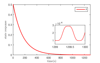
Figure 1: Example 3.1: Trajectory of the estimate $\hat{\theta}$

Example 3.2. ($2\mathrm{D}$ static map) Consider an autonomous vehicle in an environment without GPS orientation [19]. The goal is to reach the the origin, i.e. location of the stationary minimum of a measured distance function

$$\left.\begin{array}[c]{l}J(x(t),y(t))=Q^{\ast}+\frac{1}{2}\left[\begin{array}[c]{cc}x(t)&y(t)\end{array}\right]H\left[\begin{array}[c]{c}x(t)\\ y(t)\end{array}\right]\\ \text{ \ \ \ \ \ \ \ \ \ \ \ \ \ \ \ \ }=x^{2}(t)+y^{2}(t),\end{array}\right.$$

where $Q^{\ast}=0$ and $H=[2,0;0,2].$ We employ the classical ES with measurement and input delays:

$$\left.\begin{array}[c]{l}x(t)=\hat{x}(t)+a_{1}\sin\left(\frac{2\pi l_{1}}{\varepsilon}t\right),\\ y(t)=\hat{y}(t)+a_{2}\sin\left(\frac{2\pi l_{2}}{\varepsilon}t\right),\\ \dot{\hat{x}}(t)=\frac{2k_{1}}{a_{1}}\sin\left(\frac{2\pi l_{1}}{\varepsilon}t\right)J(t-D_{1}(t)),\\ \dot{\hat{y}}(t)=\frac{2k_{2}}{a_{2}}\sin\left(\frac{2\pi l_{2}}{\varepsilon}t\right)J(t-D_{2}(t)),\end{array}\right.$$

where $D_{i}(t)=D_{i}^{\mathrm{in}}+D+\Delta D(t)$ ($i=1,2$) with $\left|\Delta D(t)\right|\leq\rho=\mu\varepsilon$. We select the delays and tuning parameters as

$$\left.\begin{array}[c]{l}D_{1}^{\mathrm{in}}=0.5,\text{ }D_{2}^{\mathrm{in}}=1,\text{ }D=1,\\ k_{1}=k_{2}=-0.003,\text{ }a_{1}=a_{2}=0.3.\end{array}\right.$$ (55)

Following (22), we choose

$$\left.\varepsilon=\frac{1}{2q},\text{ }q\in\mathbf{N}.\right.$$ (56)

To calculate UB, we also choose $\beta=\gamma=0.001$ following Remark 7. Verifying conditions of Theorem 1 ($[\tilde{x}(t),\tilde{y}(t)]^{\mathrm{T}}=[\tilde{\vartheta}_{1}(t),\tilde{\vartheta}_{2}(t)]^{\mathrm{T}}$ since $U=I_{2}$), we arrive at the results shown in Table 2, in which the UB ($\mathrm{\bar{B}}_{i},$ $i=1,2$) corresponds to $\varepsilon=1/4$ $(<\varepsilon^{\ast}=0.3).$

For the numerical simulations, we choose $\varepsilon=1/4,$ $\mu=0.005,$ $\Delta D(t)=\rho\sin t$ with $\rho=\varepsilon\mu=0.125\cdot 10^{-2}$ and the other parameters as shown in (55). Under the initial condition $\hat{x}(s)=-\hat{y}(s)=0.5,$ $s\in[0,2+\rho]$ (thus $[\tilde{x}(s),\tilde{y}(s)]^{\mathrm{T}}=[0.5,-0.5]^{\mathrm{T}},$ $s\in[0,2+\rho]$), the simulation results are shown in Fig. 2, from which we can see that the values of UB shown in Table 2 are confirmed.

Table 2: Example 3.2 with (55): The values of $\mu$, $\varepsilon^{\ast}$, $\omega^{\ast}=2\pi/\varepsilon^{\ast}$, $\delta_{i}$ (i=1,2) and UB ($\mathrm{\bar{B}}_{i},$ $i=1,2$)

ES: sine	$\bar{\sigma}_{01}/\bar{\sigma}_{02}$	$\bar{\sigma}_{1}/\bar{\sigma}_{2}$	$\mu$	$\varepsilon^{\ast}$	$\omega^{\ast}$	$\delta_{1}=\delta_{2}$	$\mathrm{\bar{B}}_{1}/\mathrm{\bar{B}}_{2}$
Theorem 1	0.5/0.5	1/1	$0.005$	0.30	20.94	$0.006$	$0.124/0.124$

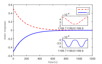
Figure 2: Example 3.2: Trajectories of the estimate ($\hat{x},\hat{y}$)

Example 3.3. ($2\mathrm{D}$ static map) Following [12, 15], we consider the static map (4) with

$$\left.Q^{\ast}=1,\text{ }\theta^{\ast}=\left[\begin{array}[c]{c}0\\ 1\end{array}\right],\text{ }\bar{H}=\left[\begin{array}[c]{cc}-2&-2\\ -2&-4\end{array}\right],\left\|\Delta H\right\|\leq\kappa.\right.$$ (57)

We find that

$$U=\left[\begin{array}[c]{cc}0.5257&0.8507\\ -0.8507&0.5257\end{array}\right]$$

satisfies $U^{\mathrm{T}}U=I_{2}$, $\left\|U\right\|=1$ and

$$UHU^{\mathrm{T}}=\left[\begin{array}[c]{cc}-5.2361&0\\ 0&-0.7639\end{array}\right].$$

We consider two cases: $\kappa=0$ and $\kappa=0.2.$ We choose the delays $D_{i}(t)=D_{i}^{\mathrm{in}}+D+\varepsilon\Delta D(t)$ ($i=1,2$) and the tuning parameters as

$$\left.\begin{array}[c]{l}D_{1}^{\mathrm{in}}=0.5,\text{ }D_{2}^{\mathrm{in}}=1.5,\text{ }D=1,\\ \left|\Delta D(t)\right|\leq\rho=\mu\varepsilon,\text{ }a_{1}=a_{2}=0.3,\\ k_{1}=0.2\cdot 10^{-3},\text{ }k_{2}=0.135\cdot 10^{-2}.\end{array}\right.$$ (58)

Following (22), we choose $\varepsilon$ as in (56). Via Remark 7, we choose $\beta=\gamma=0.001$ to calculate UB ($\mathrm{\bar{B}}_{i}$ for $\tilde{\vartheta}_{i}(t)$, $\mathrm{B}_{i}$ for $\tilde{\theta}_{i}(t),$ $i=1,2$). The results that follow from Theorem 1 for known ($\kappa=0$) and uncertain ($\kappa=0.2$) $H$ are shown in Table 3, in which UB ($\mathrm{\bar{B}}_{i},$ $i=1,2$) corresponds to $\varepsilon=1/4$ $(<\varepsilon^{\ast}=0.49)$ and $\varepsilon=1/8$ $(<\varepsilon^{\ast}=0.016)$ for known and uncertain $H,$ respectively.

For the numerical simulations, we choose $\varepsilon=1/4,$ $\mu=0.003,$ $\Delta D(t)=\rho\sin t$ with $\rho=\varepsilon\mu=0.75\cdot 10^{-2}$ and the other parameter values as shown in (57) and (58). For the real-time estimate $\hat{\theta}(t)$ with the estimation error $\tilde{\theta}(t),$ following part (ii) of Theorem 1, we solve

$$\left.\begin{array}[c]{l}0.5257\sigma_{01}+0.8507\sigma_{02}=0.5,\\ 0.8507\sigma_{01}+0.5257\sigma_{02}=0.5,\end{array}\right.$$ (59)

to obtain $\sigma_{01}=\sigma_{02}=0.3633,$ and the UB ($\mathrm{B}_{i},$ $i=1,2$) can be calculated as

$$\left.\begin{array}[c]{l}\mathrm{B}_{1}=0.5257\cdot 0.023+0.8507\cdot 0.16=0.1482,\\ \mathrm{B}_{2}=0.8507\cdot 0.023+0.5257\cdot 0.16=0.1037.\end{array}\right.$$ (60)

Under the initial condition $\hat{\theta}(s)=[0.3,0.7]^{\mathrm{T}},$ $s\in[0,2+\rho]$ (thus $\tilde{\theta}(s)=\hat{\theta}(s)-\theta^{\ast}=[0.3633,-0.3633]^{\mathrm{T}},$ $s\in[0,2+\rho]$), the simulation results are shown in Fig. 3, from which we can see that the values of UB in (60) are confirmed.

Table 3: Example 3.3 with (58): The values of $\mu$, $\varepsilon^{\ast}$, $\omega^{\ast}=2\pi/\varepsilon^{\ast}$, $\delta_{i}$ (i=1,2) and UB ($\mathrm{\bar{B}}_{i},$ $i=1,2$))

ES: sine	$\bar{\sigma}_{01}/\bar{\sigma}_{02}$	$\bar{\sigma}_{1}/\bar{\sigma}_{2}$	$\mu$	$\varepsilon^{\ast}$	$\omega^{\ast}$	$\delta_{1}=\delta_{2}$	$\mathrm{\bar{B}}_{1}/\mathrm{\bar{B}}_{2}$
Known $H$	0.5/0.5	0.6/1.0	$0.003$	0.49	12.82	$0.001$	0.023/0.16
Uncertain $H$	0.5/0.5	0.6/1.0	$0.001$	0.016	392.70	$0.001$	0.019/0.13

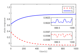
Figure 3: Example 3.3: Trajectories of the estimate ($\hat{\theta_{1}},\hat{\theta_{2}}$)

4 Sampled-data ES with Large Distinct Delays

4.1 Multi-variable static map

In this section, we further study the sampled-data ES with square wave dithers, known large and constant input delays $D_{i}>0$ $(i=1,\ldots,n)$ and periodic fast sampling. Here we assume that $D_{i}/D_{j}$ $(i,j=1,\ldots,n)$ are rational, then there exist some $m_{i}\in\mathbf{N}$ $(i=1,\ldots,n)$ such that

$$m_{i}D_{j}=m_{j}D_{i},\text{ }\forall i,j=1,\ldots,n.$$ (61)

We also choose the corresponding $m_{i}$ $(i=1,\ldots,n)$ as small as possible.

Consider the multi-variable static map $Q(\theta(t))$ in (4) without measurement delay (namely, $D_{\mathrm{out}}(t)=0$), which is measured at the sampling instants $s_{p}$ satisfying $s_{p}=\frac{p\varepsilon}{2^{n}},$ $p\in\mathbf{Z}_{+}$ with a small parameter $\varepsilon>0.$ Let A2-A4 be satisfied. Then equations (7)-(10) hold with $D_{\mathrm{out}}(t)=0$. Define the square wave signal $\mathrm{sq}(t)$ in the following form [26]

$$\left.\mathrm{sq}(t)=\left\{\begin{array}[c]{cl}1,&t\in\left[p,p+\frac{1}{2}\right),\\ -1,&t\in\left[p+\frac{1}{2},1\right),\end{array}\right.p\in\mathbf{Z}_{+}.\right.$$ (62)

We choose the adaptation gain $K$ as (13) such that $K\mathcal{\bar{H}}$ is Hurwitz, and

$$\left.\begin{array}[c]{l}S(t)=[S_{1}(t),\ldots,S_{n}(t)]^{\mathrm{T}},\text{ }S_{i}(t)=a_{i}\mathrm{sq}\left(\frac{l_{i}t}{\varepsilon}\right),\\ M(t)=[M_{1}(t),\ldots,M_{n}(t)]^{\mathrm{T}},\text{ }M_{i}(t)=\frac{1}{a_{i}}\mathrm{sq}\left(\frac{l_{i}t}{\varepsilon}\right)\end{array}\right.$$ (63)

with $l_{i}=2^{i-1},$ $l_{i}\neq l_{j},i\neq j$ and $a_{i}$ are non-zero real numbers. By choosing

$$\left.\varepsilon=\frac{D_{j}}{qm_{j}},\text{ }q\in\mathbf{N}\right.$$ (64)

and using arguments of Lemma 2, we find $\mathrm{sq}(l_{i}(t-D_{j})/\varepsilon)=\mathrm{sq}(l_{i}t/\varepsilon),$ $(i,j=1,\ldots,n).$ Then for $\forall i,j=1,\ldots,n,$

$$\left.S_{i}(t-D_{j})=S_{i}(t),\text{ }M_{i}(t-D_{j})=M_{i}(t).\right.$$ (65)

Let $D_{\text{{M}}}=\max_{i=1,\ldots,n}D_{i}$ and $m=\max_{i=1,\ldots,n}m_{i}.$ Via (61) and (64) we have $D_{\text{{M}}}-D_{i}=\frac{m-m_{i}}{m_{i}}D_{i}=q_{i}\cdot\frac{\varepsilon}{2^{n}}$ and $q_{i}=2^{n}(m-m_{i})q,$ $q\in\mathbf{N}.$

When each signal $\vartheta_{i}$ at the control update instant $t_{p}^{i}$ experiences a constant delay $D_{i}>0$ ($t_{p}^{i}=s_{p}+D_{i}$), the gradient-based sampled-data ES algorithm can be designed as:

$$\left.\dot{\hat{\vartheta}}_{i}(t)=\left\{\begin{array}[c]{ll}0,&t\in[0,D_{\text{{M}}}),\\ k_{i}M_{i}(s_{p})y(s_{p}),&t\in[t_{p}^{i},t_{p+1}^{i}),\end{array}\right.\right.$$ (66)

where $p\geq q_{i},p\in\mathbf{Z}_{+},$ $y(t)=Q(U^{\mathrm{T}}\vartheta(t))$ with $Q(U^{\mathrm{T}}\vartheta(t))$ given by (9) ($D_{\mathrm{out}}(t)=0$) and $\vartheta(t)=\hat{\vartheta}(t)+S(t).$ Via (9), (11) and (66), the estimation error is governed by

$$\left.\begin{array}[c]{l}\dot{\tilde{\vartheta}}_{i}(t)=k_{i}M_{i}(s_{p})Q^{\ast}+\frac{1}{2}k_{i}M_{i}(s_{p})[\tilde{\vartheta}(s_{p})+S(s_{p})]^{\mathrm{T}}\\ \times\mathcal{H}[\tilde{\vartheta}(s_{p})+S(s_{p})],\text{ }t\in[t_{p}^{i},t_{p+1}^{i}),\text{ }p\geq q_{i},\text{ }p\in\mathbf{Z}_{+},\\ \tilde{\vartheta}_{i}(t)=\tilde{\vartheta}_{i}(D_{\text{{M}}}),\text{ }t\in[0,D_{\text{{M}}}].\end{array}\right.$$ (67)

Following the time-delay approach to sampled-data control [5, 26], denote

$$\left.\begin{array}[c]{l}\eta_{i}(t)=t-D_{i}-s_{p},\text{ }t\in[t_{p}^{i},t_{p+1}^{i}),\\ 0\leq\eta_{i}(t)<\frac{\varepsilon}{2^{n}},\text{ }i=1,\ldots,n\mathbf{.}\end{array}\right.$$ (68)

Note that for $\forall i,j=1,\ldots,n,$

$$\left.\mathrm{sq}\left(\frac{l_{j}s_{p}}{\varepsilon}\right)=\mathrm{sq}\left(\frac{l_{j}\left(t-D_{i}\right)}{\varepsilon}\right),\text{ }t\in[t_{p}^{i},t_{p+1}^{i}),\right.$$ (69)

which with (65) implies that

$$\left.\begin{array}[c]{l}M_{j}(s_{p})=M_{j}(t-D_{i})=M_{j}(t),\text{ }t\in[t_{p}^{i},t_{p+1}^{i}),\\ S_{j}(s_{p})=S_{j}(t-D_{i})=S_{j}(t),\text{ }t\in[t_{p}^{i},t_{p+1}^{i}).\end{array}\right.$$ (70)

Taking into account (68) and (70), the dynamics (67) becomes

$$\left.\begin{array}[c]{l}\dot{\tilde{\vartheta}}_{i}(t)=k_{i}M_{i}(t)Q^{\ast}+\frac{1}{2}k_{i}M_{i}(t)[\tilde{\vartheta}(t-D_{i}(t))+S(t)]^{\mathrm{T}}\\ \text{ \ \ \ \ \ \ }\times\mathcal{H}[\tilde{\vartheta}(t-D_{i}(t))+S(t)],\text{ }t\geq D_{\text{{M}}},\text{ }i=1,\ldots,n\mathbf{,}\\ \tilde{\vartheta}_{i}(t)=\tilde{\vartheta}_{i}(D_{\text{{M}}}),\text{ }t\in[0,D_{\text{{M}}}]\end{array}\right.$$ (71)

with

$$D_{i}(t)=D_{i}+\eta_{i}(t).$$ (72)

Recently, for the case of the single input delay $D_{i}=D>0$ ($i=1,\ldots,n$) and the dimension $n=1,2,$ motivated by [6], a time-delay approach for the stability analysis of sampled-data ES algorithms was introduced in [25, 26]. In the latter papers, the ES dynamics was first converted into a neutral type model with a nominal delay-free system, and then the L-K method was used to find sufficient practical stability conditions in the form of LMIs. Different from the treatments for (71) in [25, 26], in this paper we will first transform (71) into a neutral type model with a nominal time-delay system, and further present the resulting neutral system as a retarded one. Finally, motivated by our previous work in [22], we will employ the variation of constants formula to find sufficient practical stability conditions.

As in Section 3, we integrate from $t-\varepsilon$ to $t$ and divide by $\varepsilon$ on both sides of (71) to obtain

$$\left.\begin{array}[c]{l}\frac{1}{\varepsilon}{\textstyle\int\nolimits_{t-\varepsilon}^{t}}\dot{\tilde{\vartheta}}_{i}(\tau)\mathrm{d}\tau=\frac{1}{\varepsilon}{\textstyle\int\nolimits_{t-\varepsilon}^{t}}k_{i}M_{i}(\tau)Q^{\ast}\mathrm{d}\tau\\ +\frac{1}{2\varepsilon}{\textstyle\int\nolimits_{t-\varepsilon}^{t}}k_{i}M_{i}(\tau)S^{\mathrm{T}}(\tau)\mathcal{H}S(\tau)\mathrm{d}\tau\\ +\frac{1}{2\varepsilon}{\textstyle\int\nolimits_{t-\varepsilon}^{t}}k_{i}M_{i}(\tau)\tilde{\vartheta}^{\mathrm{T}}(\tau-D_{i}(\tau))\mathcal{H}\tilde{\vartheta}(\tau-D_{i}(\tau))\mathrm{d}\tau\\ +\frac{1}{\varepsilon}{\textstyle\int\nolimits_{t-\varepsilon}^{t}}k_{i}M_{i}(\tau)S^{\mathrm{T}}(\tau)\mathcal{H}\tilde{\vartheta}(\tau-D_{i}(\tau))\mathrm{d}\tau,\\ \text{ }t\geq D_{\text{{M}}}+\varepsilon,\text{ }i=1,\ldots,n.\end{array}\right.$$ (73)

In view of the definition of $\mathrm{sq}(t)$ in (62) and $l_{i}=2^{i-1},$ $i=1,\ldots,n\mathbf{,}$ we can prove that for $\forall i,j,k=1,\ldots,n\mathbf{,}$

$$\left.\begin{array}[c]{l}{\textstyle\int\nolimits_{t-\varepsilon}^{t}}\mathrm{sq}\left(\frac{l_{i}\tau}{\varepsilon}\right)\mathrm{d}\tau=0,\\ \int_{t-\varepsilon}^{t}\mathrm{sq}\left(\frac{l_{i}\tau}{\varepsilon}\right)\mathrm{sq}\left(\frac{l_{j}\tau}{\varepsilon}\right)\mathrm{sq}\left(\frac{l_{k}\tau}{\varepsilon}\right)\mathrm{d}\tau=0,\text{ }\\ \int\nolimits_{t-\varepsilon}^{t}\frac{a_{i}}{a_{j}}\mathrm{sq}\left(\frac{l_{i}\tau}{\varepsilon}\right)\mathrm{sq}\left(\frac{l_{j}\tau}{\varepsilon}\right)\mathrm{d}\tau=\left\{\begin{array}[c]{cc}\varepsilon,&i=j,\\ 0,&i\neq j.\end{array}\right.\end{array}\right.$$ (74)

Due to (74), relations (25)-(27) hold for $S(t)$ and $M(t)$ defined by (63), $\tilde{\vartheta}(t)=[\tilde{\vartheta}_{1}(t),\ldots,\tilde{\vartheta}_{n}(t)]^{\mathrm{T}}$ satisfying (71) and $D_{i}(t)$ given by (72). Let $G_{i}(t)$ be of the form of (28)-(29). Then we can present

$$\left.\begin{array}[c]{l}\frac{1}{\varepsilon}{\textstyle\int\nolimits_{t-\varepsilon}^{t}}\dot{\tilde{\vartheta}}_{i}(\tau)\mathrm{d}\tau=\frac{\mathrm{d}}{\mathrm{d}t}\left[\tilde{\vartheta}_{i}(t)-G_{i}(t)\right].\end{array}\right.$$ (75)

Substituting (25)-(27) and (75) into (73) and employing notations (31) and (32), we finally arrive at

$$\left.\begin{array}[c]{l}\dot{z}_{i}(t)=k_{i}\bar{h}_{i}z_{i}(t-D_{i}(t))\\ \text{ \ \ \ \ \ \ \ \ }+\bar{w}_{i}(t),\text{ }t\geq D_{\text{{M}}}+\varepsilon,\text{ }i=1,\ldots,n,\\ \bar{w}_{i}(t)=k_{i}\bar{h}_{i}G_{i}(t-D_{i}(t))-Y_{1i}(t)\\ \text{ \ \ \ }\ \ \ \ \ -Y_{2i}(t)+Y_{3i}(t).\end{array}\right.$$ (76)

Similar to the arguments in Section 3, we can use the solution representation formula in Lemma 1 for (76) to find the bound on $|z_{i}|,$ and then the bound on $\tilde{\vartheta}_{i}:|\tilde{\vartheta}_{i}|\leq|z_{i}|+|G_{i}|.$ Comparatively to [25, 26], this will greatly simplify the stability analysis process along with the stability conditions, and improve the quantitative bounds on the parameter $\varepsilon$ and time-delays $D_{i}$ $(i=1,\ldots,n)$.

Similar to Theorem 1, we will find $k_{i}$ $(i=1,\ldots,n)$ from the inequalities (36) with $\bar{D}_{i}=D_{i}$, which guarantee the exponential stability with a decay rate $\delta_{i}$ in (37) of the averaged system (38).

Theorem 2.

Assume A1-A3 hold. Let $k_{i}$ $(i=1,\ldots,n)$ satisfy (36) with $\bar{D}_{i}=D_{i}$. Given tuning parameters $a_{i}$ $(i=1,\ldots,n)$ and $\kappa\geq 0$ as well as $\bar{\sigma}_{i}>\bar{\sigma}_{0i}>0$ $(i=1,\ldots,n)$, let there exists $\varepsilon^{\ast}>0$ that satisfy

$$\left.\begin{array}[c]{l}\Phi_{1}^{i}=\left|k_{i}\bar{h}_{i}\right|D_{i\mathrm{M}}(\varepsilon^{\ast})-\frac{1}{\mathrm{e}}\leq 0,\text{ }i=1,\ldots,n\mathbf{,}\\ \Phi_{2}^{i}=\mathrm{e}^{\left|k_{i}\bar{h}_{i}\right|D_{i\mathrm{M}}(\varepsilon^{\ast})}\left[\bar{\sigma}_{0i}+\frac{3\varepsilon^{\ast}\left|k_{i}\right|\Delta_{1}}{2\left|a_{i}\right|}+\frac{W_{i}(\varepsilon^{\ast},\kappa)}{\left|k_{i}\bar{h}_{i}\right|}\right]\\ \text{ \ \ \ \ }+\frac{\varepsilon^{\ast}\left|k_{i}\right|\Delta_{1}}{2\left|a_{i}\right|}-\bar{\sigma}_{i}<0,\text{ }i=1,\ldots,n\mathbf{,}\end{array}\right.$$ (77)

where

$$\left.\begin{array}[c]{l}D_{i\mathrm{M}}=D_{i\mathrm{M}}(\varepsilon)=D_{i}+\frac{\varepsilon}{2^{n}},\text{ }i=1,\ldots,n\mathbf{,}\\ W_{i}(\varepsilon,\kappa)=\frac{\varepsilon\left|k_{i}\right|}{\left|a_{i}\right|}\left(\frac{\left|k_{i}\bar{h}_{i}\right|}{2}\Delta_{1}+\tilde{\Delta}_{1}+\tilde{\Delta}_{2}\right)+\kappa\left|k_{i}\right|\sqrt{{\textstyle\sum\limits_{j=1}^{n}}\bar{\sigma}_{j}^{2}},\\ \tilde{\Delta}_{1}=\frac{\left(2^{n-1}+1\right)\Delta_{1}}{2^{n}}\left({\textstyle\sum\limits_{j=1}^{n}}\frac{\left|\bar{h}_{j}k_{j}\right|\bar{\sigma}_{j}}{\left|a_{j}\right|}+\kappa\sqrt{{\textstyle\sum\limits_{j=1}^{n}}\bar{\sigma}_{j}^{2}}\sqrt{{\textstyle\sum\limits_{j=1}^{n}}\frac{k_{j}^{2}}{a_{j}^{2}}}\right),\\ \tilde{\Delta}_{2}=\frac{\left(2^{n-1}+1\right)\Delta_{1}}{2^{n}}\left({\textstyle\sum\limits_{j=1}^{n}}\left|\bar{h}_{j}k_{j}\right|+\kappa\sqrt{{\textstyle\sum\limits_{j=1}^{n}}\bar{\sigma}_{j}^{2}}\sqrt{{\textstyle\sum\limits_{j=1}^{n}}\frac{k_{j}^{2}}{a_{j}^{2}}}\right)\end{array}\right.$$

with $\Delta_{1}$ given by (39). Then for all $\varepsilon\in(0,\varepsilon^{\ast}]$ satisfying (64), the following holds:

(i) Solutions of (71) with $|\tilde{\vartheta}_{i}(D_{\mathrm{M}})|\leq\bar{\sigma}_{0i}$ satisfying the following bounds:

$$\left.\begin{array}[c]{l}|\tilde{\vartheta}_{i}(t)|<\left|\tilde{\vartheta}_{i}(D_{\mathrm{M}})\right|+\frac{\varepsilon\left|k_{i}\right|\Delta_{1}}{\left|a_{i}\right|}<\bar{\sigma}_{i},\text{ }t\in[D_{\mathrm{M}},D_{\mathrm{M}}+\varepsilon],\\ |\tilde{\vartheta}_{i}(t)|<\left(1+\left|k_{i}\bar{h}_{i}\right|D_{i\mathrm{M}}\right)\left[\left|\tilde{\vartheta}_{i}(D_{\mathrm{M}})\right|+\frac{3\varepsilon\left|k_{i}\right|\Delta_{1}}{2\left|a_{i}\right|}\right]\\ \text{ \ \ \ \ \ \ \ \ \ }+D_{i\mathrm{M}}W_{i}(\varepsilon,\kappa)+\frac{\varepsilon\left|k_{i}\right|\Delta_{1}}{2\left|a_{i}\right|}\\ \text{ \ \ \ \ \ \ \ }<\bar{\sigma}_{i},\text{ }t\in[D_{\mathrm{M}}+\varepsilon,D_{\mathrm{M}}+D_{i\mathrm{M}}+\varepsilon],\\ |\tilde{\vartheta}_{i}(t)|<\mathrm{e}^{-\left|k_{i}\bar{h}_{i}\right|\left(t-D_{\mathrm{M}}-2D_{i\mathrm{M}}-\varepsilon\right)}\left[\left|\tilde{\vartheta}_{i}(D_{\mathrm{M}})\right|+\frac{3\varepsilon\left|k_{i}\right|\Delta_{1}}{2\left|a_{i}\right|}\right]\\ \text{ \ \ \ \ \ \ \ \ }+\frac{\mathrm{e}^{\left|k_{i}\bar{h}_{i}\right|D_{i\mathrm{M}}}}{\left|k_{i}\bar{h}_{i}\right|}W_{i}(\varepsilon,\kappa)+\frac{\varepsilon\left|k_{i}\right|\Delta_{1}}{2\left|a_{i}\right|}\\ \text{ \ \ \ \ \ \ }<\bar{\sigma}_{i},\text{ }t\geq D_{\mathrm{M}}+D_{i\mathrm{M}}+\varepsilon.\end{array}\right.$$

These solutions are exponentially attracted to the box

$$\left.\begin{array}[c]{c}|\tilde{\vartheta}_{i}(t)|<\Theta_{i}\triangleq\frac{\mathrm{e}^{\left|k_{i}\bar{h}_{i}\right|D_{i\mathrm{M}}}}{\left|k_{i}\bar{h}_{i}\right|}W_{i}(\varepsilon,\kappa)+\frac{\varepsilon\left|k_{i}\right|\Delta_{1}}{2\left|a_{i}\right|},\\ i=1,\ldots,n\end{array}\right.$$ (78)

with decay rates $\delta_{i}=\left|k_{i}\bar{h}_{i}\right|$, which are independent of $\varepsilon$ and delays $D_{i}(t).$

(ii) Consider $\hat{\theta}(t)=U^{\mathrm{T}}\hat{\vartheta}(t)$ with $U=[b_{ij}]_{n\times n},$ where $\hat{\vartheta}(t)$ is defined by (66). Then the estimation errors $\tilde{\theta}_{i}(t)=\hat{\theta}_{i}(t)-\theta^{\ast}$ such that $|\tilde{\theta}_{i}(D_{\mathrm{M}})|\leq\sigma_{0i}$ with ${\textstyle\sum\nolimits_{i=1}^{n}}|b_{ji}|\sigma_{0i}=\bar{\sigma}_{0j}$ $(j=1,\ldots,n\mathbf{)}$ are exponentially attracted to the box $|\tilde{\theta}_{i}(t)|<\sum_{j=1}^{n}b_{ji}\Theta_{j}$ $(i=1,\ldots,n)$ with a decay rate $\delta=\min_{i=1,\ldots,n}\delta_{i}=\min_{i=1,\ldots,n}\left|k_{i}\bar{h}_{i}\right|,$ where $\Theta_{j}$ is defined by (78).

Proof.

The proof is similar to that of Theorem 1 and omitted. ∎

Remark 9.

For the single input delay $D_{i}=D>0$ $(i=1,\ldots,n)$, by using (69) we have $S(s_{p})=S(t-D),M(s_{p})=M(t-D),t\in[t_{p},t_{p+1})$ with $S(t)$ and $M(t)$ given by (63). Note that the equations in (74) still hold with $\tau$ replaced by $\tau-D.$ Thus, the result of Theorem 2 holds for all $\varepsilon\in(0,\varepsilon^{\ast}],$ since there is no need to use (64).

Remark 10.

In [26], the single input delay $D$ was treated under restrictive assumption that $D=$O$(\varepsilon)$ with $\varepsilon$ being a small parameter. Comparatively to that, our results in Theorem 2 not only allow distinct $D_{i},$ but also allow $D_{i}$ to be essentially larger with arbitrary large constant $\bar{D}_{i}$. Actually, Theorem 2 guarantees for any $D_{i}\geq 0$ semi-global convergence for small enough $\varepsilon^{\ast}$ and $\kappa.$ Moreover, Theorem 2 presents much simpler stability conditions, which allow to get larger decay rate and period of the dither signal in the numerical examples. Our UB on the estimation error in (78) is of the order of $\mathrm{O}(\varepsilon)$ provided that $\kappa=0$ and $a_{i},k_{i}$ $(i=1,\ldots,n)$ are of the order of $\mathrm{O}(1).$ This is smaller than $\mathrm{O}(\sqrt{\varepsilon})$ achieved in [26]. In addition, [26] has no results for the uncertain $H$. As a comparison, by using the presented time-delay approach, we can easily solve the uncertainty case.

Parallel to Corollary 1, we have:

Corollary 3.

Assume that A2-A4 hold. Given any $D_{i}>0$ $(i=1,\ldots,n)$ and $\bar{\sigma}_{0i}$ $>0$ (also $\sigma_{0i}>0$) $(i=1,\ldots,n),$ and choosing $k_{i}$ $(i=1,\ldots,n)$ to satisfy (36) with $\bar{D}_{i}=D_{i}$, the ES algorithm converges for small enough $\varepsilon^{\ast}$ and $\kappa.$

4.2 Single-variable static map

Finally, we consider the single-variable static map (44) with A2’, A3, (45) and large known input delay $D>0.$ Let the dither signals $S(t)$ and $M(t)$ satisfy

$$\left.S(t)=a\cdot\mathrm{sq}\left(\frac{t}{\varepsilon}\right),\text{ }M(t)=\frac{1}{a}\cdot\mathrm{sq}\left(\frac{t}{\varepsilon}\right)\right.$$

with $\varepsilon$ being a small parameter, and {$s_{p}$}, {$t_{p}$} denote the sampling and control update instants, respectively, satisfying

$$\left.s_{p}=\frac{p\varepsilon}{2},\text{ }t_{p}=s_{p}+D,\text{ }p\in\mathbf{Z}_{+}.\right.$$

The ES algorithm is designed as

$$\left.\dot{\hat{\theta}}(t)=\left\{\begin{array}[c]{ll}0,&t\in[0,D),\\ kM(s_{p})y(s_{p}),&t\in[t_{p},t_{p+1})\text{ },p\in\mathbf{Z}_{+},\end{array}\right.\right.$$ (79)

where $y(t)=Q(\theta(t))$ with $Q(\theta(t))$ given by (44) and $\theta(t)=\hat{\theta}(t)+S(t).$ Denote

$$\left.\eta(t)=t-D-s_{p},\text{ }t\in[t_{p},t_{p+1}),\text{ }0\leq\eta(t)<\frac{\varepsilon}{2^{n}}.\right.$$ (80)

In addition, we can present

$$\left.M(s_{p})=M(t-D),\text{ }S(s_{p})=S(t-D),\text{ }t\in[t_{p},t_{p+1}).\right.$$ (81)

Taking into account (79)-(81), the estimation error $\tilde{\theta}(t)=\hat{\theta}(t)-\theta^{\ast}$ is governed by

$$\left.\begin{array}[c]{l}\dot{\tilde{\theta}}(t)=kM(t-D)Q^{\ast}+\frac{1}{2}khM(t-D)\\ \text{ \ \ \ \ \ \ \ \ }\times[S(t-D)+\tilde{\theta}(t-D(t))]^{2},\text{ }t\geq D,\\ \tilde{\theta}(t)=\tilde{\theta}(D),\text{ }t\in[0,D].\end{array}\right.$$ (82)

Applying the time-delay approach to averaging of (82), we finally arrive at

$$\left.\begin{array}[c]{l}\dot{z}(t)=khz(t-D(t))+\bar{w}(t),\text{ }t\geq D+\varepsilon,\text{ }i\in\mathbf{I[}1,n\mathbf{]},\\ \bar{w}(t)=khG(t-D(t))-Y_{1}(t)-Y_{2}(t)\end{array}\right.$$

with $\{z(t),G(t),Y_{1}(t),Y_{2}(t)\}$ satisfying updated (32), (28) and (31), respectively.

Similar to Corollary 2, we will find $k$ from the inequality (48) with $D^{\mathrm{in}}+D=D$, which guarantees the exponential stability with a decay rate $\delta$ in (49) of the averaged system (50).

Corollary 4.

Assume that A2’, A3 and (45) hold. let $k$ satisfy (48) with $D^{\mathrm{in}}+D=D$. Given tuning parameters $a$ and $\sigma>\sigma_{0}>0$, let there exists $\varepsilon^{\ast}>0$ that satisfy

$$\left.\begin{array}[c]{l}\Phi_{1}=\left|k\right|h_{\mathrm{M}}\left(D+\frac{\varepsilon^{\ast}}{2}\right)-\frac{1}{\mathrm{e}}\leq 0\mathbf{,}\\ \Phi_{2}=\mathrm{e}^{\left|k\right|h_{\mathrm{M}}\left(D+\varepsilon^{\ast}/2\right)}\left[\sigma_{0}+\frac{3\varepsilon^{\ast}\Delta}{4}+W(\varepsilon^{\ast})\right]\\ \text{ \ \ \ \ }+\frac{\varepsilon^{\ast}\Delta}{4}-\sigma<0\mathbf{,}\end{array}\right.$$

where

$$\left.W(\varepsilon)=\frac{\varepsilon\Delta}{4}\left(3+\frac{2\sigma}{\left|a\right|}\right)\right.$$

and $\Delta$ is given in (52). Then for all $\varepsilon\in(0,\varepsilon^{\ast}],$ the solution $\tilde{\theta}(t)$ with $|\tilde{\theta}(D)|\leq\sigma_{0}$ satisfies

$$\left.\begin{array}[c]{l}|\tilde{\theta}(t)|<\left|\tilde{\theta}(D)\right|+\frac{\varepsilon}{2}\Delta<\sigma,\text{ }t\in[D,D+\varepsilon],\\ |\tilde{\theta}(t)|<\left[1+\left|k\right|h_{\mathrm{M}}\left(D+\frac{\varepsilon}{2}\right)\right]\left[\left|\tilde{\theta}(D)\right|+\frac{3\varepsilon\Delta}{4}\right]\\ \text{ \ \ \ \ \ \ \ \ \ }+\left(D+\frac{\varepsilon}{2}\right)\left|k\right|h_{\mathrm{M}}W(\varepsilon)+\frac{\varepsilon\Delta}{4}\\ \text{ \ \ \ \ \ \ \ }<\sigma,\text{ }t\in\left[D+\varepsilon,2D+\frac{3\varepsilon}{2}\right].\\ |\tilde{\theta}(t)|<\mathrm{e}^{-\left|k\right|h_{\mathrm{m}}\left(t-2D-3\varepsilon/2\right)}\mathrm{e}^{\left|k\right|h_{\mathrm{M}}\left(D+\varepsilon/2\right)}\left[\left|\tilde{\vartheta}(D)\right|+\frac{3\varepsilon\Delta}{4}\right]\\ \text{ \ \ \ \ \ \ \ \ \ }+\mathrm{e}^{\left|k\right|h_{\mathrm{M}}\left(D+\varepsilon/2\right)}W(\varepsilon)+\frac{\varepsilon\Delta}{4}\\ \text{ \ \ \ \ \ \ \ }<\sigma,\text{ }t\geq 2D+\frac{3\varepsilon}{2}.\end{array}\right.$$

This solution is exponentially attracted to the interval

$$\left.|\tilde{\theta}(t)|<\mathrm{e}^{\left|k\right|h_{\mathrm{M}}\left(D+\varepsilon/2\right)}W(\varepsilon)+\frac{\varepsilon\Delta}{4}\right.$$

with a decay rate $\delta=\left|k\right|h_{\mathrm{m}}.$

4.3 Examples

Example 4.1. ($1\mathrm{D}$ static map) Consider the single-input map (44) with

$$Q^{\ast}=0,\text{ }h=2.$$ (83)

Note that

$$\left.\begin{array}[c]{ll}\dot{\hat{\theta}}(t)=ka\cdot\mathrm{sq}(\frac{t}{\varepsilon})y(t)&\text{in \cite[cite]{[\@@bibref{}{zfo21cdc}{}{}]},}\\ \dot{\hat{\theta}}(t)=\frac{k}{a}\cdot\mathrm{sq}(\frac{t}{\varepsilon})y(t)&\text{in Corollary \ref{corollary3}.}\end{array}\right.$$

For a fair comparison, we select the tuning parameters of the gradient-based ES as

$$\left.\begin{array}[c]{ll}a=0.1,\text{ }k=-1.3&\text{in \cite[cite]{[\@@bibref{}{zfo21cdc}{}{}]},}\\ a=0.1,\text{ }k=-1.3\cdot 0.1^{2}=-0.013&\text{in Corollary \ref{corollary3}.}\end{array}\right.$$ (84)

If $Q^{\ast}$ and $h$ are uncertain and satisfy A3 and (45), respectively, we consider

$$\left|Q^{\ast}\right| \leq 0.1,\text{ }1.9\leq\left|h\right|\leq 2.1;$$ (85)

$$\left|Q^{\ast}\right| \leq 1.0,\text{ }1.0\leq\left|h\right|\leq 3.0.$$ (86)

The results that follow from Theorem 2, Corollary 4 and [25] are shown in Table 4. It follows that our results allow larger decay rate $\delta$, larger upper bound $\varepsilon^{\ast}$ (small lower bound frequency $\omega^{\ast}$), much larger time-delay $D$ and much smaller UB than those in [25]. Moreover, our results allow much larger uncertainties in $Q^{\ast}$ and $h$ than those in [25].

Table 4: Example 4.1: Comparison of $\delta$, $D$, $\varepsilon^{\ast}$, $\omega^{\ast}=2\pi/\varepsilon^{\ast}$ and UB

ES: square	$\sigma_{0}$	$\sigma$	$\delta$	$D$	$\varepsilon^{\ast}$	$\omega^{\ast}$	UB
Corollary 4 with (83)	1	$\sqrt{2}$	0.026	1.0	0.071	88.49	$2.7\cdot\mathrm{10}^{-4}$
Theorem 2 with (83)	1	$\sqrt{2}$	0.026	1.0	0.071	88.49	$2.7\cdot\mathrm{10}^{-4}$
[25] with (83)	1	$\sqrt{2}$	0.02	0.01	0.045	139.63	0.04
Corollary 4 with (85)	1	$\sqrt{2}$	0.0247	1.0	0.065	96.66	$2.0\cdot\mathrm{10}^{-3}$
Theorem 2 with (85)	1	$\sqrt{2}$	0.026	0.5	0.052	120.83	$1.9\cdot\mathrm{10}^{-3}$
[25] with (85)	1	$\sqrt{2}$	0.02	0.01	0.036	174.53	0.22
Corollary 4 with (86)	1	$\sqrt{2}$	0.013	1.0	0.035	179.52	$1.1\cdot\mathrm{10}^{-2}$
Theorem 2 with (86)	1	$\sqrt{2}$	-	-	-	-	-
[25] with (86)	1	$\sqrt{2}$	-	-	-	-	-

Example 4.2. ($2\mathrm{D}$ static map) We consider the Example 3.2 in Section 3.3 with $D_{i}=D$ ($i=1,2$) and the parameters chosen as [26]:

$$k_{1}=k_{2}=-0.01,{\ }a_{1}=a_{2}=0.2.$$ (87)

Verifying conditions of Theorem 2 and [26], we arrive at results shown in Table 5, in which UB$=($B̄${}_{1}^{2}+$B̄${}_{2}^{2})^{1/2}$ with B̄₁ and B̄₂ be the ultimate bound values of $\tilde{x}(t)$ and $\tilde{y}(t)$, respectively. By comparing the data, we find that our results in Theorem 2 allow larger decay rate $\delta$, larger upper bound $\varepsilon^{\ast}$ (small lower bound frequency $\omega^{\ast}$), much larger time-delay $D$ and much smaller UB than those in [26].

Table 5: Example 4.2 with (87): Comparison of $\delta$, $D$, $\varepsilon^{\ast}$, $\omega^{\ast}=2\pi/\varepsilon^{\ast}$ and UB

ES: square	$\bar{\sigma}_{01}/\bar{\sigma}_{02}$	$\bar{\sigma}_{1}/\bar{\sigma}_{2}$	$\delta$	$D$	$\varepsilon^{\ast}$	$\omega^{\ast}$	UB
Theorem 2	1/1	2/2	$0.02$	$2$	0.1	62.83	$1.6\cdot\mathrm{10}^{-3}$
[26]	1/1	2/2	$0.01$	$0.01$	0.09	69.81	0.18

Example 4.3 ($2\mathrm{D}$ static map) We consider the Example 3.3 in Section 3.3 with the delays and tuning parameters chosen as

$$\left.\begin{array}[c]{l}D_{1}=1.5,\text{ }D_{2}=2.5,\text{ }a_{1}=a_{2}=0.3,\\ k_{1}=0.6\cdot 10^{-3},\text{ }k_{2}=0.4\cdot 10^{-2}.\end{array}\right.$$ (88)

Following (64), we choose $\varepsilon$ as in (56). The results that follow from Theorem 2 are shown in Table 6, in which UB ($\mathrm{\bar{B}}_{i},$ $i=1,2$) corresponds to $\varepsilon=1/2$ $(<\varepsilon^{\ast}=0.79)$ and $\varepsilon=1/4$ $(<\varepsilon^{\ast}=0.36)$ for known ($\kappa=0$) and uncertain ($\kappa=0.2$) $H,$ respectively. It follows that Theorem 2 works well.

Table 6: Example 4.3 with (88): The values of $\varepsilon^{\ast}$, $\omega^{\ast}(2\pi/\varepsilon^{\ast})$, $\delta_{i}$ (i=1,2) and UB ($\mathrm{\bar{B}}_{i},$ $i=1,2$)

ES: square	$\bar{\sigma}_{01}/\bar{\sigma}_{02}$	$\bar{\sigma}_{1}/\bar{\sigma}_{2}$	$\varepsilon^{\ast}$	$\omega^{\ast}$	$\delta_{1}=\delta_{2}$	$\mathrm{\bar{B}}_{1}/\mathrm{\bar{B}}_{2}$
Known $H$	0.5/0.5	0.6/1.0	0.79	7.95	$0.031$	$4.1\cdot\mathrm{10}^{-3}$/$2.8\cdot\mathrm{10}^{-2}$
Uncertain $H$	0.5/0.5	0.6/1.0	0.36	17.45	$0.031$	$5.0\cdot\mathrm{10}^{-3}$/$3.4\cdot\mathrm{10}^{-2}$

For the real-time estimate $\hat{\theta}(t)$ with the estimation error $\tilde{\theta}(t),$ following part (ii) of Theorem 2, we solve (59) to obtain

$$\left.\sigma_{01}=\sigma_{02}=0.3633,\right.$$

and the UB ($\mathrm{B}_{i}$ for $\tilde{\theta}_{i}(t),$ $i=1,2$) can be calculated as

$$\left.\begin{array}[c]{l}\mathrm{B}_{1}=0.5257\cdot\mathrm{\bar{B}}_{1}+0.8507\cdot\mathrm{\bar{B}}_{2}=2.6\cdot 10^{-2},\\ \mathrm{B}_{2}=0.8507\cdot\mathrm{\bar{B}}_{1}+0.5257\cdot\mathrm{\bar{B}}_{2}=1.82\cdot 10^{-2}.\end{array}\right.$$

5 Conclusion

This paper developed a time-delay approach to gradient-based ES of uncertain quadratic maps in the presence of large measurement delay and input distinct delays, and sampled-data ES with large distinct input delays. By choosing gains to stabilize averaged time-delay systems, explicit conditions in terms of simple inequalities were established to guarantee the practical stability of the ES control systems. The resulting time-delay method provides a quantitative bounds on the control parameters and the ultimate bound of seeking error. Compared with recent quantitative result on the sampled-data implementation, the presented method not only greatly simplifies the stability conditions and improves the results, but also allow distinct and large time delays. Future work may include the extension to discrete-time ES in the presence of large delays by using the time-delay approach to averaging for discrete-time systems introduced in [21, 22].

Appendix

A1: Proof of Lemma 2

Let

$$\left.i\cdot\omega_{j}=j\cdot\omega_{i},\text{ }\forall i,j=1,\ldots,n\mathbf{.}\right.$$ (89)

For fixed $m_{1},$ we choose

$$\left.\omega_{1}=\frac{q\cdot 2\pi m_{1}}{\bar{D}_{1}},\text{ }q\in\mathbf{N}.\right.$$ (90)

Then via (89), $\omega_{i}$ ($i=2,\ldots,n$) are in forms of

$$\left.\omega_{i}=\frac{q\cdot 2\pi im_{1}}{\bar{D}_{1}},\text{ }q\in\mathbf{N},\text{ }\forall i=2,\ldots,n\mathbf{.}\right.$$ (91)

Combining (90) and (91) gives

$$\left.\omega_{i}=\frac{q\cdot 2\pi im_{1}}{\bar{D}_{1}},\text{ }q\in\mathbf{N},\text{ }\forall i=1,\ldots,n\mathbf{.}\right.$$ (92)

Noting (6), from (92) we further have (17), namely,

$$\left.\omega_{i}\bar{D}_{j}=2\pi\cdot qim_{j},\text{ }q\in\mathbf{N},\text{ }\forall i,j=1,\ldots,n\mathbf{,}\right.$$

which implies (18) since $qim_{j}$ are all positive integers. This completes the proof.

A2: Proof of Theorem 1

Since $\tilde{\theta}(t)=U^{\mathrm{T}}\tilde{\vartheta}(t),$ it is not difficult to obtain part (ii) from part (i). Thus, we just need to prove part (i). The proof is divided into three parts. (A) First, we present a group of upper bounds under the assumption that $\tilde{\vartheta}_{i}(t)$ ($i=1,\ldots,n$) are bounded for $t\geq D_{\mathrm{M}}$; (B) Second, we show the practical stability of each $z_{i}$-system in (33) (and thus each $\tilde{\vartheta}_{i}$-system in (20)); (C) Third, we show the availability of the assumption that $\tilde{\vartheta}_{i}(t)$ are bounded for $t\geq D_{\mathrm{M}}$ by contradiction.

Proof of part A. Assume that

$$\left.|\tilde{\vartheta}_{i}(t)|<\bar{\sigma}_{i},\text{ }i=1,\ldots,n,\text{ }t\geq D_{\mathrm{M}}.\right.$$ (93)

When $t\in[0,D_{\mathrm{M}}],$ we note that $\tilde{\vartheta}_{i}(t)$ ($i=1,\ldots,n$) are constants satisfying

$$\left.|\dot{\tilde{\vartheta}}_{i}(t)|=0,\text{ }|\tilde{\vartheta}_{i}(t)|\leq\bar{\sigma}_{0i}<\bar{\sigma}_{i},\text{ }t\in[0,D_{\mathrm{M}}],\right.$$ (94)

which with (93) yields

$$\left.|\tilde{\vartheta}_{i}(t)|<\bar{\sigma}_{i},\text{ }t\geq 0,\text{ }i=1,\ldots,n\mathbf{,}\right.$$ (95)

and

$$\left.|\tilde{\vartheta}(t)|=\sqrt{{\textstyle\sum\limits_{j=1}^{n}}\tilde{\vartheta}_{j}^{2}(t)}<\sqrt{{\textstyle\sum\limits_{j=1}^{n}}\bar{\sigma}_{j}^{2}},\text{ }t\geq 0.\right.$$ (96)

Employing (9) and (29), we find

$$\left.\begin{array}[c]{l}\text{ \ \ }Q(U^{\mathrm{T}}\vartheta(t-D_{i}(t)))\\ \overset{(\ref{eq11})}{=}Q^{\ast}+\frac{1}{2}{\textstyle\sum\limits_{j=1}^{n}}\bar{h}_{j}\left(\tilde{\vartheta}_{j}(t-D_{i}(t))+S_{j}(t-D_{i}(t))\right)^{2}\\ \text{ \ \ }+\frac{1}{2}\left[\tilde{\vartheta}(t-D_{i}(t))+S(t-D_{i}(t))\right]^{\mathrm{T}}\\ \text{ \ \ }\times\Delta\mathcal{H}\left[\tilde{\vartheta}(t-D_{i}(t))+S(t-D_{i}(t))\right],\\ \text{ \ \ }\bar{Q}(\tilde{\vartheta}(t-D_{i}(t)))\\ \overset{(\ref{eq11})}{=}Q^{\ast}+\frac{1}{2}{\textstyle\sum\limits_{j=1}^{n}}\bar{h}_{j}\left(\tilde{\vartheta}_{j}(t-D_{i}(t))+S_{j}(t)\right)^{2}\\ \text{ \ \ }+\frac{1}{2}\left[\tilde{\vartheta}(t-D_{i}(t))+S(t)\right]^{\mathrm{T}}\\ \text{ \ \ }\times\Delta\mathcal{H}\left[\tilde{\vartheta}(t-D_{i}(t))+S(t)\right].\end{array}\right.$$ (97)

Note from (8), (12) and $\left\|\Delta H(t)\right\|\leq\kappa$ in A3 that

$$\left.\begin{array}[c]{l}\left|S_{i}(t)\right|=\left|a_{i}\right|,\text{ }\left|M_{i}(t)\right|=\frac{2}{\left|a_{i}\right|},\text{ }i=1,\ldots,n\mathbf{,}\\ \left|S^{\mathrm{T}}(t)\right|=\left|S(t)\right|=\sqrt{{\textstyle\sum\limits_{j=1}^{n}}a_{j}^{2}},\\ \left\|\Delta\mathcal{H}(t)\right\|\leq\left\|U\right\|^{2}\left\|\Delta H(t)\right\|\leq\kappa.\end{array}\right.$$ (98)

Then via (95)-(98), we have

$$\left.\begin{array}[c]{l}\text{ \ \ }\left|Q(U^{\mathrm{T}}\vartheta(t-D_{i}(t)))\right|\\ \leq\left|Q^{\ast}\right|+\frac{1}{2}{\textstyle\sum\limits_{j=1}^{n}}\left|\bar{h}_{j}\right||\tilde{\vartheta}_{j}(t-D_{i}(t))+S_{j}(t-D_{i}(t))|^{2}\\ \text{ \ \ }+\frac{1}{2}\left\|\Delta\mathcal{H}\right\||\tilde{\vartheta}(t-D_{i}(t))+S(t-D_{i}(t))|^{2}\\ <\Delta_{1},\text{ }t\geq D_{\mathrm{M}},\\ \text{ \ \ }|\bar{Q}(\tilde{\vartheta}(t-D_{i}(t)))|\\ \leq\left|Q^{\ast}\right|+\frac{1}{2}{\textstyle\sum\limits_{j=1}^{n}}\left|\bar{h}_{j}\right||\tilde{\vartheta}_{j}(t-D_{i}(t))+S_{j}(t)|^{2}\\ \text{ \ \ }+\frac{1}{2}\left\|\Delta\mathcal{H}\right\||\tilde{\vartheta}(t-D_{i}(t))+S(t)|^{2}\\ <\Delta_{1},\text{ }t\geq D_{\mathrm{M}}\end{array}\right.$$ (99)

with $\Delta_{1}$ given in (39), by which, (94) and (98) we further have for $i=1,\ldots,n\mathbf{,}$

$$\left.\left|\dot{\tilde{\vartheta}}_{i}(t)\right|<\frac{2\left|k_{i}\right|\Delta_{1}}{\left|a_{i}\right|},\text{ }t\geq 0,\right.$$ (100)

and then

$$\left.\begin{array}[c]{l}\left|\tilde{\vartheta}_{i}(t)\right|=\left|\tilde{\vartheta}_{i}(D_{\mathrm{M}})+{\textstyle\int\nolimits_{D_{\mathrm{M}}}^{t}}\dot{\tilde{\vartheta}}_{i}(s)\mathrm{d}s\right|\\ <\left|\tilde{\vartheta}_{i}(D_{\mathrm{M}})\right|+\frac{2\varepsilon\left|k_{i}\right|\Delta_{1}}{\left|a_{i}\right|},\text{ }t\in[D_{\mathrm{M}},D_{\mathrm{M}}+\varepsilon].\end{array}\right.$$ (101)

This implies the first inequality in (42) since $\Phi_{2}^{i}<0$ in (40) implies that $\bar{\sigma}_{0i}+\frac{2\varepsilon^{\ast}\left|k_{i}\right|\Delta_{1}}{\left|a_{i}\right|}<\bar{\sigma}_{i}.$ Moreover, employing (100) we have

$$\left.\left|\dot{\tilde{\vartheta}}(t)\right|=\sqrt{{\textstyle\sum\limits_{j=1}^{n}}\dot{\tilde{\vartheta}}_{j}(t)}<2\Delta_{1}\sqrt{{\textstyle\sum\limits_{j=1}^{n}}\frac{k_{j}^{2}}{a_{j}^{2}}},\text{ }t\geq 0.\right.$$ (102)

By using (98) and the second inequality in (99), from (28) we have

$$\left.\begin{array}[c]{l}\left|G_{i}(t)\right|=\left|\frac{1}{\varepsilon}\int\nolimits_{t-\varepsilon}^{t}(\tau-t+\varepsilon)k_{i}M_{i}(\tau)\bar{Q}(\tilde{\vartheta}(\tau-D_{i}(\tau)))\mathrm{d}\tau\right|\\ \text{ \ \ \ \ \ \ \ }\leq\frac{1}{\varepsilon}{\textstyle\int\nolimits_{t-\varepsilon}^{t}}(\tau-t+\varepsilon)\left|k_{i}M_{i}(\tau)\bar{Q}(\tilde{\vartheta}(\tau-D_{i}(\tau)))\right|\mathrm{d}\tau\\ \text{ \ \ \ \ \ \ \ }<\frac{2\left|k_{i}\right|\Delta_{1}}{\varepsilon\left|a_{i}\right|}{\textstyle\int\nolimits_{t-\varepsilon}^{t}}(\tau-t+\varepsilon)\mathrm{d}\tau\\ \text{ \ \ \ \ \ \ \ }=\frac{\varepsilon\left|k_{i}\right|\Delta_{1}}{\left|a_{i}\right|},\text{ }t\geq D_{\mathrm{M}}+\varepsilon,\text{ }i=1,\ldots,n\mathbf{,}\end{array}\right.$$ (103)

this with $G_{i}(t)=0,$ $t\in[\varepsilon,D_{\mathrm{M}}+\varepsilon)$ in (32) gives

$$\left.\begin{array}[c]{l}|k_{i}\bar{h}_{i}G_{i}(t-D_{i}(t))|\leq\left|k_{i}\bar{h}_{i}\right||G_{i}(t-D_{i}(t))|\\ <\frac{\varepsilon k_{i}^{2}\left|\bar{h}_{i}\right|\Delta_{1}}{\left|a_{i}\right|},\text{ }t\geq D_{\mathrm{M}}+\varepsilon,\text{ }i=1,\ldots,n\mathbf{.}\end{array}\right.$$ (104)

Employing (10), (34), (95), (96), (98), (100) and (102), we have from (31) that

$$\left.\begin{array}[c]{l}|Y_{1i}(t)|\leq\frac{1}{\varepsilon}{\textstyle\int\nolimits_{t-\varepsilon}^{t}}{\textstyle\int\nolimits_{\tau-D_{i}(\tau)}^{t-D_{i}(t)}}\left|k_{i}M_{i}(\tau)\right|\left|\tilde{\vartheta}^{\mathrm{T}}(s)\mathcal{H}\dot{\tilde{\vartheta}}(s)\right|\mathrm{d}s\mathrm{d}\tau\\ \text{ \ \ \ \ \ \ \ \ }\leq\frac{2\left|k_{i}\right|}{\varepsilon\left|a_{i}\right|}{\textstyle\int\nolimits_{t-\varepsilon}^{t}}{\textstyle\int\nolimits_{\tau-D_{i}(\tau)}^{t-D_{i}(t)}}{\textstyle\sum\limits_{j=1}^{n}}\left|\bar{h}_{j}\tilde{\vartheta}_{j}(s)\dot{\tilde{\vartheta}}_{j}(s)\right|\mathrm{d}s\mathrm{d}\tau\\ \text{ \ \ \ \ \ \ \ \ \ \ \ }+\frac{2\left|k_{i}\right|}{\varepsilon\left|a_{i}\right|}{\textstyle\int\nolimits_{t-\varepsilon}^{t}}{\textstyle\int\nolimits_{\tau-D_{i}(\tau)}^{t-D_{i}(t)}}\left|\tilde{\vartheta}^{\mathrm{T}}(s)\Delta\mathcal{H}\dot{\tilde{\vartheta}}(s)\right|\mathrm{d}s\mathrm{d}\tau\\ \text{ \ \ \ \ \ \ \ \ }<\frac{4\left|k_{i}\right|\Delta_{1}}{\varepsilon\left|a_{i}\right|}{\textstyle\sum\limits_{j=1}^{n}}\frac{\left|\bar{h}_{j}k_{j}\right|\bar{\sigma}_{j}}{\left|a_{j}\right|}{\textstyle\int\nolimits_{t-\varepsilon}^{t}}{\textstyle\int\nolimits_{\tau-D_{i}(\tau)}^{t-D_{i}(t)}}1\mathrm{d}s\mathrm{d}\tau\\ \text{ \ \ \ \ \ \ \ \ \ \ \ }+\frac{4\kappa\left|k_{i}\right|\Delta_{1}}{\varepsilon\left|a_{i}\right|}\sqrt{{\textstyle\sum\limits_{j=1}^{n}}\bar{\sigma}_{j}^{2}}\sqrt{{\textstyle\sum\limits_{j=1}^{n}}\frac{k_{j}^{2}}{a_{j}^{2}}}{\textstyle\int\nolimits_{t-\varepsilon}^{t}}{\textstyle\int\nolimits_{\tau-D_{i}(\tau)}^{t-D_{i}(t)}}1\mathrm{d}s\mathrm{d}\tau\\ \text{ \ \ \ \ \ \ \ \ }\leq\frac{4\left|k_{i}\right|\Delta_{1}}{\varepsilon\left|a_{i}\right|}\left({\textstyle\sum\limits_{j=1}^{n}}\frac{\left|\bar{h}_{j}k_{j}\right|\bar{\sigma}_{j}}{\left|a_{j}\right|}+\kappa\sqrt{{\textstyle\sum\limits_{j=1}^{n}}\bar{\sigma}_{j}^{2}}\sqrt{{\textstyle\sum\limits_{j=1}^{n}}\frac{k_{j}^{2}}{a_{j}^{2}}}\right)\\ \text{ \ \ \ \ \ \ \ \ \ \ \ }\times{\textstyle\int\nolimits_{t-\varepsilon}^{t}}\left(t-\tau+2\varepsilon\mu\right)\mathrm{d}\tau\\ \text{ \ \ \ \ \ \ \ \ }=\frac{\varepsilon\left|k_{i}\right|}{\left|a_{i}\right|}\bar{\Delta}_{1},\text{ }t\geq D_{\mathrm{M}}+\varepsilon,\text{ }i=1,\ldots,n\end{array}\right.$$ (105)

with $\bar{\Delta}_{1}$ given in (39),

$$\left.\begin{array}[c]{l}|Y_{2i}(t)|\leq\frac{1}{\varepsilon}{\textstyle\int\nolimits_{t-\varepsilon}^{t}}{\textstyle\int\nolimits_{\tau-D_{i}(\tau)}^{t-D_{i}(t)}}\left|k_{i}M_{i}(\tau)\right|\left|S^{\mathrm{T}}(\tau)\mathcal{H}\dot{\tilde{\vartheta}}(s)\right|\mathrm{d}s\mathrm{d}\tau\\ \text{ \ \ \ \ \ \ \ \ }\leq\frac{2\left|k_{i}\right|}{\varepsilon\left|a_{i}\right|}{\textstyle\int\nolimits_{t-\varepsilon}^{t}}{\textstyle\int\nolimits_{\tau-D_{i}(\tau)}^{t-D_{i}(t)}}{\textstyle\sum\limits_{j=1}^{n}}\left|\bar{h}_{j}S_{j}(\tau)\dot{\tilde{\vartheta}}_{j}(s)\right|\mathrm{d}s\mathrm{d}\tau\\ \text{ \ \ \ \ \ \ \ \ \ \ \ }+\frac{2\left|k_{i}\right|}{\varepsilon\left|a_{i}\right|}{\textstyle\int\nolimits_{t-\varepsilon}^{t}}{\textstyle\int\nolimits_{\tau-D_{i}(\tau)}^{t-D_{i}(t)}}\left|S^{\mathrm{T}}(\tau)\Delta\mathcal{H}\dot{\tilde{\vartheta}}(s)\right|\mathrm{d}s\mathrm{d}\tau\\ \text{ \ \ \ \ \ \ \ \ }<\frac{4\left|k_{i}\right|\Delta_{1}}{\varepsilon\left|a_{i}\right|}{\textstyle\sum\limits_{j=1}^{n}}\left|\bar{h}_{j}k_{j}\right|{\textstyle\int\nolimits_{t-\varepsilon}^{t}}{\textstyle\int\nolimits_{\tau-D_{i}(\tau)}^{t-D_{i}(t)}}1\mathrm{d}s\mathrm{d}\tau\\ \text{ \ \ \ \ \ \ \ \ \ \ \ }+\frac{4\kappa\left|k_{i}\right|\Delta_{1}}{\varepsilon\left|a_{i}\right|}\sqrt{{\textstyle\sum\limits_{j=1}^{n}}a_{j}^{2}}\sqrt{{\textstyle\sum\limits_{j=1}^{n}}\frac{k_{j}^{2}}{a_{j}^{2}}}{\textstyle\int\nolimits_{t-\varepsilon}^{t}}{\textstyle\int\nolimits_{\tau-D_{i}(\tau)}^{t-D_{i}(t)}}1\mathrm{d}s\mathrm{d}\tau\\ \text{ \ \ \ \ \ \ \ \ }\leq\frac{4\left|k_{i}\right|\Delta_{1}}{\varepsilon\left|a_{i}\right|}\left({\textstyle\sum\limits_{j=1}^{n}}\left|\bar{h}_{j}k_{j}\right|+\kappa\sqrt{{\textstyle\sum\limits_{j=1}^{n}}\bar{\sigma}_{j}^{2}}\sqrt{{\textstyle\sum\limits_{j=1}^{n}}\frac{k_{j}^{2}}{a_{j}^{2}}}\right)\\ \text{ \ \ \ \ \ \ \ \ \ \ \ }\times{\textstyle\int\nolimits_{t-\varepsilon}^{t}}\left(t-\tau+2\varepsilon\mu\right)\mathrm{d}\tau\\ \text{ \ \ \ \ \ \ \ \ }=\frac{\varepsilon\left|k_{i}\right|}{\left|a_{i}\right|}\bar{\Delta}_{2},\text{ }t\geq D_{\mathrm{M}}+\varepsilon,\text{ }i=1,\ldots,n\end{array}\right.$$ (106)

with $\bar{\Delta}_{2}$ given in (39), and

$$\left.\begin{array}[c]{l}\left|Y_{3i}(t)\right|\leq\left|C(k_{i})\right|\left\|\Delta\mathcal{H}\right\|\left|\tilde{\vartheta}(t-D_{i}(t))\right|\\ \text{ \ \ \ }<\left|k_{i}\right|\kappa\sqrt{{\textstyle\sum\limits_{j=1}^{n}}\bar{\sigma}_{j}^{2}},\text{ }t\geq D_{\mathrm{M}}+\varepsilon,\text{ }i=1,\ldots,n.\end{array}\right.$$ (107)

Noting the form of $S(t)$ in (12) with $\omega_{i}$ satisfying (23) and $\left|\Delta D(t)\right|\leq\rho$ with $\rho$ chosen as (34), we find

$$\left.\begin{array}[c]{l}\left|{\textstyle\int\nolimits_{t-\Delta D(t)}^{t}}\dot{S}_{i}(s)\mathrm{d}s\right|\leq 2\pi\mu i\left|a_{i}\right|,\text{ }i=1,\ldots,n\mathbf{,}\\ \left|{\textstyle\int\nolimits_{t-\Delta D(t)}^{t}}\dot{S}(s)\mathrm{d}s\right|\leq 2\pi\mu\sqrt{{\textstyle\sum\limits_{j=1}^{n}}j^{2}a_{j}^{2}}.\end{array}\right.$$ (108)

Employing (10), (34), (95), (96), (98) and (108), we obtain

$$\left.\begin{array}[c]{l}\text{ \ \ }\left|k_{i}M_{i}(t)S^{\mathrm{T}}(t)\mathcal{H}{\textstyle\int\nolimits_{t-\Delta D(t)}^{t}}\dot{S}(s)\mathrm{d}s\right|\\ \leq\left|k_{i}M_{i}(t)\right|{\textstyle\sum\limits_{j=1}^{n}}\left|\bar{h}_{j}\right|\left|S_{j}(t)\right|\left|{\textstyle\int\nolimits_{t-\Delta D(t)}^{t}}\dot{S}_{j}(s)\mathrm{d}s\right|\\ \text{ \ \ }+\left|k_{i}M_{i}(t)\right|\left\|\Delta\mathcal{H}(t)\right\|\left|S(t)\right|\left|{\textstyle\int\nolimits_{t-\Delta D(t)}^{t}}\dot{S}(s)\mathrm{d}s\right|\\ \leq\frac{4\pi\mu\left|k_{i}\right|}{\left|a_{i}\right|}{\textstyle\sum\limits_{j=1}^{n}}\left|\bar{h}_{j}\right|ja_{j}^{2}+\frac{4\pi\mu\kappa\left|k_{i}\right|}{\left|a_{i}\right|}\sqrt{{\textstyle\sum\limits_{j=1}^{n}}a_{j}^{2}}\sqrt{{\textstyle\sum\limits_{j=1}^{n}}j^{2}a_{j}^{2}},\end{array}\right.$$ (109)

$$\left.\begin{array}[c]{l}\text{ \ \ }\left|\frac{k_{i}M_{i}(t)}{2}\left({\textstyle\int\nolimits_{t-\Delta D(t)}^{t}}\dot{S}(s)\mathrm{d}s\right)^{\mathrm{T}}\mathcal{H}\left({\textstyle\int\nolimits_{t-\Delta D(t)}^{t}}\dot{S}(s)\mathrm{d}s\right)\right|\\ \leq\frac{\left|k_{i}M_{i}(t)\right|}{2}{\textstyle\sum\limits_{j=1}^{n}}\left|\bar{h}_{j}\right|\left|{\textstyle\int\nolimits_{t-\Delta D(t)}^{t}}\dot{S}_{j}(s)\mathrm{d}s\right|^{2}\\ \text{ \ \ }+\frac{\left|k_{i}M_{i}(t)\right|}{2}\left\|\Delta\mathcal{H}(t)\right\|\left|{\textstyle\int\nolimits_{t-\Delta D(t)}^{t}}\dot{S}(s)\mathrm{d}s\right|^{2}\\ \leq\frac{4\pi^{2}\mu^{2}\left|k_{i}\right|}{\left|a_{i}\right|}{\textstyle\sum\limits_{j=1}^{n}}\left|\bar{h}_{j}\right|j^{2}a_{j}^{2}+\frac{4\pi^{2}\mu^{2}\kappa\left|k_{i}\right|}{\left|a_{i}\right|}{\textstyle\sum\limits_{j=1}^{n}}j^{2}a_{j}^{2},\end{array}\right.$$ (110)

and

$$\left.\begin{array}[c]{l}\text{ \ \ }\left|k_{i}M_{i}(t)\left({\textstyle\int\nolimits_{t-\Delta D(t)}^{t}}\dot{S}(s)\mathrm{d}s\right)^{\mathrm{T}}\mathcal{H}\tilde{\vartheta}(t-D_{i}(t))\right|\\ \leq\left|k_{i}M_{i}(t)\right|{\textstyle\sum\limits_{j=1}^{n}}\left|\bar{h}_{j}\right|\left|{\textstyle\int\nolimits_{t-\Delta D(t)}^{t}}\dot{S}_{j}(s)\mathrm{d}s\right|\left|\tilde{\vartheta}_{j}(t-D_{i}(t))\right|\\ +\left|k_{i}M_{i}(t)\right|\left\|\Delta\mathcal{H}(t)\right\|\left|{\textstyle\int\nolimits_{t-\Delta D(t)}^{t}}\dot{S}(s)\mathrm{d}s\right|\left|\tilde{\vartheta}(t-D_{i}(t))\right|\\ <\frac{4\pi\mu\left|k_{i}\right|}{\left|a_{i}\right|}{\textstyle\sum\limits_{j=1}^{n}}\left|\bar{h}_{j}a_{j}\right|j\bar{\sigma}_{j}+\frac{4\pi\mu\kappa\left|k_{i}\right|}{\left|a_{i}\right|}\sqrt{{\textstyle\sum\limits_{j=1}^{n}}j^{2}a_{j}^{2}}\sqrt{{\textstyle\sum\limits_{j=1}^{n}}\bar{\sigma}_{j}^{2}}.\end{array}\right.$$ (111)

Then via (109)-(111), we get from (21) that

$$\left.\begin{array}[c]{l}\left|w_{i}(t)\right|<\frac{4\pi\mu\left|k_{i}\right|}{\left|a_{i}\right|}{\textstyle\sum\limits_{j=1}^{n}}\left|\bar{h}_{j}\right|ja_{j}^{2}+\frac{4\pi\mu\kappa\left|k_{i}\right|}{\left|a_{i}\right|}\sqrt{{\textstyle\sum\limits_{j=1}^{n}}a_{j}^{2}}\sqrt{{\textstyle\sum\limits_{j=1}^{n}}j^{2}a_{j}^{2}}\\ +\frac{4\pi^{2}\mu^{2}\left|k_{i}\right|}{\left|a_{i}\right|}{\textstyle\sum\limits_{j=1}^{n}}\left|\bar{h}_{j}\right|j^{2}a_{j}^{2}+\frac{4\pi^{2}\mu^{2}\kappa\left|k_{i}\right|}{\left|a_{i}\right|}{\textstyle\sum\limits_{j=1}^{n}}j^{2}a_{j}^{2}\\ +\frac{4\pi\mu\left|k_{i}\right|}{\left|a_{i}\right|}{\textstyle\sum\limits_{j=1}^{n}}\left|\bar{h}_{j}a_{j}\right|j\bar{\sigma}_{j}+\frac{4\pi\mu\kappa\left|k_{i}\right|}{\left|a_{i}\right|}\sqrt{{\textstyle\sum\limits_{j=1}^{n}}j^{2}a_{j}^{2}}\sqrt{{\textstyle\sum\limits_{j=1}^{n}}\bar{\sigma}_{j}^{2}}\\ =\frac{\mu\left|k_{i}\right|}{\left|a_{i}\right|}\Delta_{2},\text{ }i=1,\ldots,n\end{array}\right.$$ (112)

with $\Delta_{2}$ given in (39). By using (104)-(107), (112) and noting $\bar{w}_{i}(t)$ in (33), we have

$$\left.\begin{array}[c]{l}\left|\bar{w}_{i}(t)\right|\leq\left|k_{i}h_{i}G_{i}(t-D_{i}(t))\right|+\left|Y_{1i}(t)\right|\\ \text{ \ \ \ \ \ \ \ \ \ \ }+\left|Y_{2i}(t)\right|+\left|Y_{3i}(t)\right|+\left|w_{i}(t)\right|\\ \text{ \ \ \ \ \ \ \ }<W_{i}(\varepsilon,\mu,\kappa),\text{ }t\geq D_{\mathrm{M}}+\varepsilon,\text{ }i=1,\ldots,n\end{array}\right.$$ (113)

with $W_{i}(\varepsilon,\mu,\kappa)$ given by (41).

In addition, via (32), (101) and (103) we find for $i=1,\ldots,n\mathbf{,}$

$$\left.\begin{array}[c]{l}\left|z_{i}(t)\right|\leq\left|\tilde{\vartheta}_{i}(t)\right|+|G_{i}(t)|\\ <\left|\tilde{\vartheta}_{i}(D_{\mathrm{M}})\right|+\frac{3\varepsilon\left|k_{i}\right|\Delta_{1}}{\left|a_{i}\right|},\text{ }t\in[\varepsilon,D_{\mathrm{M}}+\varepsilon],\end{array}\right.$$ (114)

where we have used $\tilde{\vartheta}_{i}(t)=\tilde{\vartheta}_{i}(D_{\mathrm{M}}),$ $t\in[0,D_{\mathrm{M}}].$

Proof of part B. Define $X_{i}(t,s)$ as the solution of the following homogeneous equation

$$\left.\begin{array}[c]{l}\dot{z}_{i}(t)=k_{i}\bar{h}_{i}z(t-D_{i}(t)),\text{ }t\geq s,\text{ }i=1,\ldots,n\mathbf{,}\\ z_{i}(t)=0,t<s,\text{ }z_{i}(s)=1,\text{ }s\geq 0.\end{array}\right.$$

By using Lemma 1, under the condition $\Phi_{1}^{i}\leq 0$ $(i=1,\ldots,n)$ in (40), there hold for $i=1,\ldots,n\mathbf{,}$

$$\left.0<X_{i}(t,s)\leq\left\{\begin{array}[c]{ll}1,&s\leq t\leq s+D_{i\mathrm{M}},\\ \mathrm{e}^{-\left|k_{i}\bar{h}_{i}\right|\left(t-s-D_{i\mathrm{M}}\left(\varepsilon\right)\right)},&t\geq s+D_{i\mathrm{M}}\end{array}\right.\right.$$ (115)

with $D_{i\mathrm{M}}$ $(i=1,\ldots,n)$ given in (35). By using (3) in Lemma 1 for (33) we further have

$$\left.\begin{array}[c]{l}z_{i}(t)=X_{i}(t,D_{\mathrm{M}}+\varepsilon)z_{i}(D_{\mathrm{M}}+\varepsilon)\\ \text{ \ \ \ \ \ \ \ }+\int\nolimits_{D_{\mathrm{M}}+\varepsilon}^{t}X_{i}(t,s)k_{i}\bar{h}_{i}\varphi_{i}(s-D_{i}(s))\mathrm{d}s\\ \text{ \ \ \ \ \ \ \ }+\int\nolimits_{D_{\mathrm{M}}+\varepsilon}^{t}X_{i}(t,s)\bar{w}_{i}(s)\mathrm{d}s,\end{array}\right.$$

where $\varphi_{i}(s-D_{i}(s))=0$ if $s-D_{i}(s)>D_{\mathrm{M}}+\varepsilon$ and $\varphi_{i}(s-D_{i}(s))=z_{i}(s-D_{i}(s))$ if $\varepsilon\leq s-D_{i}(s)\leq D_{\mathrm{M}}+\varepsilon.$ Then it follows from (113) and (114) that

$$\left.\begin{array}[c]{l}\left|z_{i}(t)\right|\leq\left|X_{i}(t,D_{\mathrm{M}}+\varepsilon)\right|\left|z_{i}(D_{\mathrm{M}}+\varepsilon)\right|\\ \text{ \ \ \ \ \ \ \ \ \ }+\left|k_{i}\bar{h}_{i}\right|\int\nolimits_{D_{\mathrm{M}}+\varepsilon}^{t}\left|X_{i}(t,s)\right|\left|\varphi_{i}(s-D_{i}(s))\right|\mathrm{d}s\\ \text{ \ \ \ \ \ \ \ \ \ }+\int\nolimits_{D_{\mathrm{M}}+\varepsilon}^{t}\left|X_{i}(t,s)\right|\left|\bar{w}_{i}(s)\right|\mathrm{d}s\\ \text{ \ \ \ \ \ \ }<\left[\left|\tilde{\vartheta}_{i}(D_{\mathrm{M}})\right|+\frac{3\varepsilon\left|k_{i}\right|\Delta_{1}}{\left|a_{i}\right|}\right]\left|X_{i}(t,D_{\mathrm{M}}+\varepsilon)\right|\\ \text{ \ \ \ \ \ \ \ \ \ }+\left|k_{i}\bar{h}_{i}\right|\left[\left|\tilde{\vartheta}_{i}(D_{\mathrm{M}})\right|+\frac{3\varepsilon\left|k_{i}\right|\Delta_{1}}{\left|a_{i}\right|}\right]\\ \text{ \ \ \ \ \ \ \ \ \ }\times\int\nolimits_{D_{\mathrm{M}}+\varepsilon}^{D_{\mathrm{M}}+D_{i\mathrm{M}}+\varepsilon}\left|X_{i}(t,s)\right|\mathrm{d}s\\ \text{ \ \ \ \ \ \ \ \ \ }+W_{i}(\varepsilon,\mu,\kappa)\int\nolimits_{D_{\mathrm{M}}+\varepsilon}^{t}\left|X_{i}(t,s)\right|\mathrm{d}s\end{array}\right.$$ (116)

When $t\in[D_{\mathrm{M}}+\varepsilon,D_{\mathrm{M}}+D_{i\mathrm{M}}+\varepsilon],$ by using (115), inequality (116) can be continued as

$$\left.\begin{array}[c]{l}\left|z_{i}(t)\right|<\left(1+\left|k_{i}\bar{h}_{i}\right|D_{i\mathrm{M}}\right)\left(\left|\tilde{\vartheta}_{i}(D_{\mathrm{M}})\right|+\frac{3\varepsilon\left|k_{i}\right|\Delta_{1}}{\left|a_{i}\right|}\right)\\ \text{ \ \ \ \ \ \ \ \ }+D_{i\mathrm{M}})W_{i}(\varepsilon,\mu,\kappa),\end{array}\right.$$

by which, (32) and (103), we further have

$$\left.\begin{array}[c]{l}\left|\tilde{\vartheta}_{i}(t)\right|<\left(1+\left|k_{i}\bar{h}_{i}\right|D_{i\mathrm{M}}\right)\left(\left|\tilde{\vartheta}_{i}(D_{\mathrm{M}})\right|+\frac{3\varepsilon\left|k_{i}\right|\Delta_{1}}{\left|a_{i}\right|}\right)\\ \text{ \ \ \ \ \ \ \ \ \ }+D_{i\mathrm{M}}W_{i}(\varepsilon,\mu,\kappa)+\frac{\varepsilon\left|k_{i}\right|\Delta_{1}}{\left|a_{i}\right|},\end{array}\right.$$ (117)

which implies the second inequality in (42) due to $\Phi_{2}^{i}<0$ in (40) since $\mathrm{e}^{\left|k_{i}\bar{h}_{i}\right|D_{i\mathrm{M}}}\geq 1+\left|k_{i}\bar{h}_{i}\right|D_{i\mathrm{M}}.$

When $t\geq D_{\mathrm{M}}+D_{i\mathrm{M}}+\varepsilon,$ by using (115), inequality (116) can be continued as

$$\left.\begin{array}[c]{l}\left|z_{i}(t)\right|<\mathrm{e}^{-\left|k_{i}\bar{h}_{i}\right|\left(t-D_{\mathrm{M}}-D_{i\mathrm{M}}-\varepsilon\right)}\left[\left|\tilde{\vartheta}_{i}(D_{\mathrm{M}})\right|+\frac{3\varepsilon\left|k_{i}\right|\Delta_{1}}{\left|a_{i}\right|}\right]\\ \text{ \ \ \ \ \ \ \ \ }+\left|k_{i}\bar{h}_{i}\right|\left[\left|\tilde{\vartheta}_{i}(D_{\mathrm{M}})\right|+\frac{3\varepsilon\left|k_{i}\right|\Delta_{1}}{\left|a_{i}\right|}\right]\\ \text{ \ \ \ \ \ \ \ \ }\times\int\nolimits_{D_{\mathrm{M}}+\varepsilon}^{D_{\mathrm{M}}+D_{i\mathrm{M}}+\varepsilon}\mathrm{e}^{-\left|k_{i}\bar{h}_{i}\right|\left(t-s-D_{i\mathrm{M}}\right)}\mathrm{d}s\\ \text{ \ \ \ \ \ \ \ \ }+W_{i}(\varepsilon,\mu,\kappa)\int\nolimits_{D_{\mathrm{M}}+\varepsilon}^{t}\mathrm{e}^{-\left|k_{i}\bar{h}_{i}\right|\left(t-s-D_{i\mathrm{M}}\right)}\mathrm{d}s\\ \text{ \ \ \ \ \ }=\mathrm{e}^{-\left|k_{i}\bar{h}_{i}\right|\left(t-D_{\mathrm{M}}-D_{i\mathrm{M}}-\varepsilon\right)}\left[\left|\tilde{\vartheta}_{i}(D_{\mathrm{M}})\right|+\frac{3\varepsilon\left|k_{i}\right|\Delta_{1}}{\left|a_{i}\right|}\right]\\ \text{ \ \ \ \ \ \ \ \ }+\mathrm{e}^{-\left|k_{i}\bar{h}_{i}\right|\left(t-D_{\mathrm{M}}-D_{i\mathrm{M}}-\varepsilon\right)}\left(\mathrm{e}^{\left|k_{i}\bar{h}_{i}\right|D_{i\mathrm{M}}}-1\right)\\ \text{ \ \ \ \ \ \ \ \ }\times\left[\left|\tilde{\vartheta}_{i}(D_{\mathrm{M}})\right|+\frac{3\varepsilon\left|k_{i}\right|\Delta_{1}}{\left|a_{i}\right|}\right]\\ \text{ \ \ \ \ \ \ \ \ }+\frac{W_{i}(\varepsilon,\mu,\kappa)}{\left|k_{i}\bar{h}_{i}\right|}\left[\mathrm{e}^{\left|k_{i}\bar{h}_{i}\right|D_{i\mathrm{M}}}-\mathrm{e}^{-\left|k_{i}\bar{h}_{i}\right|\left(t-D_{M}-D_{i\mathrm{M}}-\varepsilon\right)}\right]\\ \text{ \ \ \ \ \ }\leq\mathrm{e}^{-\left|k_{i}\bar{h}_{i}\right|\left(t-D_{\mathrm{M}}-2D_{i\mathrm{M}}-\varepsilon\right)}\left[\left|\tilde{\vartheta}_{i}(D_{\mathrm{M}})\right|+\frac{3\varepsilon\left|k_{i}\right|\Delta_{1}}{\left|a_{i}\right|}\right]\\ \text{ \ \ \ \ \ \ \ \ }+\frac{\mathrm{e}^{\left|k_{i}\bar{h}_{i}\right|D_{i\mathrm{M}}}}{\left|k_{i}\bar{h}_{i}\right|}W_{i}(\varepsilon,\mu,\kappa).\end{array}\right.$$

The latter together with (32) and (103) yield

$$\left.\begin{array}[c]{l}\left|\tilde{\vartheta}_{i}(t)\right|<\mathrm{e}^{-\left|k_{i}\bar{h}_{i}\right|\left(t-D_{\mathrm{M}}-2D_{i\mathrm{M}}-\varepsilon\right)}\left[\left|\tilde{\vartheta}_{i}(D_{\mathrm{M}})\right|+\frac{3\varepsilon\left|k_{i}\right|\Delta_{1}}{\left|a_{i}\right|}\right]\\ \text{ \ \ \ \ \ \ \ \ \ \ }+\frac{\mathrm{e}^{\left|k_{i}\bar{h}_{i}\right|D_{i\mathrm{M}}}}{\left|k_{i}\bar{h}_{i}\right|}W_{i}(\varepsilon,\mu,\kappa)+\frac{\varepsilon\left|k_{i}\right|\Delta_{1}}{\left|a_{i}\right|},\end{array}\right.$$

which implies the third inequality in (42) due to $\Phi_{2}^{i}<0$ in (40).

Proof of part C. we show that the conditions in (40) guarantee that bounds in (93) hold.

(i) When $t\in[D_{\mathrm{M}},D_{\mathrm{M}}+\varepsilon],$ since $|\tilde{\vartheta}_{i}(D_{\mathrm{M}})|\leq\bar{\sigma}_{0i}<\bar{\sigma}_{i}$ and $\tilde{\vartheta}_{i}(t)$ is continuous in time, (93) holds for some $t>D_{\mathrm{M}}.$ We assume by contradiction that for some $t\in(D_{\mathrm{M}},D_{\mathrm{M}}+\varepsilon]$ the formula (93) does not hold for some $i$. Namely, there exists the smallest time instant $t^{\ast}\in(D_{\mathrm{M}},D_{\mathrm{M}}+\varepsilon]$ such that $|\tilde{\vartheta}_{i}(t^{\ast})|=\bar{\sigma}_{i},$ $|\tilde{\vartheta}_{i}(t)|<\bar{\sigma}_{i},$ $t\in[D_{\mathrm{M}},t^{\ast}).$ Then by employing inequalities of (93)-(99), we obtain

$$\left.\left|\dot{\tilde{\vartheta}}_{i}(t)\right|\leq\frac{2k_{i}\Delta_{1}}{\left|a_{i}\right|},\text{ }t\in[D_{\mathrm{M}},t^{\ast}].\right.$$

As a result,

$$\left.\begin{array}[c]{l}\left|\tilde{\vartheta}_{i}(t)\right|=\left|\tilde{\vartheta}_{i}(D_{\mathrm{M}})+{\textstyle\int\nolimits_{D_{M}}^{t}}\dot{\tilde{\vartheta}}_{i}(s)\mathrm{d}s\right|\\ \text{ \ \ \ \ \ \ \ \ \ }\leq\left|\tilde{\vartheta}_{i}(D_{\mathrm{M}})\right|+\frac{2\varepsilon\left|k_{i}\right|\Delta_{1}}{\left|a_{i}\right|},\text{ }t\in[D_{\mathrm{M}},t^{\ast}].\end{array}\right.$$

Furthermore, the feasibility of $\Phi_{2}^{i}<0$ in (40) ensures that

$$\left.\left|\tilde{\vartheta}_{i}(t^{\ast})\right|\leq\bar{\sigma}_{0i}+\frac{2\varepsilon^{\ast}\left|k_{i}\right|\Delta_{1}}{\left|a_{i}\right|}<\bar{\sigma}_{i}.\right.$$

This contradicts to the definition of $t^{\ast}$ such that $|\tilde{\vartheta}_{i}(t^{\ast})|=\bar{\sigma}_{i}.$ Hence (93) holds for $t\in[D_{\mathrm{M}},D_{\mathrm{M}}+\varepsilon].$

(ii) When $t\in[D_{\mathrm{M}}+\varepsilon,2D_{\mathrm{M}}+\varepsilon],$ since $|\tilde{\vartheta}_{i}(D_{\mathrm{M}}+\varepsilon)|<\bar{\sigma}_{i}$ as shown in (i) and $\tilde{\vartheta}_{i}(t)$ is continuous in time, (93) holds for some $t>D_{\mathrm{M}}+\varepsilon.$ We assume by contradiction that for some $t\in(D_{\mathrm{M}}+\varepsilon,2D_{\mathrm{M}}+\varepsilon]$ the formula (93) does not hold for some $i$. Namely, there exists the smallest time instant $t^{\ast}\in(D_{\mathrm{M}}+\varepsilon,2D_{\mathrm{M}}+\varepsilon]$ such that $|\tilde{\vartheta}_{i}(t^{\ast})|=\bar{\sigma}_{i},$ $|\tilde{\vartheta}_{i}(t)|<\bar{\sigma}_{i},$ $t\in[D_{\mathrm{M}}+\varepsilon,t^{\ast}).$ This together with $|\tilde{\vartheta}_{i}(t)|<\bar{\sigma}_{i},t\in[D_{\mathrm{M}},D_{\mathrm{M}}+\varepsilon]$ in (i) give $|\tilde{\vartheta}_{i}(t)|\leq\bar{\sigma}_{i},$ $t\in[D_{\mathrm{M}},t^{\ast}].$ Similar to the proofs in parts (A) and (B), under the condition $\Phi_{1}^{i}\leq 0$ in (40), we finally arrive at (117) in its non-strict version for $t\in[D_{\mathrm{M}}+\varepsilon,t^{\ast}].$ Moreover, the feasibility of $\Phi_{2}^{i}<0$ in (40) ensures that $|\tilde{\vartheta}_{i}(t^{\ast})|<\bar{\sigma}_{i}.$ This contradicts to the definition of $t^{\ast}$ such that $|\tilde{\vartheta}_{i}(t^{\ast})|=\bar{\sigma}_{i}.$ Hence (93) holds for $t\in[D_{\mathrm{M}}+\varepsilon,2D_{\mathrm{M}}+\varepsilon].$

(iii) By arguments of (ii) it can be proved that (40) guarantees (93) for all $t\geq 2D_{\mathrm{M}}+\varepsilon$, which finishes the proof.

References

- [1] Agarwal, R. P., Berezansky, L., Braverman, E., & Domoshnitsky. A. (2012). Nonoscillation theory of functional differential equations with applications. Springer Science & Business Media.
- [2] Bekiaris-Liberis N, & Krstic M. (2017). Predictor-feedback stabilization of multi-input nonlinear systems. IEEE Transactions on Automatic Control, 62(2): 516-531.
- [3] Durr, H.-B., Stankovic, M. S., Ebenbauer, C., & Johansson, K. H. (2013). Lie bracket approximation of extremum seeking systems. Automatica, 49(6), 1538-1552.
- [4] Ebegbulem, J., & Guay, M. (2017). Distributed extremum seeking control for wind farm power maximization. IFAC-PapersOnLine, 50(1), 147-152.
- [5] Fridman, E. (2014). Introduction to time-delay systems: Analysis and control. Birkhauser.
- [6] Fridman, E., & Zhang, J. (2020). Averaging of linear systems with almost periodic coefficients: A time-delay approach. Automatica, 122, 109287.
- [7] Ghaffari, A., Krstic, M., & Nesic, D. (2012). Multivariable Newton-based extremum seeking. Automatica, 48, 1759-1767.
- [8] Hale, J., & Lunel, S. (1990). Averaging in infinite dimensions. Journal of Integral Equations and Applications, 2(4), 463-494.
- [9] Krstic, M., & Wang, H.-H. (2000). Stability of extremum seeking feedback for general nonlinear dynamic systems. Automatica, 36(4), 595-601.
- [10] Labar, C., Garone, E., Kinnaert, M., & Ebenbauer, C. (2019). Newton-based extremum seeking: A second- order Lie bracket approximation approach. Automatica, 105, 356-367.
- [11] Liu, S., & Krstic, M. (2012). Stochastic averaging and stochastic extremum seeking. Springer Science & Business Media.
- [12] Malisoff, M., & Krstic, M. (2021). Multivariable extremum seeking with distinct delays using a one-stage sequential predictor. Automatica, 129, 109462.
- [13] Moase, W., Manzie, C., & Brear, M. (2010). Newton-like extremum-seeking for the control of thermoacoustic instability. IEEE Transactions on Automatic Control, 55(9), 2094-2105.
- [14] Oliveria, T., Rusiti, D., Diagne, M., & Krstic, M. (2018). Gradient extremum seeking with time-varying delays. In Proceedings of the American Control Conference, 3304-3309.
- [15] Oliveria, T., Krstic, M., & Tsubakino, D. (2017). Extremum seeking for static maps with delays. IEEE Transactions on Automatic Control, 62(4), 1911-1926.
- [16] Oliveira, T., & Krstic, M. (2022). Extremum seeking through delays and PDEs. SIAM.
- [17] Rusiti, D., Oliveira, T., Krstic, M., & Gerdts, M. (2021). Robustness to delay mismatch in extremum seeking. European Journal of Control, 62, 75-83.
- [18] Rusiti, D., Oliveria, T., Krstic, M., & Gerdts, M. (2021) Newton-based extremum seeking of higher-derivative maps with time-varying delays. International Journal of Adaptive Control and Signal Processing, 35(7), 1202-1216.
- [19] Scheinker. A., & Krstic. M. (2017). Model-free stabilization by extremum seeking. Springer.
- [20] Tan, Y., Nesic, D., & Mareels, I. (2006). On non-local stability properties of extremum seeking control. Automatica, 42(6), 889-903.
- [21] Yang, X., Zhang, J., & Fridman, E. (2023). Periodic averaging of discrete-time systems: A time-delay approach. IEEE Transactions on Automatic Control, 68(7), 4482-4489.
- [22] Yang, X., & Fridman, E. (2023). A robust time-delay approach to extremum seeking for multi-variable static map. IEEE Transactions on Automatic Control, submitted.
- [23] Zhang, J., & Fridman, E. (2022). -gain analysis via time-delay approach to periodic averaging with stochastic extension. Automatica, 137, 110126.
- [24] Zhu, Y., & Fridman, E. (2022). Extremum seeking via a time-delay approach to averaging. Automatica, 135, 109965.
- [25] Zhu, Y., Fridman, E., & Oliveira, T. (2021). A time-delay approach for sampled-data and delayed scalar Extremum seeking. In Proceedings of the 60th IEEE conference on decision and control, Austin, Texas, USA.
- [26] Zhu, Y., Fridman, E., & Oliveira, T. (2022). Sampled-data extremum seeking with constant delay: A time-delay approach. IEEE Transactions on Automatic Control, 68(1), 432-439.