Plug-and-Play Feature Generation for Few-Shot Medical Image Classification ††thanks: *: Corresponding Authors.
Abstract
Few-shot learning (FSL) presents immense potential in enhancing model generalization and practicality for medical image classification with limited training data; however, it still faces the challenge of severe overfitting in classifier training due to distribution bias caused by the scarce training samples. To address the issue, we propose MedMFG, a flexible and lightweight plug-and-play method designed to generate sufficient class-distinctive features from limited samples. Specifically, MedMFG first re-represents the limited prototypes to assign higher weights for more important information features. Then, the prototypes are variationally generated into abundant effective features. Finally, the generated features and prototypes are together to train a more generalized classifier. Experiments demonstrate that MedMFG outperforms the previous state-of-the-art methods on cross-domain benchmarks involving the transition from natural images to medical images, as well as medical images with different lesions. Notably, our method achieves over 10% performance improvement compared to several baselines. Fusion experiments further validate the adaptability of MedMFG, as it seamlessly integrates into various backbones and baselines, consistently yielding improvements of over 2.9% across all results.
Index Terms:
Few-shot Learning, Medical Image Classification, Feature Generation, Plug-and-PlayI Introduction
Few-shot learning (FSL) [1, 2, 3] has been widely adopted to address the challenges of limited annotated data and the long-tail distribution in medical image classification, as it enables rapid acquisition of new category knowledge from limited samples. In few-shot medical image classification, the feature extraction model is trained on a large number of natural or common medical images in the source domain. Subsequently, the target domain images extract prototype features and train the classifier. Nevertheless, the limited data in the target domain fails to represent the class distribution accurately. Additionally, due to the semantic gap between the source and target domains, the pre-trained model struggles to accurately capture the prototype features of the target domain data. Noisy prototypes further contribute to the errors in the category distribution. Consequently, the biased representation and scarcity of training samples result in a skewed category distribution, leading to severe overfitting during classifier training and impacting the performance of few-shot medical image classification.
Existing methods in medical few-shot learning can be broadly categorized into transfer learning-based and meta-learning-based approaches. Transfer learning-based methods [4, 5, 6, 7] aim to adapt to new medical data by training a highly generalized representation network on large-scale generic datasets. Meta-learning approaches [8, 9, 10, 11]. aim to acquire general knowledge, such as feature extraction capabilities, across a plethora of diverse tasks. Subsequently, the models rapidly iterate to achieve better results on small-sample data in the target domain. These approaches focus on enhancing the generalization of the feature extraction network for obtaining more accurate representations of target domain features, while they fail to address the problem of learning the accurate category distribution with limited data, which directly leads to the suboptimal performance of the classifier.
To address this issue, we propose MedMFG, a plug-and-play feature generation method that focuses on augmenting sufficient data with a few prototype features. We propose augmenting the feature data by generating additional samples from the limited prototype, inspired by the variational autoencoder (VAE) [12, 13]. This augmentation and process further enhance classifier training. Moreover, we incorporate multiple reconstruction methods before augmentation, motivated by attention mechanisms for feature representation [14, 15]. In contrast to existing approaches that completely rely on backbones like ResNet-50, our reconstruction method employs a few simple transformer layers. These layers can be seamlessly incorporated after diverse pre-trained models to amplify the discriminative information of prototype features.
Concretely, our method comprises three modules: a self-construction feature module, an inter-construction feature module, and a variational sample generation module. Firstly, the self-construction feature module utilizes self-attention mechanisms to assign higher weights to the discriminative information of prototype features. Subsequently, the inter-construction feature module re-expresses the information related to the test samples in the prototypes through cross-attention mechanisms. Finally, the variational sample generation module generates a large number of effective feature samples with category-specific characteristics. These augmented features alleviate the distribution bias arising from limited prototype data. Finally, the generated features, combined with the prototype features, are utilized to train the classifier, significantly improving its generalization performance.
In summary, this paper has the following contributions:
-
•
We introduce MedMFG, a flexible and lightweight plug-and-play method for generating features in few-shot medical image classification. It effectively addresses distribution bias stemming from overfitting by seamlessly integrating with diverse backbones and baselines.
-
•
We propose the self-construction and inter-construction modules to increase the weights of important information in the prototype features. Additionally, we introduce a variational sample generation module to augment these prototypes into suffcient class-discriminative features.
-
•
The efficacy and generalization of our approach are demonstrated through extensive experiments on CDFSL (cross-domain from natural to medical images) and FHIST (cross-domain across different lesions in medical images) benchmarks. Furthermore, fusion experiments illustrate multiple backbones and baselines can benefit from MedMFG.
II Preliminary and Problem Setting
Few-shot learning (FSL) [16] aims to recognize samples from unseen classes with limited training data, which is expected to reduce labeling costs and achieve a low-cost and quick model deployment. Annotated samples are often hard to obtain in many specialized tasks, making FSL highly applicable in domains like fine-grained species recognition [17], industrial defect classification [18], and medical diagnosis [19, 9]. To simulate real-world scenarios, FSL datasets are typically split into a pre-training dataset and a testing dataset. Notably, the model has no prior exposure to the classes present in the testing dataset during training. Therefore, FSL requires online training of classifiers for new tasks with a few images.
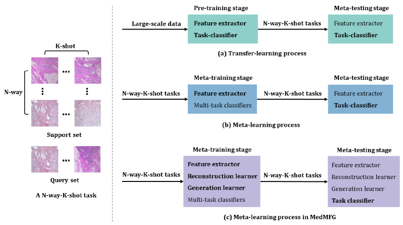
Specifically, there are two main differences between FSL and general classification. Firstly, the train set and test set in FSL have no overlapping classes. Specifically, FSL models are pretrained on the base dataset with base classes , and they need to predict novel classes on the novel dataset , where . Secondly, FSL utilizes a meta-task with the -way--shot approach during both the training and testing phases, as depicted in the left part of Fig. 1. In each meta-test ( meta-test), the support sets and the query set are randomly drawn from the . Specifically, categories are randomly selected from , and images per category are used as . Obviously, the limited availability of often leads to severe overfitting of the classifiers, causing difficulties in accurately predicting the categories of .
In few-shot medical image classification, we adhere to the setting rules of classical few-shot learning (FSL). Apart from this, there is a notable difference in our experiments, as the domain gap between and is more pronounced. For instance, in the CDFSL benchmark [2], comprises natural images, whereas consists of two different modalities of medical images. This larger modality and the semantic gap in few-shot medical image classification make it difficult for pre-trained models to accurately represent the target classes in medical images. The inaccurately represented features exacerbate distribution bias when handling new class distributions. Therefore, obtaining accurate feature representation through re-representation and acquiring precise class distribution from limited data are key to improving the performance of few-shot medical image classification.
III Related Work
III-A Transfer learning for FSL
Transfer learning-based methods [20, 3, 21] primarily aim to enhance the generalization ability of the representation model on cross-domain data. As illustrated in Fig. 1(a), these methods learn a universal image representation capability on the pre-training data . During the meta-testing phase, the feature extraction part of the model is typically frozen, and the classifier is trained online using , allowing predictions to be made on . Although transfer learning-based representation learning methods have been extensively researched and applied in traditional few-shot learning tasks, medical images present distinct challenges including diverse modalities, closer inter-class similarity, and the difficulty of directly transferring representation abilities from natural images. Consequently, our approach focuses on improving the performance of medical few-shot learning by directly increasing the number of training samples for medical target categories.
III-B Meta learning for FSL
Meta-learning-based methods [22, 23] strive to equip machines with the ability to learn how to learn. The objective is to achieve a universal classification capability through meta-training, enabling rapid adaptation to new tasks, as depicted in Fig. 1(b). During the training process, meta-learning methods iterate tasks using the same -way--shot setup as in testing. This iterative process results in a feature extractor that possesses robust generalization ability. Although meta-learning methods have shown promising performance in classical few-shot learning tasks, where they learn representation [24, 25, 26, 27], classification [28], or optimization [29], they often prove inadequate when faced with more complex domains like medicine and industry. Drawing inspiration from meta-learning approaches, we incorporate meta-training strategies, as in Fig. 1(c). Specifically, in each training episode, we deliberately define visible and unseen samples to augment the model’s capability to fully consider information from unseen samples and facilitate feature interactions.
IV Method
IV-A Method overview
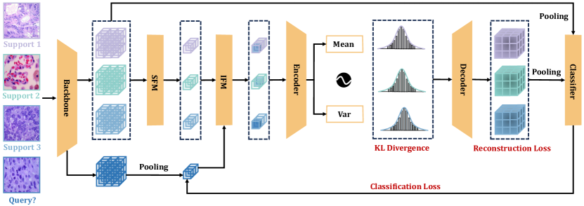
We propose MedMFG, as in Fig. 2, consisting of three modules: the self-construction feature module (SFM), the inter-construction feature module (IFM), and the variational sample generation module (VSGM). After feature extraction, SFM and IFM enhance the class characteristics of the prototype features. Then, VSGM can generate sufficient class-discriminative samples for each prototype. These augmented samples are trained together with the prototype features to improve the generalization ability and classification accuracy of the classifier. Clearly, the training and utilization of MedMFG are independent of the feature extraction backbone, meaning that MedMFG can flexibly and widely integrate with various backbones or existing representation learning methods.
During the training phase, MedMFG adopts a meta-training approach. A training set is sampled, with serving as the support set and as the query set. We follow exactly the same pre-training method as in other work to get the feature extraction backbone [30, 31]. Then, freezing the backbone, we train MedMFG using classification loss, KL divergence, and reconstruction loss.
In the meta-test phase, the backbone and MedMFG are both frozen. We only train classifiers online for each task. After feature extraction, SFM, and IFM, we obtain the support features with updated weights from the original support images, as well as the query features form the query image. Next, we generate new samples for each support feature by VSGM. In the -way--shot setup, we obtain -way- shot representative samples. Subsequently, we train the classifier using the generated new features along with the prototype features to classify .
IV-B Model structure and loss function
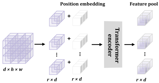
SFM: SFM increases the weight of category-specific information in prototype features through self-attention mechanisms. As depicted in Fig. 3, the support samples are fed into the embedding module , resulting in the prototype features , where denotes the number of channels, and and represent the height and width of the features, respectively. In SFM, the inputs are , where employs sinusoidal position encoding. The output of SFM is computed using the standard self-attention operation in the Transformer Encoder [32], performing multi-attention calculations using Eq. (1)
| (1) |
Thus, we obtain the re-characterized features as:
| (2) |
where are the learnable weights with size. Finally, is calculated continually by a layer normalization and an MLP.
| (3) |
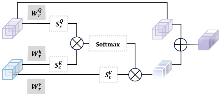
IFM: IFM enhances the weight of information related to the test samples in prototype features through interactive attention mechanisms. After we obtain the self-reconstructed feature of the support set, as well as the pooled query prototype feature , we construct the IFM module shown as Fig. 4 to embed the attention weights between and into the features of , resulting in the new support feature :
| (4) |
where follows Eq.(1). Therefore, in order to better learn the feature interaction capability of the IFM module, we adopt a meta-training approach to better simulate the embedding of unknown features with known features.
VSGM: VSGM utilizes an MLP-based VAE to perform variational augmentation on the input features and train a more generalized classifier. As in Fig. 2, the VAE consists of two parts: an encoder which map the input feature to a latent code , and a decoder , which reconstructs from , where and are weight parameters of and . Same as the traditional VAE [33], we approximate the true posterior distribution with another distribution . Thus, the KL scatter between the two distributions is:
| (5) |
Loss function: We design a three-part loss function to optimize MedMFG: the KL scatter, the reconstruction loss, and the classification loss. To diversify the samples generated by VSGM, we set the prior distribution of to a centered isotropic multivariate Gaussian: . For the posterior distribution, we assume it to be a multivariate Gaussian with diagonal covariance: . The KL divergence can be calculated by Eq. (5):
| (6) |
To drive VSGM to generate high-quality features, we design the reconstruction feature loss:
| (7) |
After obtaining augmented samples , for each meta-training task , we train an online classifier to predict the class of the query , resulting in a classification loss:
| (8) |
where refers to the true label of . The classification loss is crucial as it can help the SFM and IFM maintain the class properties when reconstructing features, and the features generated by VSGM do not deviate from the original category boundaries. Thus, the overall loss function is a weighted combination of the aforementioned terms:
| (9) |
The performance is experimentally verified to be optimal for and .
| Method | Backbone | miniImageNet ChestX | miniImageNet ISIC | ||||
|---|---|---|---|---|---|---|---|
| 5-shot | 20-shot | 50-shot | 5-shot | 20-shot | 50-shot | ||
| Baseline-1 [30] | Conv-4 | ||||||
| +MedMFG | Conv-4 | ||||||
| Baseline-1 [30] | ResNet-10 | ||||||
| +MedMFG | ResNet-10 | ||||||
| Baseline-1 [30] | ResNet-18 | ||||||
| +MedMFG | ResNet-18 | ||||||
| Baseline-2 [31] | ResNet-10 | ||||||
| +MedMFG | ResNet-10 | ||||||
| Baseline-3 [43] | ResNet-10 | ||||||
| +MedMFG | ResNet-10 | ||||||
V Experiments
V-A Experimental setup
Datasets: We validate our method on two benchmarks: CDFSL [2] and FHIST [44], following the standard few-shot setting as in previous works [45, 46, 3]. Specifically, on CDFSL, we regard miniImageNet [31], a dataset excerpted from ImageNet, as the base set while ISIC [47], a dermoscopic image dataset and chestX [48], a frontal-view X-ray images dataset as the novel set respectively. On FHIST, we train MedMFG on CRC-TP [49] (colorectal tissues images) and test it on LC25000 (colorectal and lung tissues images) [50], BreakHis (breast tissues images) [51], and NCT-CRC-HE-100k (colorectal tissues images) [52]. It is important to note that we follow the inductive setting, ensuring no information leakage among different queries.
Learnable parameters: MedMFG is designed to be lightweight and portable. Among the three modules, SFM consists of one transformer block with 1.66M parameters, IFM consists of another transformer block with 1.24M parameters, and the VAE module has 0.79M parameters. In total, MedMFG has 3.69M parameters. To ensure a fair comparison, we use the same feature extractor as the comparison methods.
Implementation details: During the meta-training phase, we follow the 5-way-1-shot approach for training. In the meta-testing phase, after extracting the features of support and novel data, we apply MedMFG to amplify each support feature into samples. We report the accuracy on standard N-way K-shot settings with query samples per class. All testing experiments are randomly sampled over 600 episodes. The learning rate of MedMFG is set to 0.00001, and it is optimized with Adam.
V-B Result analysis
Comparison to state-of-the-Art (SOTA) methods: We compare our method with the SOTA methods on CDFSL and FHIST benchmarks. On FHIST, as shown in Tab. I, MedMFG achieves the new state-of-the-art in all three migration settings. For instance, on CRC-TP NCT, MedMFG outperforms Finetune [37] by , , and on 5-way 1-shot, 5-shot, and 10-shot settings, respectively. In other scenarios like CRC-TP LC25000 and CRC-TP BreakHis, our method surpasses the current optimal results by , , , , , and . It is worth noting that Finetune [37] requires retraining during testing, whereas our approach is completely frozen during testing without any additional consumption of time and space. These results demonstrate the superiority and practicality of MedMFG in a wide range of medical domain migrations.
On CDFSL, as shown in Tab. II, MedMFG achieves a new SOTA on most of the results. For example, on miniImageNetChestX and ISIC, MedMFG outperforms ConFess [40] by , , , and on 5-way 5-shot and 20-shot settings. In the 50-shot setting, our method reaches the current optimum. These results highlight the strong generalization ability of MedMFG.
In summary, whether it involves cross-domain transfer from natural images to medical images or cross-category transfer on medical images, MedMFG demonstrates stronger generalization capabilities. This proves the effectiveness of the feature design and augmentation methods in medical images, providing a novel approach to address the challenges posed by the limited availability of medical data.
Fusion experiments: To demonstrate the generalizability and flexibility of our method, we extract features using multiple backbones and baselines, and then fuse MedMFG amplification samples. As shown in Tab. III, we validate the fusion results of MedMFG with three feature extractors, Conv-4 [53], ResNet-10 [54], and ResNet-18 [54], as well as three methods [30, 31, 43]. MedMFG consistently improves the performance by more than 2.9% across all settings. Particularly, it surpasses the baseline by 6% in the two results with ResNet-18. Notably, it exhibits superior performance even with fewer support instances, indicating that the generated feature samples accurately capture class characteristics. These results highlight the versatility of MedMFG, which is not restricted to specific datasets or feature extractors. As a result, various works based on different backbones can benefit from our approach.
| Method | SFM | IFM | Layers | CRC-TP NCT | ||
|---|---|---|---|---|---|---|
| 1-shot | 5-shot | 10-shot | ||||
| Baseline [30] | 58.1 | 72.3 | 74.4 | |||
| MedMFG-1 | 58.7 | 73.6 | 75.7 | |||
| MedMFG-2 | 59.0 | 75.3 | 79.0 | |||
| MedMFG-3 | one | 67.3 | 84.0 | 84.3 | ||
| MedMFG-4 | two | 63.1 | 77.0 | 76.3 | ||
| MedMFG-5 | two | 66.5 | 83.9 | 83.7 | ||
| MedMFG-6 | three | 69.0 | 85.7 | 86.9 | ||
| MedMFG-7 | two | 60.0 | 75.6 | 76.1 | ||
| MedMFG | two | 69.2 | 85.2 | 87.7 | ||
Ablation studies: In Tab. IV, we analyze the effectiveness of the three modules in MedMFG: SFM, IFM, and VSGM. Additionally, we compare the performance with varying numbers of layers in the VAE. The results show that using SFM or IFM alone does not lead to significant improvements, especially in the 1-shot setting. This is because, without the feature augmentation module, a single sample fails to adequately represent the entire distribution of a class, resulting in a substantial bias. However, the last three rows clearly demonstrate the crucial role of SFM and IFM in conjunction with feature augmentation. The absence of SFM or IFM results in a performance decrease of more than 2.5%. This indicates that feature reconstruction effectively highlights class characteristics and reduces intra-class distances, contributing to improved performance. Moreover, when comparing MedMFG-3 with MedMFG, it can be observed that the VAE with a two-layer MLP structure better simulates the characteristics of real samples. However, blindly increasing the number of MLP layers provides minimal benefits while adding more parameters and increasing training complexity. Additionally, in the 20-shot setting, MedMFG-6 performs worse than MedMFG, suggesting that excessive feature expression can limit feature diversity. Therefore, we ultimately choose the VAE composed of a two-layer MLP as the final structure.
V-C Visualization
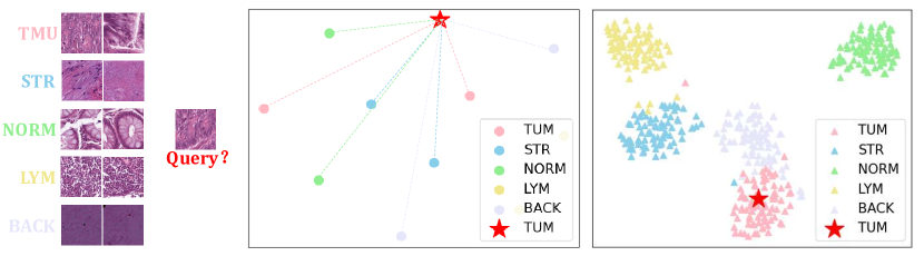
We assert that MedMFG is capable of generating representative samples to enhance classification results. To visualize this, we present the original features generated by the feature extractor and the augmented features of MedMFG on the NCT dataset in Fig. 5. In this example, the true label of the query is TMU. However, due to the fine-grained nature of the support classes, the difference in distance between the query and each support feature is small, resulting in overfitting of the linear regression classifier and misclassification errors. Nevertheless, after variational feature generation by MedMFG to adjust the distribution, the query is accurately included within the distribution boundary of TMU.
VI Conclusion
Summary: In this paper, to enhance the generalization ability of the classifier in few-shot medical image classification, we propose MedMFG. It is a plug-and-play method that can augment sufficient class-discriminative features from a small number of samples. Through comparison experiments, we demonstrate the superiority of our method by achieving new SOTA in multiple benchmarks. Furthermore, fusion experiments showcase the flexibility and applicability of our method.
Limitations: By comparing the baseline with MedMFG-1, as well as MedMFG-4 and MedMFG-7 in Tab. IV, it is apparent that employing the self-attention mechanism alone yields limited improvement over the baseline. In contrast, when combined with VSGM, the self-attention mechanism demonstrates promising performance. The cross-attention mechanism exhibits similar characteristics. We will investigate the generalizability of this phenomenon through additional experiments. Furthermore, we aim to explore additional medical modalities like CT and MRI, enhancing the practicality of MedMFG.
References
- [1] Y. Wang, Q. Yao, J. T. Kwok, and L. M. Ni, “Generalizing from a few examples: A survey on few-shot learning,” ACM computing surveys (csur), vol. 53, no. 3, pp. 1–34, 2020.
- [2] Y. Guo, N. C. Codella, L. Karlinsky, J. V. Codella, J. R. Smith, K. Saenko, T. Rosing, and R. Feris, “A broader study of cross-domain few-shot learning,” in European conference on computer vision. Springer, 2020, pp. 124–141.
- [3] Q. Guo, G. Haotong, X. Wei, Y. Fu, Y. Yu, W. Zhang, and W. Ge, “Rankdnn: Learning to rank for few-shot learning,” in Proceedings of the AAAI Conference on Artificial Intelligence, vol. 37, no. 1, 2023, pp. 728–736.
- [4] Z. Dai, J. Yi, L. Yan, Q. Xu, L. Hu, Q. Zhang, J. Li, and G. Wang, “Pfemed: Few-shot medical image classification using prior guided feature enhancement,” Pattern Recognition, vol. 134, p. 109108, 2023.
- [5] A. Paul, Y.-X. Tang, T. C. Shen, and R. M. Summers, “Discriminative ensemble learning for few-shot chest x-ray diagnosis,” Medical image analysis, vol. 68, p. 101911, 2021.
- [6] M. Yazdanpanah and P. Moradi, “Visual domain bridge: A source-free domain adaptation for cross-domain few-shot learning,” in Proceedings of the IEEE/CVF Conference on Computer Vision and Pattern Recognition, 2022, pp. 2868–2877.
- [7] Y. He, W. Liang, D. Zhao, H. Zhou, W. Ge, Y. Yu, and W. Zhang, “Attribute surrogates learning and spectral tokens pooling in transformers for few-shot learning,” in IEEE/CVF Conference on Computer Vision and Pattern Recognition, CVPR 2022, New Orleans, LA, USA, June 18-24, 2022. IEEE, 2022, pp. 9109–9119.
- [8] H. Jiang, M. Gao, H. Li, R. Jin, H. Miao, and J. Liu, “Multi-learner based deep meta-learning for few-shot medical image classification,” IEEE Journal of Biomedical and Health Informatics, vol. 27, no. 1, pp. 17–28, 2022.
- [9] R. Singh, V. Bharti, V. Purohit, A. Kumar, A. K. Singh, and S. K. Singh, “Metamed: Few-shot medical image classification using gradient-based meta-learning,” Pattern Recognition, vol. 120, p. 108111, 2021.
- [10] V.-K. Vo-Ho, K. Yamazaki, H. Hoang, M.-T. Tran, and N. Le, “Meta-learning of nas for few-shot learning in medical image applications,” arXiv preprint arXiv:2203.08951, 2022.
- [11] P. Khandelwal and P. Yushkevich, “Domain generalizer: A few-shot meta learning framework for domain generalization in medical imaging,” in Domain Adaptation and Representation Transfer, and Distributed and Collaborative Learning. Springer, 2020, pp. 73–84.
- [12] S. Foti, B. Koo, D. Stoyanov, and M. J. Clarkson, “3d shape variational autoencoder latent disentanglement via mini-batch feature swapping for bodies and faces,” in IEEE/CVF Conference on Computer Vision and Pattern Recognition, CVPR 2022, New Orleans, LA, USA, June 18-24, 2022. IEEE, 2022, pp. 18 709–18 718.
- [13] D. Danks and C. Yau, “Basisdevae: Interpretable simultaneous dimensionality reduction and feature-level clustering with derivative-based variational autoencoders,” in Proceedings of the 38th International Conference on Machine Learning, ICML 2021, 18-24 July 2021, Virtual Event, ser. Proceedings of Machine Learning Research, M. Meila and T. Zhang, Eds., vol. 139. PMLR, 2021, pp. 2410–2420.
- [14] H. Zhao, J. Jia, and V. Koltun, “Exploring self-attention for image recognition,” in Proceedings of the IEEE/CVF conference on computer vision and pattern recognition, 2020, pp. 10 076–10 085.
- [15] A. Vaswani, N. Shazeer, N. Parmar, J. Uszkoreit, L. Jones, A. N. Gomez, Ł. Kaiser, and I. Polosukhin, “Attention is all you need,” Advances in neural information processing systems, vol. 30, 2017.
- [16] J. Lu, P. Gong, J. Ye, J. Zhang, and C. Zhang, “A survey on machine learning from few samples,” Pattern Recognit., vol. 139, p. 109480, 2023.
- [17] L. Tang, D. Wertheimer, and B. Hariharan, “Revisiting pose-normalization for fine-grained few-shot recognition,” in Proceedings of the IEEE/CVF conference on computer vision and pattern recognition, 2020, pp. 14 352–14 361.
- [18] Y. Cao, W. Zhu, J. Yang, G. Fu, D. Lin, and Y. Cao, “An effective industrial defect classification method under the few-shot setting via two-stream training,” Optics and Lasers in Engineering, vol. 161, p. 107294, 2023.
- [19] H. Tang, X. Liu, S. Sun, X. Yan, and X. Xie, “Recurrent mask refinement for few-shot medical image segmentation,” in Proceedings of the IEEE/CVF international conference on computer vision, 2021, pp. 3918–3928.
- [20] M. N. Rizve, S. Khan, F. S. Khan, and M. Shah, “Exploring complementary strengths of invariant and equivariant representations for few-shot learning,” in Proceedings of the IEEE/CVF conference on computer vision and pattern recognition, 2021, pp. 10 836–10 846.
- [21] W.-Y. Chen, Y.-C. Liu, Z. Kira, Y.-C. F. Wang, and J.-B. Huang, “A closer look at few-shot classification,” arXiv preprint arXiv:1904.04232, 2019.
- [22] C. Finn, P. Abbeel, and S. Levine, “Model-agnostic meta-learning for fast adaptation of deep networks,” in International conference on machine learning. PMLR, 2017, pp. 1126–1135.
- [23] A. Nichol and J. Schulman, “Reptile: a scalable metalearning algorithm,” arXiv preprint arXiv:1803.02999, vol. 2, no. 3, p. 4, 2018.
- [24] A. Nichol, J. Achiam, and J. Schulman, “On first-order meta-learning algorithms,” CoRR, vol. abs/1803.02999, 2018.
- [25] A. Antoniou, H. Edwards, and A. J. Storkey, “How to train your MAML,” in 7th International Conference on Learning Representations, ICLR 2019, New Orleans, LA, USA, May 6-9, 2019. OpenReview.net, 2019.
- [26] X. Song, W. Gao, Y. Yang, K. Choromanski, A. Pacchiano, and Y. Tang, “ES-MAML: simple hessian-free meta learning,” in 8th International Conference on Learning Representations, ICLR 2020, Addis Ababa, Ethiopia, April 26-30, 2020. OpenReview.net, 2020.
- [27] L. Collins, A. Mokhtari, S. Oh, and S. Shakkottai, “MAML and ANIL provably learn representations,” in International Conference on Machine Learning, ICML 2022, 17-23 July 2022, Baltimore, Maryland, USA, ser. Proceedings of Machine Learning Research, K. Chaudhuri, S. Jegelka, L. Song, C. Szepesvári, G. Niu, and S. Sabato, Eds., vol. 162. PMLR, 2022, pp. 4238–4310.
- [28] C. Kao, W. Chiu, and P. Chen, “MAML is a noisy contrastive learner in classification,” in The Tenth International Conference on Learning Representations, ICLR 2022, Virtual Event, April 25-29, 2022. OpenReview.net, 2022.
- [29] M. Andrychowicz, M. Denil, S. G. Colmenarejo, M. W. Hoffman, D. Pfau, T. Schaul, and N. de Freitas, “Learning to learn by gradient descent by gradient descent,” in Advances in Neural Information Processing Systems 29: Annual Conference on Neural Information Processing Systems 2016, December 5-10, 2016, Barcelona, Spain, D. D. Lee, M. Sugiyama, U. von Luxburg, I. Guyon, and R. Garnett, Eds., 2016, pp. 3981–3989.
- [30] J. Snell, K. Swersky, and R. S. Zemel, “Prototypical networks for few-shot learning,” in Advances in Neural Information Processing Systems 30: Annual Conference on Neural Information Processing Systems 2017, December 4-9, 2017, Long Beach, CA, USA, I. Guyon, U. von Luxburg, S. Bengio, H. M. Wallach, R. Fergus, S. V. N. Vishwanathan, and R. Garnett, Eds., 2017, pp. 4077–4087.
- [31] O. Vinyals, C. Blundell, T. Lillicrap, K. Kavukcuoglu, and D. Wierstra, “Matching networks for one shot learning,” in Advances in Neural Information Processing Systems 29: Annual Conference on Neural Information Processing Systems 2016, December 5-10, 2016, Barcelona, Spain, D. D. Lee, M. Sugiyama, U. von Luxburg, I. Guyon, and R. Garnett, Eds., 2016, pp. 3630–3638.
- [32] A. Dosovitskiy, L. Beyer, A. Kolesnikov, D. Weissenborn, X. Zhai, T. Unterthiner, M. Dehghani, M. Minderer, G. Heigold, S. Gelly et al., “An image is worth 16x16 words: Transformers for image recognition at scale,” arXiv preprint arXiv:2010.11929, 2020.
- [33] D. P. Kingma and M. Welling, “Auto-encoding variational bayes,” in 2nd International Conference on Learning Representations, ICLR 2014, Banff, AB, Canada, April 14-16, 2014, Conference Track Proceedings, Y. Bengio and Y. LeCun, Eds., 2014.
- [34] K. Lee, S. Maji, A. Ravichandran, and S. Soatto, “Meta-learning with differentiable convex optimization,” arXiv e-prints, 2019.
- [35] Y. Wang, W. Chao, K. Q. Weinberger, and L. van der Maaten, “Simpleshot: Revisiting nearest-neighbor classification for few-shot learning,” CoRR, vol. abs/1911.04623, 2019.
- [36] Y. Tian, Y. Wang, D. Krishnan, J. B. Tenenbaum, and P. Isola, “Rethinking few-shot image classification: A good embedding is all you need?” in Computer Vision - ECCV 2020 - 16th European Conference, Glasgow, UK, August 23-28, 2020, Proceedings, Part XIV, ser. Lecture Notes in Computer Science, A. Vedaldi, H. Bischof, T. Brox, and J. Frahm, Eds., vol. 12359. Springer, 2020, pp. 266–282.
- [37] W. Y. Chen, Y. C. Liu, Z. Kira, Y. Wang, and J. B. Huang, “A closer look at few-shot classification,” in arXiv, 2019.
- [38] H.-Y. Tseng, H.-Y. Lee, J.-B. Huang, and M.-H. Yang, “Cross-domain few-shot classification via learned feature-wise transformation,” arXiv preprint arXiv:2001.08735, 2020.
- [39] H. Wang and Z.-H. Deng, “Cross-domain few-shot classification via adversarial task augmentation,” arXiv preprint arXiv:2104.14385, 2021.
- [40] D. Das, S. Yun, and F. Porikli, “Confess: A framework for single source cross-domain few-shot learning,” in International Conference on Learning Representations, 2022.
- [41] Y. Hu and A. J. Ma, “Adversarial feature augmentation for cross-domain few-shot classification,” in Computer Vision–ECCV 2022: 17th European Conference, Tel Aviv, Israel, October 23–27, 2022, Proceedings, Part XX. Springer, 2022, pp. 20–37.
- [42] P. Li, S. Gong, C. Wang, and Y. Fu, “Ranking distance calibration for cross-domain few-shot learning,” in Proceedings of the IEEE/CVF Conference on Computer Vision and Pattern Recognition, 2022, pp. 9099–9108.
- [43] F. Sung, Y. Yang, L. Zhang, T. Xiang, P. H. S. Torr, and T. M. Hospedales, “Learning to compare: Relation network for few-shot learning,” in 2018 IEEE Conference on Computer Vision and Pattern Recognition, CVPR 2018, Salt Lake City, UT, USA, June 18-22, 2018. Computer Vision Foundation / IEEE Computer Society, 2018, pp. 1199–1208.
- [44] F. Shakeri, M. Boudiaf, S. Mohammadi, I. Sheth, M. Havaei, I. B. Ayed, and S. E. Kahou, “Fhist: A benchmark for few-shot classification of histological images,” arXiv preprint arXiv:2206.00092, 2022.
- [45] A. Parnami and M. Lee, “Learning from few examples: A summary of approaches to few-shot learning,” arXiv preprint arXiv:2203.04291, 2022.
- [46] Y. He, W. Liang, D. Zhao, H.-Y. Zhou, W. Ge, Y. Yu, and W. Zhang, “Attribute surrogates learning and spectral tokens pooling in transformers for few-shot learning,” in Proceedings of the IEEE/CVF Conference on Computer Vision and Pattern Recognition, 2022, pp. 9119–9129.
- [47] P. Tschandl, C. Rosendahl, and H. Kittler, “The ham10000 dataset, a large collection of multi-source dermatoscopic images of common pigmented skin lesions,” Scientific data, vol. 5, no. 1, pp. 1–9, 2018.
- [48] X. Wang, Y. Peng, L. Lu, Z. Lu, M. Bagheri, and R. M. Summers, “Chestx-ray8: Hospital-scale chest x-ray database and benchmarks on weakly-supervised classification and localization of common thorax diseases,” in Proceedings of the IEEE conference on computer vision and pattern recognition, 2017, pp. 2097–2106.
- [49] S. Javed, A. Mahmood, N. Werghi, K. Benes, and N. Rajpoot, “Multiplex cellular communities in multi-gigapixel colorectal cancer histology images for tissue phenotyping,” IEEE Transactions on Image Processing, vol. 29, pp. 9204–9219, 2020.
- [50] A. A. Borkowski, M. M. Bui, L. B. Thomas, C. P. Wilson, L. A. DeLand, and S. M. Mastorides, “Lung and colon cancer histopathological image dataset (lc25000),” arXiv preprint arXiv:1912.12142, 2019.
- [51] F. A. Spanhol, L. S. Oliveira, C. Petitjean, and L. Heutte, “A dataset for breast cancer histopathological image classification,” Ieee transactions on biomedical engineering, vol. 63, no. 7, pp. 1455–1462, 2015.
- [52] B. Á. Pataki, A. Olar, D. Ribli, A. Pesti, E. Kontsek, B. Gyöngyösi, Á. Bilecz, T. Kovács, K. A. Kovács, Z. Kramer et al., “Huncrc: annotated pathological slides to enhance deep learning applications in colorectal cancer screening,” Scientific Data, vol. 9, no. 1, p. 370, 2022.
- [53] A. Krizhevsky, I. Sutskever, and G. E. Hinton, “Imagenet classification with deep convolutional neural networks,” in Advances in Neural Information Processing Systems 25: 26th Annual Conference on Neural Information Processing Systems 2012. Proceedings of a meeting held December 3-6, 2012, Lake Tahoe, Nevada, United States, P. L. Bartlett, F. C. N. Pereira, C. J. C. Burges, L. Bottou, and K. Q. Weinberger, Eds., 2012, pp. 1106–1114.
- [54] K. He, X. Zhang, S. Ren, and J. Sun, “Deep residual learning for image recognition,” in 2016 IEEE Conference on Computer Vision and Pattern Recognition, CVPR 2016, Las Vegas, NV, USA, June 27-30, 2016. IEEE Computer Society, 2016, pp. 770–778.