Structure-Aware Analyses and Algorithms for Interpolative Decompositions

Abstract

Low-rank approximation is a task of critical importance in modern science, engineering, and statistics. Many low-rank approximation algorithms, such as the randomized singular value decomposition (RSVD), project their input matrix into a subspace approximating the span of its leading singular vectors. Other algorithms compress their input into a small subset of representative rows or columns, leading to a so-called interpolative decomposition. This paper investigates how the accuracy of interpolative decompositions is affected by the structural properties of the input matrix being operated on, including how these properties affect the performance comparison between interpolative decompositions and RSVD. We also introduce a novel method of interpolative decomposition in the form of the randomized Golub-Klema-Stewart (RGKS) algorithm, which combines RSVD with a pivoting strategy for column subset selection. Through numerical experiments, we find that matrix structures including singular subspace geometry and singular spectrum decay play a significant role in determining the performance comparison between these different algorithms. We also prove inequalities which bound the error of a general interpolative decomposition in terms of these matrix structures. Lastly, we develop forms of these bounds specialized to RGKS while considering how randomization affects the approximation error of this algorithm.

65F55, 68W20

1 Introduction

Countless numerical algorithms in science, engineering, and statistics are built upon linear-algebraic primitives such as matrix multiplication, eigen-decomposition, linear system solvers, and linear least-squares solvers. Unfortunately, the classical algorithms for these tasks generally have cubically scaling runtimes, making them ill-suited for the extremely large matrices arising in modern applications. Low-rank approximations of large matrices provide a means to efficiently perform computations which would otherwise be prohibitively expensive. A low-rank approximation of an $m\times n$ matrix ${\mathbf{A}}$ is a decomposition

$${\mathbf{A}}\approx{\mathbf{B}}_{1}{\mathbf{B}}_{2}^{\mathrm{T}},$$

where ${\mathbf{B}}_{1}$ is $m\times k$, ${\mathbf{B}}_{2}$ is $n\times k$, and $k\ll\min\{m,\,n\}$. We can refer to this more specifically as a rank-$k$ approximation. The key property of this approximation is that the dimensions of ${\mathbf{B}}_{1}$ and ${\mathbf{B}}_{2}$ are much smaller than those of ${\mathbf{A}}$, meaning that by working with ${\mathbf{B}}_{1}$ and ${\mathbf{B}}_{2}$ instead of with ${\mathbf{A}}$ directly, basic computations can be performed more efficiently.

Many algorithms for computing a rank-$k$ approximation fall into two broad categories. In the first category are algorithms that identify a “structurally important” $k$-dimensional subspace ${\mathcal{Q}}\subseteq{\mathbb{R}}^{m}$, represented by an orthonormal basis ${\mathbf{Q}}\in{\mathbb{R}}^{m\times k}$ whose columns are estimates of the leading left singular vectors of ${\mathbf{A}}$— leading to the low-rank approximation ${\mathbf{B}}_{1}={\mathbf{Q}},\,{\mathbf{B}}_{2}={\mathbf{A}}^{\mathrm{T}}{\mathbf{Q}}$. Algorithms in this category include randomized SVD, subspace iteration, and block-Krylov methods [19, 26, 31]. We will focus primarily on the randomized SVD (RSVD). The second category encompasses so-called interpolative decompositions, which identify a small subset of indices $J=\{j_{1},\,\ldots,\,j_{k}\}$ corresponding to the most “structurally important” rows or columns. In the case where $J$ is a set of column indices, this leads to a low-rank approximation ${\mathbf{B}}_{1}={\mathbf{A}}_{:,\,J},\,{\mathbf{B}}_{2}^{\mathrm{T}}=({\mathbf{A}}_{:,\,J})^{\dagger}{\mathbf{A}}$, where the subscript “$:,\,J$” is Matlab notation for selecting a column subset, and $\dagger$ denotes the Moore-Penrose pseudoinverse. The columns in $J$ (represented exactly in the approximation) are sometimes called the “skeleton columns.” Approximations which use row indices, or row and column indices simultaneously (e.g., CUR and pseudo-skeleton decompositions), can be constructed in a way that is essentially equivalent. This paper will therefore focus on approximations based on column selection. Minimizing the approximation error over all choices of $k$ skeleton columns is NP hard [13, 35], but a variety of algorithms exist for choosing approximately optimal columns. These include approaches based on pivoted QR or LU factorizations [5, 6, 18, 21, 23, 28, 33], random column sampling strategies [10, 11, 13, 15, 24], and most importantly for this paper, selection strategies based on the singular value decomposition [13, 16, 24, 28].

While the RSVD can, in theory, project its input onto a subspace that includes the leading singular vectors, interpolative decompositions are more restricted in their choice of subspace—they must project their input into the span of a small column subset. This means that, with the exception of matrices having specially structured columns, interpolative decompositions cannot obtain optimal approximation error. In light of this handicap, it has traditionally been thought that algorithms such as RSVD, which explicitly estimate the leading singular vectors, are more accurate than interpolative decompositions. In practice, the situation is not so clear cut; for certain approximation ranks where accurate singular vector estimates are difficult to obtain, interpolative decompositions can have competitive accuracy to the RSVD, particularly if power iteration is not employed. To illustrate this point, we refer to Fig. 1, which plots the relative approximation error of three randomized low-rank approximation algorithms as a function of the approximation rank. One of these algorithms is the RSVD, and the other two are interpolative decompositions: RID, which selects columns using a rank-revealing QR factorization on a random Gaussian embedding of the input matrix [23, 33], and RGKS, a novel procedure we introduce in this paper. An important feature of Fig. 1 is that the RID and RGKS have accuracy which is competitive with RSVD when power iteration is not used. This comparison places all three algorithms on a similar footing in terms of the manner in which they access the input matrix. To be specific, each algorithm computes their approximation based on a small number of matrix-vector products with ${\mathbf{A}}$ or ${\mathbf{A}}^{\mathrm{T}}$, depending on the approximation rank $k$ and the oversampling parameter $p$. When RSVD is run without power iteration in Fig. 1, all three algorithms use an equal of matrix-vector products with the input matrix; RID uses $2(k+p)$ matrix-vector products with ${\mathbf{A}}^{\mathrm{T}}$, while RSVD and RGKS use $k+p$ matrix-vector products with ${\mathbf{A}}^{\mathrm{T}}$ and an additional $k+p$ with ${\mathbf{A}}$.

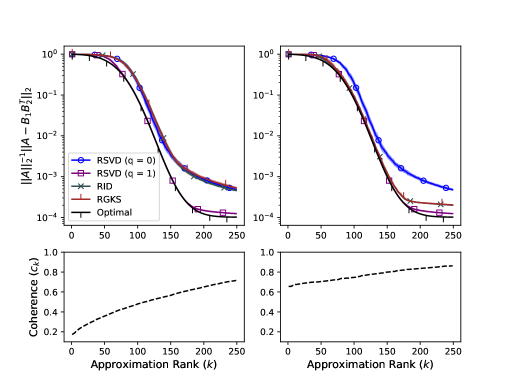
Figure 1: Relative spectral error $\|{\mathbf{A}}\|_{2}^{-1}\|{\mathbf{A}}-{\mathbf{B}}_{1}{\mathbf{B}}_{2}^{\mathrm{T}}\|_{2}$ for approximations computed by RID, RGKS, RSVD without power iteration $(q=0)$, and RSVD with one step of power iteration $(q=1)$, on two different square matrices of dimension $n=512$. The two matrices, corresponding to the left and right columns, differed in terms of the right singular subspaces’ coherence. All instances of RSVD, including those internal to RGKS, were computed with oversampling $p=\lceil k/10\rceil$ and then optimally reduced to rank $k$. To equalize the number of matrix-vector products, RID was run using a sketching matrix with $\min\{n,\,2(k+p)\}$ rows. Each curve shows the mean error over 100 approximations of the same matrix, with shaded regions indicating 10% and 90% error quantiles. Note that while RGKS and RID are strongly affected by differences in coherence, RSVD is completely unaffected, which is to be expected from the orthogonal invariance properties of a Gaussian sketch.

Beyond simply highlighting that interpolative decompositions can be competitive with RSVD given a fixed budget of matrix-vector products, this paper seeks to characterize the specific structures of the input matrix which affect the performance comparison between algorithms. Interpolative decompositions are already known to produce more structured and interpretable approximations than the RSVD [24], but we will focus rather on performance in the sense of approximation accuracy. The structures affecting approximation accuracy which we examine can be categorized into two groups: those which characterize the decay of a matrix’s singular spectrum, and those which characterize the geometry of its singular subspaces. For spectral decay, we will focus on the singular value gap and residual stable rank, defined by

$$\gamma_{k}=\frac{\sigma_{k+1}}{\sigma_{k}}\quad\text{and}\quad r_{k}=\sum_{i=k+1}^{\min\{m,\,n\}}\frac{\sigma_{i}^{2}}{\sigma_{k+1}^{2}},$$

where $\sigma_{1}\geq\ldots\geq\sigma_{\min\{m,\,n\}}\geq 0$ are the singular values of ${\mathbf{A}}$. The singular value gap has a long history in numerical linear algebra, playing a central role in the analysis of eigenvalue and singular value decomposition algorithms [17, 30], perturbation theory for invariant subspaces [8, 29, 32], and randomized singular vector estimation [27]. The stable rank of a matrix (defined as the squared ratio of its Frobenius norm over its spectral norm) has long been used as proxy for the true rank since, unlike true rank, it a continuous function of the matrix itself. The residual stable rank $r_{k}$ is a somewhat more recent concept, and has appeared in error analyses of algorithms including the RSVD [19] and determinental point processes [9].

To describe the geometry of a matrix’s singular subspaces, and the effects of this geometry on interpolative decomposition accuracy, we will use several concepts related to the singular value decomposition ${\mathbf{A}}={\mathbf{U}}{\mathbf{\Sigma}}{\mathbf{V}}^{\mathrm{T}}$. The central quantity of interest in this context is $\sigma_{\mathrm{min}}({\mathbf{V}}_{J,\,1:k})$, where $J$ is the set of skeleton column indices. Many results connecting $\sigma_{\mathrm{min}}({\mathbf{V}}_{J,\,1:k})$ to interpolative decomposition accuracy have appeared in the literature before; for example, it is known that

(1) $$\|{\mathbf{A}}-{\mathbf{A}}_{:,\,J}({\mathbf{A}}_{:,\,J})^{\dagger}{\mathbf{A}}\|_{2}\leq\frac{\sigma_{k+1}({\mathbf{A}})}{\sigma_{\mathrm{min}}({\mathbf{V}}_{J,\,1:k})}\quad\text{and}\quad\sin\phi_{\mathrm{max}}\leq\frac{\gamma_{k}}{\sigma_{\mathrm{min}}({\mathbf{V}}_{J,\,1:k})},$$

where $\phi_{\mathrm{max}}$ is the largest principal angle between $\operatorname{range}({\mathbf{A}}_{:,\,J})$ and $\operatorname{range}({\mathbf{U}}_{:,\,1:k})$. These inequalities arise from [21, Theorem 1.5] and [16, Theorems 3.1, 6.1], respectively. This paper will examine geometric properties of a matrix’s singular subspaces which affect the value of $\sigma_{\mathrm{min}}({\mathbf{V}}_{J,\,1:k})$. Particular focus will be given to the coherence of the leading singular subspace, defined as $c_{k}=\max_{1\leq j\leq n}\|{\mathbf{V}}_{j,\,1:k}\|_{2}$, which measures the concentration of its leverage score distribution. We will also find, in Section 6 and Section 7, that assigning a geometric interpretation to $\sigma_{\mathrm{min}}({\mathbf{V}}_{J,\,1:k})$ itself allows for several different error bounds to be presented in a unified notation, and simplifies the analysis of randomization errors in the RGKS algorithm (introduced below). Our focus on coherence is not without precedent; for example, it appears in the theory of matrix completion [2, 3], as well as in the analysis of differentially private low-rank approximation algorithms [20]. The graphs in Fig. 1 differ in terms of the coherence of the input matrix’s right singular subspaces, and from this figure, we see that coherence strongly affects the performance of the two interpolative decompositions.

Related to our structural analysis of interpolative decompositions, this paper also introduces the randomized Golub-Klema-Stewart algorithm, or RGKS. This is a randomized variant of the Golub-Klema-Stewart algorithm [16], an interpolative decomposition named for the authors who first introduced it in 1976. At a high level, RGKS selects skeleton columns by applying a rank-revealing QR factorization to a matrix of right singular vector estimates computed by the RSVD. Because RGKS operates directly on an estimate of the right singular subspace, it serves as a natural case study on the effects of subspace structures. Furthermore, because the subspace estimate is computed using RSVD, an algorithm whose accuracy is known to depend on structures in the singular spectrum, it will be natural to consider how the spectral and subspace effects couple with one another. In particular, prior work analyzes RSVD subspace estimates, e.g., [12, 27, 34], and this raises interesting possibilities for exploring how the particular subspace errors committed by RSVD interact with the subspace-dependent QR factorization in RGKS.

While RGKS serves as an “archetypal” interpolative decomposition to motivate our analysis of interpolative decompositions in general, we will also consider several interesting features which are unique to RGKS. Specifically, we will show that RGKS has attractive properties in terms of efficiency, accuracy, and robustness to noise arising from its internal randomization. We will also show that in many cases, RGKS produces more accurate approximations than leverage score sampling, a randomized interpolative decomposition algorithm which is similar to RGKS in its design.

2 Main Contributions

The main algorithmic contribution of this paper is RGKS, a sketching-based interpolative decomposition which combines a randomized SVD with a rank-revealing QR factorization. Section 4 describes this algorithm, and discusses its accuracy and efficiency in comparison to other interpolative decomposition algorithms. Section 7 develops error bounds for RGKS, and shows that the accuracy of RGKS is surprisingly robust to singular vector estimation errors arising from randomization.

The analytical contributions of this paper include error bounds that characterize how the structural properties of an input matrix affect the accuracy of interpolative decompositions. In stating these bounds, ${\mathbf{\Sigma}}_{\perp}=\mathrm{diag}(\sigma_{i}\,:\,i\geq k+1)$ denotes the matrix of trailing singular values of ${\mathbf{A}}$, so that $\|{\mathbf{\Sigma}}_{\perp}\|$ is the optimal approximation error in the spectral or Frobenius norm. The span of the first $k$ right singular vectors of ${\mathbf{A}}$ is denoted by ${\mathcal{V}}_{k}$, and to ensure that this subspace is well defined, we assume that $\sigma_{k}({\mathbf{A}})>\sigma_{k+1}({\mathbf{A}})$. As is customary, ${\mathbf{e}}_{j}$ denotes the $j{{}^{\text{th}}}$ elementary unit vector. We now summarize our main error bounds in the theorem below, which is a concatenation of Theorems 6.1, 6.5 and 6.7.

Theorem 2.1.

Choose $k\leq n/2$ such that $\sigma_{k}({\mathbf{A}})>\sigma_{k+1}({\mathbf{A}})$. Given a set of skeleton column indices $J\subseteq\{1,\,\ldots,\,n\}$ with $|J|=k$, define the approximation error ${\mathbf{E}}={\mathbf{A}}-{\mathbf{A}}_{:,\,J}({\mathbf{A}}_{:,\,J})^{\dagger}{\mathbf{A}}$, and let $\varphi_{1},\,\ldots,\,\varphi_{k}\in[0,\,\pi/2]$ be the principal angles between ${\mathcal{V}}_{k}$ and ${\mathcal{I}}_{J}\mathrel{\hbox to0.0pt{\raisebox{1.29167pt}{$\cdot$}\hss}\raisebox{-1.29167pt}{$\cdot$}}=\operatorname{span}\{{\mathbf{e}}_{j}\,:\,j\in J\}$. If $\max_{1\leq i\leq n}\varphi_{i}<\pi/2$, then

(2) $$\|{\mathbf{E}}\|_{2}\leq\|{\mathbf{\Sigma}}_{\perp}\|_{2}\sec({\textstyle\max_{1\leq i\leq k}\varphi_{i}})\quad\text{and}\quad\|{\mathbf{E}}\|_{\mathrm{F}}\leq\|{\mathbf{\Sigma}}_{\perp}\|_{\mathrm{F}}\sqrt{1+\frac{1}{r_{k}}\sum_{i=1}^{k}\tan^{2}\varphi_{i}},$$

where $r_{k}=\|{\mathbf{\Sigma}}_{\perp}\|_{\mathrm{F}}^{2}/\|{\mathbf{\Sigma}}_{\perp}\|_{2}^{2}$ is the residual stable rank. If $\sigma_{k+1}({\mathbf{E}})>0$ then, in addition,

(3) $$\|{\mathbf{E}}\|_{2}\leq\|{\mathbf{\Sigma}}_{\perp}\|_{2}\kappa({\mathbf{E}},\,k+1),$$

where $\kappa({\mathbf{E}},\,k+1)=\sigma_{1}({\mathbf{E}})/\sigma_{k+1}({\mathbf{E}})$ is a modified condition number.

In Section 6, we will show that the angles $\varphi_{1},\,\ldots,\,\varphi_{k}$ encode the conditioning of the row-subset ${\mathbf{V}}_{J,\,1:k}$, and more generally the effects of subspace geometry on interpolative decomposition accuracy. The stable rank $r_{k}$ in Eq. 2 encodes the effects of singular spectrum decay for Frobenius norm errors, and we will show that when the singular spectrum is nearly flat, Eq. 3 provides an exceptionally tight bound on spectral norm errors. For reasons explained in Section 6.1, the spectral norm bound in equation Eq. 2 is equivalent to a 1992 result of Hong and Pan [21, Theorem 1.5]. Our formulation of the result emphasizes a geometric interpretation and a connection to interpolative decompositions, whereas Hong and Pan stated the result as a singular value inequality for rank-revealing QR factorizations. Sorensen and Embree stated and generalized the same singular value inequality in the context of matrix approximation [28, section 4]. Our formulation of the result in terms of principal angles allows us to present several different interpolative decomposition error bounds in a unified notation, and also simplifies our analysis of randomization errors in RGKS.

Finally, this paper provides a set of numerical experiments which compare the accuracy of RGKS, leverage score sampling, and RSVD across variations of structure in the input matrix, mainly in Section 5. These experiments demonstrate the potential of interpolative decompositions to have competitive or superior accuracy to RSVD, given certain choices of approximation rank and certain structural properties of the input matrix. This goes against the common intuition that the RSVD, being an approximation to the optimal SVD, should always have superior performance relative to the more “restrictive” interpolative decompositions.

3 Background and Notation

Computing a low-rank approximation amounts to solving, either exactly or approximately, the minimization problem

(4) $$\min\{\|{\mathbf{A}}-{\mathbf{B}}_{1}{\mathbf{B}}_{2}^{\mathrm{T}}\|\,:\,{\mathbf{B}}_{1}\in{\mathbb{R}}^{m\times k},\,{\mathbf{B}}_{2}\in{\mathbb{R}}^{n\times k}\},$$

where $\|\cdot\|$ is a matrix norm. The singular value decomposition ${\mathbf{A}}={\mathbf{U}}{\mathbf{\Sigma}}{\mathbf{V}}^{\mathrm{T}}$ provides important information on the low-rank approximation problem. We will use the following notation to denote a singular value decomposition partitioned at rank $k$:

(5) $${\mathbf{A}}=\begin{bmatrix}{\mathbf{U}}_{k}&{\mathbf{U}}_{\perp}\end{bmatrix}\begin{bmatrix}{\mathbf{\Sigma}}_{k}&\mathbf{0}\\ \mathbf{0}&{\mathbf{\Sigma}}_{\perp}\end{bmatrix}\begin{bmatrix}{\mathbf{V}}_{k}&{\mathbf{V}}_{\perp}\end{bmatrix}^{\mathrm{T}}={\mathbf{U}}_{k}{\mathbf{\Sigma}}_{k}{\mathbf{V}}_{k}^{\mathrm{T}}+{\mathbf{U}}_{\perp}{\mathbf{\Sigma}}_{\perp}{\mathbf{V}}_{\perp}^{\mathrm{T}},$$

where ${\mathbf{\Sigma}}_{k}=\mathrm{diag}(\sigma_{1},\,\ldots,\,\sigma_{k})$ contains the largest $k$ singular values of ${\mathbf{A}}$, and ${\mathbf{\Sigma}}_{\perp}=\mathrm{diag}(\sigma_{k+1},\,\ldots,\,\sigma_{\min\{m,\,n\}})$ contains the remaining ones. Similarly, ${\mathbf{U}}_{k}$ and ${\mathbf{U}}_{\perp}$ contain (respectively) the leading and remaining left singular vectors, and likewise for ${\mathbf{V}}_{k}$ and ${\mathbf{V}}_{\perp}$. The subspaces spanned by the leading singular vectors are

$${\mathcal{U}}_{k}=\operatorname{range}({\mathbf{U}}_{k}),\qquad{\mathcal{V}}_{k}=\operatorname{range}({\mathbf{V}}_{k}),$$

and we will refer to these as the leading singular subspaces. The Eckart-Young theorem [14] states that if $\|\cdot\|$ is the spectral or Frobenius norm, then an optimal solution to Eq. 4 can be obtained by projecting ${\mathbf{A}}$ column-wise into ${\mathcal{U}}_{k}$ (i.e., setting ${\mathbf{B}}_{1}={\mathbf{U}}_{k},\,{\mathbf{B}}_{2}={\mathbf{A}}^{\mathrm{T}}{\mathbf{U}}_{k}$), or by projecting row-wise into ${\mathcal{V}}_{k}$ (${\mathbf{B}}_{1}={\mathbf{A}}{\mathbf{V}}_{k},\,{\mathbf{B}}_{2}={\mathbf{V}}_{k}$). In this sense, ${\mathcal{U}}_{k}$ and ${\mathcal{V}}_{k}$ represent the most structurally important $k$-dimensional subspaces of $\operatorname{range}({\mathbf{A}})$ and $\operatorname{range}({\mathbf{A}}^{\mathrm{T}})$.

In light of the Eckart-Young theorem, many low-rank approximation algorithms proceed by projecting the columns of their input matrix into a subspace approximating ${\mathcal{U}}_{k}$. A well-known algorithm in this category is the randomized singular value decomposition (RSVD) [19, 26], which computes an approximation

$${\mathbf{A}}\approx\widehat{{\mathbf{U}}}_{k}\widehat{{\mathbf{\Sigma}}}_{k}\widehat{{\mathbf{V}}}_{k},\quad\widehat{{\mathbf{\Sigma}}}_{k}=\mathrm{diag}(\widehat{\sigma}_{1},\,\ldots,\,\widehat{\sigma}_{k}),$$

where $\widehat{\sigma}_{1}\geq\ldots\geq\widehat{\sigma}_{k}\geq 0$ are approximate singular values, and $\widehat{{\mathbf{U}}}_{k}\in{\mathbb{R}}^{m\times k},\,\widehat{{\mathbf{V}}}_{k}\in{\mathbb{R}}^{n\times k}$ are orthonormal bases for subspaces approximating ${\mathcal{U}}_{k}$ and ${\mathcal{V}}_{k}$. RSVD requires $k$ matrix-vector products with ${\mathbf{A}}$ and ${\mathbf{A}}^{\mathrm{T}}$ to compute this approximation, but its accuracy can be increased by using $k+p$ matrix-vector products instead and allowing the approximation to be rank $k+p$, where $p\geq 0$ is called the oversampling parameter. In this paper, we will always truncate an oversampled RSVD approximation to rank $k$ to facilitate fair comparisons with other methods. Further increases in accuracy are afforded by power iteration, wherein the matrix-vector products are computed on an implicitly defined matrix whose singular value decay is accelerated by a power of $2q+1$. We refer to $q\geq 0$ as the power iteration number.

An alternative to algorithms which apply a column-wise projection into an estimate of ${\mathcal{U}}_{k}$ are interpolative decompositions, which use the approximation

$${\mathbf{A}}\approx{\mathbf{B}}_{1}{\mathbf{B}}_{2}^{\mathrm{T}},\qquad{\mathbf{B}}_{1}={\mathbf{A}}_{:,\,J},\qquad{\mathbf{B}}_{2}^{\mathrm{T}}=({\mathbf{A}}_{:,\,J})^{\dagger}{\mathbf{A}},$$

where $J$ is a subset of $k$ column indices, defining a set of “skeleton columns.” Interpolative decompositions that use skeleton rows, or skeleton rows and columns simultaneously also exist [6, 13, 24], but we will focus only on columns. Interpolative decompositions are effective at preserving matrix structures such as sparsity or nonnegativity, and the skeleton indices can have useful interpretations in terms of feature selection [24]. Minimizing the approximation error over all $n!/(k!(n-k)!)$ choices of $J$ is an NP-hard problem [13, 35], but efficient strategies exist for choosing a column subset which is approximately optimal.

Column-pivoted QR factorizations are one such strategy; these are factorizations of the form

(6) $${\mathbf{A}}\mathbf{{\Pi}}={\mathbf{Q}}{\mathbf{R}}={\mathbf{Q}}\bNiceMatrix[last-row,last-col]{\mathbf{R}}_{11}&{\mathbf{R}}_{12}\mbox{\scriptsize$k$}\\ \mathbf{0}{\mathbf{R}}_{22}\mbox{\scriptsize$\min\{m,\,n\}-k$}\\ \mbox{\scriptsize$k$}\mbox{\scriptsize$n-k$}\>\>,$$

where $\mathbf{{\Pi}}\in\{0,\,1\}^{n\times n}$ is a permutation matrix, ${\mathbf{Q}}\in{\mathbb{R}}^{m\times\min\{m,\,n\}}$ has orthonormal columns, and ${\mathbf{R}}_{11}$ is upper-triangular. An interpolative decomposition can be constructed by setting $J$ to be the first $k$ indices chosen by $\mathbf{{\Pi}}$ (as in, ${\mathbf{A}}_{:,\,J}={\mathbf{A}}\mathbf{{\Pi}}_{:,\,1:k}$). If $\|\cdot\|$ is the spectral or Frobenius norm, then one can show from Eq. 6 that the resulting approximation error is

(7) $$\|{\mathbf{A}}-{\mathbf{B}}_{1}{\mathbf{B}}_{2}^{\mathrm{T}}\|=\|{\mathbf{R}}_{22}\|.$$

Achieving small error therefore means computing the decomposition Eq. 6 in a way that makes $\|{\mathbf{R}}_{22}\|$ small. This can be accomplished using rank-revealing QR (RRQR) factorization algorithms [5, 18, 21], which are algorithms that compute Eq. 6 in such a way that

(8) $$\sigma_{\mathrm{min}}({\mathbf{R}}_{11})\geq\frac{\sigma_{k}({\mathbf{A}})}{q(n,\,k)}\quad\text{and}\quad\sigma_{\mathrm{max}}({\mathbf{R}}_{22})\leq q(n,\,k)\sigma_{k+1}({\mathbf{A}}),$$

where $q$ is a function whose growth in $n$ is bounded by a low-degree polynomial. The exact form of $q$ depends on which RRQR algorithm is used to compute Eq. 6.

Another widely studied technique for skeleton column selection is random sampling, wherein indices are drawn from a probability distribution that is designed to bias towards structurally important columns. Various sampling distributions have been proposed, including ones that bias toward columns having large norm [15], and ones that bias toward column subsets spanning a large-volume parallelepiped [10, 11]. As a point of comparison to RGKS, this paper considers a sampling distribution studied by Mahoney, Drineas, and Muthukrishnan [13, 24], which is based on the leverage scores of the input matrix. Given a singular value decomposition ${\mathbf{A}}={\mathbf{U}}{\mathbf{\Sigma}}{\mathbf{V}}^{\mathrm{T}}$ and a target rank $k$, the leverage scores are the quantities $\ell_{1},\,\ldots,\,\ell_{n}\in[0,\,1]$ defined by $\ell_{j}=\|{\mathbf{V}}_{j,\,1:k}\|_{2}$. Because $\sum_{j=1}^{n}\ell_{j}^{2}=\|{\mathbf{V}}_{:,\,1:k}\|_{\mathrm{F}}^{2}=k$, the numbers $P_{j}=k^{-1}\ell_{j}^{2}$ define a probability distribution over the columns of ${\mathbf{A}}$, called the leverage score distribution.

Mahoney et al. [13, 24] have developed an algorithm which select skeleton columns using random draws from $P_{j}$. As originally described, their algorithm computes leverage scores exactly and oversamples greatly, returning an approximation whose rank is significantly higher than $k$. We will use a variant of their algorithm which, for efficiency, estimates the leverage scores using an RSVD. Our variant selects $k+p$ column indices by sampling from the approximated leverage score distribution without replacement, where $p$ is a fixed oversampling parameter, and then projects its input column-wise into the subspace spanned by the leading $k$ singular vectors of the skeleton columns. We will refer to this procedure as leverage score sampling, or LSS.

4 The Randomized Golub-Klema-Stewart Algorithm

The experiments and analysis in this paper center around RGKS, a novel interpolative decomposition algorithm. RGKS is a randomization of the Golub-Klema-Stewart algorithm [16], or GKS, which can be understood as an algorithm which approximately maximizes the quantity $\sigma_{\mathrm{min}}({\mathbf{V}}_{J,\,1:k})$ appearing in Eq. 1 using a RRQR factorization of ${\mathbf{V}}_{k}^{\mathrm{T}}$. We summarize the method in Algorithm 1. In the pseudocode for GKS, $\texttt{partial\_svd}(\cdot,\,k)$ denotes an algorithm which computes the leading $k$ singular values and singular vectors of its input. Additionally, $\texttt{rrqr}(\cdot,\,k)$ computes an RRQR factorization of its input with a $k\times k$ leading block in ${\mathbf{R}}$.

Algorithm 1 Golub-Klema-Stewart (GKS)

1:  ${\mathbf{U}}_{k},\,{\mathbf{\Sigma}}_{k},\,{\mathbf{V}}_{k}\leftarrow\texttt{partial\_svd}({\mathbf{A}},\,k)$.

2:  $\mathbf{{\Pi}},\,{\mathbf{Q}},\,{\mathbf{R}}\leftarrow\texttt{rrqr}({\mathbf{V}}_{k}^{\mathrm{T}},\,k)$.

3:  return  ${\mathbf{B}}_{1}={\mathbf{A}}\mathbf{{\Pi}}_{:,\,1:k}$, ${\mathbf{B}}_{2}^{\mathrm{T}}=({\mathbf{A}}\mathbf{{\Pi}}_{:,\,1:k})^{\dagger}{\mathbf{A}}$.

RGKS arises from the simple observation that for a large input matrix, computing a partial SVD in line 1 of GKS to high accuracy may be burdensome. A natural workaround is to use a much faster randomized SVD. This can also be understood as halting the iteration in partial_svd before it converges, if partial_svd uses subspace iteration. The resulting algorithm is RGKS, summarized in Algorithm 2. In this pseudocode, $\texttt{rsvd}(\cdot,\,k,\,p,\,q)$ denotes a randomized SVD which computes $k$ components, using power iteration $q$ and oversampling $p$ (optimally reduced to rank $k$).

Algorithm 2 Randomized Golub-Klema-Stewart (RGKS)

1:  $\widehat{{\mathbf{U}}}_{k},\,\widehat{{\mathbf{\Sigma}}}_{k},\,\widehat{{\mathbf{V}}}_{k}\leftarrow\texttt{rsvd}({\mathbf{A}},\,k,\,p,\,q)$.

2:  $\mathbf{{\Pi}},\,{\mathbf{Q}},\,{\mathbf{R}}\leftarrow\texttt{rrqr}(\widehat{{\mathbf{V}}}_{k}^{\mathrm{T}},\,k)$.

3:  return  ${\mathbf{B}}_{1}={\mathbf{A}}\mathbf{{\Pi}}_{:,\,1:k}$, ${\mathbf{B}}_{2}^{\mathrm{T}}=({\mathbf{A}}\mathbf{{\Pi}}_{:,\,1:k})^{\dagger}{\mathbf{A}}$.

In all of our numerical experiments with GKS and RGKS, we will compute RRQR factorizations using the Golub-Businger algorithm [1]. However, many other RRQR factorizations algorithms could be used, e.g., [5, 18]. For our theoretical analyses of GKS and RGKS, the Gu-Eisenstat algorithm [18] will be of particular interest.

RGKS has a number of distinctive features that motivate our focus on it. Like GKS, RGKS uses an RRQR factorization to approximately optimize error bounds such as those in Eq. 1, making it highly amenable to error analysis. Second, literature already exists which analyzes the accuracy of the singular subspace estimates computed by RSVD, see, e.g., [12, 27, 34]. This allows us to explore how the particular subspace errors committed by RSVD affect the accuracy of RGKS. Additionally, in Section 5 we will see that the structure of a matrix’s right singular subspace (especially its coherence) plays a part in determining the accuracy of many low-rank approximation algorithms. Because RGKS operates directly on an estimate of the right singular subspace, it serves as a natural case study on the effects of singular subspace structure.

In addition, RGKS has distinct advantages in terms of efficiency when compared to similar algorithms. For example, the use of a randomized SVD makes it immediately more efficient than GKS. RGKS is also more efficient than the standard approach of selecting columns via a RRQR factorization of ${\mathbf{A}}$, since a QR factorization on ${\mathbf{A}}$’s columns must compute norms and inner products over vectors of length $m$, whereas RGKS considers only the rows of $\widehat{{\mathbf{V}}}_{k}$, which have length $k\ll m$. This is similar to the RID algorithm [23, 33], which selects skeleton columns using by applying an RRQR factorization to a Gaussian-random linear embedding of the columns of ${\mathbf{A}}$. RGKS can be expected to have slightly longer runtimes than RID, since the former uses matrix-vector products with both ${\mathbf{A}}$ and ${\mathbf{A}}^{\mathrm{T}}$, while the latter uses only matrix-vector products with ${\mathbf{A}}^{\mathrm{T}}$. Figure 2 plots the runtime of RGKS in comparison to RSVD with and without power iteration and RID. It shows that in terms of wall-clock time, all these algorithms are similar to one another, and that when applied to $n\times n$ matrices, they have the same asymptotic complexity ${\mathcal{O}}(n^{2})$ for fixed $k$.

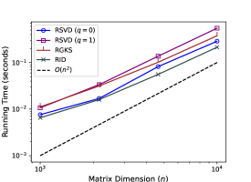
Figure 2: Runtime comparison between low-rank approximation algorithms applied to four square matrices with dimensions ranging from 1,000 to 10,000. Each data point is the average runtime over 10 low-rank approximations of the same matrix. All tests used the same approximation rank $k=50$, and all RSVD’s (including the ones internal to RGKS) were computed with oversampling $p=5$. RID was also computed with oversampling $p=5$, in the sense of using a Gaussian sketching matrix of dimension $(k+p)\times m$. Tests were run using Julia on a 2.9 GHz Intel i7-10700 CPU, with 16 GB of available RAM. All algorithms were precompiled with a dry-run before making runtime measurements.

Leverage score sampling (LSS) is very similar to RGKS in its design, since both algorithms select columns using a randomized procedure involving the right singular vectors of ${\mathbf{A}}$. We argue that the RGKS column selection strategy is more effective at optimizing the term $\sigma_{\mathrm{min}}({\mathbf{V}}_{J,\,1:k})$ which appears in bounds such as those in Eq. 1, as well as implicitly in Theorem 6.1 and Theorem 6.5. This is because RGKS approximates an RRQR factorization of ${\mathbf{V}}_{k}^{\mathrm{T}}$, which accounts for correlations between the rows of ${\mathbf{V}}_{k}$. As such, $\sigma_{\mathrm{min}}({\mathbf{V}}_{J,\,1:k})$ is maximized more effectively. In contrast, LSS only considers the row norms of ${\mathbf{V}}_{k}$. Therefore, while its sampling strategy may be effective at maximizing $\|{\mathbf{V}}_{J,\,1:k}\|_{\mathrm{F}}$, the row subset may nevertheless be near singular. For example, if ${\mathbf{V}}_{k}$ possesses two large-norm rows which are nearly colinear, then LSS is likely to pick a skeleton index subset encompassing both of these rows, significantly decreasing the value of $\sigma_{\mathrm{min}}({\mathbf{V}}_{J,\,1:k})$. In GKS and RGKS, this is prevented by the orthogonalization procedure inherent in the RRQR factorization.

5 Numerical Comparison of Algorithms

We now present experiments that compare the approximation error of RSVD, RGKS, and LSS across variations in the approximation rank and structural properties of the input matrix. For these experiments, an $n\times n$ test matrix ${\mathbf{A}}$ was generated by setting ${\mathbf{A}}={\mathbf{U}}{\mathbf{\Sigma}}{\mathbf{V}}^{\mathrm{T}}$, where ${\mathbf{U}}$ was an orthogonalization of a Gaussian random matrix. The matrix ${\mathbf{\Sigma}}$ was constructed using several different singular value decay profiles, and ${\mathbf{V}}$ was constructed with varying coherence levels. For perfectly coherent ${\mathbf{V}}$ we used permutation matrices, and for perfectly incoherent ${\mathbf{V}}$ we used normalized Hadamard matrices, i.e., orthogonal matrices whose entries are all $\pm 1/\sqrt{n}$. To explore intermediate values of coherence, ${\mathbf{V}}$ was set to be an orthogonalized convex combination of a permutation matrix and a normalized Hadamard matrix. Orthogonalization was done using a polar decomposition, so as to approximately preserve coherence structure in ${\mathbf{V}}$.

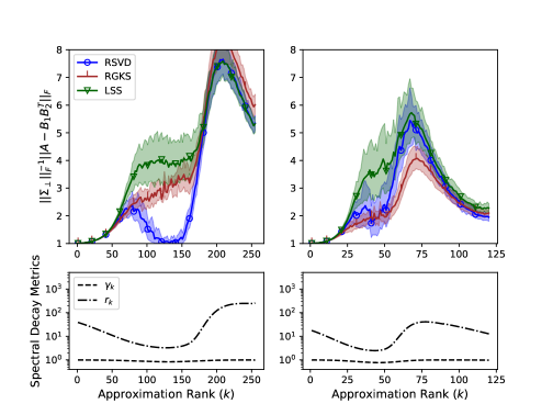
Figure 12: Spectral norm error suboptimality for $256\times 256$ test matrices with identical coherence levels. Each point is the mean accuracy over 100 approximations of the same matrix, with shaded regions indicating 10% and 90% quantiles of the error distribution. All instances of LSS and RSVD, including those internal to RGKS, were computed with oversampling $p=\lceil k/10\rceil$ and no power iteration.

Figure 3 shows how the performance of RSVD, RGKS, and LSS (relative to optimality) varies as a function of the approximation rank $k$ for two test matrices having different singular spectra. The performance comparison between RSVD and RGKS is strongly affected by singular spectrum decay; for example, for the rapidly decaying singular spectrum in the left column, RGKS greatly outperforms RSVD in regions with large singular value gaps. This behavior is reversed in the right column, which corresponds to a slower singular value decay. Notice that the RGKS error is, to a very rough approximation, inversely proportional to $r_{k}$; Theorem 6.5 will formalize this observation in an error bound. An interesting point of comparison is Fig. 12 in the appendix, which shows that the dependence on $r_{k}$ is different when errors are measured in the spectral norm.

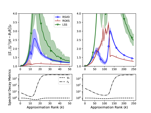
Figure 3: Frobenius norm error suboptimality, $\|{\mathbf{\Sigma}}_{\perp}\|_{\mathrm{F}}^{-1}\|{\mathbf{A}}-{\mathbf{B}}_{1}{\mathbf{B}}_{2}^{\mathrm{T}}\|_{\mathrm{F}}$, for two different $4096\times 4096$ test matrices with identical coherence levels. For comparison with Fig. 4, the coherence at $k=20$ was $c_{20}\approx 0.16$. Each point is the mean accuracy over 100 approximations of the same matrix is plotted, with shaded regions indicating 10% and 90% quantiles of the error distribution. All instances of LSS and RSVD, including those internal to RGKS, were computed with oversampling $p=\lceil k/10\rceil$. See Fig. 12 in the appendix for spectral norm errors.

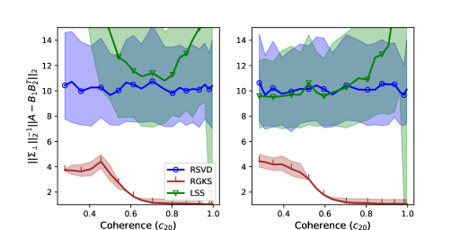
Figure 11: Spectral norm error suboptimality for square matrices of dimension 256 (left) and 252 (right). All of the matrices’ singular spectra were identical in the first 252 entries. Each data point is the average error over 100 approximations of the same matrix, with shaded regions giving 10% and 90% quantiles of the error distribution. All algorithms used oversampling $p=2$ and no power iterations.

To complement Fig. 3, Fig. 4 illustrates the effects of subspace geometry. This figure prominently shows that RSVD is completely insensitive to changes in coherence–as expected. In contrast, RGKS and LSS are much more sensitive to it. RGKS achieves its smallest approximation errors when the right singular subspace is highly coherent, and has higher approximation errors when the subspace is incoherent. However, it is important to note that the behavior at extremely low coherence levels is dependent on the finer details of the subspace construction. This is obvious for LSS in Fig. 4; in the left-hand plot, where incoherent subspaces were constructed using convex combinations with a $4096\times 4096$ Hadamard matrix, low coherence results in extremely high LSS errors. The opposite is true in the right-hand plot, where the construction used $4032\times 4032$ Hadamard matrices. Figure 4 does not show obvious differences across subspace constructions for RGKS, but we encourage the reader to examine Figs. 5 and 6, or Fig. 11 in the appendix, where the use of smaller Hadamard matrices makes these differences more apparent. We interpret these differences in behavior as a consequence of the unique sign patterns inherent to Hadamard matrices, with different Hadamard constructions having sign patterns that affect the value of $\sigma_{\mathrm{min}}({\mathbf{V}}_{J,\,1:k})$. Note that the $4096\times 4096$ test matrices in the left-hand plot of Fig. 4 had identical singular spectra to the $4096\times 4096$ test matrix used in the left-hand plot if Fig. 3. In this sense, the left-hand plots of Figs. 3 and 4 are cross-sections of each other at $k=20$ and $c_{20}\approx 0.16$.

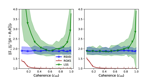
Figure 4: Frobenius norm error suboptimality, $\|{\mathbf{\Sigma}}_{\perp}\|_{\mathrm{F}}^{-1}\|{\mathbf{A}}-{\mathbf{B}}_{1}{\mathbf{B}}_{2}^{\mathrm{T}}\|_{\mathrm{F}}$, for approximations computed by RSVD, RGKS, and LSS at $k=20$, with varying coherence levels in the input matrix. The left-hand plot used square test matrices of dimension $n=4096$, and the right-hand plot used square matrices with $n=4032$. All test matrices had identical singular spectra in the first 4032 entries. Each data point is the average error over 100 approximations of the same matrix, with shaded regions giving 10% and 90% quantiles of the error distribution. All algorithms used oversampling $p=2$. See Fig. 11 in the appendix for spectral norm errors.

6 Structure-Aware Analyses of Interpolative Decompositions

Here we develop and analyze error bounds which capture the effects of singular subspace geometry (Section 6.1), residual stable rank (Section 6.2), and singular value decay (Section 6.3).

6.1 The Effects of Subspace Geometry

To develop an interpolative decomposition error bound which captures the effects of subspace geometry, the main idea is to view interpolative decomposition as a process of approximating one subspace by another, namely, approximating $\operatorname{range}({\mathbf{A}})$ by the span of a small number of ${\mathbf{A}}$’s columns. By connecting this to a different problem which involves approximating the leading right singular subspace, we will see that the geometry of this subspace plays an important role in determining the accuracy of the original interpolative decomposition. To work in this setting, we assume that $\sigma_{k}({\mathbf{A}})>\sigma_{k+1}({\mathbf{A}})$ so that the leading right singular subspace ${\mathcal{V}}_{k}$ is well defined. Given this assumption, we define a subspace ${\mathcal{I}}_{J}\subseteq{\mathbb{R}}^{n}$ encoding the choice of skeleton columns as

(9) $${\mathcal{I}}_{J}=\operatorname{span}\{{\mathbf{e}}_{j}\,:\,j\in J\}.$$

We now state the main result of this section below as Theorem 6.1.

Theorem 6.1.

Choose $k\leq n/2$ such that $\sigma_{k}({\mathbf{A}})>\sigma_{k+1}({\mathbf{A}})$, and let $\varphi_{\mathrm{max}}$ be the largest principal angle between ${\mathcal{I}}_{J}$ and ${\mathcal{V}}_{k}$. If $\varphi_{\mathrm{max}}<\pi/2$, then

$$\|{\mathbf{A}}-{\mathbf{A}}_{:,\,J}({\mathbf{A}}_{:\,J})^{\dagger}{\mathbf{A}}\|_{2}\leq\|{\mathbf{\Sigma}}_{\perp}\|_{2}\sec\varphi_{\mathrm{max}}.$$

Proof 6.2.

As explained below, this is an equivalent statement of [21, Theorem 1.5]. For a self-contained proof, refer to Section A.6.

Theorem 6.1 shows that the problem of choosing columns of ${\mathbf{A}}$ whose span approximates $\operatorname{range}({\mathbf{A}})$ is related to the problem of choosing elementary unit vectors whose span approximates the right singular subspace ${\mathcal{V}}_{k}$. Leverage scores provide some amount of information on this problem, in that $\ell_{j}$ measures the degree to which ${\mathbf{e}}_{j}$ is aligned with ${\mathcal{V}}_{k},$ as seen from the relation

$$\ell_{j}=\|{\mathbf{V}}_{j,\,1:k}\|_{2}=\|{\mathbf{V}}_{j,\,1:k}({\mathbf{V}}_{:,\,1:k})^{\mathrm{T}}\|_{2}=\|{\mathbf{e}}_{j}^{\mathrm{T}}{\mathbf{V}}_{k}{\mathbf{V}}_{k}^{\mathrm{T}}\|_{2}.$$

Lemma 6.3 allows us to formalize the connections between leverage scores and $\varphi_{\mathrm{max}}$.

Lemma 6.3.

Choose $k\leq n/2$ with $\sigma_{k}({\mathbf{A}})>\sigma_{k+1}({\mathbf{A}})$. If $\varphi_{1}\leq\ldots\leq\varphi_{k}$ are the principal angles between ${\mathcal{I}}_{J}$ and ${\mathcal{V}}_{k}$, then

$$\cos\varphi_{i}=\sigma_{i}({\mathbf{V}}_{J,\,1:k})$$

for $1\leq i\leq k$. Furthermore, ${\mathbf{V}}_{J,\,1:k}$ is invertible if and only if $\max_{i}\varphi_{i}<\pi/2$, in which case

$$\tan\varphi_{k-i+1}=\sigma_{i}({\mathbf{V}}_{[n]\setminus J,\,1:k}({\mathbf{V}}_{J,\,1:k})^{-1})$$

for $1\leq i\leq k$.

Proof 6.4.

Refer to Section A.4.

An important consequence of Lemma 6.3 is that $\cos\varphi_{\mathrm{max}}=\sigma_{\mathrm{min}}({\mathbf{V}}_{J,\,1:k})$. This, together with Eq. 7, proves the equivalence of Theorem 6.1 and [21, Theorem 1.5].

Lemma 6.3 provides a means of quantifying the effects of subspace geometry on interpolative decomposition accuracy, because it implies upper and lower bounds on $\sec\varphi_{\mathrm{max}}$ that depend on leverage scores and coherence. Recall that coherence at rank $k$ is defined as $c_{k}=\max_{1\leq j\leq n}\ell_{j}$. In the case of low coherence, we can place a lower bound on $\sec\varphi_{\mathrm{max}}$ by using Lemma 6.3, together with the fact that the minimum singular value of a matrix cannot exceed the minimum row norm:

$$\sec\varphi_{\mathrm{max}}=\frac{1}{\sigma_{\mathrm{min}}({\mathbf{V}}_{J,\,1:k})}\geq\frac{1}{\min_{j\in J}\ell_{j}}\geq c_{k}^{-1}.$$

In the case of near-minimal coherence, we have $c_{k}\leq(1+\varepsilon)\sqrt{n^{-1}k}$ for some small number $\varepsilon>0$. Then $\sec\varphi_{\mathrm{max}}\geq(1+\varepsilon)^{-1}\sqrt{k^{-1}n}$, and as expected for the incoherent case, this bound holds independent of the choice of $J$.

For the case where there are $k$ leverage scores with values near unity and corresponding to column indices $J=\{j_{1},\,\ldots,\,j_{k}\}$, we can bound $\sec\varphi_{\mathrm{max}}$ from above. Using Lemma 6.3,

$$\sum_{i=1}^{k}\cos^{2}\varphi_{i}=\sum_{i=1}^{k}\sigma_{i}({\mathbf{V}}_{J,\,1:k})^{2}=\|{\mathbf{V}}_{J,\,1:k}\|_{\mathrm{F}}^{2}=\sum_{j\in J}\ell_{j}^{2}.$$

This implies that $\cos^{2}\varphi_{\mathrm{max}}={\textstyle\sum_{j\in J}\ell_{j}^{2}-\sum_{i\neq i_{\mathrm{max}}}\cos^{2}\varphi_{i}}$, where $i_{\mathrm{max}}\in\operatorname*{arg\,max}_{i}\varphi_{i}$. Inserting $\cos\varphi_{i}\leq 1$ for $i\neq i_{\mathrm{max}}$, and assuming the skeleton columns have large enough leverage scores that $\sum_{j\in J}\ell_{j}^{2}\geq k-1$, we obtain

(10) $$\sec\varphi_{\mathrm{max}}\leq\frac{1}{\sqrt{1-\sum_{j\in J}(1-\ell_{j}^{2})}},$$

a bound which is small when $\ell_{j}\approx 1$ for all $j\in J$. Choosing $k$ indices with leverage scores near unity is sufficient, but emphatically not necessary, for $\sec\varphi_{\mathrm{max}}$ to be small. For example, Fig. 4 shows that even at the minimum of coherence, when there are no leverage scores near unity, RGKS can still attain close to optimal error.

Although bounds on $\sec\varphi_{\mathrm{max}}$ are useful in describing the effects of coherence and leverage scores, $\sec\varphi_{\mathrm{max}}$ itself can be overly pessimistic as a bound on approximation error (relative to $\|{\mathbf{\Sigma}}_{\perp}\|_{2}$). To see this, consider any subset $I\subseteq J$ of size $k-t$, and assuming that $\sigma_{k-t}({\mathbf{A}})>\sigma_{k-t+1}({\mathbf{A}})$, let $\varphi_{\mathrm{max}}^{(I)}$ denote the largest principal angle between ${\mathcal{V}}_{k-t}$ and ${\mathcal{I}}_{I}$. Using Theorem 6.1, together with the fact that interpolative decomposition error is monotone decreasing as skeleton columns are added,

$$\|{\mathbf{A}}-{\mathbf{A}}_{:,\,J}({\mathbf{A}}_{:,\,J})^{\dagger}{\mathbf{A}}\|_{2} \leq\|{\mathbf{A}}-{\mathbf{A}}_{:,\,I}({\mathbf{A}}_{:,\,I})^{\dagger}{\mathbf{A}}\|_{2}$$

$$\leq\sigma_{k-t+1}({\mathbf{A}})\sec\varphi_{\mathrm{max}}^{(I)}$$

(11) $$=\frac{\|{\mathbf{\Sigma}}_{\perp}\|_{2}\sec\varphi_{\mathrm{max}}^{(I)}}{\gamma_{k-t+1,\,k+1}},$$

where $\gamma_{i,\,j}=\sigma_{j}({\mathbf{A}})/\sigma_{i}({\mathbf{A}})$. Equivalently, because of Lemma 6.3,

(12) $$\|{\mathbf{A}}-{\mathbf{A}}_{:,\,J}({\mathbf{A}}_{:,\,J})^{\dagger}{\mathbf{A}}\|_{2}\leq\frac{\|{\mathbf{\Sigma}}_{\perp}\|_{2}}{\gamma_{k-t+1,\,k+1}\sigma_{\mathrm{min}}({\mathbf{V}}_{I,\,1:k-t})}.$$

Equation Eq. 11 shows that when $\sigma_{k-t+1}({\mathbf{A}})\approx\sigma_{k+1}({\mathbf{A}})$, obtaining a near-optimal approximation does not necessarily require that $\varphi_{\mathrm{max}}$ is small. Rather, it is sufficient that a smaller singular subspace ${\mathcal{V}}_{k-t}$ is well-approximated by some smaller subset of elementary unit vectors, corresponding to a small value of $\varphi_{\mathrm{max}}^{(I)}$. From the perspective of minimal singular values, equation Eq. 12 shows that a large value of $\sigma_{\mathrm{min}}({\mathbf{V}}_{J,\,1:k})$ is not strictly necessary for obtaining near-optimal approximation error. Instead, it is sufficient that ${\mathbf{V}}_{J,\,1:k}$ contains a submatrix ${\mathbf{V}}_{I,\,1:k-t}$ whose minimal singular value is large, for some $t$ such that $\sigma_{k-t+1}({\mathbf{A}})\approx\sigma_{k+1}({\mathbf{A}})$. This is easiest to achieve when $t$ is chosen as large as possible while maintaining $\sigma_{k-t+1}({\mathbf{A}})\approx\sigma_{k+1}({\mathbf{A}})$.

We end this subsection with Fig. 5, which compares the error bound in Theorem 6.1 to the actual error for approximations computed with RGKS. In the right-hand plot, we see that the error bound accurately reflects the changes in approximation accuracy as subspace geometry (measured by coherence) is varied. However, note how the looseness of $\sec\varphi_{\mathrm{max}}$ as a bound on approximation error (relative to $\|{\mathbf{\Sigma}}_{\perp}\|_{2}$) is illustrated in the left-hand plot, particularly for small approximation ranks.

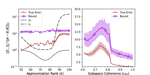
Figure 5: Spectral norm error suboptimality of RGKS, $\|{\mathbf{\Sigma}}_{\perp}\|_{2}^{-1}\|{\mathbf{A}}-{\mathbf{B}}_{1}{\mathbf{B}}_{2}^{\mathrm{T}}\|_{2}$, versus the bound in Theorem 6.1. Each data point is the mean error over 100 approximations of the same $256\times 256$ matrix, or the mean error bound as evaluated over each of the 100 approximations. Shaded regions indicate 10% and 90% quantiles. All tests in the left-hand graph used the same test matrix, and all test matrices across both graphs had identical singular spectra. All RSVD’s (including those internal to RGKS) were computed using oversampling $p=\lceil k/10\rceil$ and no power iterations.

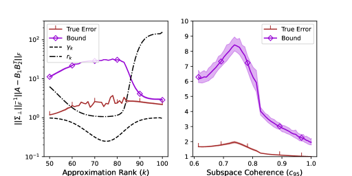
Figure 6: Frobenius norm error suboptimality of RGKS, $\|{\mathbf{\Sigma}}_{\perp}\|_{\mathrm{F}}^{-1}\|{\mathbf{A}}-{\mathbf{B}}_{1}{\mathbf{B}}_{2}^{\mathrm{T}}\|_{\mathrm{F}}$, versus the bound in Theorem 6.5. Each data point is the mean error over 100 approximations of the same $256\times 256$ matrix, or the mean error bound as evaluated over each of the 100 approximations. Shaded regions indicate 10% and 90% quantiles. All tests in the left-hand graph used the same test matrix, and all test matrices across both graphs had identical singular spectra. All RSVD’s (including those internal to RGKS) were computed using oversampling $p=\lceil k/10\rceil$ and no power iterations.

6.2 Subspace Geometry and Stable Rank

The bound in the previous section captures the effects of subspace structure, but fails to capture the effects of spectral decay structures such as singular value gap and stable rank. Figure 5, for example, shows that the relative spectral error of RGKS tends to be greatest in or near regions with both high stable rank and a significant singular value gap, while the plot of the corresponding error bound shows no such dependence on the singular spectrum. We now present a bound which captures the combined effects of subspace geometry and singular spectral decay, where spectral decay is measured by the residual stable rank; this is accomplished by shifting our analysis to errors measured in the Frobenius norm. We state the result below in Theorem 6.5.

Theorem 6.5.

Choose $k\leq n/2$ such that $\sigma_{k}({\mathbf{A}})>\sigma_{k+1}({\mathbf{A}})$, and let $\varphi_{1},\,\ldots,\,\varphi_{k}$ be the principal angles between ${\mathcal{I}}_{J}$ and ${\mathcal{V}}_{k}$. If $\max_{i}\varphi_{i}<\pi/2$, then

(13) $$\|{\mathbf{A}}-{\mathbf{A}}_{:,\,J}({\mathbf{A}}_{:,\,J})^{\dagger}{\mathbf{A}}\|_{\mathrm{F}}\leq\|{\mathbf{\Sigma}}_{\perp}\|_{\mathrm{F}}\sqrt{1+\frac{1}{r_{k}}\sum_{i=1}^{k}\tan^{2}\varphi_{i}},$$

where $r_{k}=\|{\mathbf{\Sigma}}_{\perp}\|_{\mathrm{F}}^{2}/\|{\mathbf{\Sigma}}_{\perp}\|_{2}^{2}$ is the residual stable rank.

Proof 6.6.

Refer to Section A.7.

Theorem 6.5 depends on subspace geometry effects through $\tan\varphi_{1},\,\ldots,\,\tan\varphi_{k}$, and depends on all of the principal angles between ${\mathcal{I}}_{J}$ and ${\mathcal{V}}_{k}$. (Whereas the bound from Section 6.1 depended on only the largest angle.) Unlike the previous bound, Theorem 6.5 also incorporates the effects of stable rank in the form of a factor $r_{k}^{-1}$ that attenuates the impact of subspace geometry. This suggests that when errors are measured in the Frobenius norm, a near-optimal interpolative decomposition is easier to obtain at approximation ranks corresponding to a high value of $r_{k}$, an idea which is confirmed by the experiments plotted in Fig. 3. Further confirmation is offered by Fig. 6, which plots the actual RSVD error compared with the error bound in Theorem 6.5 as the approximation rank and coherence are varied.

6.3 An Error Bound for Flat Singular Spectra

In this section we bound the approximation error of interpolative decompositions at ranks where the absence of singular value decay renders Theorem 6.1 and Theorem 6.5 inapplicable. In addition, the bound in this section reveals that the relative error of a low-rank approximation is strongly related to the spectral properties of the residual error matrix. While it is common for error bounds to depend on the spectrum of the optimal residual singular value matrix ${\mathbf{\Sigma}}_{\perp}$, the bound in this section depends on the spectrum of the actual residual matrix.

Consider a subspace ${\mathcal{W}}\subseteq{\mathbb{R}}^{m}$ with $\dim{\mathcal{W}}=k<m$, and define ${\mathbf{E}}={\mathbf{A}}-{\mathbf{P}}_{\mathcal{W}}{\mathbf{A}}$, where ${\mathbf{P}}_{\mathcal{W}}$ is the orthogonal projection matrix onto ${\mathcal{W}}$. We can interpret ${\mathbf{E}}$ as the residual of a low-rank approximation computed by projecting the columns of ${\mathbf{A}}$ into ${\mathcal{W}}$. Furthermore, we define the truncated condition number at level $i$ of a matrix ${\mathbf{M}}$ as $\kappa({\mathbf{M}},\,i)\mathrel{\hbox to0.0pt{\raisebox{1.29167pt}{$\cdot$}\hss}\raisebox{-1.29167pt}{$\cdot$}}=\sigma_{1}({\mathbf{M}})/\sigma_{i}({\mathbf{M}})$. We can now state Theorem 6.7 below, the main result of this section.

Theorem 6.7.

If $\sigma_{k+1}({\mathbf{E}})>0$, then $\|{\mathbf{E}}\|_{2}\leq\|{\mathbf{\Sigma}}_{\perp}\|_{2}\kappa({\mathbf{E}},\,k+1)$.

Proof 6.8.

Refer to Section A.1.

Figure 7 illustrates the approximation error of RGKS versus the bound in Theorem 6.7. At approximation ranks where there is a large singular value gap, the bound is extremely loose. But in certain regions where the singular spectrum does not decay (or decays slowly), the bound is strikingly tight. This stands in sharp contrast to Theorem 6.1 and Theorem 6.5, which required a singular value gap for the error bounds to even be well-defined. Lemma 6.9 helps explain why Theorem 6.7 provides such a sharp bound on the approximation error when the singular specturm is flat.

Lemma 6.9.

If $1\leq i\leq\min\{m,\,n\}-k$, then $\sigma_{i}({\mathbf{E}})\geq\sigma_{k+i}({\mathbf{A}})$.

Proof 6.10.

Refer to Section A.2.

Suppose, now, that the singular spectrum of ${\mathbf{A}}$ has very slow decay (or no decay), so that $\sigma_{k+1}({\mathbf{A}})\leq(1+\varepsilon)\sigma_{2k+1}({\mathbf{A}})$ for some small number $\varepsilon>0$. Assuming that $2k+1\leq\min\{m,\,n\}$, Lemma 6.9 shows that $\sigma_{k+1}({\mathbf{E}})\geq\sigma_{2k+1}({\mathbf{A}})$. We then have

$$\|{\mathbf{E}}\|_{2}=\|{\mathbf{\Sigma}}_{\perp}\|_{2}\frac{\sigma_{1}({\mathbf{E}})}{\sigma_{k+1}({\mathbf{A}})}\geq\|{\mathbf{\Sigma}}_{\perp}\|_{2}\frac{\sigma_{1}({\mathbf{E}})}{(1+\varepsilon)\sigma_{2k+1}({\mathbf{A}})}\geq\|{\mathbf{\Sigma}}_{\perp}\|_{2}\frac{\kappa({\mathbf{E}},\,k+1)}{1+\varepsilon},$$

meaning that the bound in Theorem 6.7 tight to within a factor of $1+\varepsilon$.

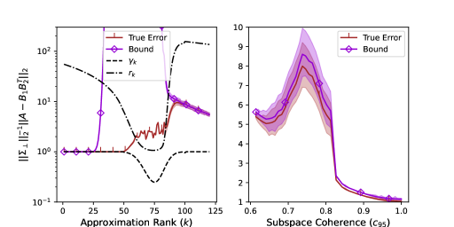
Figure 7: Spectral norm error suboptimality of RGKS, $\|{\mathbf{\Sigma}}_{\perp}\|_{2}^{-1}\|{\mathbf{A}}-{\mathbf{B}}_{1}{\mathbf{B}}_{2}^{\mathrm{T}}\|_{2}$, versus the bound in Theorem 6.7. Each data point is the mean error over 100 approximations of the same $256\times 256$ matrix, or the mean error bound as evaluated over each of the 100 approximations. Shaded regions indicate 10% and 90% quantiles. Although the bound in Theorem 6.7 has no explicit dependence on coherence, this figure illustrates that it retains its quality across coherence levels. All tests in the left-hand graph used the same test matrix, and all test matrices across both graphs had identical singular spectra. All RSVD’s (including those internal to RGKS) were computed using oversampling $p=\lceil k/10\rceil$ and no power iterations.

7 Analysis of RGKS

The error bounds discussed so far are applicable to any interpolative decomposition, regardless of the algorithm used to compute it. If, however, the decomposition is computed by RGKS, then these bounds become especially useful in in that they depend on quantities that are optimized more directly in RGKS than in other interpolative decomposition algorithms. This allows for the development of more refined error bounds for RGKS. Section 7.1 will begin by developing bounds for GKS, where the lack of randomization makes things more straightforward. Section 7.2 then extends the GKS error bounds to RGKS by building off of a preexisting error analysis for RSVD. In practice, we find that RGKS is more robust to randomization errors than the arguments in Section 7.2 would suggest, and Section 7.3 develops theory which offers partial explanations for this behavior. Section 7.4 presents numerical experiments which lend support to the arguments in Section 7.3.

7.1 Analysis of GKS

Theorem 6.1 bounds the spectral norm error of a general interpolative decomposition in terms of $\sec\varphi_{\mathrm{max}}$, where $\varphi_{\mathrm{max}}$ is the largest principal angle between ${\mathcal{V}}_{k}$ and ${\mathcal{I}}_{J}\mathrel{\hbox to0.0pt{\raisebox{1.29167pt}{$\cdot$}\hss}\raisebox{-1.29167pt}{$\cdot$}}=\operatorname{span}\{{\mathbf{e}}_{j}\,:\,j\in J\}$. Unlike in other interpolative decomposition algorithms, the column selection strategy of GKS can be viewed directly in terms of minimizing $\varphi_{\mathrm{max}}$. Indeed, if we write the RRQR factorization in line 2 of GKS (Algorithm 1) as

$${\mathbf{V}}_{k}^{\mathrm{T}}\mathbf{{\Pi}}=\begin{bmatrix}({\mathbf{V}}_{J,\,1:k})^{\mathrm{T}}&({\mathbf{V}}_{[n]\setminus J,\,1:k})^{\mathrm{T}}\end{bmatrix}={\mathbf{Q}}\begin{bmatrix}{\mathbf{R}}_{1}&{\mathbf{R}}_{2}\end{bmatrix},$$

with ${\mathbf{R}}_{1}\in{\mathbb{R}}^{k\times k}$, then Lemma 6.3 implies that $\sec\varphi_{\mathrm{max}}=(\cos\sigma_{\mathrm{min}}({\mathbf{V}}_{J,\,1:k}))^{-1}=\sigma_{\mathrm{min}}({\mathbf{R}}_{1})^{-1}$. Rank-revealing QR factorizations are designed explicitly to choose a well conditioned set of basis columns, i.e., a $J$ for which $\sigma_{\mathrm{min}}({\mathbf{R}}_{1})$ is large. In this sense, line 2 of GKS serves directly to minimize $\varphi_{\mathrm{max}}$. Quantitatively, the algorithmic guarantees of RRQR factorizations are such that $\sigma_{\mathrm{min}}({\mathbf{R}}_{1})\geq\sigma_{k}({\mathbf{V}}_{k}^{\mathrm{T}})q(n,\,k)^{-1}=q(n,\,k)^{-1}$, where $q$ is a function whose growth in $n$ is bounded by a low-degree polynomial. Therefore, Lemma 6.3 shows that $\varphi_{\mathrm{max}}\leq\arccos(q(n,\,k)^{-1})$, meaning by Theorem 6.1 that

(14) $$\|{\mathbf{A}}-{\mathbf{A}}_{:,\,J}({\mathbf{A}}_{:,\,J})^{\dagger}{\mathbf{A}}\|_{2} \leq\|{\mathbf{\Sigma}}_{\perp}\|_{2}\sec(\arccos(q(n,\,k)^{-1}))$$

$$\leq q(n,\,k)\|{\mathbf{\Sigma}}_{\perp}\|_{2}.$$

Interestingly, the same error bound holds for interpolative decompositions obtained by applying a RRQR factorization directly to the columns of ${\mathbf{A}}$, rather than to the rows of ${\mathbf{V}}_{k}$ as in GKS. This follows from equations Eq. 7 and Eq. 8. The GKS bound can be refined by considering specific RRQR factorization algorithms for which an explicit form of $q(n,\,k)$ is available. For example, if the Gu-Eisenstat algorithm [18] is used in line 2 of GKS, then the bound becomes

(15) $$\|{\mathbf{A}}-{\mathbf{A}}_{:,\,J}({\mathbf{A}}_{:,\,J})^{\dagger}{\mathbf{A}}\|_{2}\leq\|{\mathbf{\Sigma}}_{\perp}\|_{2}\sqrt{1+f^{2}k(n-k)},$$

where $f>1$ is a user-selected parameter controlling a trade-off between maximizing $\sigma_{\mathrm{min}}({\mathbf{R}}_{1})$ and minimizing runtime.

For the Frobenius norm error bound, Theorem 6.5, similar reasoning applies. In addition to terms that depend only on the singular values of ${\mathbf{A}}$, this bound depends on skeleton column choices through the term $\sum_{i}\tan^{2}\varphi_{i}$. Lemma 6.3 allows us to express this in terms of a quantity that GKS approximately optimizes:

$$\sum_{i=1}^{k}\tan^{2}\varphi_{i} =\sum_{i=1}^{k}\sigma_{i}({\mathbf{V}}_{[n]\setminus J,\,1:k}({\mathbf{V}}_{J,\,1:k})^{-1})^{2}=\sum_{i=1}^{k}\sigma_{i}({\mathbf{R}}_{2}^{\mathrm{T}}{\mathbf{R}}_{1}^{-\mathrm{T}})^{2}$$

$$=\|{\mathbf{R}}_{1}^{-1}{\mathbf{R}}_{2}\|_{\mathrm{F}}^{2}.$$

The quantity $\|{\mathbf{R}}_{1}^{-1}{\mathbf{R}}_{2}\|_{\mathrm{F}}^{2}$ measures the size of the coefficients used by the RRQR factorization to interpolate the rows of ${\mathbf{V}}_{k}$ in terms of ${\mathbf{V}}_{J,\,1:k}$. The RRQR factorization in GKS strives to minimize these coefficient magnitudes by choosing a well-conditioned row basis, and in some cases, upper-bounds are available. For example, the Gu-Eisenstat algorithm chooses $J$ such that the entries of ${\mathbf{R}}_{1}^{-1}{\mathbf{R}}_{2}$ are bounded in magnitude by $f$ [18]. This leads to the bound $\|{\mathbf{R}}_{1}^{-1}{\mathbf{R}}_{2}\|_{\mathrm{F}}\leq f\sqrt{k(n-k)}$ and, by an application of Theorem 6.5,

(16) $$\|{\mathbf{A}}-{\mathbf{A}}_{:,\,J}({\mathbf{A}}_{:,\,J})^{\dagger}{\mathbf{A}}\|_{\mathrm{F}}\leq\|{\mathbf{\Sigma}}_{\perp}\|_{\mathrm{F}}\sqrt{1+r_{k}^{-1}f^{2}k(n-k)}.$$

Notice the improvement over Eq. 15 by a factor of $r_{k}^{-1}$ inside the square-root. This improvement suggests, in a limited sense, that GKS with the Gu-Eisenstat algorithm is a near-optimal interpolative decomposition for certain classes of matrices. Specifically, it is known [10, Theorem 3] that for any $k\geq 1$ and $\varepsilon>0$, there exists a $k\times(k+1)$ matrix ${\mathbf{A}}$ such that

(17) $$\min_{K\subseteq[n],\,|K|=k}\|{\mathbf{A}}-{\mathbf{A}}_{:,\,K}({\mathbf{A}}_{:,\,K})^{\dagger}{\mathbf{A}}\|_{2}\geq\|{\mathbf{\Sigma}}_{\perp}\|_{\mathrm{F}}(1-\varepsilon)\sqrt{1+k}.$$

Therefore, the smallest interpolative decomposition error bound which can hold over all matrices and all $k$ is $\|{\mathbf{\Sigma}}_{\perp}\|_{\mathrm{F}}\sqrt{1+k}$. GKS with the Gu-Eisenstat algorithm nearly attaining this bound for matrices with large residual stable rank ($r_{k}\to n-k$).

7.2 Extension to RGKS

We now extend the analysis to RGKS, where the main challenge is to account for errors introduced by randomizing the SVD. The analysis in this section builds on well-developed theory for RSVD and uses a measure of randomization error that has been extensively studied in previous literature. However, the resulting bounds on RGKS error will only be tight when $k$ corresponds to a large singular value gap. Section 7.3 will offer two alternative analyses that can better handle shallow singular value gaps, but the first analysis uses a comparison with optimal error at a rank smaller than $k$, while the second analysis uses a measure of randomization error that is less well studied.

The column selection strategy of RGKS (Algorithm 2) is equivalent to running GKS on the rank-$k$ approximation $\widehat{{\mathbf{A}}}=\widehat{{\mathbf{U}}}_{k}\widehat{{\mathbf{\Sigma}}}_{k}\widehat{{\mathbf{V}}}_{k}^{\mathrm{T}}$ computed by RSVD in line 1. Therefore, while GKS approximately minimizes the largest angle between ${\mathcal{I}}_{J}$ and ${\mathcal{V}}_{k}$, RGKS instead minimizes the largest angle between ${\mathcal{I}}_{J}$ and $\widehat{{\mathcal{V}}}_{k}$, where $\widehat{{\mathcal{V}}}_{k}=\operatorname{range}(\widehat{{\mathbf{V}}}_{k})$ is the RSVD estimate of ${\mathcal{V}}_{k}$. If we denote this largest angle by $\widehat{\varphi}_{\mathrm{max}}$, then extending the analysis of the previous section means bounding $\varphi_{\mathrm{max}}$ from above in terms of $\widehat{\varphi}_{\mathrm{max}}$. A bound of this sort must depend on the accuracy of the singular vector estimates produced by RSVD; this can be accounted for using $\theta_{\mathrm{max}}$, the largest principal angle between ${\mathcal{V}}_{k}$ and $\widehat{{\mathcal{V}}}_{k}$. Principal angles have long been used as a measure of subspace approximation errors, most famously in the perturbation theory developed by Davis and Kahan [8], Stewart [29], and Wedin [32]. Recent years have also seen the developments of principal angle bounds that take into account the algorithmic details of RSVD [12, 27].

Using $\theta_{\mathrm{max}}$ to quantify randomization error, Theorem 7.1 provides a perturbation bound for extending the GKS analysis to RGKS.

Theorem 7.1.

If $k\leq n/2$ is such that $\sigma_{k}({\mathbf{A}})>\sigma_{k+1}({\mathbf{A}})$, then

$$\varphi_{\mathrm{max}}\leq\widehat{\varphi}_{\mathrm{max}}+\theta_{\mathrm{max}}.$$

Proof 7.2.

An elementary proof is given in Section A.8. This result also follows from the more general triangle inequalities proven in [25] for symmetric gauge functions over principal angles.

Combining Theorem 6.1 with Theorem 7.1, we obtain the RGKS error bound

(18) $$\|{\mathbf{A}}-{\mathbf{A}}_{:,\,J}({\mathbf{A}}_{:,\,J})^{\dagger}{\mathbf{A}}\|_{2}\leq\|{\mathbf{\Sigma}}_{\perp}\|_{2}\sec(\widehat{\varphi}_{\mathrm{max}}+\theta_{\mathrm{max}}).$$

Line 2 of RGKS ensures that $\widehat{\varphi}_{\mathrm{max}}\leq\arccos(q(n,\,k)^{-1})$, where the form of $q$ depends on the specific algorithm used to compute the RRQR factorization. In practice, this bound on $\widehat{\varphi}_{\mathrm{max}}$ may be quite loose. For a Frobenius norm bound, we replace the upper bound in Theorem 6.5 with the larger bound $\|{\mathbf{\Sigma}}_{\perp}\|_{2}(1+kr_{k}^{-1}\tan^{2}\varphi_{\mathrm{max}})^{1/2}$. Then, applying Theorem 7.1, we have

(19) $$\|{\mathbf{A}}-{\mathbf{A}}_{:,\,J}({\mathbf{A}}_{:,\,J})^{\dagger}{\mathbf{A}}\|_{\mathrm{F}}\leq\|{\mathbf{\Sigma}}_{\perp}\|_{\mathrm{F}}\sqrt{1+\frac{k}{r_{k}}\tan^{2}(\widehat{\varphi}_{\mathrm{max}}+\theta_{\mathrm{max}})}.$$

The usefulness of these bounds depends on the size of $\theta_{\mathrm{max}}$. In particular, for these bounds to be non-vacuous, the RSVD in line 1 of RGKS must be accurate enough that $\theta_{\mathrm{max}}<\pi/2-\widehat{\varphi}_{\mathrm{max}}$. Saibaba [27] has shown that

(20) $${\mathbb{E}}[\sin\theta_{\mathrm{max}}]\leq\frac{\gamma_{k}^{2q+2}C(p)}{\sqrt{1+\gamma_{k}^{4q+4}C(p)^{2}}},$$

where $q$ is the RSVD power iteration number, $p$ is the oversampling parameter, and $C$ is a decreasing function of $p$. This result shows that $\theta_{\mathrm{max}}$ is small with high probability when $\gamma_{k}\ll 1$, but this is unfortunately not the case when $\gamma_{k}\approx 1$. The situation is illustrated in Fig. 8, which shows $\varphi_{\mathrm{max}},\,\widehat{\varphi}_{\mathrm{max}}$, and $\widehat{\varphi}_{\mathrm{max}}+\theta_{\mathrm{max}}$ as a function of $k$ for a test matrix having widely varying values of $\gamma_{k}$. At $k$ where $\gamma_{k}$ is very small, $\widehat{\varphi}_{\mathrm{max}}+\theta_{\mathrm{max}}$ bounds $\varphi_{\mathrm{max}}$ well below $\pi/2$. But as $\gamma_{k}$ approaches unity, $\widehat{\varphi}_{\mathrm{max}}+\theta_{\mathrm{max}}$ rapidly exceeds $\pi/2$.

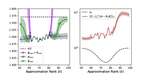
Figure 8: Principal angles and approximation errors for approximations computed by RGKS at different ranks. All tests were run on the same $256\times 256$ matrix, and the RSVD’s internal to RGKS were computed with oversampling $p=\lceil k/10\rceil$ and no power iterations. Each data point is the mean over 100 independent runs of RGKS, with shaded regions indicating 10% and 90% quantiles.

7.3 Robustness of RGKS to Noise

When $\gamma_{k}\approx 1$, the actual error of RGKS may be smaller than the previous section’s analysis would suggest. For example, consider Fig. 8, and in particular, examine the values of $k$ where $\widehat{\varphi}_{\mathrm{max}}+\theta_{\mathrm{max}}$ approaches $\pi/2$. In this limit, the error bounds in Eq. 18 and Eq. 19 diverge to $+\infty$. However, $\varphi_{\mathrm{max}}$ itself does not approach $\pi/2$ at these ranks, and more importantly, the actual RGKS error remains reasonably close to optimal.

One potential explanation for this behavior is that even when the RSVD in line 1 of RGKS estimates ${\mathcal{V}}_{k}$ poorly, a smaller singular subspace ${\mathcal{V}}_{k-t}$ might be estimated quite well. To formalize this, assume that $\sigma_{k-t}({\mathbf{A}})>\sigma_{k-t+1}({\mathbf{A}})$ so that ${\mathcal{V}}_{k-t}$ is well-defined. Let $\widehat{{\mathcal{V}}}_{k-t}$ denote the subspace spanned by the first $k-t$ right singular vectors estimated by the RSVD, and define $\theta_{\mathrm{max}}^{(k-t)}$ to be the largest principal angle between ${\mathcal{V}}_{k-t}$ and $\widehat{{\mathcal{V}}}_{k-t}$. Because the RSVD is computed at rank $k$ with oversampling $p$, this construction of $\widehat{{\mathcal{V}}}_{k-t}$ is equivalent to running RSVD at rank $k-t$ with oversampling $p+t$. Therefore, Eq. 20 shows that

(21) $${\mathbb{E}}[\sin\theta_{\mathrm{max}}^{(k-t)}]\leq\frac{\gamma_{k-t}^{2q+2}C(p+t)}{\sqrt{1+\gamma_{k-t}^{4q+4}C(p+t)^{2}}}.$$

If $\gamma_{k-t}\ll 1$, then this bound implies that $\theta_{\mathrm{max}}^{(k-t)}$ is small with high probability, regardless of the value of $\gamma_{k}$. This is in contrast to $\theta_{\mathrm{max}}$, which is essentially uncontrolled when $\gamma_{k}\approx 1$. The extra oversampling in Eq. 21 as compared to Eq. 20 makes the difference between $\theta_{\mathrm{max}}^{(k-t)}$ and $\theta_{\mathrm{max}}$ even more pronounced. A proof in Section A.9 shows that RGKS satisfies the error bound

(22) $$\|{\mathbf{A}}-{\mathbf{A}}_{:,\,J}({\mathbf{A}}_{:,\,J})^{\dagger}{\mathbf{A}}\|_{2}\leq\frac{\|{\mathbf{\Sigma}}_{\perp}\|_{2}}{\gamma_{k-t+1,\,k+1}}\sec(\widehat{\varphi}_{\mathrm{max}}+\theta_{\mathrm{max}}^{(k-t)}),$$

where $\gamma_{k-t+1,\,k+1}=\sigma_{k+1}({\mathbf{A}})/\sigma_{k-t+1}({\mathbf{A}})$. Because of the difference between $\theta_{\mathrm{max}}$ and $\theta_{\mathrm{max}}^{(k-t)}$, this bound may not suffer from the divergence to $+\infty$ when the spectrum is flat after $\sigma_{k}({\mathbf{A}})$. However, this analysis pays the price of comparing to optimal error at a rank smaller than $k$, as reflected by the presence of $\gamma_{k-t+1,\,k+1}$ in the denominator of Eq. 22.

Another potential explanation for why RGKS error can remain small, even in the absence of rapid singular value decay, is that the upper bound on $\varphi_{\mathrm{max}}$ in Theorem 7.1 may be overly pessimistic given the kinds of subspace errors that RSVD commits. This is reasonable to expect given that $\theta_{\mathrm{max}}$ is a aggregated measure of error, in the sense that $\sin\theta_{\mathrm{max}}=\|{\mathbf{P}}-\widehat{{\mathbf{P}}}\|_{2}$, where ${\mathbf{P}}$ and $\widehat{{\mathbf{P}}}$ are orthogonal projection matrices onto ${\mathcal{V}}_{k}$ and $\widehat{{\mathcal{V}}}_{k}$. The norm of ${\mathbf{P}}-\widehat{{\mathbf{P}}}$ captures the aggregated total of RSVD subspace approximation error, but it does not capture how the RSVD errors are distributed across the components of the subspace. It may be that component-wise errors, when distributed correctly, perturb $\varphi_{\mathrm{max}}$ less than Theorem 7.1 would suggest. Therefore, we will now analyze how $\varphi_{\mathrm{max}}$ is perturbed under subspace approximation errors with controlled component-wise distributions.

An important measure of component-wise error is the row-wise subspace distance, defined as follows: choose orthonormal bases ${\mathbf{V}}_{k}$ and $\widehat{{\mathbf{V}}}_{k}$ for ${\mathcal{V}}_{k}$ and $\widehat{{\mathcal{V}}}_{k}$, respectively, and for $1\leq j\leq n$, let ${\mathbf{v}}_{j}$ and $\widehat{{\mathbf{v}}}_{j}$ denote the $j{{}^{\text{th}}}$ rows of ${\mathbf{V}}_{k}$ and $\widehat{{\mathbf{V}}}_{k}$. The row-wise distance between ${\mathcal{V}}_{k}$ and $\widehat{{\mathcal{V}}}_{k}$ is given by

$$d_{\mathrm{row}}({\mathcal{V}}_{k},\,\widehat{{\mathcal{V}}}_{k})=\min_{{\mathbf{Q}}\in\mathbb{O}(k)}\left(\max_{1\leq j\leq n}\|{\mathbf{v}}_{j}-{\mathbf{Q}}\widehat{{\mathbf{v}}}_{j}\|_{2}\right),$$

where $\mathbb{O}(k)$ is the set of $k\times k$ orthogonal matrices. The minimization over ${\mathbf{Q}}\in\mathbb{O}(k)$ makes the value of $d_{\mathrm{row}}$ independent of the particular choice of bases used to represent ${\mathcal{V}}_{k}$ and $\widehat{{\mathcal{V}}}_{k}$. Instead of measuring an aggregated total of subspace approximation errors, $d_{\mathrm{row}}$ measures how errors are distributed across the rows of two bases that have been optimally aligned with one another. Theorem 7.3 bounds the perturbations of $\varphi_{\mathrm{max}}$ induced by subspace errors measured under $d_{\mathrm{row}}$.

Theorem 7.3.

Choose $k$ such that $\sigma_{k}({\mathbf{A}})>\sigma_{k+1}({\mathbf{A}})$. If $\widehat{\varphi}_{\mathrm{max}}<\pi/2$, then

(23) $$\cos\varphi_{\mathrm{max}}\geq\cos\widehat{\varphi}_{\mathrm{max}}-\frac{kc_{k}\mu}{\cos\widehat{\varphi}_{\mathrm{max}}}+{\mathcal{O}}(\mu^{2}),$$

where $\mu=d_{\mathrm{row}}({\mathcal{V}}_{k},\,\widehat{{\mathcal{V}}}_{k})$ and $c_{k}=\max_{j}\ell_{j}$ is the coherence of ${\mathcal{V}}_{k}$.

Proof 7.4.

Refer to Section A.10.

Note that the assumption $\widehat{\varphi}_{\mathrm{max}}<\pi/2$ will always be satisfied by RGKS, due to the RRQR factorization in line 2 of the algorithm. For comparison with Eq. 23, the perturbation bound from Theorem 7.1 says that

(24) $$\cos\varphi_{\mathrm{max}}\geq\cos\widehat{\varphi}_{\mathrm{max}}\cos\theta_{\mathrm{max}}-\sin\widehat{\varphi}_{\mathrm{max}}\sin\theta_{\mathrm{max}}.$$

In a situation with large aggregate error but small component-wise error, we will have the approximate relationship $\mu\ll\sin\theta_{\mathrm{max}}\approx 1$. Then, provided that $kc_{k}$ is not too large and $\widehat{\varphi}_{\mathrm{max}}$ is not too close to $\pi/2$, comparing equations Eq. 23 and Eq. 24 shows that the component-wise errors measured by $\mu$ induce significantly smaller perturbations of $\cos\varphi_{\mathrm{max}}$ than an analysis using $\theta_{\mathrm{max}}$ would suggest.

To bound the value of $\mu$, we can draw on the work of authors who have previously developed subspace perturbation theory under errors measured by $d_{\mathrm{row}}$. For example, Damle and Sun [7] bound $d_{\mathrm{row}}$ between the eigenspaces of arbitrary symmetric matrices ${\mathbf{M}}_{1}$ and ${\mathbf{M}}_{2}$ which are symmetric perturbations of one another. Letting ${\mathbf{M}}_{1}={\mathbf{A}}^{\mathrm{T}}{\mathbf{A}}$ and ${\mathbf{M}}_{2}=\widehat{{\mathbf{A}}}^{\mathrm{T}}\widehat{{\mathbf{A}}}$ results in a bound on $d_{\mathrm{row}}({\mathcal{V}}_{k},\,\widehat{{\mathcal{V}}}_{k})$. The results of Zhang and Tang [34] provide $d_{\mathrm{row}}$ subspace perturbation bounds in the limit $n\to\infty$, under assumptions that $\|{\mathbf{M}}_{1}\|_{2}^{-1}\|{\mathbf{M}}_{1}-{\mathbf{M}}_{2}\|_{2}$ decays polynomially fast with the matrix dimension $n$. Cape et al. [4] provide further non-asymptotic bounds on $d_{\mathrm{row}}$. In all of these results, a recurring theme is that $d_{\mathrm{row}}$ tends to be smaller when ${\mathcal{V}}_{k}$ is highly incoherent.

7.4 Empirical Analysis of RSVD Subspace Errors

This section investigates, empirically, how the RSVD approximation errors in line 1 of RGKS (Algorithm 2) are distributed across the components of ${\mathcal{V}}_{k}$ and $\widehat{{\mathcal{V}}}_{k}$, as well as how these errors affect the performance of RGKS. Whereas the previous section used $d_{\mathrm{row}}({\mathcal{V}}_{k},\,\widehat{{\mathcal{V}}}_{k})$ to quantify component-wise errors, these experiments will focus on a related error measure: the element-wise discrepancies between ${\mathbf{P}}$ and $\widehat{{\mathbf{P}}}$, the orthogonal projection matrices onto ${\mathcal{V}}_{k}$ and $\widehat{{\mathcal{V}}}_{k}$. This allows for a more direct comparison with $\theta_{\mathrm{max}}=\arcsin\|{\mathbf{P}}-\widehat{{\mathbf{P}}}\|_{2}$, the “aggregated” subspace error measure that appears in Theorem 7.1. We will show that even though $\theta_{\mathrm{max}}$ can approach $\pi/2$ when $\gamma_{k}\approx 1$, the component-wise errors $|({\mathbf{P}}-\widehat{{\mathbf{P}}})_{ij}|$ often remain small, allowing for an accurate RGKS approximation in the end.

For these experiments, the spectral norm of ${\mathbf{P}}-\widehat{{\mathbf{P}}}$ as well as various statistics for the element-wise errors were recorded for matrices whose right singular subspaces were derived from a noisy permutation matrix, a noisy dyadic Hadamard matrix, and a random Gaussian matrix. The approximation rank was chosen was chosen such that it lay at the tail end of a decay region of the singular spectrum. For ranks of this type, $\gamma_{k}$ is near unity, meaning that there will be significant noise in the RSVD subspace estimate. The results are shown in Fig. 9.

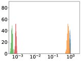
(a) High coherence ${\mathbf{V}}_{k}$.

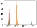
(b) Low coherence ${\mathbf{V}}_{k}$.

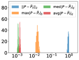
(c) Random ${\mathbf{V}}_{k}$.

Figure 9: Subspace approximation errors produced by RSVD and the maximum, median, and average element-wise error $|({\mathbf{P}}-\widehat{{\mathbf{P}}})_{ij}|$ across $T=250$ trials. The experiment was run with approximation rank $k=70$ (for which $\gamma_{k}\approx 0.853$ and $r_{k}\approx 254.020$), no power iteration ($q=0$), oversampling parameter $p=5$, and varying levels of coherence in ${\mathbf{V}}_{k}$, the true right singular subspace of the $1024\times 1024$ input matrix ${\mathbf{A}}$.

These experiments illustrate two distinct behaviors across difference subspace structure. For both low coherence and random right singular subspaces, the average, median, and maximum element-wise error are all orders of magnitude smaller than the subspace error as seen in Fig. 9(b) and Fig. 9(c). Therefore, for matrices with with incoherent and random right singular subspaces we hypothesize that large $\theta_{\mathrm{max}}$ does not significantly affect the suitability of the approximation to be used in RGKS. In contrast, for coherent subspaces (see Fig. 9(a)), the largest element-wise errors approach the same magnitude as the subspace errors. Nevertheless, the median and average element-wise errors are relatively small. Our hypothesis is that the largest of these element-wise errors occur along the diagonal of the projectors, corresponding to the leverage scores of ${\mathcal{V}}_{k}$ and $\widehat{{\mathcal{V}}}_{k}$. Note that for the highly coherent subspaces we constructed, the leverage score distribution of ${\mathcal{V}}_{k}$ is mostly concentrated in a set of only $k$ indices, making it almost certain that these indices will be selected as skeleton columns even in the presence of noise.

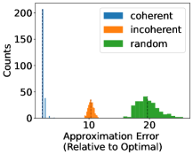
Figure 10: Histogram of RGKS approximation error relative to optimal. For right singular subspaces of the input matrix with varying levels of coherence, rank $k=70$ approximations were computed using oversampling $p=5$ and no power iteraton ($q=0$) across $T=250$ trials. The dashed lines represent the approximation error relative to the optimal when the deterministic GKS algorithm is used.

Complementing our look at subspace perturbations, Fig. 10 shows the approximation error between the input matrix and the RGKS approximation relative to the optimal solution. This error is computed for the same right singular subspaces as Fig. 9. For the coherent case, the approximation error is near the optimal value as well as the error that the deterministic GKS algorithm produces, despite the large element-wise errors seen in Fig. 9(a). In the incoherent and random cases, the RGKS error is distributed around the deterministic GKS error value, demonstrating that the error of the randomized version of the algorithm are not entirely one-sided.

8 Conclusions

We have showed how the accuracy of interpolative decomposition algorithms is affected by the properties of the input matrix being operated on, particularly with respect to singular value decay and singular subspace geometry. Motivated by these considerations, we introduced the RGKS algorithm, a novel interpolative decomposition which uses a randomized approximation of a singular subspace. Numerical experiments in Section 5 showcased the myriad ways in which these interpolative decompositions are affected by singular value decay and singular subspace geometry, and simultaneously, demonstrated that RGKS was competitive with well-known algorithms for low-rank approximation. Surprisingly, these experiments showed that RGKS computed more accurate approximations than RSVD under certain circumstances. Section 6 presented error bounds which described the effects of input matrix structures on a generic interpolative decomposition, and Section 7 specialized these error bounds to RGKS, as well as its deterministic counterpart GKS. In relating the GKS analysis to RGKS, we provided an analysis of randomization errors, while also finding that RGKS exhibits robustness to randomization noise which is difficult to explain with theory alone. We concluded with numerical experiments that shed light on the source of this robustness.

9 Acknowledgements

RA and AD were partially supported by the National Science Foundation under award DMS-2146079. AD was also partially supported by the SciAI Center, funded by the Office of Naval Research (ONR) under Grant Number N00014-23-1-2729.

Appendix A Proofs

A.1 Proof of Conditioning-Based Error Bound

Let ${\mathcal{W}}\subseteq{\mathbb{R}}^{m}$ be a subspace with $\dim{\mathcal{W}}<m$, and let ${\mathbf{P}}_{\mathcal{W}}$ be the orthogonal projector onto ${\mathcal{W}}$. Theorem 6.7 states that if ${\mathbf{E}}={\mathbf{A}}-{\mathbf{P}}_{\mathcal{W}}{\mathbf{A}}$ and $\sigma_{k+1}({\mathbf{E}})>0$, then

$$\|{\mathbf{E}}\|_{2}\leq\|{\mathbf{\Sigma}}_{\perp}\|_{2}\kappa({\mathbf{E}},\,k+1),$$

where $\kappa({\mathbf{E}},\,k+1)=\sigma_{1}({\mathbf{E}})/\sigma_{k+1}({\mathbf{E}})$ is a modified condition number. The proof uses an Ostrowsky-type singular value bound [22, Theorem 6.1], which lets us write

$$\sigma_{k+1}({\mathbf{E}})=\sigma_{k+1}(({\mathbf{I}}-{\mathbf{P}}_{\mathcal{W}}){\mathbf{A}})\leq\sigma_{k+1}({\mathbf{A}})\sigma_{1}({\mathbf{I}}-{\mathbf{P}}_{\mathcal{W}})=\|{\mathbf{\Sigma}}_{\perp}\|_{2}\|{\mathbf{I}}-{\mathbf{P}}_{\mathcal{W}}\|_{2}.$$

Since ${\mathbf{I}}-{\mathbf{P}}_{\mathcal{W}}$ is the orthogonal projector onto ${\mathcal{W}}^{\perp}$, the assumption that $\dim{\mathcal{W}}<m$ implies $\|{\mathbf{I}}-{\mathbf{P}}_{\mathcal{W}}\|_{2}=1$. Thus $\sigma_{k+1}({\mathbf{E}})\leq\|{\mathbf{\Sigma}}_{\perp}\|_{2}$, and since $\|{\mathbf{\Sigma}}_{\perp}\|_{2}=\sigma_{k+1}({\mathbf{A}})>0$, this implies

$$\|{\mathbf{E}}\|_{2}=\|{\mathbf{\Sigma}}_{\perp}\|_{2}\frac{\sigma_{1}({\mathbf{E}})}{\|{\mathbf{\Sigma}}_{\perp}\|_{2}}\leq\|{\mathbf{\Sigma}}_{\perp}\|_{2}\frac{\sigma_{1}({\mathbf{E}})}{\sigma_{k+1}({\mathbf{E}})}=\|{\mathbf{\Sigma}}_{\perp}\|_{2}\kappa({\mathbf{E}},\,k+1),$$

as desired.

A.2 Proof of Residual Singular Value Inequality

Using the notation of the previous proof, Lemma 6.9 states that $\sigma_{i}({\mathbf{E}})\geq\sigma_{k+i}({\mathbf{A}})$ for $1\leq i\leq\min\{m,\,n\}-k$. To show this, write ${\mathbf{E}}={\mathbf{E}}_{i-1}+{\mathbf{F}}_{i-1}$, where ${\mathbf{E}}_{i-1}$ is an optimal rank-$(i-1)$ approximation of ${\mathbf{E}}$ in the sense of the Eckart-Young theorem, and ${\mathbf{F}}_{i-1}$ is the residual of this approximation. Then $\sigma_{i}({\mathbf{E}})=\|{\mathbf{F}}_{i-1}\|_{2}$. Furthermore, the relations $\operatorname{rank}{\mathbf{P}}_{\mathcal{W}}{\mathbf{A}}\leq k$ and $\operatorname{rank}{\mathbf{E}}_{i-1}\leq i-1$ imply that

(25) $$\operatorname{rank}({\mathbf{P}}_{\mathcal{W}}{\mathbf{A}}+{\mathbf{E}}_{i-1})\leq k+i-1.$$

By Weyl’s inequality,

$$\sigma_{k+i}({\mathbf{A}}) =\sigma_{k+i}({\mathbf{P}}_{\mathcal{W}}{\mathbf{A}}+{\mathbf{E}}_{i-1}+{\mathbf{F}}_{i-1})$$

$$\leq\sigma_{k+i}({\mathbf{P}}_{\mathcal{W}}{\mathbf{A}}+{\mathbf{E}}_{i-1})+\|{\mathbf{F}}_{i-1}\|_{2}$$

$$=\sigma_{k+i}({\mathbf{P}}_{\mathcal{W}}{\mathbf{A}}+{\mathbf{E}}_{i-1})+\sigma_{i}({\mathbf{E}}).$$

Equation Eq. 25 shows that $\sigma_{k+i}({\mathbf{P}}_{\mathcal{W}}{\mathbf{A}}+{\mathbf{E}}_{i-1})=0$, completing the proof.

A.3 Review of Principal Angles and the CS Decomposition

Several of the results in this paper concern angles between subspaces and we use this section to briefly review the theory of principal angles. If ${\mathcal{X}}$ and ${\mathcal{Y}}$ are 1-dimensional subspaces of ${\mathbb{R}}^{n}$ spanned by unit vectors ${\mathbf{x}}$ and ${\mathbf{y}}$, then the principal angle between ${\mathcal{X}}$ and ${\mathcal{Y}}$ is the number $\theta\in[0,\,\pi/2]$ defined in the usual geometric sense, $\cos\theta=|{\mathbf{x}}^{\mathrm{T}}{\mathbf{y}}|$. More generally, if ${\mathcal{X}}$ and ${\mathcal{Y}}$ are $k$-dimensional subspaces of ${\mathbb{R}}^{n}$ with $k>1$, then the principal angles between ${\mathcal{X}}$ and ${\mathcal{Y}}$ are the the numbers $\theta_{1},\,\ldots,\,\theta_{k}\in[0,\,\pi/2]$ defined by

$$\cos\theta_{i}=|{\mathbf{x}}_{i}^{\mathrm{T}}{\mathbf{y}}_{i}|,$$

where ${\mathbf{x}}_{1},\,\ldots,\,{\mathbf{x}}_{k}\in{\mathcal{X}}$ and ${\mathbf{y}}_{1},\,\ldots,\,{\mathbf{y}}_{k}\in{\mathcal{Y}}$ are defined recursively by

$${\mathbf{x}}_{1}^{\mathrm{T}}{\mathbf{y}}_{1} =\max_{\begin{subarray}{c}{\mathbf{x}}\in{\mathcal{X}},\,\|{\mathbf{x}}\|_{2}=1\\ {\mathbf{y}}\in{\mathcal{Y}},\,\|{\mathbf{y}}\|_{2}=1\end{subarray}}|{\mathbf{x}}^{\mathrm{T}}{\mathbf{y}}|$$

$${\mathbf{x}}_{i+1}^{\mathrm{T}}{\mathbf{y}}_{i+1} =\max_{\begin{subarray}{c}{\mathbf{x}}\in{\mathcal{X}},\,\|{\mathbf{x}}\|_{2}=1\\ {\mathbf{x}}^{\mathrm{T}}[{\mathbf{x}}_{1},\,\ldots,\,{\mathbf{x}}_{i}]={\mathbf{0}}\end{subarray}}\left(\max_{\begin{subarray}{c}{\mathbf{y}}\in{\mathcal{Y}},\,\|{\mathbf{y}}\|_{2}=1\\ {\mathbf{y}}^{\mathrm{T}}[{\mathbf{y}}_{1},\,\ldots,\,{\mathbf{y}}_{i}]={\mathbf{0}}\end{subarray}}|{\mathbf{x}}^{\mathrm{T}}{\mathbf{y}}|\right)\quad\text{for }1\leq i<k.$$

A consequence of this definition is that $\theta_{1}\leq\theta_{2}\ldots\leq\theta_{k}$.

Given concrete representations of ${\mathcal{X}}$ and ${\mathcal{Y}}$ in the form of two orthonormal bases, one can compute the angles $\theta_{i}$ and the vectors ${\mathbf{x}}_{i},\,{\mathbf{y}}_{i}$ using an SVD. Specifically, let ${\mathbf{X}},\,{\mathbf{Y}}\in{\mathbb{R}}^{n\times k}$ be orthonormal bases for ${\mathcal{X}}$ and ${\mathcal{Y}}$, respectively, and consider the singular value decomposition ${\mathbf{X}}^{\mathrm{T}}{\mathbf{Y}}={\mathbf{U}}{\mathbf{C}}{\mathbf{V}}^{\mathrm{T}}$, where ${\mathbf{U}}$ and ${\mathbf{V}}$ are orthogonal, and ${\mathbf{C}}=\mathrm{diag}(c_{1},\,\ldots,\,c_{k})$ with $c_{1}\geq\ldots\geq c_{k}\geq 0$. This decomposition reveals the principal angles and vectors through the identities

$$c_{i}=\cos\theta_{i},\quad{\mathbf{X}}{\mathbf{U}}=\begin{bmatrix}{\mathbf{x}}_{1}&\cdots&{\mathbf{x}}_{k}\end{bmatrix},\quad{\mathbf{Y}}{\mathbf{V}}=\begin{bmatrix}{\mathbf{y}}_{1}&\cdots&{\mathbf{y}}_{k}\end{bmatrix},$$

as discussed in [17, section 6.4.3].

Principal angles and vectors can be represented in a more comprehensive way using a CS decomposition. Given an orthogonal matrix ${\mathbf{Q}}\in{\mathbb{R}}^{n\times n}$ and an integer $k\leq n/2$, the CS decomposition of ${\mathbf{Q}}$ is ${\mathbf{Q}}={\mathbf{U}}{\mathbf{T}}{\mathbf{V}}^{\mathrm{T}}$, where

$${\mathbf{U}}=\bNiceMatrix[last-row,last-col]{\mathbf{U}}_{1}&\mathbf{0}\mbox{\scriptsize$k$}\\ \mathbf{0}{\mathbf{U}}_{2}\mbox{\scriptsize$n-k$}\\ \mbox{\scriptsize$k$}\mbox{\scriptsize$n-k$}\,,\quad{\mathbf{T}}=\bNiceMatrix[last-row,last-col]{\mathbf{C}}&{\mathbf{S}}\mathbf{0}\mbox{\scriptsize$k$}\\ {\mathbf{S}}-{\mathbf{C}}\mathbf{0}\mbox{\scriptsize$k$}\\ \mathbf{0}\mathbf{0}{\mathbf{I}}\mbox{\scriptsize$n-2k$}\\ \mbox{\scriptsize$k$}\mbox{\scriptsize$k$}\mbox{\scriptsize$n-2k$}\,,\quad{\mathbf{V}}=\bNiceMatrix[last-row,last-col]{\mathbf{V}}_{1}&\mathbf{0}\mbox{\scriptsize$k$}\\ \mathbf{0}{\mathbf{V}}_{2}\mbox{\scriptsize$n-k$}\\ \mbox{\scriptsize$k$}\mbox{\scriptsize$n-k$}\,.$$

Here, ${\mathbf{U}}_{1},\,{\mathbf{U}}_{2},\,{\mathbf{V}}_{1},\,{\mathbf{V}}_{2}$ are orthogonal matrices, while ${\mathbf{C}}$ and ${\mathbf{S}}$ are diagonal matrices with nonnegative entries, satisfying ${\mathbf{C}}^{2}+{\mathbf{S}}^{2}={\mathbf{I}}$. Such a decomposition exists for any orthogonal ${\mathbf{Q}}$ [17]. The connection to principal angles is as follows: let ${\mathcal{X}},\,{\mathcal{Y}}\subseteq{\mathbb{R}}^{n}$ be $k$-dimensional subspaces with orthonormal bases ${\mathbf{X}}$ and ${\mathbf{Y}}$, and similarly, let ${\mathbf{X}}_{\perp}$ and ${\mathbf{Y}}_{\perp}$ be orthonormal bases for ${\mathcal{X}}^{\perp}$ and ${\mathcal{Y}}^{\perp}$. Then, the matrix

$${\mathbf{Q}}=\begin{bmatrix}{\mathbf{X}}^{\mathrm{T}}{\mathbf{Y}}&{\mathbf{X}}^{\mathrm{T}}{\mathbf{Y}}_{\perp}\\ {\mathbf{X}}_{\perp}^{\mathrm{T}}{\mathbf{Y}}&{\mathbf{X}}_{\perp}^{\mathrm{T}}{\mathbf{Y}}_{\perp}\end{bmatrix}$$

is orthogonal. If ${\mathbf{C}}$ and ${\mathbf{S}}$ are the diagonal factors resulting from a CS decomposition of ${\mathbf{Q}}$, then ${\mathbf{C}}=\mathrm{diag}(\cos\theta_{1},\,\ldots,\,\cos\theta_{k})$ and ${\mathbf{S}}=\mathrm{diag}(\sin\theta_{1},\,\ldots,\,\sin\theta_{k})$, where $\theta_{1},\,\ldots,\,\theta_{k}$ are the principal angles between ${\mathcal{X}}$ and ${\mathcal{Y}}$.

A.4 Proof of Principal Angle Lemma

Let ${\mathbf{A}}$ be an $m\times n$ matrix and let ${\mathbf{A}}={\mathbf{U}}_{k}{\mathbf{\Sigma}}_{k}{\mathbf{V}}_{k}^{\mathrm{T}}+{\mathbf{U}}_{\perp}{\mathbf{\Sigma}}_{\perp}{\mathbf{V}}_{\perp}^{\mathrm{T}}$ be an SVD partitioned at rank $k$, chosen such that $\sigma_{k}({\mathbf{A}})>\sigma_{k+1}({\mathbf{A}})$. To allow the use of the CS decomposition, we impose the restriction that $k\leq n/2$. Given a selection $J=\{j_{1},\,\ldots,\,j_{k}\}$ of column indices, let $\varphi_{1},\,\ldots,\,\varphi_{k}$ be the principal angles between ${\mathcal{I}}_{J}=\operatorname{range}({\mathbf{I}}_{:,\,J})$ and ${\mathcal{V}}_{k}=\operatorname{range}({\mathbf{V}}_{k})$. The first claim of Lemma 6.3 is that $\cos\varphi_{1},\,\ldots,\,\cos\varphi_{k}$ are the singular values of ${\mathbf{V}}_{J,\,1:k}$. This follows from the fact that ${\mathbf{I}}_{:,\,J}$ and ${\mathbf{V}}_{k}$ are orthonormal bases for ${\mathcal{I}}_{J}$ and ${\mathcal{V}}_{k}$, and that ${\mathbf{V}}_{J,\,1:k}=({\mathbf{I}}_{:,\,J})^{\mathrm{T}}{\mathbf{V}}_{k}$. We now have that $\sigma_{\mathrm{min}}({\mathbf{V}}_{:,\,1:k})=\cos\varphi_{\mathrm{max}}$, which implies that ${\mathbf{V}}_{:,\,1:k}$ is invertible if and only if $\varphi_{\mathrm{max}}<\pi/2$. This proves the second claim of Lemma 6.3.

The final claim of Lemma 6.3 is that the singular values of ${\mathbf{V}}_{[n]\setminus J,\,1:k}({\mathbf{V}}_{J,\,1:k})^{-1}$ are equal to $\tan\varphi_{1},\,\ldots,\,\tan\varphi_{k}$, provided ${\mathbf{V}}_{J,\,1:k}$ is invertible. Let ${\mathbf{V}}=[{\mathbf{V}}_{k}\>\>{\mathbf{V}}_{\perp}]$, and consider a CS decomposition of $\mathbf{{\Pi}}^{\mathrm{T}}{\mathbf{V}}$:

$$\begin{bmatrix}{\mathbf{V}}_{J,\,1:k}&{\mathbf{V}}_{J,\,k+1:n}\\ {\mathbf{V}}_{[n]\setminus J,\,1:k}&{\mathbf{V}}_{[n]\setminus J,\,k+1:n}\end{bmatrix}=\begin{bmatrix}{\mathbf{Q}}_{1}{\mathbf{C}}{\mathbf{W}}_{1}^{\mathrm{T}}&{\mathbf{Q}}_{1}\begin{bmatrix}{\mathbf{S}}&\mathbf{0}\end{bmatrix}{\mathbf{W}}_{2}^{\mathrm{T}}\\ {\mathbf{Q}}_{2}\begin{bmatrix}{\mathbf{S}}\\ \mathbf{0}\end{bmatrix}{\mathbf{W}}_{1}^{\mathrm{T}}&{\mathbf{Q}}_{2}\begin{bmatrix}-{\mathbf{C}}&\mathbf{0}\\ \mathbf{0}&{\mathbf{I}}\end{bmatrix}{\mathbf{W}}_{2}^{\mathrm{T}}\end{bmatrix},$$

where ${\mathbf{Q}}_{1},\,{\mathbf{W}}_{1}\in{\mathbb{R}}^{k\times k}$ and ${\mathbf{Q}}_{2},\,{\mathbf{W}}_{2}\in{\mathbb{R}}^{(n-k)\times(n-k)}$ are orthogonal matrices, ${\mathbf{C}}=\mathrm{diag}(\cos\varphi_{1},\,\ldots,\,\cos\varphi_{k})$, and ${\mathbf{S}}=\mathrm{diag}(\sin\varphi_{1},\,\ldots,\,\sin\varphi_{k})$. The claim then follows from the relation

$${\mathbf{V}}_{[n]\setminus J,\,1:k}({\mathbf{V}}_{J,\,1:k})^{-1}={\mathbf{Q}}_{2}\begin{bmatrix}{\mathbf{S}}{\mathbf{C}}^{-1}\\ \mathbf{0}\end{bmatrix}{\mathbf{Q}}_{1}^{\mathrm{T}},$$

where ${\mathbf{S}}{\mathbf{C}}^{-1}=\mathrm{diag}(\tan\varphi_{1},\,\ldots,\,\tan\varphi_{k})$. Note that $({\mathbf{V}}_{J,\,1:k})^{-1}{\mathbf{V}}_{J,\,k+1:n}$ also has singular values equal to $\tan\varphi_{1},\,\ldots,\,\varphi_{n}$, since

(26) $$({\mathbf{V}}_{J,\,1:k})^{-1}{\mathbf{V}}_{J,\,k+1:n}={\mathbf{W}}_{1}\begin{bmatrix}{\mathbf{C}}^{-1}{\mathbf{S}}&\mathbf{0}\end{bmatrix}{\mathbf{W}}_{2}^{\mathrm{T}}.$$

A.5 Review of Sketching Algorithm Analysis

Our proofs of Theorem 6.1 and Theorem 6.5 will rely on an inequality originally used for the analysis of sketching algorithms, which we review here for completeness. The inequality is due to Halko, Martinsson, and Tropp [19], and pertains to the “sketching proto algorithm” for computing a rank-$k$ approximation ${\mathbf{A}}\approx{\mathbf{B}}_{1}{\mathbf{B}}_{2}^{\mathrm{T}}$ [19, Algorithm 4.1], which we summarize as Algorithm 3.

Algorithm 3 Sketching Proto-Algorithm

1:  Generate a matrix ${\mathbf{\Omega}}$ of size $n\times k$.

2:  Compute a thin QR factorization ${\mathbf{A}}{\mathbf{\Omega}}={\mathbf{Q}}{\mathbf{R}}$.

3:  return  ${\mathbf{B}}_{1}={\mathbf{Q}},\,{\mathbf{B}}_{2}={\mathbf{A}}^{\mathrm{T}}{\mathbf{Q}}$.

Although ${\mathbf{\Omega}}$ is, in practice, drawn from a carefully chosen random distribution, Halko et al. provide a deterministic error bound for Algorithm 3 which considers ${\mathbf{\Omega}}$ to be any arbitrary fixed matrix. We are referring to [19, Theorem 9.1], which we state below as Lemma A.1.

Lemma A.1 (Halko, Martinsson, and Tropp, 2011).

Given an $m\times n$ matrix ${\mathbf{A}}$ and an approximation rank $k\leq\min\{m,\,n\}$, consider the singular value decomposition ${\mathbf{A}}={\mathbf{U}}_{k}{\mathbf{\Sigma}}_{k}{\mathbf{V}}_{k}^{\mathrm{T}}+{\mathbf{U}}_{\perp}{\mathbf{\Sigma}}_{\perp}{\mathbf{V}}_{\perp}^{\mathrm{T}}$ partitioned at rank $k$. Let ${\mathbf{\Omega}}$ be the matrix in line 1 of Algorithm 3, and let

$${\mathbf{\Omega}}_{1}={\mathbf{V}}_{k}^{\mathrm{T}}{\mathbf{\Omega}},\qquad{\mathbf{\Omega}}_{2}={\mathbf{V}}_{\perp}^{\mathrm{T}}{\mathbf{\Omega}},$$

be matrices that describe the correlation between ${\mathbf{\Omega}}$ and the right singular subspaces of ${\mathbf{A}}$. If ${\mathbf{B}}_{1}\in{\mathbb{R}}^{m\times k}$ and ${\mathbf{B}}_{2}\in{\mathbb{R}}^{n\times k}$ are the output of Algorithm 3, then provided that ${\mathbf{\Omega}}_{1}$ is full-rank,

$$\|{\mathbf{A}}-{\mathbf{B}}_{1}{\mathbf{B}}_{2}^{\mathrm{T}}\|^{2}\leq\|{\mathbf{\Sigma}}_{\perp}\|^{2}+\|{\mathbf{\Sigma}}_{\perp}{\mathbf{\Omega}}_{1}{\mathbf{\Omega}}_{2}^{\dagger}\|^{2},$$

where $\|\cdot\|$ is either the spectral or Frobenius norm.

A.6 Proof of Spectral Norm Subspace Geometry Bound

Theorem 6.1 states that if $\varphi_{\mathrm{max}}<\pi/2$, then

$$\|{\mathbf{A}}-{\mathbf{A}}_{:,\,J}({\mathbf{A}}_{:,\,J})^{\dagger}{\mathbf{A}}\|_{2}\leq\|{\mathbf{\Sigma}}_{\perp}\|_{2}\sec\varphi_{\mathrm{max}}.$$

To prove this inequality, let $\mathbf{{\Pi}}$ be a permutation which moves indices $J$ to the front (i.e., $\mathbf{{\Pi}}=\begin{bmatrix}{\mathbf{I}}_{:,\,J}&{\mathbf{I}}_{:,\,[n]\setminus J}\end{bmatrix}$). Let ${\mathbf{V}}=[{\mathbf{V}}_{k}\>\>{\mathbf{V}}_{\perp}]$, and partition $\mathbf{{\Pi}}^{\mathrm{T}}{\mathbf{V}}$ as

(27) $$\mathbf{{\Pi}}^{\mathrm{T}}{\mathbf{V}}=\bNiceMatrix[last-row,last-col]{\mathbf{V}}_{11}&{\mathbf{V}}_{12}\mbox{\scriptsize$k$}\\ {\mathbf{V}}_{21}{\mathbf{V}}_{22}\mbox{\scriptsize$n-k$}\\ \mbox{\scriptsize$k$}\mbox{\scriptsize$n-k$}\,.$$

The matrix of skeleton columns is ${\mathbf{A}}_{:,\,J}={\mathbf{A}}(\mathbf{{\Pi}}_{:,\,1:k})$, and if ${\mathbf{A}}(\mathbf{{\Pi}}_{:,\,1:k})={\mathbf{Q}}{\mathbf{R}}$ is a thin QR factorization, then ${\mathbf{A}}_{:,\,J}({\mathbf{A}}_{:,\,J})^{\dagger}{\mathbf{A}}={\mathbf{Q}}{\mathbf{Q}}^{\mathrm{T}}{\mathbf{A}}={\mathbf{B}}_{1}{\mathbf{B}}_{2}^{\mathrm{T}}$, with ${\mathbf{B}}_{1}={\mathbf{Q}}$ and ${\mathbf{B}}_{2}={\mathbf{A}}^{\mathrm{T}}{\mathbf{Q}}$. This construction of ${\mathbf{A}}_{:,\,J}({\mathbf{A}}_{:,\,J})^{\dagger}{\mathbf{A}}$ is equivalent to running Algorithm 3 on ${\mathbf{A}}$, using ${\mathbf{\Omega}}=\mathbf{{\Pi}}_{:,\,1:k}$ as the matrix in line 1. Therefore, letting ${\mathbf{\Omega}}_{1}={\mathbf{V}}_{k}^{\mathrm{T}}{\mathbf{\Omega}}$ and ${\mathbf{\Omega}}_{2}={\mathbf{V}}_{\perp}^{\mathrm{T}}{\mathbf{\Omega}}$, we apply the inequality of Halko, Martinsson, and Tropp (Lemma A.1) to see that

(28) $$\|{\mathbf{A}}-{\mathbf{A}}_{:,\,J}({\mathbf{A}}_{:,\,J})^{\dagger}{\mathbf{A}}\|^{2}\leq\|{\mathbf{\Sigma}}_{\perp}\|^{2}+\|{\mathbf{\Sigma}}_{\perp}{\mathbf{\Omega}}_{2}{\mathbf{\Omega}}_{1}^{\dagger}\|^{2},$$

where $\|\cdot\|$ is the spectral or Frobenius norm, provided that ${\mathbf{\Omega}}_{1}$ is full-rank. Our specific choice of ${\mathbf{\Omega}}$ implies that

$${\mathbf{\Omega}}_{1}^{\mathrm{T}}=(\mathbf{{\Pi}}_{:,\,1:k})^{\mathrm{T}}{\mathbf{V}}_{k}={\mathbf{V}}_{11},\qquad{\mathbf{\Omega}}_{2}^{\mathrm{T}}=(\mathbf{{\Pi}}_{:,\,1:k})^{\mathrm{T}}{\mathbf{V}}_{\perp}={\mathbf{V}}_{12}.$$

Furthermore, the relation ${\mathbf{\Omega}}_{1}^{\mathrm{T}}=({\mathbf{I}}_{:,\,J})^{\mathrm{T}}{\mathbf{V}}_{k}={\mathbf{V}}_{J,\,1:k}$ implies by Lemma 6.3 that $\sigma_{\mathrm{min}}({\mathbf{\Omega}}_{1})=\cos\varphi_{\mathrm{max}}$. Therefore, ${\mathbf{\Omega}}_{1}$ is full-rank if and only if $\varphi_{\mathrm{max}}<\pi/2$, in which case Eq. 28 becomes $\|{\mathbf{A}}-{\mathbf{A}}_{:,\,J}({\mathbf{A}}_{:,\,J})^{\dagger}{\mathbf{A}}\|^{2}\leq\|{\mathbf{\Sigma}}_{\perp}\|^{2}+\|{\mathbf{\Sigma}}_{\perp}{\mathbf{V}}_{12}^{\mathrm{T}}{\mathbf{V}}_{11}^{-\mathrm{T}}\|^{2}$. Because the inequality $\|{\mathbf{X}}{\mathbf{Y}}\|\leq\|{\mathbf{X}}\|_{2}\|{\mathbf{Y}}\|$ holds in both the spectral and Frobenius norm, we obtain

(29) $$\|{\mathbf{A}}-{\mathbf{A}}_{:,\,J}({\mathbf{A}}_{:,\,J})^{\dagger}{\mathbf{A}}\|^{2}\leq\|{\mathbf{\Sigma}}_{\perp}\|^{2}+\|{\mathbf{\Sigma}}_{\perp}\|_{2}^{2}\|{\mathbf{V}}_{11}^{-1}{\mathbf{V}}_{12}\|^{2}.$$

Equation Eq. 26 shows that the singular values of ${\mathbf{V}}_{11}^{-1}{\mathbf{V}}_{12}=({\mathbf{V}}_{J,\,1:k})^{-1}{\mathbf{V}}_{J,\,k+1:n}$ are equal to $\tan\varphi_{1},\,\ldots,\,\tan\varphi_{k}$. The spectral norm of ${\mathbf{V}}_{11}^{-1}{\mathbf{V}}_{12}$ is therefore $\tan\varphi_{\mathrm{max}}$, meaning that

$$\|{\mathbf{A}}-{\mathbf{A}}_{:,\,J}({\mathbf{A}}_{:,\,J})^{\dagger}{\mathbf{A}}\|_{2}^{2}\leq\|{\mathbf{\Sigma}}_{\perp}\|_{2}^{2}(1+\tan^{2}\varphi_{\mathrm{max}})=\|{\mathbf{\Sigma}}_{\perp}\|_{2}^{2}\sec^{2}\varphi_{\mathrm{max}},$$

which completes the proof.

A.7 Proof of Frobenius Norm Subspace Geometry Bound

Theorem 6.5 that if $\varphi_{\mathrm{max}}\leq\pi/2$, then

$$\|{\mathbf{A}}-{\mathbf{A}}_{:,\,J}({\mathbf{A}}_{:,\,J})^{\dagger}{\mathbf{A}}\|_{\mathrm{F}}\leq\|{\mathbf{\Sigma}}_{\perp}\|_{\mathrm{F}}\sqrt{1+\frac{1}{r_{k}}\sum_{i=1}^{k}\tan^{2}\varphi_{i}},$$

where $r_{k}=\|{\mathbf{\Sigma}}_{\perp}\|_{\mathrm{F}}^{2}/\|{\mathbf{\Sigma}}_{\perp}\|_{2}^{2}$ is the residual stable rank. We start with equation Eq. 29, which, when written in the Frobenius norm, becomes

$$\|{\mathbf{A}}-{\mathbf{A}}_{:,\,J}({\mathbf{A}}_{:,\,J})^{\dagger}{\mathbf{A}}\|_{\mathrm{F}}^{2}\leq\|{\mathbf{\Sigma}}_{\perp}\|_{\mathrm{F}}^{2}+\frac{\|{\mathbf{\Sigma}}_{\perp}\|_{\mathrm{F}}^{2}}{r_{k}}\|{\mathbf{V}}_{11}^{-1}{\mathbf{V}}_{12}\|_{\mathrm{F}}^{2}.$$

As before, we use Eq. 26 to expand $\|{\mathbf{V}}_{11}^{-1}{\mathbf{V}}_{12}\|_{\mathrm{F}}$ in terms of $\tan\varphi_{1},\,\ldots,\,\tan\varphi_{k}$, after which the proof is complete.

A.8 Proof of Full Subspace Perturbation Bound

We now introduce $\widehat{{\mathcal{V}}}_{k}$, the $k$-dimensional subspace of ${\mathbb{R}}^{n}$ spanned by the approximate right singular vectors computed by RSVD in line 1 of RGKS (Algorithm 2). Theorem 7.1 states that

(30) $$\varphi_{\mathrm{max}}\leq\widehat{\varphi}_{\mathrm{max}}+\theta_{\mathrm{max}},$$

where $\theta_{\mathrm{max}}$ is the largest principal angle between ${\mathcal{V}}_{k}$ and $\widehat{{\mathcal{V}}}_{k}$, and $\widehat{\varphi}_{\mathrm{max}}$ is the largest principal angle between $\widehat{{\mathcal{V}}}_{k}$ and ${\mathcal{I}}_{J}$. Equation Eq. 30 is a special case of the triangle inequalities proven in [25] for symmetric gauge functions over principal angles, if one takes the gauge function to be the supremum norm. Here we will offer a more elementary proof using basic singular value inequalities. Because the cosine function is strictly decreasing on $[0,\,\pi]$, Eq. 30 is equivalent to

$$\cos\varphi_{\mathrm{max}}\geq\cos(\widehat{\varphi}_{\mathrm{max}}+\theta_{\mathrm{max}}),$$

which is what we will prove instead. As discussed in the proof of Lemma 6.3, $\cos\varphi_{\mathrm{max}}=\sigma_{\mathrm{min}}({\mathbf{V}}_{J,\,1:k})=\sigma_{\mathrm{min}}({\mathbf{V}}_{11})$, following the partition of $\mathbf{{\Pi}}^{\mathrm{T}}{\mathbf{V}}$ given in Eq. 27. Similarly, letting $\widehat{{\mathbf{V}}}_{k}\in{\mathbb{R}}^{n\times k}$ and $\widehat{{\mathbf{V}}}_{\perp}\in{\mathbb{R}}^{n\times(n-k)}$ be orthonormal bases for $\widehat{{\mathcal{V}}}_{k}$ and $\widehat{{\mathcal{V}}}_{k}^{\perp}$, the partitioning

$$\mathbf{{\Pi}}^{\mathrm{T}}\begin{bmatrix}\widehat{{\mathbf{V}}}_{k}&\widehat{{\mathbf{V}}}_{\perp}\end{bmatrix}=\bNiceMatrix[last-row,last-col]\widehat{{\mathbf{V}}}_{11}&\widehat{{\mathbf{V}}}_{12}\mbox{\scriptsize$k$}\\ \widehat{{\mathbf{V}}}_{21}\widehat{{\mathbf{V}}}_{22}\mbox{\scriptsize$n-k$}\\ \mbox{\scriptsize$k$}\mbox{\scriptsize$n-k$}$$

implies $\cos\widehat{\varphi}_{\mathrm{max}}=\sigma_{\mathrm{min}}(\widehat{{\mathbf{V}}}_{11})$. Let $\widehat{{\mathbf{V}}}=[\widehat{{\mathbf{V}}}_{k}\>\>\widehat{{\mathbf{V}}}_{\perp}]$, and consider the CS decomposition

$$\widehat{{\mathbf{V}}}^{\mathrm{T}}{\mathbf{V}}=\begin{bmatrix}{\mathbf{Q}}_{1}{\mathbf{C}}{\mathbf{W}}_{1}^{\mathrm{T}}&{\mathbf{Q}}_{1}\begin{bmatrix}{\mathbf{S}}&\mathbf{0}\end{bmatrix}{\mathbf{W}}_{2}^{\mathrm{T}}\\ {\mathbf{Q}}_{2}\begin{bmatrix}{\mathbf{S}}\\ \mathbf{0}\end{bmatrix}{\mathbf{W}}_{1}^{\mathrm{T}}&{\mathbf{Q}}_{2}\begin{bmatrix}-{\mathbf{C}}&\mathbf{0}\\ \mathbf{0}&{\mathbf{I}}\end{bmatrix}{\mathbf{W}}_{2}^{\mathrm{T}}\end{bmatrix},$$

where ${\mathbf{Q}}_{1},\,{\mathbf{W}}_{1}\in{\mathbb{R}}^{k\times k}$ and ${\mathbf{Q}}_{2},\,{\mathbf{W}}_{2}\in{\mathbb{R}}^{(n-k)\times(n-k)}$ are orthogonal matrices, ${\mathbf{C}}=\mathrm{diag}(\cos\theta_{1},\,\ldots,\,\cos\theta_{k})$, ${\mathbf{S}}=\mathrm{diag}(\sin\theta_{1},\,\ldots,\,\sin\theta_{k})$, and $\theta_{1},\,\ldots,\,\theta_{k}$ are the principal angles between ${\mathcal{V}}_{k}$ and $\widehat{{\mathcal{V}}}_{k}$. Using this decomposition, we write

$${\mathbf{V}}_{k}=\widehat{{\mathbf{V}}}(\widehat{{\mathbf{V}}}^{\mathrm{T}}{\mathbf{V}})_{:,\,1:k}=\widehat{{\mathbf{V}}}_{k}{\mathbf{Q}}_{1}{\mathbf{C}}{\mathbf{W}}_{1}^{\mathrm{T}}+\widehat{{\mathbf{V}}}_{\perp}{\mathbf{Q}}_{2}{\mathbf{\Psi}}{\mathbf{W}}_{1}^{\mathrm{T}},$$

where ${\mathbf{\Psi}}=[{\mathbf{S}}\>\>\mathbf{0}]^{\mathrm{T}}$. Then,

$${\mathbf{V}}_{11} =(\mathbf{{\Pi}}_{:,\,1:k})^{\mathrm{T}}{\mathbf{V}}_{k}$$

$$=(\mathbf{{\Pi}}_{:,\,1:k})^{\mathrm{T}}\widehat{{\mathbf{V}}}_{k}{\mathbf{Q}}_{1}{\mathbf{C}}{\mathbf{W}}_{1}^{\mathrm{T}}+(\mathbf{{\Pi}}_{:,\,1:k})^{\mathrm{T}}\widehat{{\mathbf{V}}}_{\perp}{\mathbf{Q}}_{2}{\mathbf{\Psi}}{\mathbf{W}}_{1}^{\mathrm{T}}$$

$$=(\widehat{{\mathbf{V}}}_{11}{\mathbf{Q}}_{1}{\mathbf{C}}+\widehat{{\mathbf{V}}}_{12}{\mathbf{Q}}_{2}{\mathbf{\Psi}}){\mathbf{W}}_{1}^{\mathrm{T}}.$$

We now use the orthogonal invariance of singular values, an Ostrowsky-type bound [22, Theorem 6.1], and Weyl’s inequality to write

$$\cos\varphi_{\mathrm{max}} =\sigma_{\mathrm{min}}({\mathbf{V}}_{11})=\sigma_{\mathrm{min}}(\widehat{{\mathbf{V}}}_{11}{\mathbf{Q}}_{1}{\mathbf{C}}+\widehat{{\mathbf{V}}}_{12}{\mathbf{Q}}_{2}{\mathbf{\Psi}})$$

$$\geq\sigma_{\mathrm{min}}(\widehat{{\mathbf{V}}}_{11})\sigma_{\mathrm{min}}({\mathbf{C}})-\sigma_{\mathrm{max}}(\widehat{{\mathbf{V}}}_{12})\sigma_{\mathrm{max}}({\mathbf{\Psi}})$$

$$=\sigma_{\mathrm{min}}(\widehat{{\mathbf{V}}}_{11})\cos\theta_{\mathrm{max}}-\sigma_{\mathrm{max}}(\widehat{{\mathbf{V}}}_{12})\sin\theta_{\mathrm{max}}.$$

We have already seen that $\sigma_{\mathrm{min}}(\widehat{{\mathbf{V}}}_{11})=\cos\widehat{\varphi}_{\mathrm{max}}$, and a CS decomposition of $\widehat{{\mathbf{V}}}$ reveals that $\sigma_{\mathrm{max}}(\widehat{{\mathbf{V}}}_{12})^{2}=1-\sigma_{\mathrm{min}}(\widehat{{\mathbf{V}}}_{11})^{2}=\sin^{2}\widehat{\varphi}_{\mathrm{max}}$. Therefore,

$$\cos\varphi_{\mathrm{max}}\geq\cos\widehat{\varphi}_{\mathrm{max}}\cos\theta_{\mathrm{max}}-\sin\widehat{\varphi}_{\mathrm{max}}\sin\theta_{\mathrm{max}}=\cos(\widehat{\varphi}_{\mathrm{max}}+\theta_{\mathrm{max}}),$$

which completes the proof.

A.9 Proof of Restricted Subspace Geometry Error Bound

Let $\widehat{{\mathcal{V}}}_{k-t}$ be the subspace spanned by the first $k-t$ right singular vectors estimated in line 1 or RGKS (Algorithm 2), and let $\theta_{\mathrm{max}}^{(k-t)}$ be the largest principal angle between ${\mathcal{V}}_{k-t}$ and $\widehat{{\mathcal{V}}}_{k-t}$. Equation Eq. 22 states that

$$\|{\mathbf{A}}-{\mathbf{A}}_{:,\,J}({\mathbf{A}}_{:,\,J})^{\dagger}{\mathbf{A}}\|_{2}\leq\frac{\|{\mathbf{\Sigma}}_{\perp}\|_{2}}{\gamma_{k-t+1,\,k+1}}\sec(\widehat{\varphi}_{\mathrm{max}}+\theta_{\mathrm{max}}^{(k-t)}).$$

To prove this bound, consider an arbitrary subset $I\subseteq J$ of size $k-t$. We will use equation Eq. 11 to bound the RGKS error in terms of $\varphi_{\mathrm{max}}^{(I)}$, the largest principal angle between ${\mathcal{V}}_{k-t}$ and ${\mathcal{I}}_{I}$. If $\widehat{\varphi}_{\mathrm{max}}^{(I)}$ is the largest angle between $\widehat{{\mathcal{V}}}_{k-t}$ and ${\mathcal{I}}_{I}$, and $\theta_{\mathrm{max}}^{(k-t)}$ is the largest angle between ${\mathcal{V}}_{k-t}$ and $\widehat{{\mathcal{V}}}_{k-t}$, then we have

$$\varphi_{\mathrm{max}}^{(I)}\leq\widehat{\varphi}_{\mathrm{max}}^{(I)}+\theta_{\mathrm{max}}^{(k-t)}\quad\text{and}\quad\widehat{\varphi}_{\mathrm{max}}^{(I)}\leq\widehat{\varphi}_{\mathrm{max}}.$$

The first of these inequalities is a direct consequence of Theorem 7.1. For the second inequality, note that the minimal singular value of a matrix is smaller than that of any of its submatrices. In particular,

$$\cos\widehat{\varphi}_{\mathrm{max}}=\sigma_{\mathrm{min}}({\mathbf{V}}_{J,\,1:k})\leq\sigma_{\mathrm{min}}({\mathbf{V}}_{I,\,1:k-t})=\cos\widehat{\varphi}_{\mathrm{max}}^{(I)},$$

where we have used Lemma 6.3. We now have $\varphi_{\mathrm{max}}^{(I)}\leq\widehat{\varphi}_{\mathrm{max}}+\theta_{\mathrm{max}}^{(k-t)}$, and inserting this into equation Eq. 11 completes the proof.

A.10 Proof of Row-Wise Subspace Perturbation Bound

We now let ${\mathbf{v}}_{j}$ and $\widehat{{\mathbf{v}}}_{j}$ denote the $j{{}^{\text{th}}}$ rows of ${\mathbf{V}}_{k}$ and $\widehat{{\mathbf{V}}}_{k}$, respectively, for $j=1,\,\ldots,\,n$. Consider the row-wise subspace error measure,

(31) $$d_{\mathrm{row}}({\mathcal{V}}_{k},\,\widehat{{\mathcal{V}}}_{k})=\min_{{\mathbf{Q}}\in\mathbb{O}(k)}\left(\max_{1\leq j\leq n}\|{\mathbf{v}}_{j}-{\mathbf{Q}}\widehat{{\mathbf{v}}}_{j}\|_{2}\right),$$

where $\mathbb{O}(k)$ denotes the set of $k\times k$ orthogonal matrices. Theorem 7.3 states that if $\mu=d_{\mathrm{row}}({\mathcal{V}}_{k},\,\widehat{{\mathcal{V}}}_{k})$ and $\widehat{\varphi}_{\mathrm{max}}<\pi/2$, then

$$\cos\varphi_{\mathrm{max}}\geq\cos\widehat{\varphi}_{\mathrm{max}}-\frac{kc_{k}\mu}{\cos\widehat{\varphi}_{\mathrm{max}}}+{\mathcal{O}}(\mu^{2}),$$

where $c_{k}=\max_{j}\ell_{j}$ is the coherence of ${\mathcal{V}}_{k}$. To prove this, let ${\mathbf{V}}_{11}={\mathbf{V}}_{J,\,1:k}$ and $\widehat{{\mathbf{V}}}_{11}=\widehat{{\mathbf{V}}}_{J,\,1:k}$. Using Weyl’s inequality,

(32) $$\sigma_{k}({\mathbf{V}}_{11}{\mathbf{V}}_{11}^{\mathrm{T}})\geq\sigma_{k}(\widehat{{\mathbf{V}}}_{11}\widehat{{\mathbf{V}}}_{11}^{\mathrm{T}})-\|{\mathbf{V}}_{11}{\mathbf{V}}_{11}^{\mathrm{T}}-\widehat{{\mathbf{V}}}_{11}\widehat{{\mathbf{V}}}_{11}^{\mathrm{T}}\|_{\mathrm{F}}.$$

Each element of ${\mathbf{V}}_{11}{\mathbf{V}}_{11}^{\mathrm{T}}-\widehat{{\mathbf{V}}}_{11}\widehat{{\mathbf{V}}}_{11}^{\mathrm{T}}$ has the form ${\mathbf{v}}_{i}^{\mathrm{T}}{\mathbf{v}}_{j}-\widehat{{\mathbf{v}}}_{i}^{\mathrm{T}}\widehat{{\mathbf{v}}}_{j}$, for some $i,\,j\in J$. These elements can be bounded in magnitude as follows: let ${\mathbf{Q}}_{0}$ be a $k\times k$ orthogonal matrix achieving the minimum in Eq. 31. Such a matrix exists because of the continuity of the map ${\mathbf{Q}}\mapsto\max_{j}\|{\mathbf{v}}_{j}-{\mathbf{Q}}\widehat{{\mathbf{v}}}_{j}\|_{2}$ and the compactness of $\mathbb{O}(k)$. We then have $\|{\mathbf{v}}_{s}-{\mathbf{Q}}_{0}\widehat{{\mathbf{v}}}_{s}\|_{2}\leq\mu$ for $1\leq s\leq n$, and along with $\|{\mathbf{v}}_{s}\|_{2}=\ell_{s}\leq c_{k}$, this implies that

$$|{\mathbf{v}}_{i} {}^{\mathrm{T}}{\mathbf{v}}_{j}-\widehat{{\mathbf{v}}}_{i}^{\mathrm{T}}\widehat{{\mathbf{v}}}_{j}|$$

$$=|{\mathbf{v}}_{i}^{\mathrm{T}}{\mathbf{v}}_{j}-({\mathbf{Q}}_{0}\widehat{{\mathbf{v}}}_{i})^{\mathrm{T}}({\mathbf{Q}}_{0}\widehat{{\mathbf{v}}}_{j})|$$

$$=|{\mathbf{v}}_{i}^{\mathrm{T}}({\mathbf{Q}}_{0}\widehat{{\mathbf{v}}}_{j}-{\mathbf{v}}_{j})+{\mathbf{v}}_{j}^{\mathrm{T}}({\mathbf{Q}}_{0}\widehat{{\mathbf{v}}}_{i}-{\mathbf{v}}_{i})+({\mathbf{Q}}_{0}\widehat{{\mathbf{v}}}_{i}-{\mathbf{v}}_{i})^{\mathrm{T}}({\mathbf{Q}}_{0}\widehat{{\mathbf{v}}}_{j}-{\mathbf{v}}_{j})|$$

$$\leq\|{\mathbf{v}}_{i}\|_{2}\|{\mathbf{v}}_{j}-{\mathbf{Q}}_{0}\widehat{{\mathbf{v}}}_{j}\|_{2}+\|{\mathbf{v}}_{j}\|_{2}\|{\mathbf{v}}_{i}-{\mathbf{Q}}_{0}\widehat{{\mathbf{v}}}_{i}\|_{2}+\|{\mathbf{v}}_{i}-{\mathbf{Q}}_{0}\widehat{{\mathbf{v}}}_{i}\|_{2}\|{\mathbf{v}}_{j}-{\mathbf{Q}}_{0}\widehat{{\mathbf{v}}}_{j}\|_{2}$$

$$\leq 2c_{k}\mu+\mu^{2}.$$

From this bound, it follows that $\|{\mathbf{V}}_{11}{\mathbf{V}}_{11}^{\mathrm{T}}-\widehat{{\mathbf{V}}}_{11}\widehat{{\mathbf{V}}}_{11}^{\mathrm{T}}\|_{\mathrm{F}}\leq 2kc_{k}\mu+k\mu^{2}$.

Returning to equation Eq. 32, Lemma 6.3 shows that $\cos\varphi_{\mathrm{max}}=\sigma_{k}({\mathbf{V}}_{11})$, and similarly, $\cos\widehat{\varphi}_{\mathrm{max}}=\sigma_{k}(\widehat{{\mathbf{V}}}_{11})$. This implies $\sigma_{k}({\mathbf{V}}_{11}{\mathbf{V}}_{11}^{\mathrm{T}})=\cos^{2}\varphi_{\mathrm{max}}$ and $\sigma_{k}(\widehat{{\mathbf{V}}}_{11}\widehat{{\mathbf{V}}}_{11}^{\mathrm{T}})=\cos^{2}\widehat{\varphi}_{\mathrm{max}}$, and therefore,

$$\cos^{2}\varphi_{\mathrm{max}}\geq\cos^{2}\widehat{\varphi}_{\mathrm{max}}-2kc_{k}\mu-k\mu^{2}.$$

Now we have $\cos\varphi_{\mathrm{max}}\geq f(\eta)$, where $\eta=2kc_{k}\mu-k\mu^{2}$ and $f(x)\mathrel{\hbox to0.0pt{\raisebox{1.29167pt}{$\cdot$}\hss}\raisebox{-1.29167pt}{$\cdot$}}=\sqrt{\cos^{2}\widehat{\varphi}_{\mathrm{max}}-x}$. We end by writing $f(\eta)=f(0)+\eta f^{\prime}(0)+{\mathcal{O}}(\eta^{2})$ and re-inserting the definition of $\eta$.

Appendix B Supplemental Figures

References

- [1] P. Businger and G. H. Golub, Linear least squares solutions by householder transformations, Numerische Mathematik, 7 (1965), pp. 269 – 276.
- [2] E. J. Candes and B. Recht, Exact low-rank matrix completion via convex optimization, in 2008 46th Annual Allerton Conference on Communication, Control, and Computing, IEEE, 2008, pp. 806–812.
- [3] E. J. Candès and B. Recht, Exact matrix completion via convex optimization, Foundations of Computational Mathematics, 9 (2009), pp. 717–772.
- [4] J. Cape, M. Tang, and C. Priebe, The two-to-infinity norm and singular subspace geometry with applications to high-dimensional statistics, The Annals of Statistics, 47 (2017), https://doi.org/10.1214/18-AOS1752.
- [5] S. Chandrasekaran and I. C. F. Ipsen, On rank-revealing factorisations, SIAM Journal on Matrix Analysis and Applications, 15 (1994), pp. 592–622, https://doi.org/10.1137/S0895479891223781, https://doi.org/10.1137/S0895479891223781, https://arxiv.org/abs/https://doi.org/10.1137/S0895479891223781.
- [6] H. Cheng, Z. Gimbutas, P. G. Martinsson, and V. Rokhlin, On the compression of low rank matrices, SIAM Journal on Scientific Computing, 26 (2005), pp. 1389–1404, https://doi.org/10.1137/030602678, https://doi.org/10.1137/030602678, https://arxiv.org/abs/https://doi.org/10.1137/030602678.
- [7] A. Damle and Y. Sun, Uniform bounds for invariant subspace perturbations, SIAM Journal on Matrix Analysis and Applications, 41 (2020), pp. 1208–1236, https://doi.org/10.1137/19M1262760, https://doi.org/10.1137/19M1262760, https://arxiv.org/abs/https://doi.org/10.1137/19M1262760.
- [8] C. Davis and W. M. Kahan, The rotation of eigenvectors by a perturbation. iii, SIAM Journal on Numerical Analysis, 7 (1970), pp. 1–46, https://doi.org/10.1137/0707001, https://doi.org/10.1137/0707001, https://arxiv.org/abs/https://doi.org/10.1137/0707001.
- [9] M. Dereziński, R. Khanna, and M. W. Mahoney, Improved guarantees and a multiple-descent curve for column subset selection and the Nyström method, in Proceedings of the 34th International Conference on Neural Information Processing Systems, NIPS’20, Red Hook, NY, USA, 2020, Curran Associates Inc.
- [10] A. Deshpande and L. Rademacher, Efficient volume sampling for row/column subset selection, in 2010 IEEE 51st Annual Symposium on Foundations of Computer Science, 2010, pp. 329–338, https://doi.org/10.1109/FOCS.2010.38.
- [11] A. Deshpande, L. Rademacher, S. Vempala, and G. Wang, Matrix approximation and projective clustering via volume sampling, in Proceedings of the Seventeenth Annual ACM-SIAM Symposium on Discrete Algorithm, SODA ’06, USA, 2006, Society for Industrial and Applied Mathematics, p. 1117–1126.
- [12] Y. Dong, P.-G. Martinsson, and Y. Nakatsukasa, Efficient bounds and estimates for canonical angles in randomized subspace approximations, 2022, https://arxiv.org/abs/2211.04676.
- [13] P. Drineas, M. W. Mahoney, and S. Muthukrishnan, Relative-error CUR matrix decompositions, SIAM Journal on Matrix Analysis and Applications, 30 (2008), pp. 844–38, https://www.proquest.com/scholarly-journals/relative-error-cur-matrix-decompositions/docview/923669006/se-2.
- [14] C. Eckart and G. Young, The approximation of one matrix by another of lower rank, Psychometrika, 1 (1936), pp. 211–218.
- [15] A. Frieze, R. Kannan, and S. Vempala, Fast monte-carlo algorithms for finding low-rank approximations, J. ACM, 51 (2004), p. 1025–1041, https://doi.org/10.1145/1039488.1039494, https://doi.org/10.1145/1039488.1039494.
- [16] G. H. Golub, V. Klema, and G. Stewart, Rank degeneracy and least squares problems, Tech. Report STAN-CS-76-559, Stanford University, 1976.
- [17] G. H. Golub and C. F. V. Loan, Matrix Computations, Johns Hopkins University Press, fourth ed., 2013.
- [18] M. Gu and S. C. Eisenstat, Efficient algorithms for computing a strong rank-revealing QR factorization, SIAM Journal on Scientific Computing, 17 (1996), pp. 848–869, https://doi.org/10.1137/0917055, https://doi.org/10.1137/0917055, https://arxiv.org/abs/https://doi.org/10.1137/0917055.
- [19] N. Halko, P. G. Martinsson, and J. A. Tropp, Finding structure with randomness: Probabilistic algorithms for constructing approximate matrix decompositions, SIAM Review, 53 (2011), pp. 217–288, https://doi.org/10.1137/090771806, https://doi.org/10.1137/090771806, https://arxiv.org/abs/https://doi.org/10.1137/090771806.
- [20] M. Hardt and A. Roth, Beating randomized response on incoherent matrices, in Proceedings of the Forty-Fourth Annual ACM Symposium on Theory of Computing, STOC ’12, New York, NY, USA, 2012, Association for Computing Machinery, p. 1255–1268, https://doi.org/10.1145/2213977.2214088, https://doi.org/10.1145/2213977.2214088.
- [21] Y. Hong and C.-T. Pan, Rank-revealing QR factorizations and the singular value decomposition, Mathematics of Computation, 58 (1992), pp. 213 – 232.
- [22] I. C. F. Ipsen, Relative perturbation results for matrix eigenvalues and singular values, Acta Numerica, 7 (1998), p. 151–201, https://doi.org/10.1017/S0962492900002828.
- [23] E. Liberty, F. Woolfe, P.-G. Martinsson, V. Rokhlin, and M. Tygert, Randomized algorithms for the low-rank approximation of matrices, Proceedings of the National Academy of Sciences, 104 (2007), pp. 20167–20172, https://doi.org/10.1073/pnas.0709640104, https://www.pnas.org/doi/abs/10.1073/pnas.0709640104, https://arxiv.org/abs/https://www.pnas.org/doi/pdf/10.1073/pnas.0709640104.
- [24] M. W. Mahoney and P. Drineas, CUR matrix decompositions for improved data analysis, Proceedings of the National Academy of Sciences, 106 (2009), pp. 697–702, https://doi.org/10.1073/pnas.0803205106, https://www.pnas.org/doi/abs/10.1073/pnas.0803205106, https://arxiv.org/abs/https://www.pnas.org/doi/pdf/10.1073/pnas.0803205106.
- [25] L. Qiu, Y. Zhang, and C.-K. Li, Unitarily invariant metrics on the Grassmann space, SIAM Journal on Matrix Analysis and Applications, 27 (2005), pp. 507–531, https://doi.org/10.1137/040607605, https://doi.org/10.1137/040607605, https://arxiv.org/abs/https://doi.org/10.1137/040607605.
- [26] V. Rokhlin, A. Szlam, and M. Tygert, A randomized algorithm for principal component analysis, SIAM Journal on Matrix Analysis and Applications, 31 (2010), pp. 1100–1124, https://doi.org/10.1137/080736417, https://doi.org/10.1137/080736417, https://arxiv.org/abs/https://doi.org/10.1137/080736417.
- [27] A. K. Saibaba, Randomized subspace iteration: Analysis of canonical angles and unitarily invariant norms, SIAM Journal on Matrix Analysis and Applications, 40 (2019), pp. 23–48, https://doi.org/10.1137/18M1179432, https://doi.org/10.1137/18M1179432, https://arxiv.org/abs/https://doi.org/10.1137/18M1179432.
- [28] D. C. Sorensen and M. Embree, A DEIM induced CUR factorization, SIAM Journal on Scientific Computing, 38 (2016), pp. A1454–A1482, https://doi.org/10.1137/140978430, https://doi.org/10.1137/140978430, https://arxiv.org/abs/https://doi.org/10.1137/140978430.
- [29] G. W. Stewart, Error and perturbation bounds for subspaces associated with certain eigenvalue problems, SIAM Review, 15 (1973), pp. 727–764, https://doi.org/10.1137/1015095, https://doi.org/10.1137/1015095, https://arxiv.org/abs/https://doi.org/10.1137/1015095.
- [30] L. N. Trefethen and D. Bau, III, Numerical Linear Algebra, Society for Industrial and Applied Mathematics, 1997.
- [31] J. A. Tropp and R. J. Webber, Randomized algorithms for low-rank matrix approximation: Design, analysis, and applications, 2023, https://arxiv.org/abs/2306.12418.
- [32] P. Å. Wedin, On angles between subspaces of a finite dimensional inner product space, in Matrix Pencils, B. Kågström and A. Ruhe, eds., Berlin, Heidelberg, 1983, Springer Berlin Heidelberg, pp. 263–285.
- [33] F. Woolfe, E. Liberty, V. Rokhlin, and M. Tygert, A fast randomized algorithm for the approximation of matrices, Applied and Computational Harmonic Analysis, 25 (2008), pp. 335–366, https://doi.org/https://doi.org/10.1016/j.acha.2007.12.002, https://www.sciencedirect.com/science/article/pii/S1063520307001364.
- [34] Y. Zhang and M. Tang, Perturbation analysis of randomized SVD and its applications to high-dimensional statistics, 2022, https://arxiv.org/abs/2203.10262.
- [35] A. Çivril and M. Magdon-Ismail, On selecting a maximum volume sub-matrix of a matrix and related problems, Theoretical Computer Science, 410 (2009), pp. 4801–4811, https://doi.org/https://doi.org/10.1016/j.tcs.2009.06.018, https://www.sciencedirect.com/science/article/pii/S0304397509004101.