Non-intrusive Enforcement of Decentralized Stability Protocol for IBRs in AC Microgrids

Abstract

This paper presents decentralized, passivity-based stability protocol for inverter-based resources (IBRs) in AC microgrids and a non-intrusive approach that enforces the protocol. By “non-intrusive” we mean that the approach does not require reprogramming IBRs’ controllers to enforce the stability protocol. Implementing the approach only requires very minimal information of IBR dynamics, and sharing such information with the non-IBR-manufacturer parties does not cause any concerns on intellectual property privacy. Enforcing the protocol allows for plug-and-play operation of IBRs, while maintaining microgrid stability. The proposed method is tested by simulating two networked microgrids with tie lines and two IBRs modeled in the electromagnetic transient (EMT) time scale. Simulations show that oscillations with increasing amplitudes can occur, when two stable AC microgrids are networked. Simulations also suggest that the proposed approach can mitigate such a system-level symptom by changing $\mathbf{<2\%}$ of energy produced by IBRs.

I Introduction

As many countries are decarbonizing their energy infrastructure, a growing number of Inverter-based Resources (IBRs), e.g., energy storage, rooftop solar panels, and electric vehicle charging stations, are emerging in power distribution grids [1]. However, integrating large-scale IBRs will pose unprecedented challenges to distribution grid management, since today’s distribution grids are not designed for hosting tens of thousands of IBRs, and distribution system operators (DSOs) generally cannot directly control IBRs at grid edges. With the concept of microgrids [2], a large amount of IBRs in a distribution grid can be managed via a “divide-and-conquer” strategy: the distribution grid can be divided into several networked microgrids, and each microgrid manages its own generation and loads [3]. With such an architecture, the management complexity for DSOs is significantly reduced, as the DSOs only need to coordinate several microgrids, instead of controlling massive IBRs in a centralized manner [4]. A microgrid has three operational modes: a grid-connected mode [2], an islanded mode [2], and a hybrid mode [5]. Under normal conditions, a microgrid can enter the grid-connected mode where the loads in the microgrid can be balanced by the energy from both local generation and the host distribution system. When the host distribution grid fails to deliver energy, a microgrid can either balance its load autonomously by its local generation (i.e., the islanded mode), or network with its neighboring microgrids and balance loads collaboratively (i.e., the hybrid mode) [5].

One key challenge of operating microgrids in the islanded or hybrid mode is how to ensure the microgrid stability [6]. Compared with large-scale transmission systems whose dynamics are governed by thousands of giant rotating machines, the microgrids powered by IBRs are more sensitive to disturbances that include connection or disconnection of IBRs, renewable fluctuations and line faults, due to lack of physical inertia in generation resources and the small scale of the microgrids. As a result, the disturbances may compromise the quality of electricity services by incurring sustained oscillations or even instability. Exacerbating the challenge, today’s IBR manufacturers tune their IBRs at a device level without much consideration of system-level performance of networked IBRs. However, the non-manufacturer parties (NMPs), e.g., DSOs, microgrid operators ($\mu$GOs), and IBR owners, who concern security of networked IBRs, typically do not know the detailed control schemes of IBRs and cannot reprogram the IBRs’ controllers. This is because the manufacturers are reluctant to share their detailed control schemes with the NMPs due to concerns on intellectual property (IP) privacy. Without the consideration of the system-level performance, IBRs might fight with other, causing undesirable oscillations or instability. Such incidences occurred in transmission systems, e.g., the sub-synchronous control interactions (SSCI) in Texas [7] and oscillations in High Voltage DC systems that contain multiple converters [8]. In the context of microgrids, it is possible that networking two stable microgrids leads to oscillations with increasing amplitudes (shall be shown in Section V). Therefore, as more and more IBRs are emerging at grid edges, it is imperative to develop technologies that certify system-level stability of networked IBRs.

Existing approaches to stability certification for electrical energy systems can be classified into two categories: centralized and decentralized approaches. In the centralized approaches, system operators (SOs) are assumed to be able to collect dynamical models of key components in the systems, and they assess the system stability by performing time-domain simulations [9], by conducting small-signal analysis [10], or by searching for system behavior-summary functions, e.g., the Lyapunov functions [4, 11], and energy functions [12, 13]. The drawbacks of these centralized approaches are listed as follows:

• IBR manufacturers can only share a “black-box” model with SOs for simulation purposes, due to concerns on IP privacy. Consequently, detailed IBRs’ models are not available for performing analytical stability assessment [4, 13, 12, 11].

• Some approaches [9, 14] are computationally intractable when addressing high-order systems. For an IBR-rich microgrid, wide-range behaviors of interested lie in the EMT time scale, and they are described by high-order dynamics.

• Most approaches [13, 12, 11] cannot provide SOs with actionable guidance of enforcing system stability. Beyond stability analysis, controls enforcing stability are much needed.

The decentralized approaches address the drawbacks of the centralized approaches by developing decentralized stability protocol for IBRs. The decentralized stability protocol entails conditions that each IBR needs to satisfy to ensure the stability of its host system. “Decentralized” is in the sense that these conditions are only related to the local information of the IBR dynamics of interested. The passivity theory is a common tool for designing such protocol. For example, reference [15] introduces the concept of self-disciplined stabilization in the context of DC microgrids. The stability protocol for each IBR is the passivity of the single-input-single-output (SISO) transfer function of the IBR. Reference [16] proposes the distributed, passivity-like stability protocol based on low-order nodal dynamics and power flow equations. Reference [17] develops the stability protocol for conventional generators in transmission systems based on the passivity shortage framework. Reference [18] learns a neural network-structured storage function for each IBR and leverages the storage function as stability protocol to certify microgrid stability. Reference [19] presents the passivity-based stability protocol for IBRs to assess small-signal stability of both fast and slow behaviors of IBR interconnections. However, the existing decentralized approaches have the following limitations:

• In references [15, 16, 17] and [19], the protocol is enforced in an intrusive manner, i.e., one has to reprogram the controllers of generation resources to enforce the protocol. This is undesirable for both NMPs and IBR manufacturers due to the following reasons. The IBR controllers are typically packaged into the inverters and cannot be reprogrammed by the NMPs, for protecting IP privacy and reducing IBRs’ vulnerability to cyberattacks. The control schemes of commercial inverters are typically deliberately designed and extensively tested by IBR manufacturers for achieving certain functions, such as voltage and current regulation. Hence, the IBR manufacturers might be reluctant to completely abandon or radically change their mature control schemes for enforcing the stability protocol [19]. Besides, since many IBRs have been installed in the grid, it is costly or even infeasible to reprogram the controllers of these existing IBRs.

• The complexity of dynamics of IBR-dominated, AC microgrids is ignored by [15, 16, 18, 17]. For example, reference [15] only considers the SISO dynamics of converter interfaces in DC microgrids, while the IBR’s dynamics in an AC microgrid can have multiple inputs and outputs. References [16, 18, 17] only address the slow dynamics of generation units but ignores the interactions among network dynamics and fast IBR controllers in the EMT time scale. Modelling full-order network dynamics is necessary in an IBR-rich microgrid, as some inverters may have high-frequency dynamics [20].

• References [18] and [19] only address stability assessment in a distributed manner without providing guidance of how to stabilize an unstable microgrid.

This paper introduces a first-of-its-kind, non-intrusive, and decentralized approach to enforcing stability protocol of IBRs in AC microgrids. The stability protocol is designed based on the passivity theory and can be enforced by a novel power-electronic (PE) interface in a decentralized, non-intrusive manner. The contribution of this paper is summarized as follows:

• The approach enforces the stability protocol in a non-intrusive fashion, i.e., it does not require reprogramming IBR controllers. This allows the NMPs to enforce the protocol that enables plug-and-play operation of IBRs.

• Designing the PE interface only needs a scalar that encapsulates input-output dynamics of an IBR, and does not require the detailed control schemes of the IBR. Exposing such a scalar to NMPs will not cause any concerns of IP privacy for IBR manufacturers, as the detailed IBR control schemes cannot be inferred only based on the scalar. We also present an algorithm for IBR manufacturers to compute the scalar.

• The approach can address the high-order dynamics due to the tight interaction among voltage and current controllers, and network dynamics in the EMT time scale.

The rest of this paper is organized as follows: Section II mathematically describes the dynamics of an IBR-dominated microgrid; Section III presents the decentralized stability protocol; Section IV introduces the interface that aims to enforce the stability protocol; Section V tests the performance of the interface; and Section VI summarizes this paper.

II Microgrid Dynamics

This section considers an AC microgrid with $N$ IBRs. We describe the nodal and network dynamics of the microgrid. Then the microgrid dynamics is organized into a feedback architecture lending itself to developing stability protocol.

II-A Dynamics of Grid-forming IBRs

Figure 1 presents the cyber-physical architecture of the $n$-th IBR, $n=1,2,\ldots,N$ [20]. The IBR includes a DC voltage source, an inverter, a resistor-inductor-capacitor (RLC) low-pass filter, and an inverter controller.

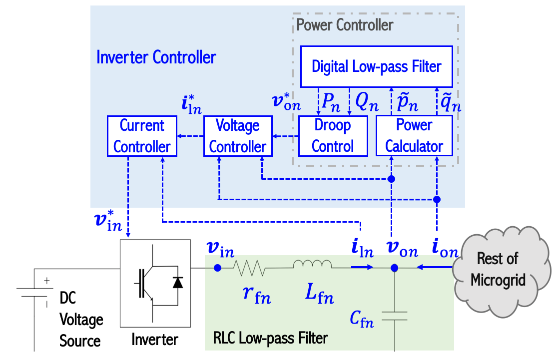
Figure 1: Cyber and physical architecture of IBR $n$.

II-A1 RLC filter

The inverter connects to the rest of the microgrid via an RLC filter whose dynamics are [20]

$$L_{\text{f}n}\dot{i}_{\text{ld}n} =-r_{\text{f}n}i_{\text{ld}n}+L_{\text{f}n}\omega_{0}i_{\text{lq}n}+v_{\text{id}n}-v_{\text{od}n}$$ (1a)

$$L_{\text{f}n}\dot{i}_{\text{lq}n} =-r_{\text{f}n}i_{\text{lq}n}-L_{\text{f}n}\omega_{0}i_{\text{ld}n}+v_{\text{iq}n}-v_{\text{oq}n}$$ (1b)

$$C_{\text{f}n}\dot{v}_{\text{od}n} =C_{\text{f}n}\omega_{0}v_{\text{oq}n}+i_{\text{ld}n}+i_{\text{od}n}$$ (1c)

$$C_{\text{f}n}\dot{v}_{\text{oq}n} =-C_{\text{f}n}\omega_{0}v_{\text{od}n}+i_{\text{lq}n}+i_{\text{oq}n}$$ (1d)

where $i_{\text{ld}n}$ and $i_{\text{od}n}$ ($i_{\text{lq}n}$ and $i_{\text{oq}n}$) are the direct (quadrature) component of the current $\mathbf{i}_{\text{l}n}$ and $\mathbf{i}_{\text{o}n}$ annotated in Figure 1; $v_{\text{id}n}$ and $v_{\text{od}n}$ ($v_{\text{iq}n}$ and $v_{\text{oq}n}$) are the direct (quadrature) components of the voltage $\mathbf{v}_{\text{i}n}$ and $\mathbf{v}_{\text{o}n}$; resistance $r_{\text{f}n}$, inductance $L_{\text{f}n}$, and capacitance $C_{\text{f}n}$ of the RLC circuit are labeled in Figure 1; and $\omega_{0}$ is the nominal frequency (i.e., 377 or 314 rad/s). Note that the reference positive direction of $\mathbf{i}_{\text{o}n}$ is pointing into the IBR.

II-A2 Power controller

A power controller contains a power calculator, a power filter, and a droop controller. The power calculator computes the instantaneous real power $\tilde{p}_{n}$ and reactive power $\tilde{q}_{n}$ injecting into the rest of the microgrid, based on IBR $n$’s terminal voltages ($v_{\text{od}n}$ and $v_{\text{oq}n}$) and current ($i_{\text{od}n}$ and $i_{\text{oq}n}$) in the direct-quadrature (d-q) reference frame of IBR $n$. With the positive reference directions assigned to $\mathbf{v}_{\text{o}n}$ and $\mathbf{i}_{\text{o}n}$ in Figure 1, $\tilde{p}_{n}$ and $\tilde{q}_{n}$ are computed by [20]

$$\tilde{p}_{n}=-(v_{\text{od}n}i_{\text{od}n}+v_{\text{oq}n}i_{\text{oq}n})$$ (2a)

$$\tilde{q}_{n}=-(v_{\text{oq}n}i_{\text{od}n}-v_{\text{od}n}i_{\text{oq}n}).$$ (2b)

The instantaneous real and reactive power feed the power filter, i.e., a digital low-pass filter, whose dynamics is described by

$$\dot{P}_{n} =-\omega_{\text{c}n}P_{n}+\omega_{\text{c}n}\tilde{p}_{n}$$ (3a)

$$\dot{Q}_{n} =-\omega_{\text{c}n}Q_{n}+\omega_{\text{c}n}\tilde{q}_{n}$$ (3b)

where $\omega_{\text{c}n}$ is the cut-off frequency; and $P_{n}$ and $Q_{n}$ are the real and reactive power filtered by the power filter. The droop controller takes $P_{n}$ and $Q_{n}$ as inputs and it specifies frequency $\omega_{n}$, phase angle $\delta_{n}$ and voltage setpoints $v_{\text{od}n}^{*}$ and $v_{\text{oq}n}^{*}$ via

$$\dot{\delta}_{n}=\omega_{n}-\omega_{0},\quad\omega_{n}=\omega_{\text{s}n}-\alpha_{n}P_{n}$$ (4a)

$$v_{\text{od}n}^{*}=V_{\text{0}n}-\beta_{n}Q_{n},\quad v_{\text{oq}n}^{*}=0$$ (4b)

where $\omega_{\text{s}n}$ is set by a secondary controller; $V_{\text{0}n}$ is a voltage setpoint; and $\alpha_{n}$ and $\beta_{n}$ are droop control parameters.

II-A3 Voltage and current controllers

The dynamics of the voltage and current controllers is governed by

$$\dot{\phi}_{\text{d}n}=-v_{\text{od}n}+v_{\text{od}n}^{*},\quad\dot{\phi}_{\text{q}n}=-v_{\text{oq}n}+v_{\text{oq}n}^{*},$$ (5a)

$$\dot{\gamma}_{\text{d}n}=-i_{\text{ld}n}+i_{\text{ld}n}^{*},\quad\dot{\gamma}_{\text{q}n}=-i_{\text{lq}n}+i_{\text{lq}n}^{*},$$ (5b)

$$i_{\text{ld}n}^{*}=K_{\text{pv}n}(v_{\text{od}n}^{*}-v_{\text{od}n})-F_{n}i_{\text{od}n}-\omega_{\text{0}}C_{\text{f}n}v_{\text{oq}n}+K_{\text{iv}n}\phi_{\text{d}n}$$ (5c)

$$i_{\text{lq}n}^{*}=K_{\text{pv}n}(v_{\text{oq}n}^{*}-v_{\text{oq}n})-F_{n}i_{\text{oq}n}+\omega_{\text{0}}C_{\text{f}n}v_{\text{od}n}+K_{\text{iv}n}\phi_{\text{q}n}$$ (5d)

$$v_{\text{id}n}^{*}=K_{\text{pc}n}(i_{\text{ld}n}^{*}-i_{\text{ld}n})-\omega_{\text{0}}L_{\text{f}n}i_{\text{lq}n}+K_{\text{ic}n}\gamma_{\text{d}n}$$ (5e)

$$v_{\text{iq}n}^{*}=K_{\text{pc}n}(i_{\text{lq}n}^{*}-i_{\text{lq}n})+\omega_{\text{0}}L_{\text{f}n}i_{\text{ld}n}+K_{\text{ic}n}\gamma_{\text{q}n}$$ (5f)

where ${\phi}_{\text{d}n}$ and ${\phi}_{\text{q}n}$ (${\gamma}_{\text{d}n}$ and ${\gamma}_{\text{q}n}$) are state variables for the voltage (current) controller; $i_{\text{ld}n}^{*}$ and $i_{\text{lq}n}^{*}$ are setpoints of the current controller provided by the voltage controller; and $K_{\text{pv}n}$, $F_{n}$, $K_{\text{iv}n}$, $K_{\text{pc}n}$, and $K_{\text{ic}n}$ are control parameters.

II-A4 Time scale separation

The state variables of dynamics (1), (3), (4), and (5) include $\delta_{n}$, $P_{n}$, $Q_{n}$, $\phi_{\text{d}n}$, $\phi_{\text{q}n}$, $\gamma_{\text{d}n}$, $\gamma_{\text{q}n}$, $i_{\text{ld}n}$, $i_{\text{lq}n}$, $v_{\text{od}n}$, and $v_{\text{oq}n}$. Define $\mathcal{S}_{n}^{\text{s}}=\{\delta_{n},P_{n},Q_{n}\}$ and $\mathcal{S}_{n}^{\text{f}}=\{\phi_{\text{d}n},\phi_{\text{q}n},\gamma_{\text{d}n},\gamma_{\text{q}n},i_{\text{ld}n},i_{\text{lq}n},v_{\text{od}n},v_{\text{oq}n}\}$. Next we show that the states in $\mathcal{S}_{n}^{\text{f}}$ can be stabilized much faster than those in $\mathcal{S}_{n}^{\text{s}}$ via simulating a grid-connected IBR with a representative parameter setting [20]. The simulation details are reported in Appendix A. In the simulation, the load changes at time $t=0.5$s, Figure 2 visualizes state variables $P_{1}$ and $\phi_{\text{d}1}$. It can be observed that it takes more than $0.15$s to stabilize $P_{1}$, while $\phi_{\text{d}1}$ is stabilized around $0.006$s after the disturbance occurs. Figure 3 presents the stabilization time of key variables of the IBR. Figure 3 suggests that $\omega_{1}$, $P_{1}$, and $Q_{1}$ are stabilized much slower than the states in $\mathcal{S}_{n}^{\text{f}}$. A similar observation is also reported in [21].

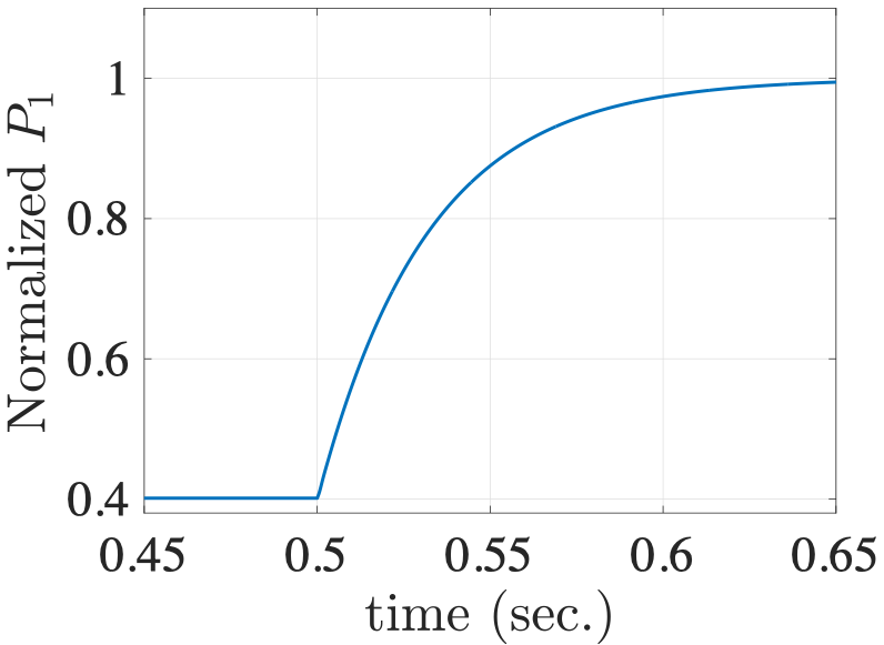
(a)

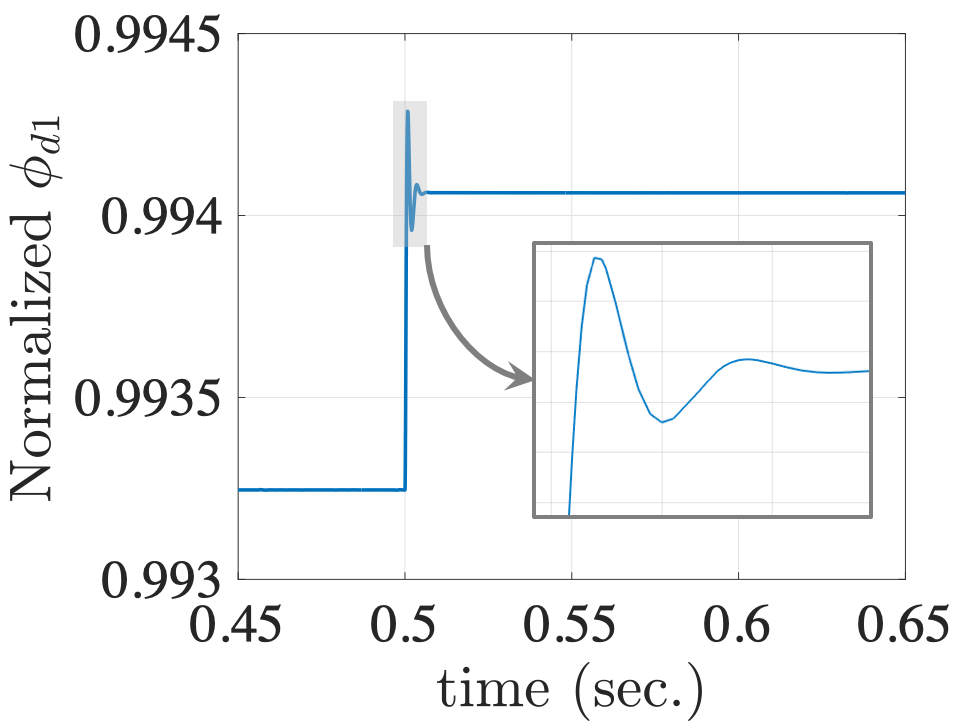
(b)

Figure 2: Time-domain evolution of normalized $P_{1}$ and $\phi_{\text{d}1}$.

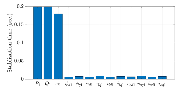
Figure 3: Stabilization time of key variables

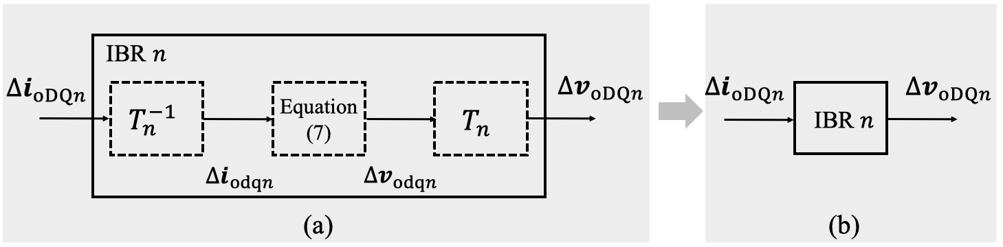
Figure 4: (a) Reference frame transformation; and (b) an input-output perspective of IBR dynamics

A very large body of literature (see [4] and the references therein) studies the slow dynamics defined by the states in $\mathcal{S}_{n}^{\text{s}}$ by assuming that the fast states in $\mathcal{S}_{n}^{\text{f}}$ are stabilized fast. This paper examines the interaction among the fast states in $\mathcal{S}_{n}^{\text{f}}$ by assuming the states in $\mathcal{S}_{n}^{\text{s}}$ as constants. With such an assumption, the IBR dynamics can be described by:

$$\dot{\mathbf{x}}_{n}=A_{n}\mathbf{x}_{n}+B_{n}\mathbf{i}_{\text{odq}n}+B_{n}^{\prime}v^{*}_{\text{od}n}$$ (6a)

$$\mathbf{v}_{\text{odq}n}=C_{n}\mathbf{x}_{n}$$ (6b)

where $\mathbf{x}_{n}=[\phi_{\text{d}n},\phi_{\text{q}n},\gamma_{\text{d}n},\gamma_{\text{q}n},i_{\text{ld}n},i_{\text{lq}n},v_{\text{od}n},v_{\text{oq}n}]^{\top}$; $\mathbf{i}_{\text{odq}n}=[i_{\text{od}n},i_{\text{oq}n}]^{\top}$; $\mathbf{v}_{\text{odq}n}=[v_{\text{od}n},v_{\text{oq}n}]^{\top}$; and matrices $A_{n}$, $B_{n}$, $B_{n}^{\prime}$ and $C_{n}$ are derived from (1) and (5). Since the dynamics (6) is linear, the following equations also hold:

$$\Delta\dot{\mathbf{x}}_{n}=A_{n}\Delta\mathbf{x}_{n}+B_{n}\Delta\mathbf{i}_{\text{odq}n}$$ (7a)

$$\Delta\mathbf{v}_{\text{odq}n}=C_{n}\Delta\mathbf{x}_{n}$$ (7b)

where the “$\Delta$” variables are the deviations from their steady states. The input-output relationship of the dynamics of IBR $n$ is shown in the central block of Figure 4-(a). The input $\Delta\mathbf{i}_{\text{odq}n}$ and output $\Delta\mathbf{v}_{\text{odq}n}$ are represented in the direct-quadrature (d-q) reference frame of the $n$-th IBR, and they interact with the rest of the microgrid in a common reference frame (i.e., D-Q frame). Next, we present the reference frame transformation that converts variables in the d-q frame to the D-Q frame.

II-A5 Reference frame transformation

In Figure 4-(a), the output $\Delta\mathbf{v}_{\text{oDQ}n}:=[\Delta v_{\text{oD}n},\Delta v_{\text{oQ}n}]^{\top}$ is obtained by $\Delta\mathbf{v}_{\text{oDQ}n}=T_{n}\Delta\mathbf{v}_{\text{odq}n}$ where

$$T_{n}=\begin{bmatrix}\cos{\delta_{n}}&-\sin{\delta_{n}}\\ \sin{\delta_{n}}&\cos{\delta_{n}}\end{bmatrix}.$$ (8)

Note that $\delta_{n}$ is assumed to be a constant, since it changes much slower than the states $\mathbf{x}_{n}$ in the time scale of interest. Similarly, the relationship between $\Delta\mathbf{i}_{\text{oDQ}n}:=[\Delta i_{\text{oD}n},\Delta i_{\text{oQ}n}]^{\top}$ and $\Delta\mathbf{i}_{\text{odq}n}$ are described by $\Delta\mathbf{i}_{\text{odq}n}=T_{n}^{-1}\Delta\mathbf{i}_{\text{oDQ}n}$. With the above definitions, IBR $n$ can be viewed as a dynamic system that is driven by $\Delta\mathbf{i}_{\text{oDQ}n}$ while outputting $\Delta\mathbf{v}_{\text{oDQ}n}$, as shown in Figure 4-(b).

II-B Dynamics of Microgrid Network

Assume that the microgrid with $N$ IBRs is three-phase balanced and hosts constant-impedance load. By the Kron reduction technique, the microgrid network can be reduced to a network with $N+1$ node and $M$ branches. One of the $N+1$ node is the neutral/reference point of the microgrid. Let set $\mathcal{N}:=\{0,1,2,\ldots,N\}$ collect the nodal indices of the Kron-reduced network where “$0$” denotes the nodal index for the neutral point. Let set $\mathcal{M}:=\{1,2,\ldots,M\}$ collect branch indices of the reduced network. Another way to represent branch $m$ is to use a pair $(i,j)_{m}$ where $i,j\in\mathcal{N}$ correspond to the two nodes of the two terminals of branch $m$. Suppose that $i<j$, we define the positive direction assigned to branch $m$ is from node $i$ to $j$.

The $M$ branches in the Kron-reduced network can be divided into two categories. Let $\mathcal{E}_{1}$ collect the branches connecting to the neutral point via an IBR, while set $\mathcal{E}_{2}$ collects the rest of the branches. The dynamics of branches in $\mathcal{E}_{1}$ are governed by equations presented in Section II-A, whereas the dynamic behaviors of the branches in $\mathcal{E}_{2}$ are modeled by RL circuits with resistor $r_{\text{b}m}$ and inductance $L_{\text{b}m}$:

$$L_{\text{b}m}\dot{i}_{\text{bD}m}=-r_{\text{b}m}i_{\text{bD}m}+\omega_{0}L_{\text{b}m}i_{\text{bQ}m}+v_{{\text{bD}}m}$$ (9a)

$$L_{\text{b}m}\dot{i}_{\text{bQ}m}=-r_{\text{b}m}i_{\text{bQ}j}-\omega_{0}L_{\text{b}m}i_{\text{bD}m}+v_{{\text{bQ}}m}$$ (9b)

where $m\in\mathcal{E}_{2}$; the subscript “b” reminds readers that the corresponding variables are used for describe branches without IBRs; the subscripts “D” and “Q” suggest the corresponding variables are in the common reference frame (the D-Q frame); $v_{{\text{bD}}m}$ and $v_{{\text{bQ}}m}$ are the bus voltage differences of branch $(i,j)_{m}$ in the D- and Q- axis, i.e., $v_{{\text{bD}}m}=v_{\text{D}i}-v_{\text{D}j}$ and $v_{{\text{bQ}}m}=v_{\text{Q}i}-v_{\text{Q}j}$.

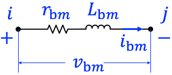
Figure 5: Branch $(i,j)_{m}$ in $\mathcal{E}_{2}$

To characterize the relationship between branch currents $i_{\text{b}m}$ for $m\in\mathcal{M}$, we introduce a reduced incidence matrix $C^{\prime}\in\mathbb{R}^{N\times M}$ whose entries are $c^{\prime}_{n,m}$ with $n\in\mathcal{N}\backslash\{0\}$ and $m\in\mathcal{M}$. Each entry $c^{\prime}_{n,m}$ in matrix $C^{\prime}$ is defined as follows: $c^{\prime}_{n,m}=1$ if branch $m$ is incident at node $n$, and the reference direction of branch $m$ is away from node $n$; $c^{\prime}_{n,m}=-1$ if branch $m$ is incident at node $n$, and the reference direction of branch $m$ is toward to node $n$; and $c^{\prime}_{n,m}=0$ if branch $m$ is not incident at node $n$.

With the reference direction defined before, one can assign indices of nodes and branches such that the reduced incidence matrix $C^{\prime}$ has the following structure [22]

$$C^{\prime}=\begin{bmatrix}C_{0}&-I_{N}\end{bmatrix}$$ (10)

where $C_{0}$ is the first $M-N$ columns of matrix $C^{\prime}$; and $I_{N}$ is a $N$-dimension identity matrix.

Next, we present the compact form of Kirchhoff’s Current Law (KCL), with the incident matrix $C^{\prime}$. Let $M^{\prime}$ be $M-N$. The KCL of the microgrid network in terms of direct/quadrature current leads to

$$C^{\prime}\mathbf{i}_{\text{D}}=\mathbf{0};\quad C^{\prime}\mathbf{i}_{\text{Q}}=\mathbf{0}$$ (11)

where $\mathbf{i}_{\text{D}}=[\mathbf{i}_{\text{bD}}^{\top},\mathbf{i}_{\text{sD}}^{\top}]^{\top}$ with $\mathbf{i}_{\text{bD}}=[i_{\text{bD}1},\ldots,i_{\text{bD}M^{\prime}}]^{\top}$, $\mathbf{i}_{\text{sD}}=[i_{\text{sD}1},\ldots,i_{\text{sD}N}]^{\top}$; and $\mathbf{i}_{\text{Q}}=[\mathbf{i}_{\text{bQ}}^{\top},\mathbf{i}_{\text{sQ}}^{\top}]^{\top}$ with $\mathbf{i}_{\text{bQ}}=[i_{\text{bQ}1},\ldots,i_{\text{bQ}N}]^{\top}$, $\mathbf{i}_{\text{sQ}}=[i_{\text{sQ}1},\ldots,i_{\text{sQ}N}]^{\top}$. Plugging (10) into (11) leads to

$$\mathbf{i}_{\text{sD}}=C_{0}\mathbf{i}_{\text{bD}};\quad\mathbf{i}_{\text{sQ}}=C_{0}\mathbf{i}_{\text{bQ}}.$$ (12)

Moreover, the relationship between the voltages across branches and the nodal voltages can be described by

$$\mathbf{v}_{\text{D}}=C^{\prime\top}\mathbf{v}_{\text{oD}};\quad\mathbf{v}_{\text{Q}}=C^{\prime\top}\mathbf{v}_{\text{oQ}}$$ (13)

In (13), $\mathbf{v}_{\text{D}}=[\mathbf{v}_{\text{bD}}^{\top},\mathbf{v}_{\text{oD}}^{\top}]^{\top}$ and $\mathbf{v}_{\text{Q}}=[\mathbf{v}_{\text{bQ}}^{\top},\mathbf{v}_{\text{oQ}}^{\top}]^{\top}$, where the voltages across branches $\mathbf{v}_{\text{bD}}=[v_{{\text{bD}}1},\ldots,v_{{\text{bD}}M^{\prime}}]^{\top}$; $\mathbf{v}_{\text{bQ}}=[v_{{\text{bQ}}1},\ldots,v_{{\text{bQ}}M^{\prime}}]^{\top}$; and nodal voltages $\mathbf{v}_{\text{oD}}=[v_{\text{oD}1},\ldots,v_{\text{oD}M^{\prime}}]^{\top}$, and $\mathbf{v}_{\text{oQ}}=[v_{\text{oQ}1},\ldots,v_{\text{oQ}M^{\prime}}]^{\top}$ where $v_{\text{oD}m}$ and $v_{\text{oQ}m}$ are obtained by casting $v_{\text{od}m}$ and $v_{\text{oq}m}$ to the D-Q frame by (8).

Plugging (10) into (13) leads to [22]

$$\mathbf{v}_{\text{bD}}=C_{0}^{\top}\mathbf{v}_{\text{oD}};\quad\mathbf{v}_{\text{bQ}}=C_{0}^{\top}\mathbf{v}_{\text{oQ}}$$ (14)

Define the following vectors:

$$\mathbf{i}_{\text{sDQ}}=\begin{bmatrix}\mathbf{i}_{\text{sD}}\\ \mathbf{i}_{\text{sQ}}\end{bmatrix};\mathbf{i}_{\text{bDQ}}=\begin{bmatrix}\mathbf{i}_{\text{bD}}\\ \mathbf{i}_{\text{bQ}}\end{bmatrix};\mathbf{v}_{\text{oDQ}}=\begin{bmatrix}\mathbf{v}_{\text{oD}}\\ \mathbf{v}_{\text{oQ}}\end{bmatrix}.$$ (15)

The branch dynamics (9) can be organized into

$$L\dot{\mathbf{i}}_{\text{bDQ}}=-R\mathbf{i}_{\text{bDQ}}+W\mathbf{i}_{\text{bDQ}}+C^{\top}\mathbf{v}_{\text{oDQ}}$$ (16a)

$$\mathbf{i}_{\text{sDQ}}=C\mathbf{i}_{\text{bDQ}}$$ (16b)

where $L=\text{diag}(L_{1},\ldots,L_{M^{\prime}},L_{1},\ldots,L_{M^{\prime}})$; $R=\text{diag}(r_{1},\ldots,r_{M^{\prime}},r_{1},\ldots,r_{M^{\prime}})$; $C=\begin{bmatrix}C_{0}&C_{0}\end{bmatrix}$; and

$$W=\begin{bmatrix}0_{M^{\prime}\times M^{\prime}}&\omega_{0}I_{M^{\prime}}\\ -\omega_{0}I_{M^{\prime}}&0_{{M^{\prime}}\times{M^{\prime}}}\end{bmatrix}.$$

Since (17) is linear, the following equations also hold:

$$L\Delta\dot{\mathbf{i}}_{\text{bDQ}}=-R\Delta\mathbf{i}_{\text{bDQ}}+W\Delta\mathbf{i}_{\text{bDQ}}+C^{\top}\Delta\mathbf{v}_{\text{oDQ}}$$ (17a)

$$\Delta\mathbf{i}_{\text{sDQ}}=C\Delta\mathbf{i}_{\text{bDQ}}$$ (17b)

where the “$\Delta$” variables are the deviations of the original variables from their steady states.

II-C A Feedback Perspective of Microgrid Dynamics

The interaction between the IBRs and the microgrid network can be interpreted from a feedback perspective shown in Figure 6. The IBR dynamics $\mathcal{F}_{n}$ ($n$= 1, 2, …, N) constitute the feed-forward loop $\mathcal{F}$, whereas the feedback loop $\mathcal{B}$ results from the network dynamics (17). The input of $\mathcal{F}$ is $\Delta\mathbf{i}_{\text{oDQ}}$ defined by $\Delta\mathbf{i}_{\text{oDQ}}=-\Delta\mathbf{i}_{\text{sDQ}}$ where the negative sigh results from the reference directions of $i_{\text{o}n}$ and $i_{\text{s}n}$ defined before: recall that the positive reference direction of $i_{\text{o}n}$ points into the IBR $n$, while the positive reference direction of $i_{\text{s}n}$ points into the network. The output of $\mathcal{F}$ is $\Delta\mathbf{v}_{\text{oDQ}}$ which drives the network dynamics (17).

With Figure 6, the dynamics of the microgrid with $N$ IBRs can be interpreted as follows. At time step $k$, current $\Delta\mathbf{i}_{\text{oDQ}n}[k]$ for $n=1,2,\ldots,N$ drives the dynamics of system $\mathcal{F}$ which updates the internal state variables $\Delta\mathbf{x}_{n}[k+1]$ and outputs voltage $\Delta v_{\text{oDQ}n}[k]$. The voltages $\Delta\mathbf{v}_{\text{oDQ}n}[k]$ further drive the dynamics of the microgrid network to update the internal state variables of the network and produces $\Delta\mathbf{i}_{\text{sDQ}}[k+1]$. The updated currents $\Delta\mathbf{i}_{\text{sDQ}}[k+1]$ drives the dynamics of the IBRs, and the process described above repeats. Such a feedback perspective lends itself to introducing the transient stability protocol based on the passivity theory.

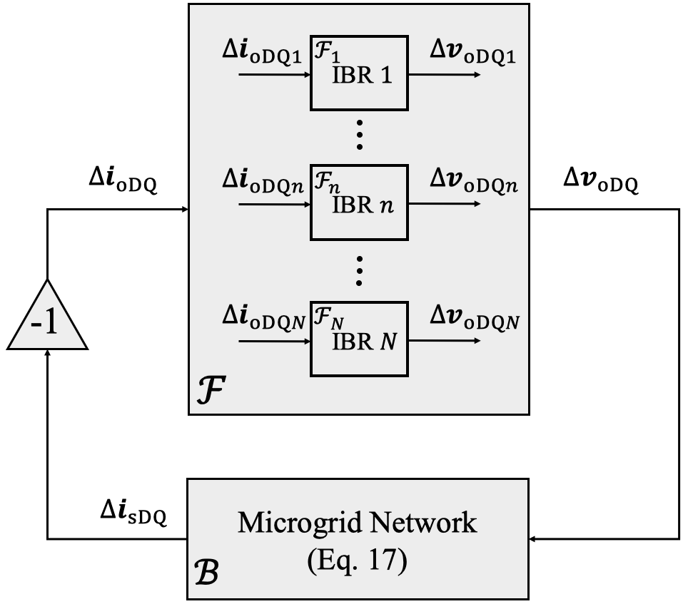
Figure 6: A feedback perspective of microgrid dynamics

III Decentralized Stability Protocol

This section aims to answer the question of what condition each IBR should satisfy such that they can establish a stable microgrid. We term the condition the decentralized stability protocol. This section first introduces some definitions in the control theory. Then we present a lemma that provides guidance to design the protocol. Finally, the the protocol is formally described and justified.

III-A Stability of Interconnected Systems

The closed-loop dynamics of Figure 6 can be described by

$$\dot{\mathbf{x}}=\mathbf{f}(\mathbf{x})$$ (18)

where vector $\mathbf{x}$ collects the IBR states in $\Delta\mathbf{x}_{n}$ for $n=1,\ldots,N$, and the network states in $\Delta\mathbf{i}_{\text{bDQ}}$; and function $\mathbf{f}(\cdot)$ defines the evolution of $\mathbf{x}$ in terms of time. Recall that the equilibrium point of (18) is the origin $\mathbf{o}$. The asymptotic stability of $\mathbf{o}$ is rigorously described by the following definition:

Definition 1.

(Asymptotic stability [23]) The equilibrium point $\mathbf{o}$ of the system (18) is asymptotically stable, if

$$\forall\epsilon>0,\exists\rho>0,\norm{\mathbf{x}(0)}<\rho\implies\norm{\mathbf{x}(t)}<\epsilon,\forall t,$$

and if for some $\rho>0$,

$$\norm{\mathbf{x}(0)}<\rho\implies\lim_{t\rightarrow\infty}\mathbf{x}(t)=\mathbf{o}.$$

For a system $\mathcal{H}$ with input $\mathbf{u}\in\mathbb{R}^{d}$ and output $\mathbf{y}\in\mathbb{R}^{d}$, the next two definitions examine the input-output properties of $\mathcal{H}$:

Definition 2.

(OFP [24]) The system $\mathcal{H}:\mathbf{u}\rightarrow\mathbf{y}$ is output feedback passive (OFP), if for all square integrable $\mathbf{u}(t)$ and some $\sigma>0$,

$$\int_{0}^{t}\mathbf{u}(\tau)^{\top}\mathbf{y}(\tau)d\tau-\sigma\int_{0}^{t}\mathbf{y}(\tau)^{\top}\mathbf{y}(\tau)d\tau\geq 0,$$ (19)

with a zero initial condition. Moreover, $\sigma$ is called the passivity index.

Definition 3.

($\mathcal{L}_{2}$ Gain [24]) The system $\mathcal{H}:\mathbf{u}\rightarrow\mathbf{y}$ has finite $\mathcal{L}_{2}$ gain $\gamma>0$ if for all square integrable $\mathbf{u}$

$$\int_{0}^{t}\mathbf{y}(\tau)^{\top}\mathbf{y}(\tau)d\tau\leq\gamma\int_{0}^{t}\mathbf{u}(\tau)^{\top}\mathbf{u}(\tau)d\tau,$$ (20)

with a zero initial condition.

The link between asymptotic stability and the output feedback passivity is established by the following lemma [24]:

Lemma 1.

(Corollary 1 in [24]) The equilibrium point $\mathbf{o}$ of the closed-loop system in Figure 6 is asymptotically stable, if both subsystems $\mathcal{F}$ and $\mathcal{B}$ are output feedback passive.

Lemma 1 guides one to design a decentralized protocol for each IBR to ensure system-level stability. Subsection III-B examines the OFP property of the feedback loop $\mathcal{B}$ in Figure 6. Subsection III-C introduces the protocol that ensures the OFP property of the feed-forward loop $\mathcal{F}$.

III-B Passivity of Microgrid Networks

The OFP property of the network dynamics (17) in the DQ frame is established by the following theorem:

Theorem 2.

(Network Passivity Index) The microgrid network dynamics (17) is OFP with input $\Delta\mathbf{v}_{\text{oDQ}}$ and output $\Delta\mathbf{i}_{\text{sDQ}}$, if matrix $C^{\top}C$ has at least one positive eigenvalue.

Proof.

By definition,

$$\int_{0}^{t}\Delta\mathbf{i}_{\text{sDQ}}^{\top}\Delta\mathbf{v}_{\text{oDQ}}d\tau=\int_{0}^{t}\Delta\mathbf{i}_{\text{bDQ}}^{\top}C^{\top}\Delta\mathbf{v}_{\text{oDQ}}d\tau$$

$$=\int_{0}^{t}\Delta\mathbf{i}_{\text{bDQ}}^{\top}\left(L\Delta\dot{\mathbf{i}}_{\text{bDQ}}+R\Delta\mathbf{i}_{\text{bDQ}}-W\Delta\mathbf{i}_{\text{bDQ}}\right)d\tau$$

$$=\int_{0}^{t}\left(\Delta\mathbf{i}_{\text{bDQ}}^{\top}L\Delta\dot{\mathbf{i}}_{\text{bDQ}}+\Delta\mathbf{i}_{\text{bDQ}}^{\top}R\Delta\mathbf{i}_{\text{bDQ}}-\Delta\mathbf{i}_{\text{bDQ}}^{\top}W\Delta\mathbf{i}_{\text{bDQ}}\right)d\tau$$

Note that $W=-W^{\top}$ and $\Delta\mathbf{i}_{\text{bDQ}}^{\top}W\Delta\mathbf{i}_{\text{bDQ}}$ is a scalar. Then,

$$\Delta\mathbf{i}_{\text{bDQ}}^{\top}W\Delta\mathbf{i}_{\text{bDQ}} =\left(\Delta\mathbf{i}_{\text{bDQ}}^{\top}W\Delta\mathbf{i}_{\text{bDQ}}\right)^{\top}$$ (21)

$$=-\Delta\mathbf{i}_{\text{bDQ}}^{\top}W\Delta\mathbf{i}_{\text{bDQ}}.$$

Equation (21) leads to $2\Delta\mathbf{i}_{\text{bDQ}}^{\top}W\Delta\mathbf{i}_{\text{bDQ}}=0$, implying

$$\Delta\mathbf{i}_{\text{bDQ}}^{\top}W\Delta\mathbf{i}_{\text{bDQ}}=0.$$ (22)

Based on (21) and (22),

$$\int_{0}^{t}\Delta\mathbf{i}_{\text{sDQ}}^{\top}\Delta\mathbf{v}_{\text{oDQ}}d\tau=V(t)-V_{0}+\int_{0}^{t}\Delta\mathbf{i}_{\text{bDQ}}^{\top}R\Delta\mathbf{i}_{\text{bDQ}}d\tau$$

where $V(t):=0.5\Delta\mathbf{i}_{\text{bDQ}}^{\top}(t)L\Delta\mathbf{i}_{\text{bDQ}}(t)$ and $V_{0}:=0.5\Delta\mathbf{i}_{\text{bDQ}}^{\top}(0)L\Delta\mathbf{i}_{\text{bDQ}}(0)$. As matrices $L\succ 0$,

$$\int_{0}^{t}\Delta\mathbf{i}_{\text{sDQ}}^{\top}\Delta\mathbf{v}_{\text{oDQ}}d\tau\geq-V_{0}+\int_{0}^{t}\Delta\mathbf{i}_{\text{bDQ}}^{\top}R\Delta\mathbf{i}_{\text{bDQ}}d\tau$$ (23)

$$\geq-V_{0}+\lambda_{\text{Rmin}}\int_{0}^{t}\Delta\mathbf{i}_{\text{bDQ}}^{\top}\Delta\mathbf{i}_{\text{bDQ}}d\tau$$

$$\geq-V_{0}+\frac{\lambda_{\text{Rmin}}}{\lambda_{\text{Cmax}}}\int_{0}^{t}\Delta\mathbf{i}_{\text{sDQ}}^{\top}\Delta\mathbf{i}_{\text{sDQ}}d\tau$$

where $\lambda_{\text{Rmin}}$ is the minimal eigenvalue of $R$; $\lambda_{\text{Cmax}}$ is the maximal eigenvalue of $C^{\top}C$; and $\lambda_{\text{Cmax}}>0$ as $C^{\top}C\succeq 0$. The third line of (23) is due to the fact that

$$\Delta\mathbf{i}_{\text{sDQ}}^{\top}\Delta\mathbf{i}_{\text{sDQ}} =\Delta\mathbf{i}_{\text{bDQ}}^{\top}C^{\top}C\Delta\mathbf{i}_{\text{bDQ}}$$ (24)

$$\leq\lambda_{\text{Cmax}}\Delta\mathbf{i}_{\text{bDQ}}^{\top}\Delta\mathbf{i}_{\text{bDQ}.}$$

The inequality (19) is evaluated with a zero initial condition. By setting $\Delta\mathbf{i}_{\text{bDQ}}(0)=0$, it follows that $V_{0}=0$ and dynamics (17) is OFP with passivity index $\lambda_{\text{Rmin}}/\lambda_{\text{Cmax}}$. ∎

Remark: The proof of Theorem 2 reveals that the passivity index of an RL network depends not only on the minimal branch resistance, but also on the branches’ connectivity.

III-C IBR-level Stability Protocol

Theorem 2 suggests that the feedback loop $\mathcal{B}$ in Figure 6 is OFP. According to Lemma 1, the system-level asymptotic stability can be established, if the feed-forward loop $\mathcal{F}$ is OFP. This observation inspires us to design the following IBR-level stability protocol that leads to the microgrid-level stability:

Protocol 1: For $n=1,2,\ldots,N$, the dynamics of IBR $n$ with input $\Delta\mathbf{i}_{\text{odq}n}$ and output $\Delta\mathbf{v}_{\text{odq}n}$ is OFP.

The “P(assive)” in Protocol 1 should not be confused with the “passive element” defined in the circuit theory [25]. In the circuit theory, the passive element is an element that is “not capable of generating energy” [25]. However, whether an OFP component in the sense of Definition 2 is capable of generating energy or not depends on the definition of its inputs and outputs. If an IBR follows Protocol 1, it does not mean that the IBR cannot produce energy that powers its host microgrid, and it essentially means that the IBR cannot produce energy that leads disturbances to be sustained or amplified. Section V shows an example that a IBR follows Protocol 1 but produces energy. Next we show following Protocol 1 leads to asymptotic stability.

Theorem 3.

The equilibrium point of the closed-loop system in Figure 6 is asymptotically stable if Protocol 1 is followed.

Proof.

Protocol 1 requires each IBR to be OFP, i.e., there exist $\sigma_{n}>0$ such that, for $n=1,2,\ldots,N$,

$$\int_{0}^{t}\Delta\mathbf{i}_{\text{odq}n}^{\top}\Delta\mathbf{v}_{\text{odq}n}d\tau-\sigma_{n}\int_{0}^{t}\Delta\mathbf{v}_{\text{odq}n}^{\top}\Delta\mathbf{v}_{\text{odq}n}d\tau\geq 0$$ (25)

According to Figure 4-(a), $\Delta\mathbf{i}_{\text{odq}n}=T_{n}^{-1}\Delta\mathbf{i}_{\text{oDQ}n}$ and $\Delta\mathbf{v}_{\text{odq}n}=T_{n}^{-1}\Delta\mathbf{v}_{\text{oDQ}n}$, then

$$\int_{0}^{t}\Delta\mathbf{i}_{\text{oDQ}n}^{\top}(T_{n}^{-1})^{\top}T_{n}^{-1}\Delta\mathbf{v}_{\text{oDQ}n}d\tau-$$ (26)

$$\sigma_{n}\int_{0}^{t}\Delta\mathbf{v}_{\text{oDQ}n}^{\top}(T_{n}^{-1})^{\top}T_{n}^{-1}\Delta\mathbf{v}_{\text{oDQ}n}d\tau\geq 0$$

Note that $(T_{n}^{-1})^{\top}T_{n}^{-1}=I$. This leads to

$$\int_{0}^{t}\Delta\mathbf{i}_{\text{oDQ}n}^{\top}\Delta\mathbf{v}_{\text{oDQ}n}d\tau-\sigma_{n}\int_{0}^{t}\Delta\mathbf{v}_{\text{oDQ}n}^{\top}\Delta\mathbf{v}_{\text{oDQ}n}d\tau\geq 0$$ (27)

Define $\underline{\sigma}:=\min_{n}\sigma_{n}$. It follows that

$$\int_{0}^{t}\Delta\mathbf{i}_{\text{oDQ}n}^{\top}\Delta\mathbf{v}_{\text{oDQ}n}d\tau-\underline{\sigma}\int_{0}^{t}\Delta\mathbf{v}_{\text{oDQ}n}^{\top}\Delta\mathbf{v}_{\text{oDQ}n}d\tau\geq 0$$ (28)

for $n=1,2,\ldots,N$. By summing up the $N$ inequalities in (28), we have

$$\sum_{n=1}^{N}\int_{0}^{t}\Delta\mathbf{i}_{\text{oDQ}n}^{\top}\Delta\mathbf{v}_{\text{oDQ}n}d\tau-\underline{\sigma}\sum_{n=1}^{N}\int_{0}^{t}\Delta\mathbf{v}_{\text{oDQ}n}^{\top}\Delta\mathbf{v}_{\text{oDQ}n}d\tau\geq 0.$$

Since $N$ is finite, the finite summation and integration operators can be interchanged, i.e.,

$$\int_{0}^{t}\sum_{n=1}^{N}\Delta\mathbf{i}_{\text{oDQ}n}^{\top}\Delta\mathbf{v}_{\text{oDQ}n}d\tau-\underline{\sigma}\int_{0}^{t}\sum_{n=1}^{N}\Delta\mathbf{v}_{\text{oDQ}n}^{\top}\Delta\mathbf{v}_{\text{oDQ}n}d\tau\geq 0.$$

Note that $\sum_{n=1}^{N}\Delta\mathbf{i}_{\text{oDQ}n}^{\top}\Delta\mathbf{v}_{\text{oDQ}n}=\Delta\mathbf{i}_{\text{oDQ}}^{\top}\Delta\mathbf{v}_{\text{oDQ}}$ and $\sum_{n=1}^{N}\Delta\mathbf{v}_{\text{oDQ}n}^{\top}\Delta\mathbf{v}_{\text{oDQ}n}=\Delta\mathbf{v}_{\text{oDQ}}^{\top}\Delta\mathbf{v}_{\text{oDQ}}$. This leads to

$$\int_{0}^{t}\Delta\mathbf{i}_{\text{oDQ}}^{\top}\Delta\mathbf{v}_{\text{oDQ}}d\tau-\underline{\sigma}\int_{0}^{t}\Delta\mathbf{v}_{\text{oDQ}}^{\top}\Delta\mathbf{v}_{\text{oDQ}}d\tau\geq 0.$$

By Definition 2, the subsystem $\mathcal{F}$ in Figure 6 is OFP with passivity index $\underline{\sigma}$. In addition, since subsystem $\mathcal{B}$ is OFP according to Theorem 2, the asymptotic stability of equilibrium of the system in Figure 6 is established by Lemma 1. ∎

As Protocol $1$ is not straight-forward to implement for IBR manufacturers, how do they enforce protocol 1? This is answered in the next section.

IV Non-intrusive Protocol Enforcement

In this section, we first illustrate the basic idea of enforcing Protocol 1. Then we conceptualize the architecture of an interface that enforces Protocol 1 in a non-intrusive way. We also define the information needed to design the interface.

IV-A Basic Idea of Protocol Enforcement

Protocol 1 at IBR $n$ can be enforced by the scheme shown in Figure 7 where $\alpha_{n}$, $\beta_{n}$, and $\kappa_{n}$ are tunable parameters; and $I$ is an identity matrix. The next lemma guides one to tune $\alpha_{n}$, $\beta_{n}$, and $\kappa_{n}$ to follow Protocol 1:

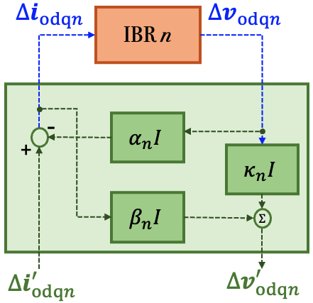
Figure 7: Basic idea of enforcing the Stability Protocol

Lemma 4.

(Theorem 4 in [26]) The closed-loop system in Figure 7 with input $\Delta\mathbf{i}^{\prime}_{\text{odq}n}$ and output $\Delta\mathbf{v}^{\prime}_{\text{odq}n}$ is OFP with $\sigma_{n}=0.5(\frac{1}{\beta_{n}}+\frac{\alpha_{n}}{\kappa_{n}})>0$, if

$$\beta_{n}\geq\kappa_{n}\gamma_{n}>0,\quad\kappa_{n}>\alpha_{n}\beta_{n}>0,$$ (29)

where $\gamma_{n}$ is the $\mathcal{L}_{2}$ gain of the IBR $n$ with input $\Delta\mathbf{i}_{\text{odq}n}$ and output $\Delta\mathbf{v}_{\text{odq}n}$ in Figure 7.

Suppose that an IBR manufacturer provides an $\mathcal{L}_{2}$ gain $\gamma_{n}$, the NMPs can leverage Algorithm 1 to find $\alpha_{n}$, $\beta_{n}$, and $\kappa_{n}$. It is easy to verify that the $\alpha_{n}$, $\beta_{n}$, and $\kappa_{n}$ returned by Algorithm 1 satisfy constraints (29). As a result, the closed-loop system shown in Figure 7 follows Protocol 1. The remaining question is: how does the IBR manufacturer compute $\gamma_{n}$?

Algorithm 1 Non-manufacturer Parties’ Algorithm

1:input: $\gamma_{n}$

2:$\bar{\beta}\leftarrow 0.5$; $\bar{\sigma}\leftarrow 0.5$; $\texttt{flag}\leftarrow 0$

3:while $k_{1}=1,2,\ldots,K$ do

4:     Pick an arbitrary $\sigma_{0}>0$ and $\sigma_{0}\neq\bar{\sigma}$

5:     while $k_{2}=1,2,\ldots,K$ do

6:         Pick an arbitrary $\beta_{0}>0$ and $\beta_{0}\neq\bar{\beta}$

7:         $\kappa_{0}\leftarrow\beta_{0}/(1.05\gamma_{n})$;  $\alpha_{0}\leftarrow 2\sigma_{n}\beta_{0}/\gamma_{n}-1/\gamma_{n}$

8:         if $\kappa_{0}>\alpha_{0}\beta_{0}\wedge\alpha_{0}>0$  then

9:              $\alpha_{n}\leftarrow\alpha_{0}$; $\beta_{n}\leftarrow\beta_{0}$; $\kappa_{n}\leftarrow\kappa_{0}$; $\texttt{flag}\leftarrow 1$

10:              break

11:         else$\quad\bar{\beta}\leftarrow\beta_{0}$

12:         end if

13:     end while

14:     if $\texttt{flag}==1$ then break

15:     else$\quad\bar{\sigma}\leftarrow\sigma_{0}$

16:     end if

17:end while

18:return $\alpha_{n}$, $\beta_{n}$, $\kappa_{n}$

IV-B $\mathcal{L}_{2}$ Gain for IBRs

Algorithm 2 can be leveraged by IBR manufacturers to obtain $\gamma_{n}$, and it is designed based on the following lemma:

Lemma 5.

[23] Assume that the real part of every eigenvalue of matrix $A_{n}$ in (7) is strictly negative. Let $G_{n}(s)=C_{n}(sI-A_{n})^{-1}B_{n}$. Then, the $\mathcal{L}_{2}$ gain of dynamics (7) is $\sup_{\omega\in\mathbb{R}}\norm{G_{n}(\mathbbm{j}\omega)}_{2}$.

In Lemma 5, $\norm{\cdot}_{2}$ is the $\mathcal{L}_{2}$ norm; $\mathbbm{j}=\sqrt{-1}$; and $\sup_{\omega\in\mathbb{R}}\norm{G_{n}(j\omega)}_{2}$ is the $H_{\infty}$ norm of $G_{n}(\mathbbm{j}\omega)$ [23] which can be obtained by standard procedures, e.g., the “hinfnorm” function in MATLAB, given matrices $A_{n}$, $B_{n}$, and $C_{n}$. Lemma 5 requires a stable matrix $A_{n}$. This is not a big assumption, as IBR control designers typically perform small-signal analysis to ensure device-level stability.

Algorithm 2 Manufacturers’ Algorithm

1:input: $A_{n}$, $B_{n}$, and $C_{n}$

2:Obtain $G_{n}(s)$ by $G_{n}(s)=C_{n}(sI-A_{n})^{-1}B_{n}$

3:$\gamma_{n}\leftarrow\texttt{hinfnorm}(G_{n})$

4:return $\gamma_{n}$

IV-C Architecture of Protocol Enforcement Interfaces (PEI)

This subsection conceptualizes an interface that enforce Protocol 1. The physical layer of the interface is shown in Figure 8. The interface comprises a three-phase, controlled volage source, and a three-phase controlled current source. The voltage $\Delta\mathbf{v}_{\text{abc}n}:=[\Delta v_{\text{a}n},\Delta v_{\text{b}n},\Delta v_{\text{c}n}]^{\top}$ of the voltage source and the current $\Delta\mathbf{i}_{\text{abc}n}:=[\Delta i_{\text{a}n},\Delta i_{\text{b}n},\Delta i_{\text{c}n}]^{\top}$ of the current source are determined by the terminal voltage measurement $\mathbf{v}_{\text{abc}n}:=[v_{\text{a}n},v_{\text{b}n},v_{\text{c}n}]^{\top}$ and current measurement $\mathbf{i}_{\text{abc}n}:=[i_{\text{a}n},i_{\text{b}n},i_{\text{c}n}]^{\top}$ of the IBR $n$. This paper focuses on the control law that establishes the link between $\{\mathbf{v}_{\text{abc}n},\mathbf{i}_{\text{abc}n}\}$ and $\{\Delta\mathbf{v}_{\text{abc}n},\Delta\mathbf{i}_{\text{abc}n}\}$; the internal design of the controlled voltage and current sources is out of the scope of this paper.

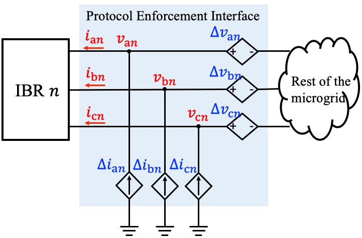
Figure 8: Physical layer of the protocol enforcement interface

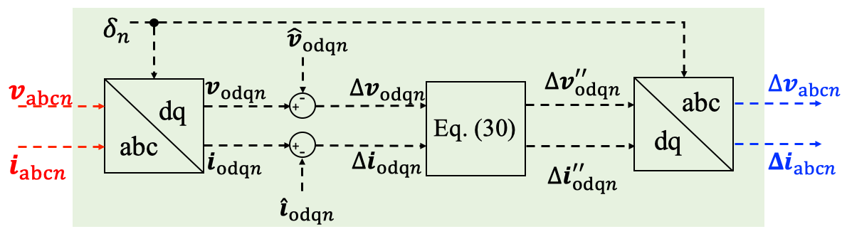
Figure 9: Cyber layer of the protocol enforcement interface.

Figure 9 presents the cyber layer of the interface. In Figure 9, the three-phase variables $\mathbf{v}_{\text{abc}n}$ and $\mathbf{i}_{\text{abc}n}$ are first transformed into the d-q frame by the Park transformation: $[v_{\text{od}},v_{\text{oq}},v_{\text{o0}}]^{\top}=T_{n}^{\prime}[v_{\text{a}},v_{\text{b}},v_{\text{c}}]^{\top}$; and $[i_{\text{od}},i_{\text{oq}},i_{\text{o0}}]^{\top}=T_{n}^{\prime}[i_{\text{a}},i_{\text{b}},i_{\text{c}}]^{\top}$ where [27]

$$T_{n}^{\prime}=\frac{2}{3}\begin{bmatrix}\sin\theta_{n}&\sin(\theta_{n}-\frac{2\pi}{3})&\sin(\theta_{n}+\frac{2\pi}{3})\\ \cos\theta_{n}&\cos(\theta_{n}-\frac{2\pi}{3})&\cos(\theta_{n}+\frac{2\pi}{3})\\ \frac{1}{2}&\frac{1}{2}&\frac{1}{2}\end{bmatrix}.$$

In the above equation, $\theta_{n}=\omega_{n}t+\delta_{n}$, and $\theta_{n}$ can be obtained locally by a phase-locked loop [28]. Second, the deviation vectors $\Delta\mathbf{v}_{\text{odq}n}$ and $\Delta\mathbf{i}_{\text{odq}n}$ are obtained by subtracting the steady-state values $\hat{\mathbf{v}}_{\text{odq}n}$ and $\hat{\mathbf{i}}_{\text{odq}n}$ from $\mathbf{v}_{\text{odq}n}$ and $\mathbf{i}_{\text{odq}n}$. Third, $\Delta\mathbf{v}_{\text{odq}n}^{\prime\prime}$ and $\Delta\mathbf{i}_{\text{odq}n}^{\prime\prime}$ are computed by

$$\Delta\mathbf{v}_{\text{odq}n}^{\prime\prime}=(I-\kappa_{n}I)\Delta\mathbf{v}_{\text{odq}n}-\beta_{n}I\Delta\mathbf{i}_{\text{odq}n}$$ (30a)

$$\Delta\mathbf{i}_{\text{odq}n}^{\prime\prime}=-\alpha_{n}I\Delta\mathbf{v}_{\text{odq}n}.$$ (30b)

Finally, the vectors in the d-q frame $\Delta\mathbf{v}_{\text{odq}n}^{\prime\prime}$ and $\Delta\mathbf{i}_{\text{odq}n}^{\prime\prime}$ are transformed to the three-phase frame.

Equation (30) is justified by transforming Figure 8 in the three-phase frame to the d-q frame. Figure 10 presents the circuit in the d-q frame. According to Figure 7, we have

$$\Delta\mathbf{v}_{\text{odq}n}^{\prime}=\kappa_{n}I\Delta\mathbf{v}_{\text{odq}n}+\beta_{n}I\Delta\mathbf{i}_{\text{odq}n}$$ (31a)

$$\Delta\mathbf{i}_{\text{odq}n}^{\prime}=\alpha_{n}I\Delta\mathbf{v}_{\text{odq}n}+\Delta\mathbf{i}_{\text{odq}n}.$$ (31b)

In Figure 10, based on the Kirchhoff’s circuit laws, we have

$$\Delta\mathbf{v}_{\text{odq}n}^{\prime}=\Delta\mathbf{v}_{\text{odq}n}-\Delta\mathbf{v}_{\text{odq}n}^{\prime\prime}$$ (32a)

$$\Delta\mathbf{i}_{\text{odq}n}^{\prime}=\Delta\mathbf{i}_{\text{odq}n}-\Delta\mathbf{i}_{\text{odq}n}^{\prime\prime}.$$ (32b)

Plugging (32) into (31) leads to (30).

It is worth noting that designing the interface shown in Figures 8 and 9 only requires an IBR manufacturer to provide the $\mathcal{L}_{2}$ gains of their IBRs which can be easily obtained via Algorithm 2 by the manufacturer. The interface design does not need the information of detailed IBR control. While the IBR manufacturer may be reluctant to share such information with the NMPs due to privacy concerns on intellectual properties, revealing the $\mathcal{L}_{2}$ of the IBRs does not lead to such privacy issues, as it is impossible to infer the detailed control design of an IBR merely based on the $\mathcal{L}_{2}$ gains of the IBR.

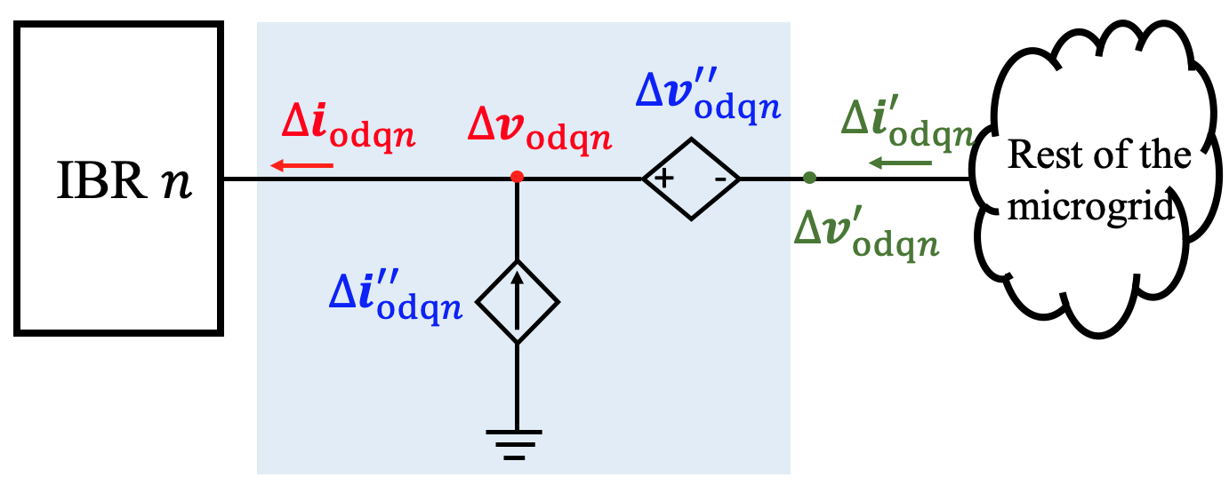
Figure 10: Physical layer of the protocol enforcement interface in the d-q frame

V Case Study

This section tests the effectiveness of the PEIs by simulating the two networked microgrids shown in Figure 11.

V-A Motivating Example

The test system in Figure 11 contains two microgrids. All control parameters of IBR $1$ can be found in [20]. For IBR $2$, $k_{\text{iv}2}=78$, and the rest of parameters are from [20]. The per-phase impedances of Loads $1$ and $2$ are 25$\Omega$ and 20$\Omega$, respectively. Before time $t=0.4$s, Microgrids 1 and 2 are in the islanded mode. At $t=0.4$s, the two small microgrids are networked via the tie line and they enter the hybrid mode. Figures 12 visualizes the three-phase terminal currents at both IBRs, i.e., $\mathbf{i}_{\text{abc}1}$ and $\mathbf{i}_{\text{abc}2}$, from $0.2$s to $1$s. In Figures 12, it can be observed that the magnitudes of $\mathbf{i}_{\text{abc}1}$ and $\mathbf{i}_{\text{abc}2}$ are constant before the two microgrids are networked, i.e., $t<0.4$s. This suggests the two microgrids in the islanded mode are stable. However, after the two microgrids are networked, i.e., $t>0.4$s, the magnitudes of $\mathbf{i}_{\text{abc}1}$ and $\mathbf{i}_{\text{abc}2}$ keep oscillating. Figure 13 examines the three-phase currents $\mathbf{i}_{\text{abc}1}$ and $\mathbf{i}_{\text{abc}2}$ in the d-q frame: before $t=0.4$s, both $\mathbf{i}_{\text{odq}1}$ and $\mathbf{i}_{\text{odq}2}$ can be stabilized at their nominal values. However, after the switch is closed at $t=0.4$s, both $\mathbf{i}_{\text{odq}1}$ and $\mathbf{i}_{\text{odq}2}$ keep oscillating with increasing amplitudes, suggesting that the two networked microgrids become unstable.

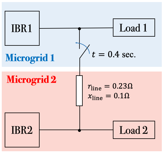
Figure 11: Two networked microgrids

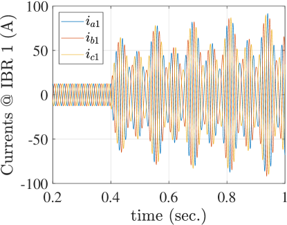
(a)

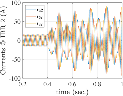
(b)

Figure 12: Time-domain evolution of (a) $\mathbf{i}_{\text{abc}1}$ and (b) $\mathbf{i}_{\text{abc}2}$.

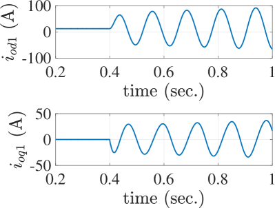
(a)

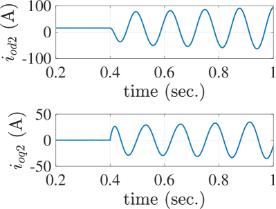
(b)

Figure 13: (a) Time-domain evolution of (a) $\{i_{\text{od}1},i_{\text{oq}1}\}$ and (b) $\{i_{\text{od}2},i_{\text{oq}2}\}$

V-B Performance of Protocol Enforcement Interfaces

V-B1 System responses with protocol enforcement interface

With the same setting of Section V-A, each IBR connects a PEI shown in Figure 8. The manufacturer of each IBR can use Algorithm 2 to obtain the $\mathcal{L}_{2}$ gain $\gamma_{n}$ of the IBR. With the $\mathcal{L}_{2}$ gain $\gamma_{n}$, NMPs can find the parameters of each PEI, i.e., $\alpha_{n}$, $\beta_{n}$, and $\kappa_{n}$, via Algorithm 1. It is worth noting that the manufacturer does not need to share the detailed model of their IBRs with the NMPs to enable them to design the PEI. The $\mathcal{L}_{2}$ gain $\gamma_{n}$ obtained from Algorithm 2 and the interface parameters $\alpha_{n}$, $\beta_{n}$, and $\kappa_{n}$ computed by Algorithm 1 are listed in Table I. It can be easily verified that condition (29) is satisfied.

Figures 14 and 15 show the performance of PEIs. It can be observed that after the two microgrids are networked at $t=0.4$ s, the three-phase current magnitudes are constant after some transients. Figure 16 visualizes the d-q components $\mathbf{i}_{\text{odq}1}$ and $\mathbf{i}_{\text{odq}2}$: the PEIs can stabilize the currents at constant values after the two IBRs are networked, while both $\mathbf{i}_{\text{odq}1}$ and $\mathbf{i}_{\text{odq}2}$ would keep oscillating with increasing amplitudes if no PEI is installed (shown in Figure 13).

TABLE I: Parameters of Protocol Enforcement Interface

$n$	$\gamma_{n}$	$\sigma_{n}$	$\alpha_{n}$	$\beta_{n}$	$\kappa_{n}$
$1$	$6.45$	$3$	$0.0031$	$0.17$	$0.0251$
$2$	$4.23$	$3.5$	$0.0118$	$0.15$	$0.0338$

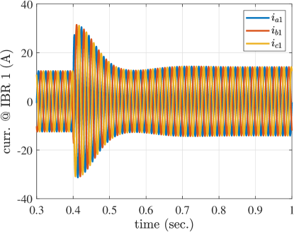
(a)

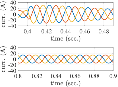
(b)

Figure 14: (a) Time-domain evolution of instantaneous currents (curr.) $\textbf{i}_{\text{abc}1}$ at IBR 1 with the passivisation interface; (b) Zoomed-in version of $\textbf{i}_{\text{abc}1}$ during the transients (the upper panel) and the steady state (the lower panel).

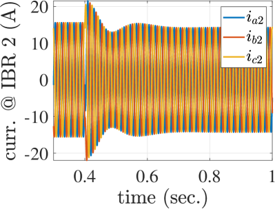
(a)

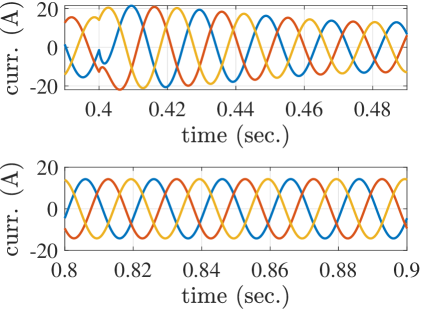
(b)

Figure 15: (a) Time-domain evolution of instantaneous currents (curr.) $\textbf{i}_{\text{abc}2}$ at IBR 2 with the passivisation interface; (b) Zoomed-in version of $\textbf{i}_{\text{abc}2}$ during the transients (the upper panel) and the steady state (the lower panel).

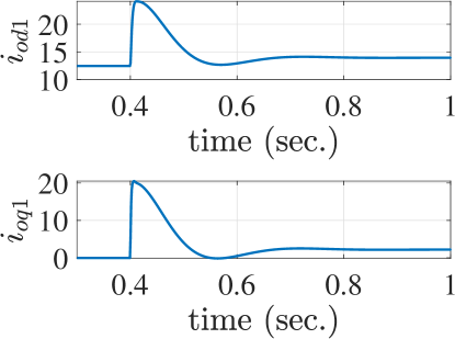
(a)

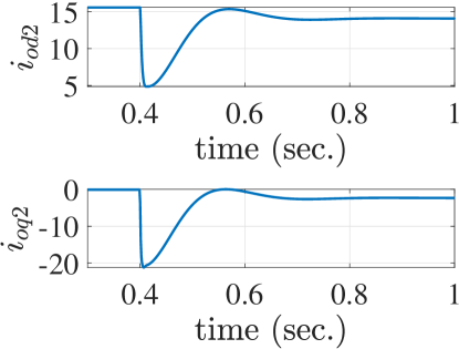
(b)

Figure 16: Time-domain evolution of (a) $\textbf{i}_{\text{odq}1}$ and (b) $\textbf{i}_{\text{odq}2}$ with the PEIs.

V-B2 Impact of PEIs

Do the PEIs consume significant amount of energy to stabilize the microgrids? We answer this question by comparing the energy consumed by the interfaces with the energy produced by the IBRs. For $n=1,2$, denote by $P_{n}$, $P_{\text{c}n}$, and $P_{\text{v}n}$ the real power produced by IBR $n$, the real power consumed by the three-phase, shunt current source in the PEI at IBR $n$, and the real power consumed by the three-phase, series voltage source in the PEI at IBR $n$, respectively. Denote by $E_{n}$, $E_{\text{c}n}$, and $E_{\text{v}n}$ the energy produced by IBR $n$, the energy consumed by the three-phase current source in the PEI at IBR $n$, and the energy consumed by the three phase voltage source in the PEI at IBR $n$, over a period.

Figure 17 visualize $P_{n}$, $P_{\text{c}n}$, and $P_{\text{v}n}$. In Figure 17-(a), it can be observed that the real power used for stabilizing the microgrids, i.e., $P_{\text{c}1}$ and $P_{\text{v}1}$, is much less than $P_{1}$. By integrating $P_{1}$, $P_{\text{c}1}$, and $P_{\text{v}1}$ over a period, $E_{1}$, $E_{\text{c}1}$, and $E_{\text{v}1}$ over the period, can be computed. Table II presents $E_{1}$, $E_{\text{c}1}$, and $E_{\text{v}1}$ over the transient process (i.e., the process from $0.4$s to $0.7$s) and the steady state (i.e., the process from $0.7$s to $1$s). Let $E_{\text{I}n}=E_{\text{c}1}+E_{\text{v}1}$ for $n=1,2$. It can be seen that the PEI at IBR 1 only takes a very small amount of energy, i.e., $1.66\%$ of total energy produced by IBR 1 during the transients, to stabilize the microgrids. In the steady state, the energy consumed by the PEI is only $0.51\%$ of the total energy produced by the IBR $1$.

Similarly, Figure 17-(b) shows that after the two IBR, the absolute value of real power consumed by the interface at IBR $2$ is much smaller than the real power produced by IBR $2$. The values of $E_{2}$, $E_{\text{c}2}$ and $E_{\text{v}2}$ over the transient process ($0.4$s - $0.7$s) and the steady state ($0.7$s - $1$s) are reported in Table II. It can be seen that the protocol enforcement interface at IBR 2 actually produces energy to stabilize the system, as $E_{\text{c}2}$ and $E_{\text{v}2}$ are negative in Table II. Compared with the energy produced by IBR $2$, the energy produced by IBR $2$ for the stabilization purpose is very small, i.e., $0.91\%$ of $E_{2}$ during the transients and $0.61\%$ of $E_{2}$ during the steady state.

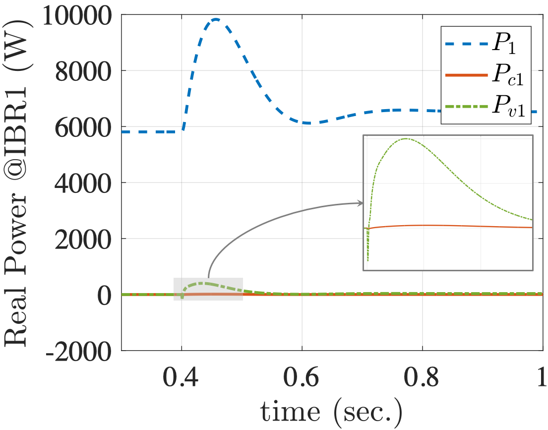
(a)

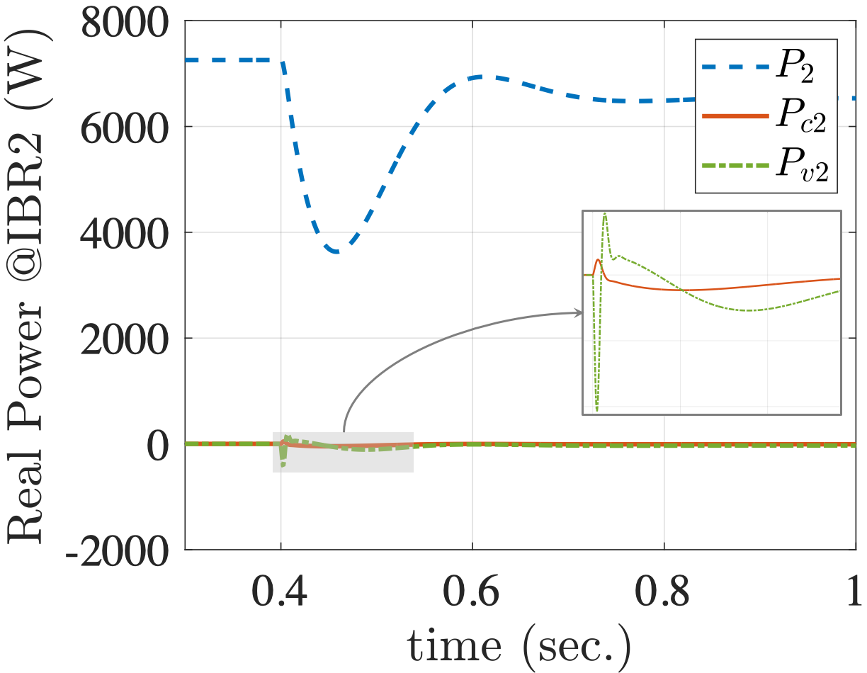
(b)

Figure 17: (a) Time-domain evolution of $P_{1}$, $P_{\text{v}1}$, and $P_{\text{c}1}$ at IBR 1; and (b) time-domain evolution of $P_{2}$, $P_{\text{v}2}$, and $P_{\text{c}2}$

TABLE II: Energy Analysis

Period	$E_{1}$ (J)	$E_{\text{c}1}$ (J)	$E_{\text{v}1}$ (J)	$\absolutevalue{E_{\text{I}1}/E_{1}}$ (%)
$0.4$s - $0.7$s	$2214.4$	$1.36$	$35.54$	$1.67\%$
$0.7$s - $1$s	$1963.4$	$0.6$	$10.57$	$0.57\%$
Period	$E_{2}$ (J)	$E_{\text{c}2}$ (J)	$E_{\text{v}2}$ (J)	$\absolutevalue{E_{\text{I}2}/E_{2}}$ (%)
$0.4$s - $0.7$s	$1737.4$	$-4.94$	$-10.82$	$0.91\%$
$0.7$s - $1$s	$1955.9$	$-2.31$	$-9.66$	$0.61\%$

V-B3 The role of $\sigma_{n}$

Figure 18 visualizes the response of $i_{\text{od}1}$ under the same disturbance in Section V-A with different $\sigma_{1}$. In the simulation, $\sigma_{1}=\sigma_{2}$. It can be observed that all responses are stabilized with $\sigma_{1}$ listed in Figure 18, but larger $\sigma_{1}$ leads to larger overshooting. Table III shows the energy consumed by the PEIs at IBRs $1$ and $2$. Table III and Figure 18 suggest that it is not wise to choose a large $\sigma_{n}$ (e.g., $\sigma_{n}=30$), as a large $\sigma_{n}$ leads to both large overshooting and large energy consumption/generation of the PEIs.

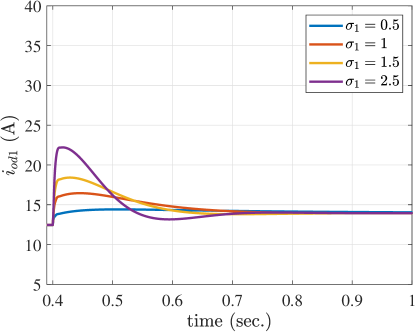
(a)

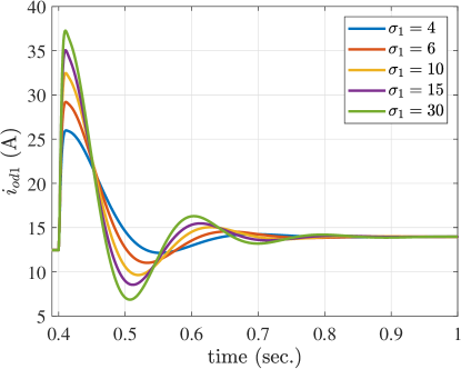
(b)

Figure 18: Response of $i_{\text{od}1}$ with different $\sigma_{1}$

TABLE III: Energy Consumed by Interfaces 1 and 2 with Different $\sigma_{1}$

$\sigma_{1}$	$0.5$	$1$	$1.5$	$2.5$	$4$	$6$	$10$	$15$	30
$E_{\text{I}1}$ (J)	101	78	67	50	46	43	47	43	73
$E_{\text{I}2}$ (J)	-16	-30	-32	-23	-23	-24	-33	-29	-76

VI Conclusion

This paper introduces passivity-based stability protocol for IBRs in AC microgrids. The protocol is enforced by a novel interface at the grid edge in a decentralized, non-intrusive manner. The proposed method is tested by simulating two networked microgrids with benchmark parameters. Simulations show that growing oscillations can occur, when two stable AC microgrids are networked, and they also suggest that the proposed interface can mitigate such a system-level symptom by only changing less than $2\%$ of energy produced by its host IBR. Future work will address the nonlinearity resulting from constant power loads and investigate the power-electronics implementation of the protocol enforcement interface.

Appendix A Simulation Parameters

Figures 2 and 3 are obtained by simulating Microgrid 1 in Figure 11. The per-phase impedance at Load 1 changes from $25\Omega$ to $10\Omega$ at $t=0.5$s.

References

- [1] L. Xie et al., “Energy system digitization in the era of ai: A three-layered approach toward carbon neutrality,” Patterns, 2022.
- [2] R. Lasseter, “Microgrids,” in 2002 IEEE Power Engineering Society Winter Meeting. Conference Proceedings, 2002.
- [3] M. N. Alam, S. Chakrabarti, and A. Ghosh, “Networked microgrids: State-of-the-art and future perspectives,” IEEE Trans. Indu. Info., 2019.
- [4] T. Huang et al., “A neural lyapunov approach to transient stability assessment of power electronics-interfaced networked microgrids,” IEEE Trans. on Smart Grid, 2022.
- [5] T. Huang, D. Wu, and M. Ilić, “Cyber-resilient automatic generation control for systems of ac microgrids,” IEEE Trans. on Smart Grid, 2023.
- [6] M. Farrokhabadi et al., “Microgrid stability definitions, analysis, and examples,” IEEE Trans. on Power Systems, 2020.
- [7] H. Mohammadpour et al., “Analysis of subsynchronous control interactions in dfig-based wind farms: ERCOT case study,” in ECCE, 2015.
- [8] C. Yin et al., “Review of oscillations in VSC-HVDC systems caused by control interactions,” The Journal of Engineering, 2019.
- [9] K. Morison, L. Wang, and P. Kundur, “Power system security assessment,” IEEE Power and Energy Magazine, 2004.
- [10] P. Shamsi and B. Fahimi, “Stability assessment of a dc distribution network in a hybrid micro-grid application,” IEEE Transactions on Smart Grid, vol. 5, no. 5, pp. 2527–2534, 2014.
- [11] M. Kabalan, P. Singh, and D. Niebur, “Large signal lyapunov-based stability studies in microgrids: A review,” IEEE Transactions on Smart Grid, vol. 8, no. 5, pp. 2287–2295, 2017.
- [12] A.-A. Fouad and V. Vittal, “The transient energy function method,” Int. Jour. of Elec. Pow. & Ener. Syst., 1988.
- [13] H.-D. Chiang et al., “Direct stability analysis of electric power systems using energy functions: theory, applications, and perspective,” P, 1995.
- [14] T. Huang, S. Gao et al., “A neural lyapunov approach to transient stability assessment in interconnected microgrids,” in HICSS, 2021.
- [15] Y. Gu et al., “Passivity-based control of DC microgrid for self-disciplined stabilization,” IEEE Trans. on Pow. Syst., 2015.
- [16] P. Yang et al., “Distributed stability conditions for power systems with heterogeneous nonlinear bus dynamics,” IEEE TPWRS, 2020.
- [17] Y. Xu et al., “Data-driven wide-area control design of power system using the passivity shortage framework,” IEEE TPWRS, 2021.
- [18] A. Jena et al., “Distributed learning-based stability assessment for large scale networks of dissipative systems,” in IEEE CDC, 2021.
- [19] K. Dey et al., “Passivity-based decentralized criteria for small-signal stability of power systems with converter-interfaced generation,” IEEE Trans. on Powe. Syst., 2023.
- [20] N. Pogaku et al., “Modeling, analysis and testing of autonomous operation of an inverter-based microgrid,” IEEE Trans. Pow. Elec., 2007.
- [21] J. D. Lara et al., “Revisiting power systems time-domain simulation methods and models,” arXiv preprint arXiv:2301.10043, 2023.
- [22] M. D. Ilic and J. Zaborszky, “Dynamics and control of large electric power systems,” 2000.
- [23] H. K. Khalil, Nonlinear Control. Pearson, 2015.
- [24] D. J. Hill and P. J. Moylan, “Stability results for nonlinear feedback systems,” Automatica, vol. 13, no. 4, pp. 377–382, 1977.
- [25] C. K. Alexander, Fundamentals of electric circuits, 2013.
- [26] M. Xia et al., “Control design using passivation for stability and performance,” IEEE Trans. Auto. Cont, 2018.
- [27] Y. Levron et al., “A tutorial on dynamics and control of power systems with distributed and renewable energy sources based on the dq0 transformation,” Applied Sciences, 2018.
- [28] J. Rocabert et al., “Control of power converters in ac microgrids,” IEEE Trans. Pow. Elec., 2012.