G10: Enabling An Efficient Unified GPU Memory and Storage Architecture with Smart Tensor Migrations

Abstract.

To break the GPU memory wall for scaling deep learning workloads, a variety of architecture and system techniques have been proposed recently. Their typical approaches include memory extension with flash memory and direct storage access. However, these techniques still suffer from suboptimal performance and introduce complexity to the GPU memory management, making them hard to meet the scalability requirement of deep learning workloads today.

In this paper, we present a unified GPU memory and storage architecture named G10 driven by the fact that the tensor behaviors of deep learning workloads are highly predictable. G10 integrates the host memory, GPU memory, and flash memory into a unified memory space, to scale the GPU memory capacity while enabling transparent data migrations. Based on this unified GPU memory and storage architecture, G10 utilizes compiler techniques to characterize the tensor behaviors in deep learning workloads. Therefore, it can schedule data migrations in advance by considering the available bandwidth of flash memory and host memory. The cooperative mechanism between deep learning compilers and the unified memory architecture enables G10 to hide data transfer overheads in a transparent manner. We implement G10 based on an open-source GPU simulator. Our experiments demonstrate that G10 outperforms state-of-the-art GPU memory solutions by up to 1.75$\times$, without code modifications to deep learning workloads. With the smart data migration mechanism, G10 can reach 90.3% of the performance of the ideal case assuming unlimited GPU memory.

1. Introduction

As we utilize GPUs for scaling deep learning workloads with large-scale data sets, we are facing the well-known memory wall (Zhang and Jung, 2020; Kwon et al., 2019; Qureshi et al., 2022). Although GPUs provide increasing parallelism, their on-board memory capacity is still limited, due to the space and power constraints, as well as DRAM scaling issues (Kwon et al., 2019; Kwon and Rhu, 2018; Hyun et al., 2020; Jain et al., 2020). Meanwhile, the deep neural network (DNN) models, which have become the killer applications of GPUs, are demanding a growing amount of memory for training efficiency and scalability (Devlin et al., 2018; Tan and Le, 2019; Szegedy et al., 2017; Zagoruyko and Komodakis, 2016; Hu et al., 2018; Xie et al., 2017; Szegedy et al., 2016; He et al., 2016; Brown et al., 2020). This gap will only be enlarged if not addressed properly.

To overcome the GPU memory wall, a promising and practical approach is to expand the limited GPU memory with flash memory, which provides larger memory capacity at a low cost (Zhang and Jung, 2020; Rajbhandari et al., 2021). With this approach, a few architecture solutions have been developed in both academic (Zhang and Jung, 2020; Zhang et al., 2019) and industry (The World’s First GPU to Break the Terabyte Memory Barrier, [n. d.]). For example, ZnG directly replaces the GPU on-board DRAM with low-latency flash chips (Zhang and Jung, 2020), and AMD SSG integrates flash-based solid-state drives (SSDs) into the GPU board (The World’s First GPU to Break the Terabyte Memory Barrier, [n. d.]). Unfortunately, the limited bandwidth of flash chips is still the performance bottleneck, in comparison with the high-bandwidth memory in GPUs (NVIDIA H100 Tensor Core GPU, [n. d.]). An alternative approach is to use off-board flash-based SSD to back the GPU on-board memory, forming a heterogeneous memory and storage system. For example, GPU vendors have been connecting GPUs with SSDs via PCIe links to bypass the host CPU, and allowing direct data transfer between the SSD and GPU (The World’s First GPU to Break the Terabyte Memory Barrier, [n. d.]; Examining AMD Radeon Pro SSG: How NAND Changes the GPU Game, [n. d.]; GPUDirect Storage: A Direct Path Between Storage and GPU Memory, [n. d.]).

However, these existing solutions still suffer from suboptimal performance. Although we can scale up the SSD bandwidth by stacking multiple SSDs or flash chips, the aggregated bandwidth is still limited by the PCIe interface. Even though we can employ faster interconnects such as NVLink (Li et al., 2020), the data transfer bandwidth is still much lower than the GPU on-board memory bandwidth. To tolerate slow flash accesses, developers have to carefully manage the data across the heterogeneous memories to explore the data locality (Bae et al., 2021; Huang et al., 2020; Jung et al., 2023; Hildebrand et al., 2020). This inevitably complicates the GPU memory management and hurts the development productivity.

Ideally, we wish to transparently expand the GPU memory using low-cost flash memory, while achieving similar performance as that of the GPU with unlimited on-board DRAM. Our characterization study of diverse DNN models (see $\S$3) shows that this is feasible. We disclose that (1) only a small portion (less than 10%) of tensors are active in each DNN training iteration, and (2) a majority of inactive tensors remain inactive for a long period of time (see Figure 3). This offers sufficient opportunities for us to move tensor data across heterogeneous memory devices. Therefore, if we can intelligently move inactive tensors from the fast GPU memory to the slow memories (i.e., host memory and flash memory), we can not only improve the utilization of the precious GPU memory but also hide the data access overheads of the slow memories.

To achieve the aforementioned goals, we have to overcome three major challenges. First, to enable intelligent tensor migrations, we need to capture the memory demand and lifetime of different tensors in a deep learning model. The tensor-level semantic knowledge will serve as the guidance for scheduling tensor migrations. Second, as different tensors have different properties (i.e., tensor size and lifetime in Figure 4), we need to carefully decide which tensor should be migrated, where it should be migrated to, and when it should be migrated. Third, the tensor migrations should be transparent to applications, and the migration should be executed in an automated manner without requiring manual effort from developers.

In this paper, we present G10, a unified GPU memory and storage architecture that enables smart tensor migrations for scaling the GPU memory transparently using flash memory, while tolerating the performance overheads of slow flash accesses. G10 consists of three major components: (1) a tensor vitality analyzer for extracting the semantic knowledge of tensors in a deep learning model, (2) a tensor migration scheduler for planning the tensor migrations in advance, and (3) a unified memory system for simplifying the GPU memory management and enabling transparent tensor migrations.

The tensor vitality analyzer works with deep learning frameworks like PyTorch to track all the tensors in a DNN model. It leverages the execution graph generated by the compiler to learn the size and lifetime of each tensor as well as its dependency on other tensors. Therefore, the analysis procedure is almost free at the compilation stage. Based on the extracted semantic knowledge of tensors, the tensor migration scheduler of G10 will plan the tensor migrations in advance before executing the model training process.

To maximize the benefits of tensor migrations, G10 prefers to migrate large tensors that will be inactive for a long time to the flash memory. Therefore, the precious GPU memory can be best utilized for active tensors. G10 will migrate these inactive tensors as many as possible to fully utilize the available bandwidths of flash memory and host memory. For the inactive tensors whose inactive time is short, G10 will make the best effort to keep them in the GPU memory to avoid unnecessary tensor migrations. In order to tolerate the long access delay of flash memory and host memory, G10 also plans intelligent data prefetching in advance with its tensor migration scheduler. The detailed algorithms of the tensor migration scheduler will be discussed in $\S$4.

To facilitate the tensor migration, G10 integrates the GPU memory, host memory, and flash memory as a unified memory space by extending the Unified Virtual Memory (UVM) (Allen and Ge, 2021) of GPUs. G10 extends the page table of UVM by storing flash page addresses in its leaf-level page table entries. The unified page table can point to an address in either host memory, GPU memory, or flash memory. As G10 plans tensor migrations, it only needs to specify the virtual addresses of tensors. The unified memory system will conduct the transparent address translation at runtime. This significantly simplifies the GPU memory management and the compiler optimizations.

We implement G10 by extending an open-source GPU simulator UVMSmart (Ganguly et al., 2019). To evaluate G10, we run a variety of DNN models with different batch sizes. Compared to state-of-the-art solutions, G10 improves the end-to-end DNN training performance by up to 1.75$\times$, while scaling the GPU memory with low-cost flash memory. With smart tensor migrations planned at the compilation stage, G10 delivers 90.3% of the performance of the ideal case assuming unlimited GPU memory. Our sensitivity analysis shows that G10 still has significant benefits, as we scale the GPU-SSD PCIe bandwidth. Overall, we make the following contributions:

• We conduct a characterization study of the memory usage of diverse DNN training workloads, and show that the predictable tensor behaviors of DNN models provide sufficient opportunities for enabling smart tensor migrations.

• We develop a unified GPU memory and storage architecture named G10, and show the feasibility of scaling GPU memory with flash memory, while achieving similar performance as the ideal case assuming unlimited GPU memory.

• We propose a smart tensor migration mechanism that can intelligently plan tensor migrations across heterogeneous memories at the compilation stage, based on the extracted semantic knowledge of tensors.

• We evaluate G10 against state-of-the-art GPU memory solutions and show its benefits for various DNN models.

2. Background and Motivation

In this section, we first present modern GPU memory and storage architecture. After that, we discuss existing approaches to scaling GPU memory, and their limitations.

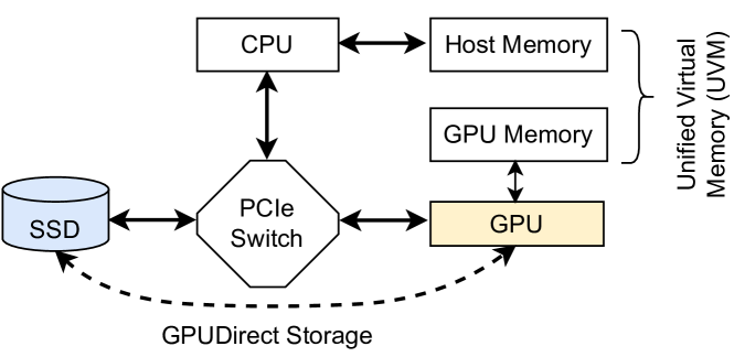
Figure 1. Modern GPU memory/storage architecture.

2.1. GPU Memory and Storage Architecture

We demonstrate the system architecture of modern GPU memory and storage in Figure 1. The GPU and storage devices like SSDs are connected with the host machine through the Peripheral Component Interconnect Express (PCIe) (pci, [n. d.]). While GPU has its on-board memory, the memory capacity is constrained by the DRAM scaling wall and the limited on-board space for memory packages (Zhang and Jung, 2020). Therefore, their memory cannot host the entire working set of large-scale deep learning workloads. To address this problem, GPUs follow the same way of managing memory/storage devices in CPU-centric computing, and use the storage device as a swapping disk. If a page requested by the GPU is not in its memory, a page fault will happen. And the GPU will inform the host to handle the page fault, load the page from the storage device, and move it to the GPU memory, causing significant data movement overhead.

2.2. Approaches to Scaling GPU Memory

Expand GPU memory with host memory. Compared to the GPU memory, the host machine usually equips a larger memory with limited bandwidth, making it a natural option for expanding GPU memory. While developers can manually swap the data between the host and GPU, modern GPUs make this procedure transparent with unified virtual memory (UVM) (Unified Memory for CUDA Beginners, [n. d.]; Unified CPU/GPU Memory Architecture Raises the Performance Bar, [n. d.]). UVM enables a unified and coherent virtual memory space between the host and GPU, so application data can be allocated to the space and accessed by host and GPU with shared virtual addresses. With the cooperation of GPU hardware and runtime, UVM maintains data consistency transparently and enables on-demand data migrations between the host and GPU at page granularity.

Upon accessing a UVM page absent in the GPU memory, a GPU page fault will be triggered to request a data migration from the host (Zheng et al., 2016; Allen and Ge, 2021). When the GPU memory is fully occupied, the least recently used pages are evicted from the GPU memory to the host memory. To improve the swapping efficiency, prior studies (Huang et al., 2020; Ganguly et al., 2019; Ren et al., 2021a; Hildebrand et al., 2020; Le et al., 2019; Jung et al., 2023; Rajbhandari et al., 2021; Awan et al., 2018) developed optimization techniques for improved data locality. However, GPU memory still cannot scale purely relying on the host memory to meet the increasing demands of deep learning workloads, especially those large ones.

Expand GPU memory with flash memory. An alternative approach is to expand GPU memory with SSDs, as shown in Figure 1. The rapidly shrinking process technology has allowed SSDs to boost their bandwidth and capacity by increasing the number of chips. However, the GPU has to communicate with the host CPU to access data on the SSD, which incurs significant performance overhead (Silberstein et al., 2013; Kim et al., 2014; Shahar et al., 2016). Most recently, NVIDIA’s GPUDirect Storage allows GPU to bypass the host CPU and directly access the SSD via the PCIe interface (GPUDirect Storage: A Direct Path Between Storage and GPU Memory, [n. d.]). AMD’s DirectGMA (AMD DirectGMA, [n. d.]) also enables a similar functionality.

However, current approaches of using flash memory to expand GPU memory are still suffering from suboptimal performance, as they cannot efficiently hide the slow flash accesses. A recent study proposed to offload intermediate data of DNN models to the SSD (Bae et al., 2021), and overlap the GPU processing with flash data accesses. However, due to the lack of rich semantic knowledge of tensors, there is still much space for improvement. In this paper, we conduct a characterization study of the semantic knowledge of tensors, and demonstrate the unexplored opportunities in $\S$3.

3. GPU Memory Characterizations

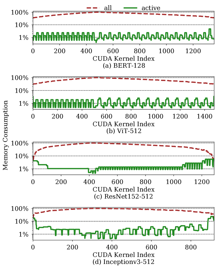
Figure 2. Memory consumption of all and active tensors (w.r.t. peak memory consumption in a single training iteration). CUDA kernel indexes are in execution order.

In this section, we first study the memory usage patterns of DNN training for representative real-world large models listed in Table 1. We analyze the DNN dataflow graph to extract useful DNN semantics and profile the execution of each CUDA kernel on an NVIDIA A100 GPU. For ease of discussion, we define that a tensor is active at a certain time if it is used by the currently executing kernel, or inactive otherwise. We summarize our findings as follows.

Small memory requirement of active tensors. We first study the total memory demand of a single training iteration. Figure 2 shows the amount of GPU memory required by active tensors and the total memory required during a training iteration. For most DNN models, active tensors only account for less than 10% (1% on average) of the total memory requirement. While the memory capacity required by the entire DNN can greatly exceed GPU memory, each layer only accounts for a small portion. For example, the largest kernel in our studied models occupies 5.7GB of memory, much smaller than the 40GB available memory of A100. This gives abundant opportunities to leverage the unused memory for preparing the tensors required by the next kernel, enabling efficient overlapping of GPU compute and memory swapping.

Observation (O1):  During DNN training, only a small portion of tensors are active and required in GPU DRAM. Most tensors are inactive and can be swapped out.

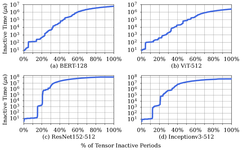
Figure 3. Distribution of tensor inactive period lengths.

Figure 4. The distribution of inactive periods of tensors having different sizes.

Long unused time of inactive tensors. To understand the memory usage pattern of inactive tensors, we study how long a tensor remains inactive. We define an inactive period as a time interval during which the tensor remains inactive until it is used by another kernel. Figure 3 shows the distribution of lengths of the inactive periods for all tensors. For CNN models (ResNet152 and Inceptionv3), more than 60% of the inactive periods last longer than $10^{7}$µs. For Transformer models (BERT and ViT), about 50% of the inactive periods last longer than $10^{5}$µs. This indicates that many tensors have inactive periods longer than the SSD latency (e.g., 20µs), which provides opportunities for us to swap out these tensors to external SSD devices with negligible performance penalties.

The long unused time of inactive tensors is the result of the temporally sparse tensor access pattern during DNN training. In a typical DNN dataflow graph, one tensor only needs to be used twice, one in the forward pass and the other in the backward pass, unless the tensor is involved in a branch or join layer. Although the dataflow graphs of some DNN models may have a complex topology consisting of multiple branches, joins, and unrolled loops, the overall dataflow still tends to be linear, so each tensor is only used for a few times.

Observation (O2):  During DNN training, many tensors stay inactive for a long time period. They can be safely swapped out before being needed again by any kernel.

Diversity of inactive tensors. Figure 4 shows that the inactive periods of tensors have diverse lengths (e.g., ranging from $\thicksim$10µs to 100s in Inceptionv3-512). The inactive tensors also have vastly different sizes (e.g., from less than 10KB to more than 2.7GB in Inceptionv3-512), and their distribution is quite sparse. In fact, over 60% to 80% of inactive periods are able to hide the swapping latency, indicating that we have sufficient opportunities to swap tensors.

When we decide to swap out a tensor, we can reduce the GPU memory consumption during the tensor’s inactive period. The diversity of inactive tensors introduces challenges to the swapping algorithm design, as different swapping decisions can have different benefits and I/O costs. To maximize the efficiency of memory swapping, it is important to choose those tensors that can reduce the memory usage by the largest amount, for the longest time, and with the lowest I/O cost.

Observation (O3):  Different swapping decisions impact GPU memory consumption differently in both time and space, given the different sizes and inactive period lengths of tensors. To maximize memory efficiency, we should swap out the most beneficial tensors.

Complexity of scheduling tensor swapping. In Figure 2, we observe that the memory consumption of a DNN program is not uniform throughout its entire execution. As we make tensor swapping decisions, the GPU memory consumption pattern also changes as tensors are swapped in or out at runtime. Moreover, each swap occupies bandwidth of GPU-Host and GPU-SSD communications. Consequently, the above complexities render a static policy ineffective for deciding which tensor should be evicted and what time this eviction should occur.

Observation (O4):  The GPU memory consumption changes throughout the DNN training process and is affected dynamically by tensor swapping decisions. Hence, a static tensor swapping policy is insufficient for finding a globally optimized swapping plan.

4. G10 Design

Figure 5. System architecture of G10.

4.1. System Overview

We show the G10 architecture in Figure 5. It has three major components: (1) a tensor vitality analyzer that quantifies the tensor size and liveness as we compile a DNN model ($\S$4.2); (2) a tensor migration scheduler for planning the tensor migrations in advance ($\S$4.3 and $\S$4.4); and (3) a unified memory system for simplifying GPU memory management and enabling transparent tensor migrations ($\S$4.5 and $\S$4.6).

Given a DNN model, G10’s tensor vitality analyzer will work with DNN compilers to track all the tensors and their dependencies, and quantify their sizes and lifetime (i.e., semantic knowledge of tensors). With these knowledge, the tensor migration scheduler will plan the optimized execution schemes of tensors, with the goal of maximally overlapping the GPU computation and tensor migrations. Identifying a globally optimized tensor migration plan is a dynamic optimization problem, as each tensor migration decision will affect subsequent decisions, due to its impact on the GPU memory pressure, and GPU-SSD and GPU-Host bandwidth utilizations. Therefore, we used a dynamic algorithm to iteratively find the best tensor candidates for eviction and prefetching. After that, G10 adds the eviction and prefetch instructions into the compiled program. GPU will execute these instructions at runtime with the unified GPU memory and storage architecture. As the GPU memory, host memory, and SSD are combined into a unified space, the tensor migrations are fully transparent to developers and DNN workloads. We will describe each component of G10 as follows.

4.2. Tensor Vitality Analysis

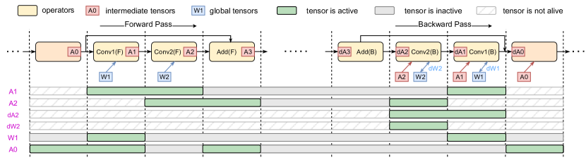
Figure 6. An example of tensor vitality analysis for a residual basic block. Operators in forward propagation and in backward propagation are marked as Op(F) and Op(B), respectively. Ax and Wx are activation tensors and weight tensors, respectively. dAx and dWx are the corresponding gradient tensors.

Identifying global tensors and intermediate tensors. We first categorize the tensors based on their lifetimes in a DNN training iteration (i.e., one round of forward and backward propagation). As shown in Figure 6, a global tensor such as model weights (e.g., W1) is used across multiple training iterations. It will be allocated in the unified memory space at the beginning of the DNN program. An intermediate tensor, such as the activation and gradient (e.g., A1 and dA2), is used within one iteration. We define the tensor as born the first time when it was used, and as dead after the last time it was used. Intermediate tensors can be deallocated after their deaths to free up GPU memory.

Identifying tensor inactive time periods. When an operator is being executed on GPU, both its input and output tensors are active, and should be present in GPU memory. Otherwise, a tensor is inactive, if it is not being used by the currently executing kernel and is not yet dead. We define an inactive time period of a tensor as the period during which the tensor is inactive and not dead (i.e., it is not being used right now but will be used in the future). For a complex DNN program, a tensor may have multiple inactive time periods and can be swapped in and out multiple times (e.g., W1 and A0). Both global and intermediate tensors can be inactive, and the inactive time period of a global tensor may span across two consecutive training iterations. For example, W1 turns inactive during the backward pass of the current iteration, and it becomes active again in the forward pass of the next.

The inactive time periods of all tensors indicate when a tensor is safe to be migrated out and when it must be migrated back. As DNN programs have predictable performance and dataflow patterns, G10 performs offline compile-time profiling, and uses the execution times of the GPU kernels to estimate the lengths of the inactive time periods. Using the tensor sizes, the storage bandwidth, and the GPU-Host bandwidth, G10 estimates the eviction and prefetch overheads of each tensor. G10 then leverages all the inactive time periods to generate a globally optimized execution plan.

4.3. Smart Tensor Eviction

Input: $gpu\_cap\leftarrow$ the GPU on-board memory capacity

            $tensors\leftarrow$ the list of all intermediate tensors

            $periods\leftarrow$ the list of all tensor inactive periods

Output: A list of G10 tensor migration instructions

1 Function $EvictionScheduling$($gpu\_cap,\ tensors,\ periods$):

2       for i = 0; i $<$ periods.size; i++ do

3             if $max(mem\_pressure)<gpu\_cap$ then

4                   break

5             sort $periods$ by critical_mem_pressure_reduction)

6             if $periods[0].critical\_mem\_pressure\_reduction>0$ then

7                   $t\_r\leftarrow$ periods[0].start_time

8                   $t\_s\leftarrow$ periods[0].tensor_size / BW_SSD

9                   if (to_ssd_traffic is full during $t\_r$ to $t\_r$ + $t\_s$) then

10                         if host mem isn’t full during periods[0] then

11                               schedule pre-eviction(periods[0].tensor, host) at $t\_r$

12                               periods.erase(0)

13                               update memory pressure and I/O traffic

14                               continue

15                              

16                        

17                   schedule pre-eviction(periods[0].tensor, SSD) at $t\_r$

18                   update memory pressure and I/O traffic

19                   periods.erase(0)

20                  

21            

22      

Algorithm 1 Smart Tensor Eviction Algorithm.

To generate a globally optimized migration plan, the smart tensor eviction algorithm must address the following challenges. First, we must utilize the limited GPU on-board memory to store the most beneficial tensors. As tensors have different sizes and inactive period lengths, they contribute different degrees of GPU memory pressure. Thus, evicting some tensors (e.g., large tensors with long inactive periods) yields more benefits in reducing GPU memory pressure. Second, we must consider both SSD and host memory as potential migration destinations, as they provide different bandwidths, capacities, and different migration overheads. Ideally, we aim to exploit both the high migration bandwidth of host memory and the large capacity of SSD. Third, we should best utilize the available migration bandwidth, as DNN workloads are mostly bandwidth-sensitive. The algorithm should also choose the best timings for tensor migrations.

To this end, we propose a smart eviction scheduling algorithm that iteratively finds the best eviction candidates (i.e., tensor inactive periods) in each training iteration at compile time. The algorithm tracks the GPU memory consumption and the migration bandwidth utilization to evaluate potential benefits of an eviction. We describe its key ideas as follows.

Selecting eviction candidates. To determine the best eviction candidate, we holistically estimate the benefit and cost of each eviction candidate. To quantify the eviction benefit, we define the GPU memory pressure as the total size of non-evicted tensors in GPU memory at time $T$. If the pressure exceeds the GPU memory capacity at any time, hardware page faults will occur and harm the performance. Thus, the eviction candidate is beneficial if it reduces the memory pressure exceeding the capacity, as shown in the shaded area in Figure 7(2). The area of the shaded area quantifies the benefit of eviction: a larger shaded area implies a larger tensor or longer inactive period. Using this criterion, G10 sorts the inactive periods of all tensors to find the best eviction candidates.

The cost of an eviction candidate is quantified as the sum of eviction and prefetch latencies of this tensor. Thus, G10 favors migrations with low migration latencies, as other migrations may exclusively occupy the interconnect for a longer time and cause contentions, as shown in Figure 7(3).

For example, in Figure 7(1), we designate the best candidate as tensor $X$’s inactive period $A$. By evicting $X$ during $A$, we reduce the most pressure over the capacity limit (i.e., largest shaded area in Figure 7(2)) while causing the least I/O bandwidth overhead (shown as + in Figure 7(3)). Specifically, it has highest benefit-cost ratio of $\leavevmode\hbox to8.5pt{\vbox to8.5pt{\text{[drawing]}}}/(\leavevmode\hbox to8.5pt{\vbox to8.5pt{\text{[drawing]}}}+\leavevmode\hbox to8.5pt{\vbox to8.5pt{\text{[drawing]}}})$.

Figure 7. An example of state transition in G10’s smart migration scheduling algorithm.

Choosing eviction destination. After selecting the candidate tensors, we need to decide between two potential migration destinations, SSD and host memory, as they provide different capacities and bandwidths. In G10, we always attempt to evict tensors to the SSD first, due to its large capacity. In contrast, host memory only offers a limited memory capacity, and thus naïvly evicting to host memory easily consumes up the capacity, and falls back to evicting to SSD eventually. However, in some cases, we still want to leverage the valuable host memory for our tensor migration. Compared to the SSD, the host DRAM offers much higher access bandwidth. Thus, we only evict a tensor to host memory, when the SSD traffic is under high pressure, as shown in line 7-17 in Algorithm 1. In this way, G10 exploits the large SSD capacity when its bandwidth is sufficient, and utilizes the high migration bandwidth of GPU-Host when the SSD bandwidth is saturated.

Smart Tensor Eviction Scheduling. We describe the end-to-end procedure of G10’s smart tensor eviction scheduling algorithm in Algorithm 1. To generate an optimized migration plan, it iteratively searches for the best eviction candidate, until the GPU memory pressure is below the capacity limit or there are no more beneficial eviction candidates.

The algorithm tracks the three global states throughout the search process: (1) a set of inactive periods, (2) the estimated memory pressure versus time, and (3) the estimated bandwidth utilizations. In each iteration of the algorithm, it selects one eviction candidate, chooses where to evict this tensor as described above, and updates the three states accordingly.

4.4. Smart Tensor Prefetching

Figure 8. An example of scheduling prefetch time for one evicted inactive tensor.

To maximize memory pressure suppression, the smart tensor eviction algorithm assumes the prefetch to be performed at the latest time that does not cause data idleness, which is defined as the latest safe prefetch time. However, to ensure that each prefetch completes exactly before the respective tensor turns active, the algorithm needs a perfect estimation on inactive period lengths and I/O traffic status. Thus, inaccurate estimation of inactive period length or I/O traffic status will incur stalls under this default prefetch policy.

Our insight is that for most DNN programs, the GPU memory pressure is under the capacity limit after scheduling the evictions. As shown in Figure 8, the GPU memory pressure, presented as the black curve, is under the GPU capacity over time. The naïve prefetch policy does not fully utilize the remaining GPU memory.

Based on our insight, G10 applies a smart prefetching algorithm that prefetches evicted inactive tensors eagerly to further tolerate imperfect migration decisions. G10 sorts all the evicted tensor inactive periods in the order of their latest safe prefetch time. G10 then traverses all evicted tensor inactive periods in order and reschedules their prefetch beforehand if possible. Figure 8 shows an example. For one evicted inactive period $i$ with the latest safe prefetch time $t_{i}$, the algorithm searches backward from time $t_{i}$ until reaching the earliest time $t_{i}^{\prime}$, when GPU can hold the entire tensor safely with the available space. In other words, the algorithm selects a time $t_{i}^{\prime}$ at which placing this tensor on GPU will not exceed GPU memory capacity. Therefore, the algorithm schedules the prefetch for this tensor at $t_{i}^{\prime}$, and the GPU memory pressure curve between time $t_{i}^{\prime}$ and $t_{i}$ is updated. If there is not such an optimization opportunity, the prefetch instruction will still be scheduled at time $t_{i}$.

Code Instrumentation. To enable smart data migration, G10 utilizes deep learning comilers to automatically insert the following instructions into the generated GPU program: (1) g10_prefetch(vaddr, size), which fetches a tensor into GPU memory; (2) g10_pre_evict (vaddr, size, target_loc), which evicts a tensor from GPU memory to the SSD or host memory; (3) g10_alloc(**ptr, size), which allocates a buffer on the GPU memory asynchronously; (4) g10_free(*ptr), which frees the buffer asynchronously. We show an example of instrumented GPU program in Figure 9. We will further discuss these instructions in $\S$4.6.

frame=tb, language=C, aboveskip=3mm, belowskip=3mm, showstringspaces=false, columns=flexible, basicstyle=, numbers=left, numbersep=5pt, numberstyle=, keywordstyle=, commentstyle=, stringstyle=, breaklines=true, breakatwhitespace=true, tabsize=4, classoffset=0, morekeywords=g10_alloc, g10_free, g10_prefetch, g10_pre_evict, keywordstyle=, classoffset=1, morekeywords=tensor2914, keywordstyle=, classoffset=2, morekeywords=tensor22, keywordstyle=, classoffset=3, morekeywords=tensor23, keywordstyle=, classoffset=4, morekeywords=tensor20, keywordstyle=, classoffset=5, morekeywords=forward_conv2d_l4, keywordstyle=,

⬇

…

g10_alloc(tensor20, 40960);

g10_prefetch(tensor23, 40960);

// Kernel 2 ReLU(input, output)

forward_ReLU_l2(tensor5, tensor5);

…

g10_alloc(&tensor22, 77073360);

g10_alloc(&tensor2914, 4110417920);

// Kernel 3 MaxPool2d(input, output)

forward_MaxPool2d_l3(tensor5, tensor20);

…

// Kernel 4 Conv2d(input, output, filter, workspace)

forward_conv2d_l4(tensor20, tensor22, tensor23, tensor2914);

g10_free(tensor2914);

g10_pre_evict(tensor23, 40960, SSD);

…

// Kernel 5 BatchNorm2d(…)

forward_BatchNorm2d_l5(tensor22, tensor28, tensor38, tensor39, tensor30, tensor31, tensor32, tensor33);

…

Figure 9. An example of instrumented GPU program.

4.5. Unified GPU Memory and Storage

The diversified memory and storage hierarchy (i.e., GPU memory, host memory, and SSD) inevitably increases the complexity of GPU memory management, and makes it challenging for G10 to track the memory locations for each tensor. To address this challenge, we develop a unified memory space. Therefore, G10 can plan the tensor migration schemes using virtual addresses, the runtime system will rely on the unified virtual memory to conduct the address translation, and identify the physical locations of tensors transparently.

Prior studies (Huang et al., 2015; Abulila et al., 2019) proposed the unified address translation for memory-mapped SSDs, which combines the address mapping of SSDs into the page table of the virtual memory. Therefore, the page table entries can directly point to the physical flash addresses. Although GPU provides the unified virtual memory (UVM) to manage the host memory and GPU memory in a unified space (Agarwal et al., 2015; Ausavarungnirun et al., 2017; Hao et al., 2017; Kim et al., 2020), current GPU UVM does not support flash memory.

G10 integrates the GPU memory, host memory, and flash memory into a unified memory space for enabling transparent tensor migrations. With unified memory, all tensors are managed at the regular 4KB page granularity. For the tensors whose size is less than 4KB, G10 will compact them in a page to minimize the memory fragmentation across different memory types. As the GPU and host interact with the SSD at the regular page granularity, the I/O amplification of the SSD will not be worse than commodity SSDs.

With the UVM extension, G10 has a unified address translation layer in the memory manager, where the flash address mappings in the flash translation layer have been integrated into the page table of the GPU UVM. In this case, the page table entry (PTE) will either point to an address in host memory or GPU memory or flash memory. G10 allows the SSD controller to update the page table entries (PTEs), when garbage collection (GC) of the SSD moves valid flash pages to a new flash block. G10 relies on the existing UVM supports to maintain the consistency of the host-side unified page table and GPU-side local page table, as well as the TLBs. As G10 migrates tensors among GPU memory, host memory, and SSD at page granularity, the corresponding PTEs and TLBs will also be updated with the new page address. Since the PTE and its corresponding TLB are always updated, the unified memory system handles address translations and paging to load data from SSD or host memory to the GPU memory.

The UVM extension simplifies the programmability and enables transparent tensor migration. Its page fault handling mechanism may incur extra performance overhead. However, the smart tensor migration mechanism in G10 minimizes unexpected page faults and data migrations, which makes the UVM extension an appealing feature (see Figure 11).

4.6. Tensor Migration with Extended UVM

Figure 10. The workflow of runtime migrations in G10.

G10 supports smart tensor migration with the extended UVM ($\S$4.5). It extends the device UVM driver to implement the smart migration handler on the host. We show the workflow of tensor migration in Figure 10. Upon executing g10_pre_evict(vaddr, size, target_loc), CUDA runtime will send an exception to the migration handler on the host side. The migration handler will initiate the migration of the corresponding tensor, and migrate the tensor to the specified location target_loc via the DMA engine. Note that G10 will rely on the unified memory system for the address translation for vaddr, and use the size to decide how many pages it will migrate. Upon executing g10_prefetch(vaddr, size), the tensor migration handler will access the unified memory with vaddr. It will initiate the prefetching process and request the GPU DMA engine to fetch the tensor from the host memory or SSD.

As shown in Figure 10, for tensor evictions and prefetching, G10 will rely on the unified page table to identify the physical locations of tensors ( ). For pre-evictions, G10 will look up the GPU page to be evicted. After that, the migration metadata will be stored in corresponding Migration Metadata Queues ( ). The Migration Arbiter will select several page migrations to form the next migration batch and store them in the Transfer Sets ( ). During this procedure, The G10 driver will also communicate with GPU to allocate GPU memory on demand. The migrations in the Transfer Sets will be batched periodically, the corresponding SSD-GPU data transfer will be handled by the Direct Storage Access (DSA) process, and CPU-GPU data transfer will be handled by the DMA process ( ). After the data migrations, the unified page table and corresponding TLB entries will be updated ( ).

G10 fully utilizes the GPU-Host bandwidth and storage bandwidth with data batching. Migration Arbiter applies different priorities to different migration queues (e.g., page faults have the highest priority). G10 will calculate the batch number in the next round to fully saturate the bandwidth.

5. Implementation details

Tensor vitality analyzer. The tensor vitality analyzer is a static analysis tool, which is compatible with the deep learning compiler PyTorch. The analyzer takes a DNN model and the profiled execution time of each kernel as inputs. After the static analysis ($\S$4.2), it generates instrumented CUDA programs. We take the instrumented program into the simulator framework (see below) to simulate the entire G10 system.

Simulator framework. To efficiently simulate the executions of diverse DNN models, we first run these real models on a real A100 GPU and trace the execution of all kernels. We build a simulation framework based on UVMSmart(Ganguly et al., 2019) and GPGPU-Sim(Lew et al., 2019) to simulate the UVM, including the GPU page fault handling, data migration, and address translation. Our simulator supports taking the execution traces as input, so it can replay the kernel traces. we believe our simulation framework reasonably models the actual execution of DNN models, especially considering it replays real kernel traces collected on a real GPU.

We focus on the address translation and coherency support for the unified page tables. We modeled the latency overheads caused by the host page fault handler, the interaction between the GPU and CPU for the page fault handler, and page table walks, inside our timing model for accurate measurements.

When incorporating SSD into the UVM system, we follow the approach described in prior studies (Abulila et al., 2019). We rely on the host page fault handing mechanism to do the address translation. Upon access to pages that do not reside in GPU memory, the GPU page fault handler will raise an interrupt to the host, and the host is responsible for moving data. To simulate the SSD internals and capture their activities, such as garbage collection (GC) and flash chip accesses, in our evaluation, we developed an SSD simulator based on SSD-Sim(Agrawal et al., 2008) and integrated it into our simulator framework. Therefore, as we measure the overall system performance during the experiments, the internal SSD activities are considered.

Table 1. Evaluated DNN models and datasets.

Model	# Kernels	Source	Dataset
BERT (Devlin et al., 2018)	1368	Hugging Face	CoLA
ViT (Dosovitskiy et al., 2021)	1435	Hugging Face	ImageNet
Inceptionv3 (Szegedy et al., 2016)	740	Pytorch Examples	ImageNet
ResNet152 (He et al., 2016)	1298	Pytorch Examples	ImageNet
SENet154 (Hu et al., 2018)	2318	Pytorch Examples	ImageNet

Table 2. System Configuration.

CPU Main Memory	128GB DDR4
GPU	NVIDIA A100
GPU Memory	40GB HBM2e
Page Size	4KB
SSD Read/Write Bandwidth	3.2/3.0 GB/s
SSD Read/Write Latency	20/16 $\mu$s
SSD Capacity	3.2 TB
Interconnect	PCIe Gen3 x16
GPU Page Fault Handling Latency	45 $\mu$s

6. Discussion and Future Work

Multi-GPU support. G10 can be simply extended to effectively support multiple GPUs for three reasons. First, as multiple GPUs share SSDs, and each GPU can run independently, we can deploy the smart tensor migration mechanism of G10 on each GPU. Therefore, each GPU will make its own decisions on the tensor migrations. Second, current UVM has supported multiple GPUs, which has created a unified memory space across the host memory and all GPUs’ memory. The UVM extension of G10 supports multiple GPUs by integrating the shared flash memory space into the existing UVM as discussed in §4.5. Third, as we increase the number of GPUs, we may want to increase the number of SSDs for increasing aggregated storage bandwidth. Since the SSD array (e.g., using RAID) is shared by multiple GPUs, G10 will treat the SSD array as a shared flash memory space and integrate it into the UVM. Our evaluation (§7.5) will conduct the sensitivity analysis as we increase the number of SSDs. We wish to explore the multi-GPU support as future work.

7. Evaluation

We show that (1) G10 outperforms state-of-the-art designs by up to 1.75$\times$ for training large DNN models that exceed GPU on-board memory capacity ($\S$7.2); (2) G10 supports larger batch sizes with better performance than other designs ($\S$7.3); (3) G10 saves host memory capacity with negligible performance degradation ($\S$7.4); (4) G10 improves DNN training performance with different hardware settings ($\S$7.5); (5) G10’s scheduling algorithm is resilient against profiling errors ($\S$7.6); (6) G10 has negligible negative impact on the SSD lifetime ($\S$7.7).

Figure 11. DNN training throughput normalized to the ideal performance. B is batch size. M is the total memory consumption of the DNN w.r.t. GPU memory capacity.

7.1. Experimental Setup

We evaluate G10 with diverse DNN models in Table 1, including transformer-based models (BERT and ViT) and CNNs (ResNet, Inceptionv3, and SENet). The models are retrieved from PyTorch examples (PyTorch, 2023. PyTorch Examples, [n. d.]) and the Hugging Face public repositories (Huggingface, 2023. Transformers., [n. d.]), and the training datasets include CoLA (Warstadt et al., 2018) and ImageNet (Krizhevsky et al., 2012). We use FP32 format for the tensor representation. We vary the batch size for each model to study the impact of different memory demands.

System configuration. Table 2 shows the hardware configuration of our experimental testbed. We set the SSD parameters based on Samsung Z-NAND SSD (Samsung, [n. d.]). The host memory, GPU, and SSD are connected with a PCIe interconnect that can deliver a bandwidth of 15.754 GB/s bidirectionally. We model the UVM system following prior works (Ganguly et al., 2019; Zheng et al., 2016).

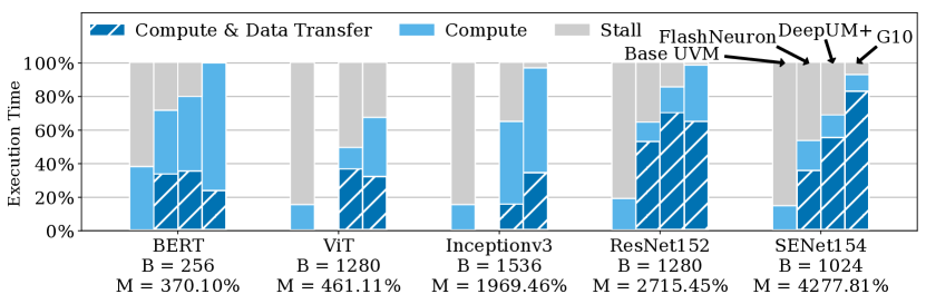
Figure 12. Execution time breakdown of training (left to right: Base UVM, FlashNeuron, DeepUM+, G10).

We compare G10 with several state-of-the-art GPU memory-expanding solutions: DeepUM+(Jung et al., 2023) and FlashNeuron(Bae et al., 2021). We also evaluate G10 with different host memory capacities. As hardware capabilities evolve over time, we conduct sensitivity analysis with different SSD bandwidths. To summarize, we compare G10 against the following baseline designs:

• Ideal: a GPU with infinite on-board memory, which gives the theoretically best performance.

• Base UVM: the basic GPU-CPU-SSD UVM system with only on-demand page migrations via page faults.

• DeepUM+: a UVM system using a correlation-based prefetcher to prefetch data to the GPU memory. We extend the original GPU-CPU-based DeepUM design (Jung et al., 2023) to support SSDs. Upon a GPU page eviction, if the CPU memory is full, DeepUM+ can still evict the page to the SSD.

• FlashNeuron (Bae et al., 2021): a DNN training library using direct GPU-SSD communication to selectively swap intermediate tensors (instead of all tensors) to the SSD. Since FlashNeuron worked in a traditional non-UVM style, we used FlashNeuron’s memory manager for fair comparison.

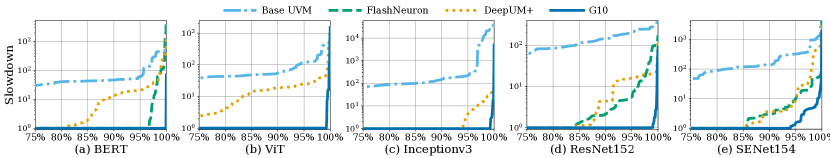
Figure 13. Distribution of kernel execution time slowdown normalized to ideal performance (lower is better).

7.2. End-to-end Performance

We show the end-to-end DNN training throughput of different benchmarks in Figure 11 On average, G10 outperforms FlashNeuron by 1.56$\times$ and DeepUM+ by 1.31$\times$. Compared to the ideal system with infinite GPU memory, G10 unleashes 90.3% of the ideal performance using limited GPU memory.

DNN training throughput. As shown in Figure 11, Base UVM performs 4.55$\times$ worse than the ideal, due to the significant page fault overhead. With heuristic-based tensor eviction and prefetching, FlashNeuron and DeepVM+ improve the performance over Base UVM by 2.46$\times$ and 3.12$\times$, respectively. However, both of them are still much slower than the ideal performance. Although DeepUM+ supports DNN models with large memory demands, its correlation-based prefetching mechanism cannot capture rich DNN semantics.

G10 outperforms FlashNeuron and DeepVM+ by up to 1.75$\times$, which demonstrates the effectiveness of the smart tensor migration algorithm in capturing DNN semantics. For most benchmarks, G10 achieves nearly ideal performance by exploiting the deterministic dataflow of DNN workloads and best utilizing the limited I/O bandwidth. The only exception is ViT, which has high migration I/O bandwidth demand when the batch size is large.

To further understand the benefits of G10, we gradually enable the features of G10. Therefore, we have (1) G10-GDS that only supports tensor migrations between GPU and SSD; (2) G10-Host that enables tensor migrations among GPU, host, and SSD; and (3) G10 that extends G10-Host by having the UVM extension which unifies the GPU memory, host memory, and SSD ($\S$4.5). As shown in Figure 11, G10-GDS outperforms existing solutions for most DNN workloads, because of its smart tensor migrations. G10-Host further improves the performance as it utilizes the host memory. For ResNet152 workload, G10-GDS does not perform better than DeepUM+, because G10-GDS can only migrate tensors between GPU and SSD. However, by enabling tensor migrations between GPU and host, G10-Host outperforms DeepUM+ by 1.23$\times$. With UVM extension enabled, G10 further improves the performance, due to the reduced software overhead of accessing flash pages and handling page faults.

Execution time breakdown. The performance benefit of G10 comes from the better overlapping between computation and memory swapping. Figure 12 shows the percentage of time during which tensor migrations perfectly overlap with GPU computation, and the percentage of time when tensor migrations stall GPU computation. Compared to all other designs, G10 has the least stall time, since it generates a better swapping schedule than other designs.

Figure 13 further shows how many kernels are stalled by tensor swapping. For Base UVM, more than half of the kernels (truncated in the figure) suffer page fault overhead. FlashNeuron and DeepUM+ reduce the number of affected kernels, but both designs still cause significant slowdown to many kernels (4%–30% of kernels). With G10, only 1%–6% of kernels perform worse than the ideal case.

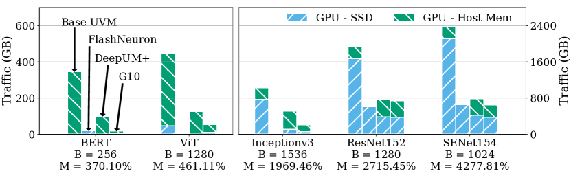
Figure 14. Tensor migration traffic breakdown.

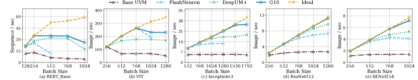
Figure 15. Training throughput with varying batch sizes.

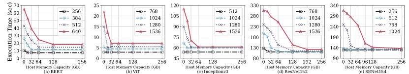
Figure 16. Execution time as we vary the host memory capacity.

Tensor migration traffic. To understand how G10 utilizes the available I/O bandwidth, we show the total migration traffic of GPU-SSD and GPU-Host in Figure 14. Due to the inefficiency of heuristic-based migration policies (e.g., LRU policy and linear selection(Bae et al., 2021)), Base UVMand DeepUM+schedule more tensor evictions than necessary. On the contrary, FlashNeurondoes not schedule a sufficient number of evictions as it does not swap weight tensors, so it cannot reserve enough space for future tensors in a timely manner.

We also observe that a small amount of host memory plays a critical role for G10 to tolerate tensors that have high migration bandwidth demands. Particularly, transformer models (BERT and ViT) are more bandwidth-intensive, so G10 directs most of their migration traffic to the host memory. CNN models are more compute-intensive, thus, the SSD bandwidth can sustain more than half of the migration traffic. By fully utilizing the available bandwidth, G10 unleashes the potential of the GPU-CPU-SSD unified memory.

7.3. Performance with Varying Batch Size

As batch size varies, the performance of G10 is always the closest to ideal among all the designs. In Figure 15, while most designs achieve the ideal performance when the batch sizes are small and the memory demand is low, G10 can tolerate larger batch sizes and higher memory demands. With larger batch sizes, more tensors must be swapped with the limited I/O bandwidth. Thus, it is more crucial to make smart migration decisions to hide the migration latency and avoid stalling future kernels. Despite significantly outperforming Base UVM, DeepUM+, and FlashNeuron quickly fall behind the ideal performance as batch size increases, due to the sub-optimal swapping policies. G10 still timely delivers required data to the active kernels under strict capacity and bandwidth limitations in most cases, thanks to its intelligent tensor migrations. In general, G10 outperforms FlashNeuron and DeepUM+ by up to 2.67$\times$ and 1.45$\times$, respectively.

As batch size continues to increase, the performance of all designs eventually degrades, but G10 still outperforms all other designs. If the total memory consumption of the current and the next kernel exceeds GPU memory capacity, data required by the next kernel cannot be ready in GPU before the kernel starts. Thus, the next kernel inevitably stalls due to poor overlapping between computation and data transfer.

7.4. Impact of Varying Host Memory Capacity

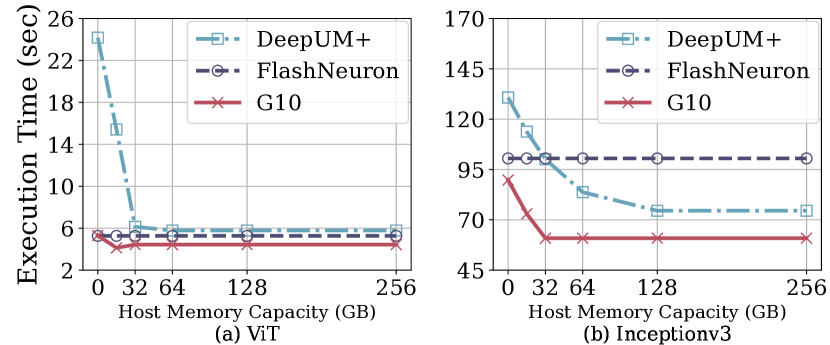
Figure 17. Performance comparison of G10, DeepUM+, and FlashNeuron with different host memory capacity.

While using the cost-efficient SSD to expand GPU memory capacity, G10 also leverages the host memory bandwidth to compensate for tensors that cannot be swapped into and back from the SSD within their inactive periods. Since most tensors do not require high migration bandwidth (Figure 4), G10 only needs a small amount of host memory to tolerate them. Figure 16 shows G10’s performance with different host memory capacities. For most DNN models with small batch sizes, 32GB of host memory is sufficient for G10 to fully utilize the migration bandwidth between the host and GPU. The host memory capacity demand grows linearly with the batch size, as the sizes of the migrated tensors grow linearly.

As we vary the host memory capacity, we also compare G10 with DeepUM+ and FlashNeuron. We use two representative models: ViT (transformer) with the batch size of 1024 and Inceptionv3 (CNN) with the batch size of 1280. We show the results in Figure 17. When there is no host memory, G10 outperforms DeepUM+ and FlashNeuron by 2.58$\times$ and 1.04$\times$ on average, respectively. This is because DeepUM+ relies on conventional GPU UVM and incurs a significant number of page faults. As we increase the host memory capacity, the performance of DeepUM+ is improved, however, it still performs 1.26$\times$ worse than G10. As FlashNeuron fully relies on GPUDirect Storage and does not use host memory, its performance is barely affected as we vary the host memory capacity. Because of smart data migrations, G10 always performs better than FlashNeuron (1.33$\times$ on average).

7.5. Impact of Varying SSD Bandwidth

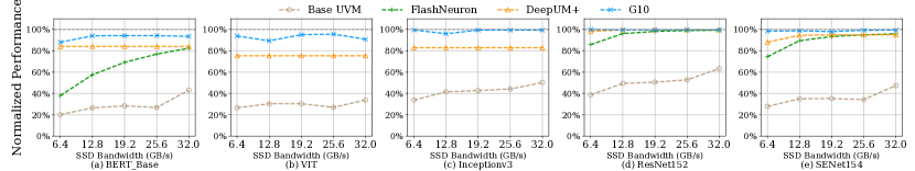
Figure 18. Performance with varying SSD bandwidth (normalized to ideal).

We now examine G10 with different SSD bandwidths (e.g., stacking multiple SSDs or using a higher-end SSD). For increased bandwidths, we assume the interconnect is PCIe 4.0 x16 (32 GB/s). In Figure 18, G10 outperforms all other designs regardless of the SSD bandwidth. For all benchmarks, 1 to 4 SSDs (up to 12.8 GB/s) are sufficient for G10 to achieve 90% to 100% of the ideal performance. BERT and ViT fail to attain the ideal performance because they are bottlenecked by the interconnect bandwidth (i.e., always swapping to host still cannot satisfy the bandwidth requirement). G10 exploits the high migration bandwidth of the host memory while best utilizing the SSD to reduce host memory pressure ($\S$7.4). In contrast, even with enough SSDs to saturate the interconnect bandwidth, FlashNeuronand DeepUM+still only achieve 70%-80% of ideal performance for BERT and ViT.

7.6. Impact of Profiling Errors

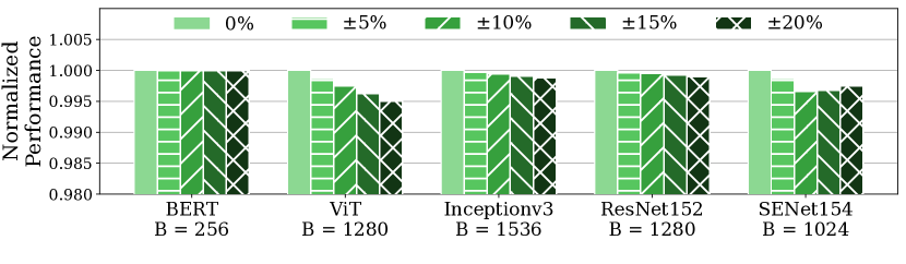
Figure 19. Performance of G10 under various degrees of kernel timing prediction errors (normalized to no error).

To understand the robustness of G10’s scheduling algorithm against profiling errors, we add random noises to the execution time of each kernel in our simulator. Figure 19 shows the performance of G10 with various degrees of profiling errors. For all benchmarks, the performance degradation is under 0.5% even when the profiling error is $\pm$20%. The profiling errors only affect the estimation of tensor inactive period lengths. G10 tolerates such errors by eagerly prefetching a tensor before it is used ($\S$4.4). In most cases, the early prefetch can tolerate the profiling inaccuracy.

7.7. Impact on SSD Lifetime

As reported in the released datasheet of Samsung Z-SSD SZ985(Samsung, [n. d.]), its device endurance is 30 Drive Writes Per Day (DWPD) for five years. According to our study, DNN workloads incur almost 50% writes and 50% reads. In this case, the SSD lifetime of G10 would be 30 DWPD * 1825 days (5 years) * 3.2TB / 3 GB/s * 2 = 3.7 years, when it is used continuously. Considering DNN workloads are data intensive and a commodity SSD usually lasts 3-5 years, the impact on SSD lifetime is not much of a concern. Based on Figure 14, we further break down the traffic into reads and writes. G10 incurs 1.37$\times$ and 2.20$\times$ less writes than DeepUM+ and FlashNeuron, respectively. As SSD lifetime is affected by the write traffic, G10 can achieve improved lifetime than state-of-the-art solutions.

8. Related Work

GPU memory wall. DNN workloads are heavily using GPUs. They rely on GPU memory and host memory to host their working sets. However, due to the limited capacity, they cannot host large models (Eisenman et al., 2019; Abadi et al., 2016; Kwon and Rhu, 2018; Chen et al., 2014; Peng et al., 2018). An alternative approach is to bring Flash closer to GPUs, such as GPUDirect Storage (GPUDirect Storage: A Direct Path Between Storage and GPU Memory, [n. d.]), ZnG (Zhang and Jung, 2020; Zhang et al., 2019), and AMD’s SSG (The World’s First GPU to Break the Terabyte Memory Barrier, [n. d.]; Examining AMD Radeon Pro SSG: How NAND Changes the GPU Game, [n. d.]). ZnG replaced GPU memory with flash chips and hard coded the flash addresses in the GPU MMU (Zhang and Jung, 2020). SSG and GPUDirect Storage enable GPU to directly communicate with SSDs via the PCIe interface (Examining AMD Radeon Pro SSG: How NAND Changes the GPU Game, [n. d.]). Unfortunately, their performance is bottlenecked by the PCIe bandwidth. In this paper, we develop a unified GPU memory system, and best utilize tensor behaviors to overcome the bottlenecks of slow memories.

New memory technologies. To overcome the memory scaling wall, researchers have been mostly focused on developing scalable memory technologies (Raoux et al., 2008; Loh, 2008; Zhao et al., 2013). For instance, HBM (High Bandwidth Memory, [n. d.]; AMD High Bandwidth Memory, [n. d.]) was produced to meet the bandwidth requirement of accelerators, but their capacity is still limited. Intel released its Optane persistent memory (Intel, 2018), and Samsung released its ultra-low latency SSDs (Samsung Z-NAND, [n. d.]). G10 is compatible with the new and emerging memory and storage devices, it leverages low-cost memories to scale the GPU memory while reaching near-to-ideal performance.

Unified memory and storage. Prior studies showed that SSDs can be used as memory via memory-mapped interface (Huang et al., 2015; Abulila et al., 2019; Saxena and Swift, 2010; Zhang et al., 2012; Badam et al., 2013; Josephson et al., 2010; Caulfield et al., 2009). However, they were designed for CPU-centric computing and cannot be directly applied to GPUs. NVIDIA and AMD have been supporting UVM in their GPU products by enabling unified memory between the host and GPU (Unified Memory for CUDA Beginners, [n. d.]; Unified CPU/GPU Memory Architecture Raises the Performance Bar, [n. d.]). G10 advances the architecture and integrates flash memories into the unified memory space. To optimize data movements between the host and GPU memory, prior studies (Huang et al., 2020; Ganguly et al., 2019; Ren et al., 2021a; Hildebrand et al., 2020; Jung et al., 2023; Rajbhandari et al., 2021) explored data localities of DNN workloads. G10 shares the same purpose with them. However, different from the studies like ZeRO series(Rajbhandari et al., 2021, 2020; Ren et al., 2021b) that offload tensors at a coarse (DNN layer) granularity, G10 enables tensor migrations at page granularity, and develops an active-time-aware tensor migration scheme.

9. Conclusion

We present G10, a unified GPU memory and storage architecture for scaling deep learning workloads. G10 is driven by our observation that the predictable tensor behaviors offer sufficient opportunities for G10 to make smart data migrations. Thus, we can overlap the GPU computation and flash accesses. With diverse DNN training workloads, we show that G10 can achieve near-ideal performance.

frame=tb, language=bash, aboveskip=3mm, belowskip=3mm, showstringspaces=false, columns=flexible, basicstyle=, numbers=left, numbersep=5pt, numberstyle=, keywordstyle=, commentstyle=, stringstyle=, breaklines=true, breakatwhitespace=true, tabsize=4, classoffset=0, morekeywords=apt, pip3, make, cd, wget, keywordstyle=,

Appendix A Artifact Appendix

A.1. Abstract

We implement G10 by building our own simulation framework described in ($\S$5). In this artifact, we provide the source code of G10 and necessary instructions to reproduce key performance results (Figure 2-4 in $\S$3 and Figure 11-19 in $\S$7).

The artifact can be executed on any x86 machine with at least 30 GB of main memory and at least 120 GB of disk space. We strongly recommend running the artifact on a workstation with multi-cores and at least 128 GB memory.

A.2. Artifact Checklist (Meta-Information)

• Algorithm: Tensor Vitality Analysis and Smart Tensor Migration Scheduling Algorithm.

• Compilation: GCC 9.4.0 or newer versions.

• Neural Network Models: BERT, ViT, ResNet, Inceptionv3, SENet. Their traces are included in the repo.

• Run-time environment: Ubuntu 18.04 or newer versions.

• Metrics: Execution time, training throughput, and migration traffic.

• Output: Files and graphs, expected results included in the repo.

• Experiments: Generate experiments using supplied scripts.

• How much disk space required (approximately): 120 GB

• How much time is needed to prepare workflow (approximately): 10 mins

• How much time is needed to complete experiments (approximately): 20 hours on a server with 256 GB main memory.

• Publicly available: Yes

• Archived (provide DOI): 10.5281/zenodo.8294395

A.3. Description

A.3.1. How to Access

The source code can be downloaded from Zenodo at https://doi.org/10.5281/zenodo.8294395. For the latest version, you can access our GitHub repository: https://github.com/platformxlab/G10.git.

A.3.2. Hardware Dependencies

The artifact can be executed on any x86 machine with at least 30 GB of main memory and at least 120 GB of disk space.

A.3.3. Software Dependencies

The artifact needs a Linux environment (preferably Ubuntu) with C++ 14 standard compilation supported.

A.4. Installation

1. Start by downloading the G10 artifact from Zenodo:

   ⬇

   wget https://zenodo.org/record/8294395/files/G10-Artifact.tar.gz

   tar -xvf G10-Artifact.tar.gz

2. Please make sure all prerequisites are successfully installed:

   ⬇

   sudo apt install flex bison tmux python3-pip

   pip3 install matplotlib networkx pandas PyPDF2

3. Build G10 (the output executable is named gpg):

   ⬇

   cd G10-Artifact/src

   make clean && make

A.5. Experiment Workflow

This section describes the steps to generate and run the necessary experiments. We strongly recommend readers to follow ”resources/README.md” to understand more about each script used in this section.

A.5.1. Generating Configurations

The first step is to generate appropriate config files. In this artifact, we provide the Python script ”resources/genconfigs.py” to generate all the config files used in this artifact (in configs/ directory).

⬇

python3 resources/genconfigs.py

A.5.2. Launching A Single Experiment

Every configuration file specifies the DNN model and the batch size to be used, as well as other system configuration parameters (such as GPU memory size, SSD Bandwidth, the baseline type, and so on). All the DNN model graph information and their execution traces are already included if users use the configs generated by the ”resources/genconfigs.py” script.

To run a single experiment, directly find its corresponding config file and use ((use G10-(BERT, batchsize=256)) as an example):

⬇

./gpg ”$relative_path_to_config_file”

# e.g., ./gpg configs/BERT/256-sim_prefetch_lru.config

The program will execute the Tensor Vitality Analysis and Smart Tensor Migration Algorithms, and do a performance simulation of the DNN training. The results will be placed under the G10-Artifact/results directory.

For each experiment, G10 will generate separate logs for analyzed DNN graph information, tensor vitality analysis results, smart tensor migration scheduling, and performance simulation results.

See ”G10-Artifact/results/README.md” for more details of the experiment output.

A.5.3. Launching Batched Experiments

To run a large number of experiments at one time, we provide the ”resources/run.sh” Shell script. It can use regular expressions to match multiple config files, and it will automatically spawn different experiments to multiple tmux windows for parallel execution.

To evaluate all the experiments more conveniently, we provide a Shell script, ”artifact_run.sh”, which will be introduced in the next section. To run individual experiments corresponding to the figures in the paper, see lines 23-45 of ”artifact_run.sh”:

⬇

# First run experiments for figure 11-14

./run.sh -p ”(BERT\/256|VIT\/1280|Inceptionv3\/1536|

ResNet152\/1280|SENet154\/1024)-sim_

(deepUM|prefetch_lru|FlashNeuron|G10GDSSSD|G10GDSFULL|lru)

\.config”

-dr -j $MAX_PROCESS_NUM

# Then run experiments for figure 15

./run.sh -p ”(BERT\/(128|256|512|768|1024)|

VIT\/(256|512|768|1024|1280)|

Inceptionv3\/(512|768|1024|1280|1536|1792)|

ResNet152\/(256|512|768|1024|1280)|

SENet154\/(256|512|768|1024))

-sim_(deepUM|prefetch_lru|FlashNeuron|lru)\.config”

-dr -j $MAX_PROCESS_NUM

# Then run experiments for figure 16

./run.sh -p ”(BERT\/(256|384|512|640)|

VIT\/(768|1024|1280|1536)|

Inceptionv3\/(512|1024|1280|1536)|

ResNet152\/(768|1024|1280|1536)|

SENet154\/(256|512|768|1024))

-sim_prefetch_lru

(-cpu(0|16|32|64|96|192|256))?\.config”

-dr -j $MAX_PROCESS_NUM

# Then run experiments for figure 17

./run.sh -p ”(VIT\/1024|Inceptionv3\/1280)

-sim_(deepUM|prefetch_lru|FlashNeuron)

-cpu(0|16|32|64|256)\.config”

-dr -j $MAX_PROCESS_NUM

# Then run experiments for figure 18

./run.sh -p ”(BERT\/512|VIT\/1280|Inceptionv3\/1536|

ResNet152\/1280|SENet154\/1024)

-sim_(deepUM|prefetch_lru|FlashNeuron|lru)

-ssd(6_4|12_8|19_2|25_6|32)-.*\.config”

-dr -j $MAX_PROCESS_NUM

# Then run experiments for figure 19

./run.sh -p ”(BERT\/256|VIT\/1280|Inceptionv3\/1536|

ResNet152\/1280|SENet154\/1024)

-sim_prefetch_lru-var0_(05|10|15|20|25)\.config”

-dr -j $MAX_PROCESS_NUM

A.6. Evaluation and Expected Results

To evaluate the artifact results, simply run:

⬇

./artifact_run.sh

This script runs all the experiments, data gathering, and figure drawing sequentially. Note that users may have to change the maximum allowed number of parallel experiments (i.e., the variable $MAX_PROCESS_NUM) in the script, based on the machine’s main memory capacity (each process needs a peak memory of about 28.5 GB). A detailed description of each command and the location of the output figures are also included in the script.

We have provided the expected result files in the directory ”G10-Artifact/example_results”. To verify the results, one can compare the generated figures directly with those in the paper, or compare the data for each figure with the example results we provided.

A.7. Experiment Customization

A.7.1. Changing Simulation Configurations

In addition to the provided configurations, users can also customize their own config files and evaluate them. The simplest way to do this is to modify the ”resources/genconfigs.py” script. Note that we only provided DNN training execution traces for some specific batch sizes.

A.7.2. Custom DNN Training Profiling

Users can generate their own traces of DNN training on their own GPUs. Users can also generate traces for customized batch sizes. Custom profiling can be done by modifying the config files named ”profile” rather than ”sim”, and running them with the G10 executable. Note that to do this, users have to first correctly install CUDA (11.0 and newer version) tool-kits with cudnn and cublas libraries. Before the custom profiling, please make sure you have built the CUDA code generation part of our framework:

⬇

cd G10-Artifact/src/cudnn

make clean && make

Note that the profiling may take a long time.

A.8. Methodology

Submission, reviewing and badging methodology:

• https://www.acm.org/publications/policies/artifact-review-and-badging-current

• http://cTuning.org/ae/submission-20201122.html

• http://cTuning.org/ae/reviewing-20201122.html