Sparse higher order partial least squares for simultaneous variable selection, dimension reduction, and tensor denoising

Abstract

Partial Least Squares (PLS) regression emerged as an alternative to ordinary least squares for addressing multicollinearity in a wide range of scientific applications. As multidimensional tensor data is becoming more widespread, tensor adaptations of PLS have been developed. Our investigations reveal that the previously established asymptotic result of the PLS estimator for a tensor response breaks down as the tensor dimensions and the number of features increase relative to the sample size. To address this, we propose Sparse Higher Order Partial Least Squares (SHOPS) regression and an accompanying algorithm. SHOPS simultaneously accommodates variable selection, dimension reduction, and tensor association denoising. We establish the asymptotic accuracy of the SHOPS algorithm under a high-dimensional regime and verify these results through comprehensive simulation experiments, and applications to two contemporary high-dimensional biological data analysis.

1 Introduction

Recent developments in biotechnology such as single cell sequencing and brain imaging enabled collecting high-dimensional and complex structured biological data. For example, data from sequencing experiments often yields numbers of features ($p$) that readily outnumber the sample sizes ($n$), i.e., $n\ll p$. In addition, multi-dimensional arrays, also known as higher order tensors, naturally arise in these complex experiments from the fields of genomics, neuroscience, and chemometrics, and harbor more complicated characteristics compared to classical lower order/dimensional data.

In the high-dimensional regression settings, the two key issues, namely selection of important variables and reduction of multicolllinearity, have been extensively studied over the last three decades. The former is largely addressed by leveraging the principles of sparsity where a subset of the variables derive the signal [1, 2, 3, 4, 5, 6, 7, 8, 9]. For the latter case, dimension reduction-based approaches including Principal Component Analysis (PCA) and Partial Least Squares (PLS)-based methods [10, 11, 12] are widely adopted. Among these dimension reduction approaches, Sparse Partial Least Squares (SPLS) model [13] addresses both of the challenges in highly correlated, high-dimensional data settings and performs superior to non-sparse PLS which has lower estimation accuracy and less practical interpretability in the high-dimensional regimes.

With the availability of multi-dimensional array (tensor) structured data in many scientific fields, a number of tensor focused methods to address tensor regression problems has emerged [14, 15, 16, 17, 18, 19, 20]. Among these, tensor PLS or envelop regression models [14, 16, 17] focused on tensor coefficient denoising with reduction of high-dimensional coefficients, and a subset of them established asymptotic results for the PLS models. These related developments are summarized in Supplementary Table LABEL:supp-tab:summaryTensor. However, these methods do not necessarily lead to the selection of relevant variables, and thus the resulting PLS direction vectors are linear combinations of all the variables, potentially obscuring the interpretation. Moreover, when the response tensor does not harbor any real association with the covariates, non-sparse tensor PLS methods cannot avoid estimating non-zero associations. This results in a coefficient tensor estimator that does not necessarily converge to the true value in the high-dimensional regime where the number of features and the tensor dimension grow faster than the sample size.

To address these key issues, we develop a sparse higher order partial least squares model that aims to (i) conduct simultaneous variable selection and denoising in-active entries of the response tensor, and (ii) perform dimension reduction that best summarizes the association between the covariates and the response (Fig. 1a). To the best of our knowledge, in the PLS domain, this paper is the first to suggest tensor response partial least squares method with explicit sparsity assumption on the coefficient tensor (see Supplementary Table LABEL:supp-tab:summaryPLS for a comparison of the existing work). In what follows, we first review non-sparse tensor response partial least squares model and establish an asymptotic result that shows that classical low-dimensional consistency result does not hold when the number of parameters (e.g., $pd_{2}d_{3}$, where $p$, $d_{2}$, $d_{3}$ are the dimensions of a 3-dimensional array) exceeds the sample size ($n$). In Section 3, we propose the Sparse Higher Order Partial least Squares (SHOPS) regression model and an accompanying algorithm for fitting the model, and establish its asymptotic properties. Specifically, we show that SHOPS estimator achieves consistency even under the high-dimensional paradigm, which agrees with the asymptotic bounds introduced in sparse tensor regression models [18, 20]. In Section 4, we conduct a simulation study and compare SHOPS with alternative tensor-based methods under various data generating regimes. Section 5 showcases the utility of the SHOPS model with high-dimensional biological applications to the human brain connectome (HCP) data and human brain single cell high-throughput chromatin conformation capture (scHi-C) data integrated with single cell DNA methylation data.

2 Tensor partial least squares

2.1 Notation and preliminaries

We begin with a brief review of the notational aspects of the tensor framework [21]. The $(d_{1},d_{2},\cdots,d_{M})$-dimensional, real valued array $\mathcal{Y}\in\mathbb{R}^{d_{1}\times d_{2}\times\cdots\times d_{M}}$ is a $M$th order tensor, which has $M$ modes of dimension. The Frobenius norm of a tensor $\mathcal{Y}\in\mathbb{R}^{d_{1}\times d_{2}\times\cdots\times d_{M}}$ is defined as the square root of the sum of squares of the entire set of entries. For example, for the third order tensor, i.e., $M=3$, we have

$$\left\lVert\mathcal{Y}\right\rVert_{F}=\sqrt{\sum_{i}^{d_{1}}\sum_{j}^{d_{2}}\sum_{k}^{d_{3}}y_{ijk}^{2}}.$$

For a matrix $X\in\mathbb{R}^{d_{1}\times d_{2}}$, the spectral norm is denoted as $\left\lVert X\right\rVert_{2}$. For a third order tensor $\mathcal{Y}\in\mathbb{R}^{d_{1}\times d_{2}\times d_{3}}$ and a matrix $A\in\mathbb{R}^{r\times d_{1}}$, we define the tensor multiplication along the first mode of the tensor, $\times_{1}:\mathbb{R}^{d_{1}\times d_{2}\times d_{3}}\times\mathbb{R}^{r\times d_{1}}\rightarrow\mathbb{R}^{r\times d_{2}\times d_{3}}$, as

$$\mathcal{Y}\times_{1}A=\left(\sum_{i^{\prime}=1}^{d1}{y_{i^{\prime}jk}a_{ii^{\prime}}}\right)_{1\leq i\leq r,1\leq j\leq d_{2},1\leq k\leq d_{3}}.$$

Mode 2 and 3 multiplication operators $\times_{2},\times_{3}$ are also defined similarly. Operations $\otimes$ and $\circ$ denote the Kronecker product and the outer product, respectively.

We define the unfolded matrix of a third order tensor $\mathcal{Y}\in\mathbb{R}^{d_{1}\times d_{2}\times d_{3}}$ along the $k$th mode as $\mathcal{Y}_{(k)}\in\mathcal{R}^{(\prod_{i\neq k}d_{i})\times d_{k}}$. Then, the $(i,j,k)$th element of a tensor $\mathcal{Y}\in\mathbb{R}^{d_{1}\times d_{2}\times d_{3}}$ can be represented as an element of the relevant unfolded matrix along each mode as:

$$y_{ijk} =\{\mathcal{Y}_{(1)}\}_{(j-1)d_{3}+k,i}$$

$$=\{\mathcal{Y}_{(2)}\}_{(k-1)d_{1}+i,j}$$

$$=\{\mathcal{Y}_{(3)}\}_{(i-1)d_{2}+j,k}.$$

In this paper’s mathematical representation, a lowercase letter in boldface, e.g., $\bm{v}$, denotes a vector, a capital letter, in general, is used for a matrix, and a calligraphic letter, e.g., $\mathcal{Y},\mathcal{M}$, is used for a tensor, unless otherwise specified. For a set of sequential numbers, say $\{1,\cdots,K\}$, we use the abbreviation $[K]$ for simplicity. We adopt R programming language convention to denote tensor extraction. For example, for sets $\mathcal{A}_{2}\subset[d_{2}]$, $\mathcal{A}_{3}\subset[d_{3}]$, $\mathcal{Y}_{[\,\,,\mathcal{A}_{2},\mathcal{A}_{3}]}\in\mathbb{R}^{d_{1}\times q_{2}\times q_{3}}$ denotes the extraction of $\mathcal{A}_{2}$ entries of the second mode and $\mathcal{A}_{3}$ entries of the third mode of the original tensor $\mathcal{Y}\in\mathbb{R}^{d_{1}\times d_{2}\times d_{3}}$, where $q_{1},q_{2}$ denotes the cardinality of the sets $\mathcal{A}_{1}$ and $\mathcal{A}_{2}$, respectively.

Next section formulates the ordinary tensor Partial Least Squares model by utilizing the notations defined in this section.

2.2 Tensor partial least squares model

The tensor Partial Least Squares (PLS) model, also known as the Higher Order Partial Least Squares (HOPLS), was introduced by [14]. Multiple variants of the tensor PLS models have emerged over the years [14, 16]. Here, motivated by a high-dimensional genomic application, we consider the case where the response is a higher order tensor $\mathcal{Y}\in\mathbb{R}^{n\times d_{2}\times d_{3}\cdots,\times_{M}d_{M}}$ and the covariates form a matrix, i.e., $X\in\mathbb{R}^{n\times p}$. To fix ideas, we particularly focus on the third order tensor response, i.e., $\mathcal{Y}\in\mathbb{R}^{n\times d_{2}\times d_{2}}$, and on the NIPALS formulation [10] of the PLS model, although the extension to higher order tensors and SIMPLS algorithm formulation [11] of PLS are straightforward. We start our exposition by investigating the asymptotic properties of the tensor PLS estimator and show that its asymptotic consistency results do not extend to the high-dimensional regime.

When the regression problem is ill-posed, i.e., $n<p$, the key task of the PLS framework is to find a solution for the regression coefficients that incorporates the relation between $X$ and $\mathcal{Y}$ the most by finding subspace of the covariance tensor $\Sigma_{X\mathcal{Y}}$. This is comparable to another popular choice of dimension reduction-based regression method, Principal Component Regression (PCR), in that PCR finds the subspace of the covariance matrix $\Sigma_{XX}$, instead of $\Sigma_{X\mathcal{Y}}$.

The NIPALS [10] version of tensor response PLS model for $\mathcal{Y}\in\mathbb{R}^{n\times d_{2}\times d_{3}}$ and $X\in\mathbb{R}^{n\times p}$ can be formulated as

$$\mathcal{Y} =\mathcal{B}\times_{1}X+\sigma_{2}\mathcal{F}$$

$$=\mathcal{B}_{W}\times_{1}XW+\sigma_{2}\mathcal{F},$$

where $\sigma_{2}>0$ and $\mathcal{F}$ denotes the error tensor. Furthermore, for $\Sigma_{X\mathcal{Y}}=\mathbb{E}[\mathcal{Y}\times_{1}X^{T}/n]$ and $\Sigma_{XX}=\mathbb{E}[X^{T}X/n]$, the latent direction vector $\bm{w}_{k}$ is the first loading solution of $\max\limits_{\bm{s}_{1},\bm{s}_{2},\bm{s}_{3}}{\left(\left\lVert\Sigma_{X\mathcal{Y}}\times_{1}\bm{s}_{1}\times_{2}\bm{s}_{2}\times_{3}\bm{s}_{3}\right\rVert_{F}^{2}\right)},$ subject to $\bm{s}_{1}^{T}\Sigma_{XX}\bm{w}_{j}=0$ for $\forall j\in[k-1]$, and $\bm{s}_{1}^{T}(I_{p}-W_{k-1}W^{+}_{k-1})\bm{s}_{1}=1$, $\bm{s}_{2}\in\mathbb{S}^{d_{2}}$, $\bm{s}_{3}\in\mathbb{S}^{d_{3}}$. Here, $W^{+}$ denotes the Moore-Penrose inverse of $W_{k-1}=(\bm{w}_{1},\cdots,\bm{w}_{k-1})$, and $\mathbb{S}^{p-1}$ denotes a unit sphere on $\mathbb{R}^{p}$. In this formulation, the matrix of latent direction vectors $W$ plays a key role in conducting dimension reduction in PLS by decomposing the covariance tensor $\Sigma_{X\mathcal{Y}}$. Once we have the estimate $\hat{W}\in\mathbb{R}^{p\times K}$, we can form the PLS coefficient tensor as $\hat{\mathcal{B}}_{PLS}=\mathcal{Y}\times_{1}\hat{W}(\hat{W}^{T}X^{T}X\hat{W})^{-1}\hat{W}^{T}X^{T}=S_{X\mathcal{Y}}\times_{1}\hat{W}(\hat{W}^{T}S_{XX}\hat{W})^{-1}\hat{W}^{T}$, where the sample covariance tensor is defined as $S_{X\mathcal{Y}}=\mathcal{Y}\times_{1}X^{T}/n$ and the sample covariance matrix of $X$ is defined as $S_{XX}=X^{T}X/n$.

The NIPALS-based HOPLS can be implemented with Algorithm 1. Step 2 of the algorithm, where the rank-(1,1,1) decomposition on the covariance tensor is conducted, reveals the main difference against matrix PLS in terms of finding the PLS direction vectors. Specifically, unless a low dimensional structure on the second and third modes of the covariance tensor ($\mathcal{C}_{k}$) is completely absent at each step, the tensor PLS gives more accurate PLS estimate of the latent direction vectors $W$ than matrix PLS. We also note that Algorithm 1 includes deflation of both $X$ and $\mathcal{Y}$; however, since the orthogonal projection matrix $(I-T_{k}T_{k}^{+})$ is idempotent, deflating only $\mathcal{Y}$ is sufficient to obtain the same covariance tensor $\mathcal{C}_{k}$. Next, we derive asymptotic properties of $\hat{\mathcal{B}}$ in the high-dimensional regime.

Algorithm 1 Higher order Partial Least Squares

Initialize ${\mathcal{Y}}_{1}=\mathcal{Y}$, ${X}_{1}=X$.

for $k=1,\cdots,K$ do.

     1. Calculate $\mathcal{C}_{k}={\mathcal{Y}}_{k}\times_{1}{X}_{k}/n$.

     2. Conduct Rank$-(1,1,1)$ Higher Order Orthogonal Iteration [22] (HOOI) decomposition. i.e., obtain 1st, 2nd, 3rd loadings $\bm{d}_{k}^{(1)},\bm{d}_{k}^{(2)},\bm{d}_{k}^{(3)}\leftarrow\mbox{HOOI}(\mathcal{C}_{k})$.

     3. Update $T_{k}=({X}_{1}\bm{d}_{1}^{(1)},\cdots,{X}_{k}\bm{d}_{k}^{(1)})$, $D_{k}=(\bm{d}_{1}^{(1)},\cdots,\bm{d}_{k}^{(1)})$

     4. Update ${\mathcal{Y}}_{k+1}=\mathcal{Y}\times_{1}(I-T_{k}T_{k}^{+})$, ${X}_{k+1}=(I-T_{k}T_{k}^{+})X$.

end for

Set $W_{K}=D_{K}(P_{K}^{T}D_{K})^{-1}$, where $P_{K}=X^{T}T_{K}(T_{K}^{T}T_{K})^{-1}$

Return $\hat{\mathcal{B}}=S_{X\mathcal{Y}}\times_{1}W_{K}(W_{K}^{T}S_{XX}W_{K})^{-1}W_{K}^{T}$

2.3 Asymptotic results for tensor partial least squares

The consistency of tensor partial least squares coefficient estimator is suggested in [16] in relation to the envelope tensor regression for the case with tensor covariate $\mathcal{X}$ and matrix/vector response; however, this result does not immediately extend to the tensor response setting we are considering here. Furthermore, the asymptotic result is characterized only for $n\rightarrow\infty$, and not for the case when the dimensions of the coefficient tensor grows. Here, we first derive asymptotic properties of ordinary tensor partial least squares estimator in the high-dimensional regime, when both the sample size $n$, and also the coefficient tensor sizes $p$, $d_{2}$, and $d_{3}$ increase at certain rates. We then argue that the classical consistency of the coefficient tensor estimator $\hat{\mathcal{B}}$ does not hold in certain cases.

In order to derive asymptotic results for the tensor partial least squares, we assume that the model satisfies the following assumptions. Assumption 1, referred to as spiked covariance model, is also employed in both [23] and [13] for the covariance structure of the covariate matrix $X$.

Assumption 1

Assume that each row of $X=(\bm{x}_{1}^{T},\cdots,\bm{x}_{n}^{T})$ follows the model $\bm{x}_{i}=\sum_{j=1}^{m}v_{j}^{i}\bm{\gamma}_{j}+\sigma_{1}\bm{e}_{i}$, for some constant $\sigma_{1}$, where

• $\bm{\gamma}_{j}$, $j=1\cdots m\leq p$, are mutually orthogonal PCs with norms $\left\lVert\bm{\gamma}_{1}\right\rVert_{2}\geq\left\lVert\bm{\gamma}_{2}\right\rVert_{2}\geq\cdots\geq\left\lVert\bm{\gamma}_{m}\right\rVert_{2},$

• the multipliers $v_{j}^{i}\sim N(0,1)$ are independent over the indices of both $i$ and $j$,

• the noise vectors $\bm{e}_{i}\sim N(0,I_{p})$ are independent among themselves and of the random effects $\{v_{i}^{j}\}$ and

• $p(n)$, $m(n)$ and $\{\bm{\gamma}_{j}(n),j=1,\cdots,m\}$ are functions of $n$, and the norms of PCs converge as sequences: $\varrho(n)=(\left\lVert\bm{\gamma}_{1}(n)\right\rVert_{2},\cdots,\left\lVert\bm{\gamma}_{j}(n)\right\rVert_{2},\cdots)\rightarrow\varrho=(\varrho_{1},\cdots,\varrho_{j},\cdots)$. We also define $\varrho_{+}$ as the limiting $l_{1}$-norm: $\varrho_{+}=\sum_{j}\varrho_{j}$.

The following assumption is an extension of the assumption employed in [13] to the tensor coefficient case for the characterization of the PLS model. The tensor PLS uses the first loading vector of $S_{X\mathcal{Y}}$ as the first latent direction $\bm{w}_{1}$. Hence, the remaining bases of the space spanned by the first mode of $S_{X\mathcal{Y}}$ hinders the characterization of the asymptotic properties of tensor partial least squares. Once we assume that $\mathcal{B}=\vartheta(\bm{u}_{1}\circ\bm{u}_{2}\circ\bm{u}_{3})$, we have $\Sigma_{X\mathcal{Y}}=\mathcal{B}\times_{1}\Sigma_{XX}=\tilde{\vartheta}(\Sigma_{XX}\bm{u}_{1}/\left\lVert\Sigma_{XX}\bm{u}_{1}\right\rVert_{2}\circ\bm{u}_{2}\circ\bm{u}_{3})$, and thus $\Sigma_{X\mathcal{Y}}$ becomes rank 1, and it enables the derivation of the asymptotic results.

Assumption 2

Assume that each entry of error tensor $\mathcal{F}$ follows $i.i.d$ $N(0,1)$. PLS coefficient tensor $\mathcal{B}$ has a form $\mathcal{B}=\vartheta(\bm{u}_{1}\circ\bm{u}_{2}\circ\bm{u}_{3})$, where $\bm{u}_{1}\in\mathbb{S}^{p-1},\bm{u}_{2}\in\mathbb{S}^{d_{2}-1},\bm{u}_{3}\in\mathbb{S}^{d_{3}-1}$, and $\mathbb{S}^{n-1}$ denotes a unit sphere on $\mathbb{R}^{n}$. In addition, $\vartheta<\infty$ and $d_{2},d_{3}$ are allowed to increase.

We next employ the so called [12] condition (as in [13] for the proof of matrix PLS consistency). This condition implies that each first mode fibers of the covariance tensor $\Sigma_{X\mathcal{Y}}$ is a linear combination of exactly $K$ number of eigenvectors of the covariate covariance matrix $\Sigma_{XX}$.

Condition 1

There exist $K$ eigenvectors $\bm{\tilde{\gamma}}_{k}$ $(k=1,\cdots,K)$ of $\Sigma_{XX}$ corresponding to different eigenvalues, such that for $\tilde{\bm{\alpha}}_{ij}=(\tilde{\alpha}_{ij1},\cdots,\tilde{\alpha}_{ijK})$, $\tilde{\Gamma}_{K}=(\bm{\tilde{\gamma}}_{1},\cdots,\bm{\tilde{\gamma}}_{K})$ and for $i\in[d_{2}],j\in[d_{3}]$, the following holds

$$\Sigma_{X\mathcal{Y}[\,,i,j]}=\tilde{\Gamma}_{K}\tilde{\bm{\alpha}}_{ij},$$

where $\tilde{\alpha}_{ijk}$ are non-zero scalars, and $\Sigma_{X\mathcal{Y}[\,,i,j]}\in\mathbb{R}^{p}$ is the $(i,j)$th first mode fiber of the covariance tensor $\Sigma_{X\mathcal{Y}}\in\mathbb{R}^{p\times d_{2}\times d_{3}}$. i.e., $\Sigma_{X\mathcal{Y}[\,,i,j]}=(\Sigma_{X\mathcal{Y}[1,i,j]},\cdots,\Sigma_{X\mathcal{Y}[p,i,j]})^{T}$.

Note that we can restate Assumption 1 as $X=V\Gamma^{T}+\sigma_{1}E$ for $\Gamma=(\bm{\gamma}_{1},\cdots,\bm{\gamma}_{m})\in\mathbb{R}^{p\times m}$, $V=(\bm{v}_{1}\cdots,\bm{v}_{m})\in\mathbb{R}^{n\times m}$, $E=(\bm{e}_{1}^{T}\cdots,\bm{e}_{n}^{T})^{T}\in\mathbb{R}^{n\times p}$, where $\bm{v}_{j}=(v_{j}^{1},\cdots,v_{j}^{n})$. Then, we have $\Sigma_{XX}=\Gamma\Gamma^{T}+\sigma_{1}^{2}I$. Condition 1 is imposing the assumption that only $K$ columns of $\Gamma$, $\Gamma_{K}$, contribute to constructing the covariance tensor $\Sigma_{X\mathcal{Y}[\,,i,j]}=\Gamma_{K}\bm{\alpha}_{ij}$, where $\bm{\alpha}_{ij}=(\alpha_{ij1},\cdots,\alpha_{ijK})$ and each column of $\Gamma_{K}$ and each $\alpha_{ijk}$ are scalar multiples of $\tilde{\bm{\gamma}}_{j}$ and $\tilde{\alpha}_{ijk}$ in Condition 1, respectively.

Under these two assumptions and the condition, we utilize Lemma LABEL:supp-lem1 and Lemma LABEL:supp-lem2 presented in the Supplementary Section LABEL:supp-sectionS:proofs to build a Krylov space spanned by $R=(\bm{w}_{1},\Sigma_{XX}\bm{w}_{1},\cdots,\Sigma_{XX}^{K-1}\bm{w}_{1})$ asymptotically out of the estimated PLS directions $\hat{W}_{K}$, where $\bm{w}_{1}$ denotes the true first PLS direction vector. Hence, the PLS estimator $\hat{\mathcal{B}}_{PLS}$ converges with the rate $O_{p}\left(\sqrt{pd_{2}d_{3}/n}\right)$ to the parameter $\mathcal{B}_{PLS}\coloneqq\Sigma_{X\mathcal{Y}}\times_{1}R(R^{T}\Sigma_{XX}R)^{-1}R^{T}$, which equals to the true coefficient tensor $\mathcal{B}$ under the Condition 1 by [24]. Equipped with these lemmas, we now investigate the convergence of $\hat{\mathcal{B}}_{PLS}$ in the high-dimensional regime as described.

Theorem 1

Under Assumption 1, Assumption 2, and Condition 1, for fixed $K$, the Partial Least Squares coefficient tensor estimator $\hat{\mathcal{B}}_{PLS}$ satisfies

$$\left\lVert\hat{\mathcal{B}}_{PLS}-\mathcal{B}\right\rVert_{F}\rightarrow 0\mbox{ in probability},$$

if and only if $pd_{2}d_{3}/n\rightarrow 0$.

Theorem 1 emphasizes that the convergence of the tensor partial least squares coefficients to the true coefficients cannot be guaranteed unless $pd_{2}d_{3}/n\rightarrow 0$. In fact, such a scenario arises in many fields, including genomics, epigenomics, social networks, and neuroscience. For example, a tensor view point of single cell Hi-C (scHi-C) data by [25] realizes a tensor structure for scHi-C data with dimensions (# of cells) $\times$ (# of genomic loci) $\times$ (# of genomic loci), and a matrix structure for the single cell methylation data with dimensions (# of cells) $\times$ (# of CpG intervals). While the numbers of cells ($n$) are around $10,000$, the number of genomic loci ($d_{2}$, $d_{3}$) and the number of CpG intervals ($p$) can easily cause violation of this assumption, e.g., one Mega base pair (Mbp) low-resolution (binning of the genome into 1 Mbp intervals) results in $d_{2}$, $d_{3}$, $p$ all in the order of $\approx 200$. To accommodate these settings that arise in applications, we introduce a sparse higher order partial least squares model and show that coefficient tensor estimator in this model attains desirable asymptotic properties even with the high-dimensional regime in the next section.

3 Sparse higher order partial least squares

3.1 Sparse higher order partial least squares model

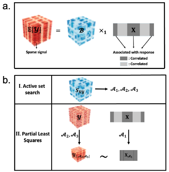
Figure 1: SHOPS overview. a. Problem formulation of the SHOPS model. SHOPS considers cases where the covariates/predictors in $X$ are highly correlated, and only a relatively small subset of the these associates with the mean tensor $\mathbb{E}[\mathcal{Y}]$. This sparsity is captured by sparse first mode of the coefficient tensor $\mathcal{B}$, where darker colors represent higher coefficient magnitudes. In addition, vast majority of the second and third mode entries of the mean tensor $\mathbb{E}[\mathcal{Y}]$ are zeros, as represented by the sparsity of the second and third modes of the coefficient tensor $\mathcal{B}$. SHOPS can simultaneously select important variables (darker shades in $X$) and detect mean tensor entries due to pure noise, while performing dimensionality reduction for the highly correlated variables. b. Summary of the SHOPS algorithm. SHOPS first identifies active sets $\mathcal{A}_{!}$, $\mathcal{A}_{2}$, $\mathcal{A}_{3}$ with an active set finding algorithm that employs soft-thresholding and hard-thresholding (Step I). Then, it fits ordinary tensor PLS onto reduced $\mathcal{Y}$ and $X$ to estimate non-zero entries of the coefficient tensor $\mathcal{B}$ (Step II).

We start out this section by formally defining the Sparse Higher Order Partial least Squares (SHOPS) model and present the specific algorithm for estimating the SHOPS model parameters in the next section. The SHOPS model for $\mathcal{Y}\in\mathbb{R}^{n\times d_{2}\times d_{3}}$ and $X\in\mathbb{R}^{n\times p}$ is

$$\mathcal{Y} =\mathcal{B}\times_{1}X+\sigma_{2}\mathcal{F}$$

$$=\mathcal{B}_{W}\times_{1}XW+\sigma_{2}\mathcal{F},$$ (1)

where for the covariance tensor $\Sigma_{X\mathcal{Y}}=\mathbb{E}[\mathcal{Y}\times_{1}X^{T}/n]$ and, for the active, i.e., non-zero, sets $\mathcal{A}_{1}^{*}\subset[p],\mathcal{A}_{2}^{*}\subset[d_{2}],\mathcal{A}_{3}^{*}\subset[d_{3}]$, the first, second, and third modes of $\Sigma_{X\mathcal{Y}}$ have only $\mathcal{A}_{1}^{*},\mathcal{A}_{2}^{*},\mathcal{A}_{3}^{*}$, entries non-zero, respectively. For example, for $i\in\mathcal{A}_{1}^{*C}$, we have the $i$th first mode slice as $\Sigma_{X\mathcal{Y}[i,\,,\,]}=\bm{0}\in\mathbb{R}^{d_{2}\times d_{3}}$. We further note that the data related to the active entries ($\mathcal{A}_{1}^{*},\mathcal{A}_{2}^{*},\mathcal{A}_{3}^{*}$) follow ordinary tensor PLS described in Section 2.2. Specifically, for the $k$th column vector of $W$, $\bm{w}_{k}$, and $W_{k}=(\bm{w}_{1},\cdots,\bm{w}_{k})$, the active entries of $\bm{w}_{k}$, defined as $\bm{w}_{k\mathcal{A}_{1}^{*}}$ is the first loading solution of $\max\limits_{\bm{s}_{1},\bm{s}_{2},\bm{s}_{3}}{\left(\left\lVert\Sigma_{X_{\mathcal{A}_{1}^{*}}\mathcal{Y}_{[\,,\mathcal{A}_{2}^{*},\mathcal{A}_{3}^{*}]}}\times_{1}\bm{s}_{1}\times_{2}\bm{s}_{2}\times_{3}\bm{s}_{3}\right\rVert_{F}^{2}\right)}$, satisfying $\bm{s}_{1}^{T}\Sigma_{X_{\mathcal{A}_{1}^{*}}X_{\mathcal{A}_{1}^{*}}}W_{k-1\mathcal{A}_{1}^{*}}=\bm{0}$ and $\bm{s}_{1}^{T}(I_{q_{1}}-W_{k-1\mathcal{A}_{1}^{*}}W^{+}_{k-1\mathcal{A}_{1}^{*}})\bm{s}_{1}=1$ with $\bm{s}_{1}\in\mathbb{R}^{q_{1}},\bm{s}_{2}\in\mathbb{S}^{q_{2}-1},\bm{s}_{3}\in\mathbb{S}^{q_{3}-1}$, where $q_{1},q_{2},q_{3}$ denote the cardinality of the active sets $\mathcal{A}_{1}^{*},\mathcal{A}_{2}^{*},\mathcal{A}_{3}^{*}$, respectively. Moreover, we assume that the inactive entries $\bm{w}_{k\mathcal{A}_{1}^{*C}}=0$, and hence $W_{\mathcal{A}_{1}^{*C}}=0$, where an active (or inactive) set subscript of $W$ refers to the extraction of only the active (or inactive) rows of the matrix and $\mathcal{Y}_{[\,,\mathcal{A}_{2}^{*},\mathcal{A}_{3}^{*}]}$ refers to extraction of active (or inactive) second and third mode entries of the tensor $\mathcal{Y}$. Then, given $W$, we have

$$\mathcal{B}=\Sigma_{X\mathcal{Y}}\times_{1}W(W^{T}\Sigma_{XX}W)^{-1}W^{T}.$$

Consequently, by the zero and non-zero patterns of $\Sigma_{X\mathcal{Y}}$ and $W$, the active set entries of $\mathcal{B}$, denoted as $\mathcal{B}_{\mathcal{A}_{1}^{*}\mathcal{A}_{2}^{*}\mathcal{A}_{3}^{*}}\in\mathbb{R}^{q_{1}\times q_{2}\times q_{3}}$, can be expressed as

$$\mathcal{B}_{\mathcal{A}_{1}^{*}\mathcal{A}_{2}^{*}\mathcal{A}_{3}^{*}}=\Sigma_{X_{\mathcal{A}_{1}^{*}}\mathcal{Y}_{[\,,\mathcal{A}_{2}^{*},\mathcal{A}_{3}^{*}]}}\times_{1}W_{\mathcal{A}_{1}^{*}}(W_{\mathcal{A}_{1}^{*}}^{T}\Sigma_{X_{\mathcal{A}_{1}^{*}}X_{\mathcal{A}_{1}^{*}}}W_{\mathcal{A}_{1}^{*}})^{-1}W_{\mathcal{A}_{1}^{*}}^{T},$$

which coincides with the ordinary tensor PLS estimator investigated in Section 2. Here, we use $X_{\mathcal{A}_{1}}$ as $\mathcal{A}_{1}$ columns of $X$ for an active set $\mathcal{A}_{1}$, while $W_{\mathcal{A}_{1}}$ refers to the extraction of ${\mathcal{A}_{1}}$ rows of $W$. In what follows, the tensors with the three active sets in the subscript, e.g., $\mathcal{B}_{\mathcal{A}_{1}\mathcal{A}_{2}\mathcal{A}_{3}}$, refer to the extraction of active (or inactive) first, second, and third mode entries of the original tensor. In contrast, we have the entire inactive set entries as $\mathcal{B}_{\mathcal{A}_{1}^{*C}\mathcal{A}_{2}^{*C}\mathcal{A}_{3}^{*C}}=\bm{0}\in\mathbb{R}^{(p-q_{1})\times(d_{2}-q_{2})\times(d_{3}-q_{3})}$. Hence, for this model, we first employ an active set finding algorithm that yields $\hat{\mathcal{A}}_{m}$ for each $m=1,2,3$ and identifies $\mathcal{A}^{*}_{m}$ with high probability. Subsequently, we employ the ordinary PLS onto only active sets of the data.

3.2 Implementation of the SHOPS model and the corresponding algorithms

The main SHOPS algorithm estimates the active sets $\mathcal{A}_{1}^{*},\mathcal{A}_{2}^{*},\mathcal{A}_{3}^{*}$ and then implements the tensor partial least squares regression algorithm described in Section 2.2 (Fig. 1b). The specific steps of the algorithm are presented in Algorithm 2.

Algorithm 2 Sparse higher order Partial Least Squares

Initialize $\hat{\mathcal{B}}_{SHOPS}=\bm{0}\in\mathbb{R}^{p\times d_{2}\times d_{3}}$.

1. Obtain non-zero active sets $\mathcal{A}_{1}$,$\mathcal{A}_{2}$,$\mathcal{A}_{3}$ by Algorithm 3.

2. Fit tensor PLS $\mathcal{Y}_{[\,,\mathcal{A}_{2},\mathcal{A}_{3}]}\sim X_{\mathcal{A}_{1}}$ with $K$ latent components by Algorithm 1 and obtain $\tilde{\mathcal{B}}\in\mathbb{R}^{|\mathcal{A}_{1}|\times|\mathcal{A}_{2}|\times|\mathcal{A}_{3}|}$.

3. Update $\hat{B}_{SHOPS}$ by the coefficient tensor $\tilde{\mathcal{B}}$ from step 2 through non-zero entries $\mathcal{A}_{1},\mathcal{A}_{2},\mathcal{A}_{3}$.

Return $\hat{\mathcal{B}}_{SHOPS}$

This algorithm yields the following coefficient tensor estimator

$$\hat{\mathcal{B}}_{SHOPS} =S_{X\mathcal{Y}}\times_{1}\hat{W}(\hat{W}^{T}S_{XX}\hat{W})^{-1}\hat{W}^{T}\times_{2}D_{\hat{\mathcal{A}}_{2}}\times_{3}D_{\hat{\mathcal{A}}_{3}}$$

$$=S_{X\mathcal{Y}}\times_{1}D_{\hat{\mathcal{A}}_{1}}\hat{W}(\hat{W}^{T}D_{\hat{\mathcal{A}}_{1}}S_{XX}D_{\hat{\mathcal{A}}_{1}}\hat{W})^{-1}\hat{W}^{T}D_{\hat{\mathcal{A}}_{1}}\times_{2}D_{\hat{\mathcal{A}}_{2}}\times_{3}D_{\hat{\mathcal{A}}_{3}},$$

where $D_{\mathcal{A}_{m}}=\mbox{diag}(\bm{1}_{\mathcal{A}_{m}})\in\mathbb{R}^{d_{m}\times d_{m}}$ for an active set $\mathcal{A}_{m}$, $m=1,2,3$. We further note that the estimated active entries of the estimator $\hat{\mathcal{B}}_{SHOPS}$ can be represented as

$$\hat{\mathcal{B}}_{SHOPS\hat{\mathcal{A}}_{1},\hat{\mathcal{A}}_{2},\hat{\mathcal{A}}_{3}}=S_{X_{\hat{\mathcal{A}}_{1}}\mathcal{Y}_{[\,,\hat{\mathcal{A}}_{2},\hat{\mathcal{A}}_{3}]}}\times_{1}W_{\hat{\mathcal{A}}_{1}}(W_{\hat{\mathcal{A}}_{1}}^{T}S_{X_{\hat{\mathcal{A}}_{1}}X_{\hat{\mathcal{A}}_{1}}}W_{\hat{\mathcal{A}}_{1}})^{-1}W_{\hat{\mathcal{A}}_{1}}^{T},$$

while the inactive ones are all zero.

For the active set finding step in the SHOPS main algorithm (step # 1 in Algorithm  2), we suggest a two-step thresholding scheme to find the non-zero entries of the covariance tensor $\Sigma_{X\mathcal{Y}}$. This algorithm operates by first soft-thresholding the sample coefficient tensor entry-wise and then hard-thresholding the loading vectors of the soft-thresholded tensor. A similar two-step thresholding algorithm was also employed in [26] for matrix Sparse Principal Component Analysis (SPCA). While the main analysis object is the covariate covariance matrix $\Sigma_{XX}$ in SPCA, our algorithm’s main object is the covariance tensor $\Sigma_{X\mathcal{Y}}$. A sample splitting procedure is also employed within the algorithm. The main benefit of the sample splitting is the decoupling of the dimension reduction (HOOI) and the selection of active sets (hard-thresholding) [27, 26]. Since the two randomly selected samples $\Omega_{1}\subset[n]$ and $\Omega_{2}\subset[n]$ are independent, given the first sample $\Omega_{1}$, we can regard the low-dimensional loadings, e.g., $\hat{\bm{u}}_{1r},\hat{\bm{u}}_{2r},\hat{\bm{u}}_{3r}$, as deterministic for the purposes of hard-thresholding.

Algorithm 3 Active set finding algorithm

$\Omega_{1}$: $n_{1}$ random samples from $[n]$, $\Omega_{2}$: $n_{2}$ samples $[n]/\Omega_{1}$, covariance tensors $S_{X\mathcal{Y}}=\mathcal{Y}[\Omega_{1},\,,\,]\times_{1}X[\Omega_{1},\,]^{T}/n_{1}$, $S_{X\mathcal{Y}}^{\prime}=\mathcal{Y}[\Omega_{2},\,,\,]\times_{1}X[\Omega_{2},\,]^{T}/n_{2}$, with $n_{1}=n_{2}=n/2$.

1. Compute the soft-thresholded covariance tensor $\eta(S_{X\mathcal{Y}})$ :

$$\eta(S_{X\mathcal{Y}})_{ijk}=\begin{cases}(S_{X\mathcal{Y}})_{ijk}-\frac{\tau}{\sqrt{n_{1}}}\mbox{ if }(S_{X\mathcal{Y}})_{ijk}\geq\frac{\tau}{\sqrt{n_{1}}}\\ 0\qquad\qquad\qquad\mbox{ if }|(S_{X\mathcal{Y}})_{ijk}|<\frac{\tau}{\sqrt{n_{1}}}\\ (S_{X\mathcal{Y}})_{ijk}+\frac{\tau}{\sqrt{n_{1}}}\mbox{ if }(S_{X\mathcal{Y}})_{ijk}\leq-\frac{\tau}{\sqrt{n_{1}}}.\end{cases}$$

2. Let $\hat{\tilde{\bm{u}}}_{1r}$, $\hat{\bm{u}}_{2r}$, $\hat{\bm{u}}_{3r}$ be ($r$th rank) loadings of $\eta(S_{X\mathcal{Y}})$ obtained from tensor power iteration. $\triangleright$ each rank 1 approximation obtained from HOOI

Return active sets $\mathcal{A}_{1}=\{i\in[p]:\exists r\mbox{ s.t. }|(S_{X\mathcal{Y}}^{\prime}\times_{2}\hat{\bm{u}}_{2r}^{T}\times_{3}\hat{\bm{u}}_{3r}^{T})_{i}|\geq T_{1r}\}$, $\mathcal{A}_{2}=\{i\in[d_{2}]:\exists r\mbox{ s.t. }|(S_{X\mathcal{Y}}^{\prime}\times_{1}\hat{\tilde{\bm{u}}}_{1r}^{T}\times_{3}\hat{\bm{u}}_{3r}^{T})_{i}|\geq T_{2r}\}$, $\mathcal{A}_{3}=\{i\in[d_{3}]:\exists r\mbox{ s.t. }|(S_{X\mathcal{Y}}^{\prime}\times_{2}\hat{\bm{u}}_{2r}^{T}\times_{3}\hat{\bm{u}}_{3r}^{T})_{i}|\geq T_{3r}\}$.

We employ a hypothesis testing framework for setting the thresholding parameters $\tau$, $T_{1r}$, $T_{2r}$, $T_{3r}$ in practice. This results in choosing only one parameter $\nu$ for $\tau$, $T_{1r}$, $T_{2r}$, $T_{3r}$, which corresponds to the standard deviation step-size in the testing procedure details of which are discussed in Section 3.4. In the next section, we investigate the probabilistic performance of the active set finding algorithm and derive the asymptotic results of the sparse higher order partial least squares estimator.

3.3 Asymptotic results for sparse higher order partial least squares

In this section, we derive the asymptotic properties of the SHOPS estimator when the dimensions of the entire tensor coefficient ($p$, $d_{2}$, $d_{3}$) grow possibly faster than the sample size $n$. We first assume that, as in the ordinary tensor partial least squares, Assumptions 1 and 2 hold. For Assumption 1, we have $X=V\Gamma^{T}+\sigma_{1}E$ for $\Gamma=(\bm{\gamma}_{1},\cdots,\bm{\gamma}_{m})\in\mathbb{R}^{p\times m}$, $V=(\bm{v}_{1}\cdots,\bm{v}_{m})\in\mathbb{R}^{n\times m}$, $E=(\bm{e}_{1}^{T}\cdots,\bm{e}_{n}^{T})^{T}\in\mathbb{R}^{n\times p}$. We denote $\alpha\coloneqq\left\lVert\Gamma\right\rVert_{2}$ in the following theorems.

Once we impose Assumption 2, for $\Sigma_{X\mathcal{Y}}=\Sigma_{XX}\mathcal{B}=\tilde{\vartheta}(\tilde{\bm{u}}_{1}\circ\bm{u}_{2}\circ\bm{u}_{3})$, we have $\left\lVert\tilde{\bm{u}}_{1}\right\rVert_{0}\leq q_{1}$, $\left\lVert\bm{u}_{2}\right\rVert_{0}\leq q_{2}$, $\left\lVert\bm{u}_{3}\right\rVert_{0}\leq q_{3}$, where $\tilde{\bm{u}}_{1}=\Sigma_{XX}\bm{u}_{1}/\left\lVert\Sigma_{XX}\bm{u}_{1}\right\rVert_{2}$ and $\tilde{\vartheta}=\left\lVert\Sigma_{XX}\bm{u}_{1}\right\rVert_{2}$, and $\left\lVert\cdot\right\rVert_{0}$ is defined as the number of zeros of a vector. This assumption on the coefficient tensor is employed for establishing theoretical characteristics of the SHOPS estimator. However, our empirical results from the simulation experiments reveal that SHOPS can be applied for general rank $R$ in various settings, especially when the covariance tensor is orthogonally decomposable, i.e., when we have $\Sigma_{X\mathcal{Y}}=\sum_{r=1}^{R}\tilde{\vartheta_{r}}(\tilde{\bm{u}}_{1r}\circ\bm{u}_{2r}\circ\bm{u}_{3r})$ with $\tilde{\bm{u}}_{1r}^{T}\tilde{\bm{u}}_{1s}=0$, $\bm{u}_{2r}^{T}\bm{u}_{2s}=0$, and $\bm{u}_{3r}^{T}\bm{u}_{3s}=0$ for different $r,s\in[R]$.

We further impose the reduced form of the [12] condition similar to Condition 1, which is a standard condition imposed in the PLS literature.

Condition 2

There exist $K$ eigenvectors $\bm{\tilde{\gamma}}_{k}$ $(k=1,\cdots,K)$ of $\Sigma_{XX}$ corresponding to different eigenvalues, such that for $\tilde{\bm{\alpha}}_{ij}=(\tilde{\alpha}_{ij1},\cdots,\tilde{\alpha}_{ijK})$, $\tilde{\Gamma}_{K}=(\bm{\tilde{\gamma}}_{1},\cdots,\bm{\tilde{\gamma}}_{K})$ and for $i\in\mathcal{A}_{2}^{*},j\in\mathcal{A}_{3}^{*}$, the following holds

$$\Sigma_{X\mathcal{Y}[\mathcal{A}_{1}^{*},i,j]}=\tilde{\Gamma}_{K\mathcal{A}_{1}^{*}}\tilde{\bm{\alpha}}_{ij},$$

where $\tilde{\alpha}_{ijk}$ are non-zero scalars, and $\Sigma_{X\mathcal{Y}[\mathcal{A}_{1}^{*},i,j]}\in\mathbb{R}^{q_{1}}$ is the $(i,j)$th first mode fiber of $\Sigma_{X\mathcal{Y}[\mathcal{A}_{1}^{*},\,,\,]}\in\mathbb{R}^{q_{1}\times d_{2}\times d_{3}}$ and $\tilde{\Gamma}_{K\mathcal{A}_{1}^{*}}$ is the $\mathcal{A}_{1}^{*}$ rows of $\tilde{\Gamma}_{K}$.

While we directly impose sparsity on the first mode of the covariance tensor in the model (3.1) and assume by Condition 2 that the active first mode entries of the covariance tensor are constructed by $K$ eigenvectors $\tilde{\Gamma}_{K}$ of the covariance matrix $\Sigma_{XX}$, we can also indirectly impose the sparsity on the first mode of the covariance tensor along with a stricter condition than Condition 2. This condition, as outlined in Condition 3 below, imposes row-wise sparsity on the $K$ eigenvectors of $\Sigma_{XX}$ as follows.

Condition 3

There exist $K$ eigenvectors $\bm{\tilde{\gamma}}_{k}$ $(k=1,\cdots,K)$ of $\Sigma_{XX}$ corresponding to different eigenvalues, such that for $\tilde{\bm{\alpha}}_{ij}=(\tilde{\alpha}_{ij1},\cdots,\tilde{\alpha}_{ijK})$, $\tilde{\Gamma}_{K}=(\bm{\tilde{\gamma}}_{1},\cdots,\bm{\tilde{\gamma}}_{K})$ and for $i\in\mathcal{A}_{2}^{*},j\in\mathcal{A}_{3}^{*}$, the following holds

$$\Sigma_{X\mathcal{Y}[\,,i,j]}=\tilde{\Gamma}_{K}\tilde{\bm{\alpha}}_{ij},\quad\tilde{\Gamma}_{K\mathcal{A}_{1}^{*C}}=\bm{0}\in\mathbb{R}^{(p-q_{1})\times K},$$

where $\tilde{\alpha}_{ijk}$ are non-zero scalars, and $\Sigma_{X\mathcal{Y}[\,,i,j]}\in\mathbb{R}^{p}$ is the $(i,j)$th first mode fiber of the covariance tensor $\Sigma_{X\mathcal{Y}}\in\mathbb{R}^{p\times d_{2}\times d_{3}}$ and $\tilde{\Gamma}_{K\mathcal{A}_{1}^{*C}}$ is the $\mathcal{A}_{1}^{*C}$ rows of $\tilde{\Gamma}_{K}$.

Without loss of generality, if we assume that the first $q_{1}$ entries of $[p]$ is $\mathcal{A}_{1}^{*}$, Condition 3 can be stated as

$$\Sigma_{X\mathcal{Y}[\,,i,j]}=\begin{bmatrix}\tilde{\Gamma}_{K\mathcal{A}_{1}^{*}}\\ \bm{0}\end{bmatrix}\tilde{\bm{\alpha}}_{ij}.$$

Based on the connection between PLS and Envelope model established in [28], SHOPS with Condition 3 imposes similar sparsity structure on the first mode of $\mathcal{B}$ as the matrix Envelope-SPLS model [29]. Specifically, the sparsity is applied to the relevant basis matrix, denoted by $\tilde{\Gamma}_{K}$, which encompasses the association between $X$ and $\mathcal{Y}$.

For the consistency proof of SHOPS, we first argue that the active set finding algorithm correctly finds the true non-zero entries $\mathcal{A}_{1}^{*},\mathcal{A}_{2}^{*},\mathcal{A}_{3}^{*}$ with high probability, and prove the consistency of $\hat{\mathcal{B}}_{SHOPS}$ given true active sets $\mathcal{A}_{1}^{*},\mathcal{A}_{2}^{*},\mathcal{A}_{3}^{*}$. Then, by combining the two results, we obtain the consistency of $\hat{\mathcal{B}}_{SHOPS}$.

We argue that the Active set finding algorithm identifies true non-zero entries with high probability with the following three steps: Step 1: Soft-thresholded covariance tensor $\eta(S_{X\mathcal{Y}})$ is close to the true covariance tensor $\Sigma_{X\mathcal{Y}}$ with high probability with a rate of $O_{p}(\sqrt{q_{1}q_{2}q_{3}\log{(pd_{2}d_{3})}/n})$. Step 2: The loading vector estimates of the soft-thresholded covariance tensor $\eta(S_{X\mathcal{Y}})$ are close enough to the true loading vectors of the population covariance tensor with rate $O_{p}(\sqrt{q_{1}q_{2}q_{3}\log{(pd_{2}d_{3})}/n})$. Step 3: The hard-thresholding step correctly identifies the non-zero entries with high probability. Lemma LABEL:supp-lem:soft and Lemma LABEL:supp-lem:dist in the Supplementary Materials Section LABEL:supp-sectionS:proofs prove Step 1 and Step 2, respectively. With these results, we are able to establish that the hard-thresholding step of active set finding algorithm correctly finds the true active sets with high probability as the sample size grows faster than the number of non-zero entries.

Theorem 2

Assume that Assumption 1, Assumption 2, Condition 2 (or Condition 3), and the assumptions for Lemma LABEL:supp-lem:soft hold. Further assume that there exist $\lambda_{1}$, $\lambda_{2}$, $\lambda_{3}>0$ satisfying $\vartheta|\phi_{i}+\sigma_{1}^{2}u_{1i}|\geq\frac{\tilde{\vartheta}\lambda_{1}}{\sqrt{q_{1}q_{2}q_{3}}}$, $|u_{2j}|\geq\frac{\lambda_{2}}{\sqrt{q_{1}q_{2}q_{3}}}$, $|u_{3k}|\geq\frac{\lambda_{3}}{\sqrt{q_{1}q_{2}q_{3}}}$ for all $i\in\mathcal{A}_{1}^{*}$, $j\in\mathcal{A}_{2}^{*}$, $k\in\mathcal{A}_{3}^{*}$, where $\phi_{i}$ is $i$th entry of $\Gamma\Gamma^{T}\bm{u}_{1}$, $u_{1i}$ denotes $i$th entry of $\bm{u}_{1}$, $u_{2j}$ denotes $j$th entry of $\bm{u}_{2}$, $u_{3k}$ denotes $k$th entry of $\bm{u}_{3}$. Lastly, assume that there exist a large global constant $C_{0}$ satisfying $n>C_{0}((\alpha+\sigma_{1})^{4}\vee 1)(\vartheta+\sigma_{2})^{2}/(\tilde{\vartheta}^{2}\lambda_{\mbox{min}}^{2})q_{1}q_{2}q_{3}\log{(pd_{2}d_{3})}$, where $\lambda_{\mbox{min}}=\lambda_{1}\wedge\lambda_{2}\wedge\lambda_{3}$. With the covariance tensor thresholding algorithm, employing $\tau=C_{1}(\sigma_{1}\vartheta+\sigma_{2})(\alpha+\sigma_{1})\sqrt{\log{pd_{2}d_{3}}}$ for a constant $C_{1}$ and $T_{k}=\tilde{\vartheta}\lambda_{k}/(2\sqrt{q_{1}q_{2}q_{3}})$ for $k=1,2,3$, we have

$$\mathbb{P}(\hat{\mathcal{A}}=\mathcal{A}^{*})\geq 1-o(1),$$

where $\mathcal{A}^{*}=\mathcal{A}_{1}^{*}\times\mathcal{A}_{2}^{*}\times\mathcal{A}_{3}^{*}$, $\hat{\mathcal{A}}=\hat{\mathcal{A}}_{1}\times\hat{\mathcal{A}}_{2}\times\hat{\mathcal{A}}_{3}$.

Theorem 2 implies that as we have $q_{1}q_{2}q_{3}\log{(pd_{2}d_{3})}/n\rightarrow 0$, we are able to find the true active set $\mathcal{A}^{*}$ with probability tending to 1. Here, the $\log$ term represents the difficulty level of finding unknown non-zero entries, while the term $q_{1}q_{2}q_{3}/n$ is the rate related to the convergence of sample covariance tensor to the true counter part. Next, we suggest and prove that the NIPALS tensor SHOPS estimator $\hat{\mathcal{B}}_{SHOPS}$ achieves $\sqrt{n}$-consistency upto a logarithmic factor under the high-dimensional regime, i.e., $\left\lVert\hat{\mathcal{B}}_{SHOPS}-\mathcal{B}\right\rVert_{F}\leq O_{p}\left(\sqrt{q_{1}q_{2}q_{3}\log{(pd_{2}d_{3})/n}}\right)$.

Theorem 3

Under Assumption 1, Assumption 2, Condition 2 (or Condition 3) and the assumptions for Theorem 2, and with the thresholding parameters given in Lemma LABEL:supp-lem:soft and Lemma LABEL:supp-lem:dist, we have

$$\mbox{(a) if }q_{1}q_{2}q_{3}\log{(pd_{2}d_{3})}/n\rightarrow 0,\mbox{ then }\mathbb{P}(\hat{\mathcal{A}}=\mathcal{A}^{*})\rightarrow 1\mbox{ and }\left\lVert\hat{\mathcal{B}}_{SHOPS}-\mathcal{B}\right\rVert_{F}\stackrel{{\scriptstyle p}}{{\rightarrow}}0.$$

$$\mbox{(b) if }\mathbb{P}(\hat{\mathcal{A}}=\mathcal{A}^{*})\rightarrow 1\mbox{ and }\left\lVert\hat{\mathcal{B}}_{SHOPS}-\mathcal{B}\right\rVert_{F}\rightarrow 0\mbox{ in probability},\mbox{ then }q_{1}q_{2}q_{3}/n\rightarrow 0,$$

where the $\hat{\mathcal{B}}_{SHOPS}$ is obtained from the SHOPS algorithm.

Theorem 3 demonstrates the clear advantage of using SHOPS model over using ordinary tensor PLS. As emphasized in Theorem 1, the consistency of tensor PLS cannot be guaranteed when $pd_{2}d_{3}\gg n$. In contrast, SHOPS model can still identify the correct non-zero sets and guarantee the convergence of the coefficient estimate even when $pd_{2}d_{3}\gg n$, as long as $q_{1}q_{2}q_{3}\lesssim n$ up to logarithmic factor. The bound $\left\lVert\hat{\mathcal{B}}_{SHOPS}-\mathcal{B}\right\rVert_{F}\leq O_{p}\left(\sqrt{q_{1}q_{2}q_{3}\log{(pd_{2}d_{3})}/n}\right)$ in the proof of the Theorem 3 matches the ones established in [18, 20] for the ordinary sparse tensor regression without the PLS set up. When both $d_{2}$, $d_{3}=1$, so that the problem becomes univariate sparse least squares, we obtain the bound $O_{p}\left(\sqrt{q_{1}\log{p}/n}\right)$, which is shown to be minimax optimal for the ordinary (non-PLS) sparse vector regression with $\left\lVert\beta\right\rVert_{0}\leq q_{1}$ [30].

In scientific applications such as the single cell 3D genome organization with scHi-C and single cell DNA methylation data, we expect methylation of a small number of genomic regions ($q_{1}$) to significantly affect the long-range physical contact between a small number of genomic locus pairs ($q_{2}$, $q_{3}$). Therefore, we can reasonably assume sparsity on the covariance structure $\Sigma_{X\mathcal{Y}}$ and expect to obtain markedly better accuracy of the coefficient tensor estimator.

3.4 Practical considerations for selecting the thresholding parameter and the number of components

While there are four parameters ($\tau$, $T_{1r}$, $T_{1r}$, $T_{1r}$) to set for the thresholding operations in Algorithm 3, we need to only tune one parameter $\nu$, which corresponds to the step-size of the standard deviation for all the thresholding tasks. This is motivated by the following hypothesis testing based argument.

3.4.1 Choice of the soft-thresholding parameter $\tau$

Consider the null hypothesis that $\mathbb{E}({S_{X\mathcal{Y}}}_{ijk})=0$, and the standard deviation $\sigma({S_{X\mathcal{Y}}}_{ijk})=\sigma_{2}\sqrt{(\left\lVert\bm{\gamma}^{i}\right\rVert_{2}^{2}+\sigma_{1}^{2})}/\sqrt{n_{1}}$ obtained from the SHOPS model (3.1), where $\bm{\gamma}^{i}\in\mathbb{R}^{m}$ is $i$th row of the matrix $\Gamma=(\bm{\gamma}_{1},\cdots,\bm{\gamma}_{m})$ in Assumption 1. We “reject” the null if $|{S_{X\mathcal{Y}}}_{ijk}|>\nu\sigma({S_{X\mathcal{Y}}}_{ijk})$ for some $\nu\geq 0$.

Next, we discuss how to estimate $\sigma_{2}$ and $\sqrt{(\left\lVert\bm{\gamma}^{i}\right\rVert_{2}^{2}+\sigma_{1}^{2})}$ in the expression $\sigma({S_{X\mathcal{Y}}}_{ijk})$. For the $i$th covariate, we have $\sqrt{{(\Sigma_{XX})}_{ii}}=\sqrt{(\left\lVert\bm{\gamma}^{i}\right\rVert_{2}^{2}+\sigma_{1}^{2})}$ by Assumption 1. Therefore, we estimate the term $\sqrt{(\left\lVert\bm{\gamma}^{i}\right\rVert_{2}^{2}+\sigma_{1}^{2})}$ as the standard deviation of $X_{i}$, e.g., $\mbox{MAD}(X_{i})/\Phi^{-1}(3/4)$ or $\mbox{s.d.}(X_{i})$, where $\mbox{s.d.}(\cdot)$ refers to standard deviation, $\mbox{MAD}(\cdot)$ is the median absolute deviation and $\Phi(\cdot)$ is the c.d.f of standard normal distribution. As for the estimate of $\sigma_{2}$ in the model (3.1), we suggest using the sample standard devation estimate or $\mbox{MAD}(\mathcal{Y})/\Phi^{-1}(3/4)$ or $\mbox{s.d.}(\mathcal{Y})$. As a result, we recommend to use the estimate

$$\hat{\sigma}({S_{X\mathcal{Y}}}_{ijk})=\frac{1}{\sqrt{n_{1}}}\frac{\mbox{MAD}(X_{i})}{\Phi^{-1}(3/4)}\frac{\mbox{MAD}(\mathcal{Y})}{\Phi^{-1}(3/4)}\quad\left(\mbox{or }\frac{1}{\sqrt{n_{1}}}\mbox{s.d.}(X_{i})\mbox{s.d.}(\mathcal{Y})\right),$$

i.e., set the thresholding parameter $\tau\equiv\nu\hat{\sigma}({S_{X\mathcal{Y}}}_{ijk})$, and perform soft-thresholding based on the criterion $|{S_{X\mathcal{Y}}}_{ijk}|>\tau/\sqrt{n_{1}}$.

3.4.2 Choice of the hard-thresholding parameters $T_{1r}$, $T_{2r}$, $T_{3r}$

For each $r\in[R]$, and for the first mode, we have $S_{X\mathcal{Y}}^{\prime}\times_{2}\hat{\bm{u}}_{2r}^{T}\times_{3}\hat{\bm{u}}_{3r}^{T}=\tilde{\bm{u}}_{1r}+\epsilon_{1r}$, where the true first loading $\tilde{\bm{u}}_{1r}=\Sigma_{XX}\bm{u}_{1r}/\left\lVert\Sigma_{XX}\bm{u}_{1r}\right\rVert_{2}$. Under the null hypothesis that $i$th entry of $\tilde{\bm{u}}_{1r}$ is zero, we have $\left(S_{X\mathcal{Y}}^{\prime}\times_{2}\hat{\bm{u}}_{2r}^{T}\times_{3}\hat{\bm{u}}_{3r}^{T}\right)_{i}=\epsilon_{1i}$. Hence, we reject the null hypothesis if $|\left(S_{X\mathcal{Y}}^{\prime}\times_{2}\hat{\bm{u}}_{2r}^{T}\times_{3}\hat{\bm{u}}_{3r}^{T}\right)_{i}|>\nu\sigma_{\epsilon_{1r}}$. Here, we suggest to estimate the standard deviation of $\epsilon_{1r}$, $\sigma_{\epsilon_{1r}}$ as

$$\hat{\sigma}_{\epsilon_{1r}}=\frac{\mbox{MAD}(S_{X\mathcal{Y}}^{\prime}\times_{2}\hat{\bm{u}}_{2r}^{T}\times_{3}\hat{\bm{u}}_{3r}^{T})}{\Phi^{-1}(3/4)}\quad\left(\mbox{or }\mbox{s.d.}(S_{X\mathcal{Y}}^{\prime}\times_{2}\hat{\bm{u}}_{2r}^{T}\times_{3}\hat{\bm{u}}_{3r}^{T})\right).$$

Likewise, for mode 2 and 3, we use

$$\hat{\sigma}_{\epsilon_{2r}} =\frac{\mbox{MAD}(S_{X\mathcal{Y}}^{\prime}\times_{1}\hat{\tilde{\bm{u}}}_{1r}^{T}\times_{3}\hat{\bm{u}}_{3r}^{T})}{\Phi^{-1}(3/4)}\quad\left(\mbox{or }\mbox{s.d.}(S_{X\mathcal{Y}}^{\prime}\times_{1}\hat{\tilde{\bm{u}}}_{1r}^{T}\times_{3}\hat{\bm{u}}_{3r}^{T}))\right),$$

$$\hat{\sigma}_{\epsilon_{3r}} =\frac{\mbox{MAD}(S_{X\mathcal{Y}}^{\prime}\times_{1}\hat{\tilde{\bm{u}}}_{1r}^{T}\times_{2}\hat{\bm{u}}_{2r}^{T})}{\Phi^{-1}(3/4)}\quad\left(\mbox{or }\mbox{s.d.}((S_{X\mathcal{Y}}^{\prime}\times_{1}\hat{\tilde{\bm{u}}}_{1r}^{T}\times_{2}\hat{\bm{u}}_{2r}^{T})))\right),$$

to plug in $(S_{X\mathcal{Y}}^{\prime}\times_{1}\hat{\tilde{\bm{u}}}_{1r}^{T}\times_{3}\hat{\bm{u}}_{3r}^{T})_{i}>\nu\sigma_{\epsilon_{2r}}$ and $(S_{X\mathcal{Y}}^{\prime}\times_{1}\hat{\tilde{\bm{u}}}_{1r}^{T}\times_{2}\hat{\bm{u}}_{2r}^{T})_{i}>\nu\sigma_{\epsilon_{3r}}$, respectively. Consequently, the hard-thresholding parameters are set as $T_{1r}=\nu\hat{\sigma}_{\epsilon_{1r}}$, $T_{2r}=\nu\hat{\sigma}_{\epsilon_{2r}}$, $T_{3r}=\nu\hat{\sigma}_{\epsilon_{3r}}$.

In practice, $\nu$ for both the soft- and hard-threholding is tuned by cross-validation (CV) along with the number of latent components $K$ of the SHOPS. When the explanatory variables are low dimensional (small $p$) and the sparsity on the first mode of the coefficient tensor $\mathcal{B}$ is not of interest, one can simply set $T_{1r}=0$ and perform CV by only varying the thresholding parameters of the second and third modes. Same strategy can be used for the second and third modes. When CV for choosing $\nu$ is not desirable/feasible (i.e., due to computational complexity), we suggest a Gaussian Mixture Model based approach to determine thresholding parameters in Supplementary Section LABEL:supp-GMM_thr.

3.4.3 Choice of number of latent components

Conditions 1 and 2 imply that the number of eigenvectors of $\Sigma_{XX}$ with distinct eigenvalues, denoted as $m$, cannot be smaller than the latent PLS directions $K$. Hence, $m$ is a natural upper bound when performing CV for $K$. We recommend performing eigen decomposition of $S_{XX}$ and choosing the estimate of $m$ as the elbow point of the eigenvalue scree plot. Similarly, for the power-iteration number $R$ in the active set finding algorithm, we perform SVD on all three unfolded $S_{X\mathcal{Y}}$ and take the minimum elbow point of the singular value plots as $R$.

4 Simulation studies

We next provide a wide range of simulation settings to empirically evaluate the properties of SHOPS and benchmark it against alternatives. The overall data generating schemes of these simulations were set as follows (Fig 2):

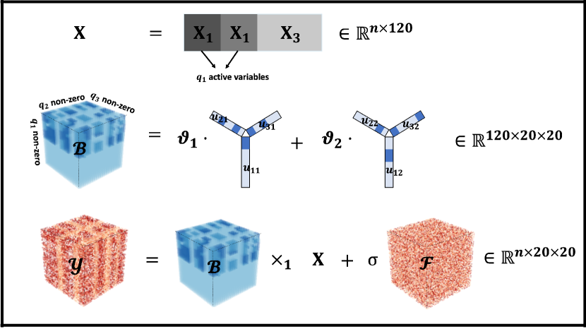
Figure 2: Overview of the data generating scheme in the simulations. First row: Covariate matrix $X$ consists of three sets of variables $X_{1}$, $X_{2}$, $X_{3}$, with high correlations among the variables within the same group. Second row: Generation of the true coefficient tensor $\mathcal{B}$, which has $q_{1}$, $q_{2}$, $q_{3}$ numbers of non-zero (active) entries for each mode. The structure of $\mathcal{B}$ indicates that the set of variables in $X_{3}$ are all inactive variables. Third row: Generation of the response tensor $\mathcal{Y}$ as an addition of mean tensor $\mathcal{B}\times_{1}X$ and the noise tensor $\mathcal{F}$. Lightest blue and red shades correspond to 0 entries in the tensor objects. For each tensor, lighter (blue or red) colored entries have smaller absolute values.

• Covariate matrix: $X=V\Gamma^{T}+\sigma_{1}E\in\mathbb{R}^{n\times 120}$, where $V=[\bm{v}_{1},\bm{v}_{2},\bm{v}_{3}]$, $\bm{v}_{k}\sim N(0,I_{n})$, $\Gamma=\alpha[\bm{\gamma}_{1},\bm{\gamma}_{2},\bm{\gamma}_{3}]$, $\tilde{\bm{\gamma}}_{1}=[\bm{1}^{T}_{\frac{q_{1}}{2}},\bm{0}^{T}_{\frac{q_{1}}{2}},\bm{0}^{T}_{120-q_{1}}]^{T}$,$\tilde{\bm{\gamma}}_{2}=[\bm{0}^{T}_{\frac{q_{1}}{2}},\bm{1}^{T}_{\frac{q_{1}}{2}},\bm{0}^{T}_{120-q_{1}}]^{T}$,$\tilde{\bm{\gamma}}_{3}=[\bm{0}^{T}_{\frac{q_{1}}{2}},\bm{0}^{T}_{\frac{q_{1}}{2}},\bm{1}^{T}_{120-q_{1}}]^{T}$, $E_{ij}\stackrel{{\scriptstyle i.i.d}}{{\sim}}N(0,1)$, where $\bm{\gamma}_{k}$ is euclidean norm normalized version of $\tilde{\bm{\gamma}}_{k}$. We set $\sigma_{1}=0.25$, and $\alpha=\sqrt{2}$ for all cases.

• Coefficient tensor: $\mathcal{B}=\sum_{r=1}^{2}{\vartheta_{r}(\bm{u}_{1r}\circ\bm{u}_{2r}\circ\bm{u}_{3r})}$, where $U_{1}=[\bm{u}_{11},\bm{u}_{12}]\in\mathbb{R}^{120\times 2}$ is a column-wise unit euclidean norm normalization of $\tilde{U}_{1}=\Gamma A$, where $A\in\mathbb{R}^{3\times 2}$ is a random column-wise orthonormal matrix such that the third row $A_{[3,\,]}=0$. For the second mode, $U_{2}=[\bm{u}_{21},\bm{u}_{22}]\in\mathbb{R}^{20\times 2}$ is generated as a random column-wise orthonormal matrix, and the number of non-zero rows are $q_{2}$. Here, $\bm{u}_{21}$ and $\bm{u}_{22}$ do not necessarily have the same non-zero patterns. Similarly, for the third mode, $U_{3}=[\bm{u}_{31},\bm{u}_{32}]\in\mathbb{R}^{20\times 2}$ is generated as a random column-wise orthonormal matrix, and the number of non-zero rows are set to $q_{3}$. Similarly, $\bm{u}_{31}$ and $\bm{u}_{32}$ do not necessarily have the same non-zero patterns. The signal size $\vartheta_{r}=\vartheta$ for $\forall r=1,2$.

• Response tensor: $\mathcal{Y}=\mathcal{B}\times_{1}X+\sigma_{2}\mathcal{F}\in\mathbb{R}^{n\times 20\times 20}$, where $F_{ij}\stackrel{{\scriptstyle i.i.d}}{{\sim}}N(0,1)$.

There are several important points to highlight in this simulation set-up. First is related to the simultaneous variable selection and dimension reduction task. While the covariance matrix of $X$, $\Sigma_{XX}=\Gamma\Gamma^{T}+\sigma_{1}^{2}I_{p}$ consists of three orthogonal directions $\bm{\gamma}_{1},\bm{\gamma}_{2},\bm{\gamma}_{2}$, we note that the first mode loading, i.e., $(\Sigma_{XX}\bm{u}_{1r})$, of the covariance tensor $\Sigma_{X\mathcal{Y}}=\mathcal{B}\times_{1}\Sigma_{XX}=\sum_{r=1}^{R}\vartheta_{r}(\Sigma_{XX}\bm{u}_{1r})\circ\bm{u}_{2r}\circ\bm{u}_{3r}$ is constructed only through $\bm{\gamma}_{1},\bm{\gamma}_{2}$. Specifically, the first loading of the covariance tensor can be summarized as $(\Sigma_{XX}\bm{u}_{1r})=(\Gamma\Gamma^{T}+\sigma_{1}^{2}I_{p})\Gamma A_{[\,,r]}=(\alpha^{2}+\sigma_{1}^{2})\Gamma A_{[\,,r]}$ by the fact that $\Gamma^{T}\Gamma=\alpha^{2}I_{3}$. Since we have $A_{[3,\,]}=0$, the third column of $\Gamma$, i.e., $\bm{\gamma}_{3}$, does not contribute to generating the first loading $(\Sigma_{XX}\bm{u}_{1r})$ of the covariance tensor. Therefore, for $X=[X_{1},X_{2},X_{3}]$ with $X_{1}\in\mathbb{R}^{n\times\frac{q_{1}}{2}}$, $X_{2}\in\mathbb{R}^{n\times\frac{q_{1}}{2}}$, $X_{3}\in\mathbb{R}^{n\times(120-q_{1})}$, where each column of $X_{k}$ is $\bm{v}_{k}$ plus random noise, the groups of variables $X_{1},X_{2}$ are related to the mean response tensor, while the last $120-q_{1}$ variables in $X_{3}$ do not contribute to the construction of the mean tensor. Hence, a successful dimension reduction method should be able to discriminate the signals coming from $X_{1},X_{2}$ and the false signal coming from $X_{3}$. In this scenario, non-PLS-based dimension reduction methods, including PCR or even Sparse PCR, are not expected to result in a coefficient estimator exhibiting less contribution of $X_{3}$ than $X_{1}$, $X_{2}$. This is because if we only take into account the space generated by $X$, all three directions $\bm{\gamma}_{1}$, $\bm{\gamma}_{2}$, and $\bm{\gamma}_{3}$ are contributing equivalently.

While PLS-type methods can leverage the fact that $X_{3}$ (or $\bm{v}_{3}$) is irrelevant to the effect of $X$ on $\mathcal{Y}$ when performing dimension reduction, PLS models that are not explicitly assuming sparsity on the latent directions do not result in variable selection, hindering the practical interpretability of results. In contrast, we expect that SHOPS can perform such dimension reduction and variable selection tasks simultaneously by estimating the latent directions $W$ of the covariance tensor $\Sigma_{X\mathcal{Y}}$ by incorporating sparsity.

This simulation set up further reveals that the true covariance tensor $\Sigma_{X\mathcal{Y}}$ has only $q_{2}$ and $q_{3}$ non-zero entries for the second and the third modes, respectively. Therefore, the true coefficient tensor $\mathcal{B}$ should also have $q_{2}$ and $q_{3}$ non-zeros in its second and third modes. We remark that a PLS based multivariate response model that only incorporates the sparsity on its first loading (variable selection) direction, such as SPLS in a matrix case, will still leave those in-active $d_{2}-q_{2}$ and $d_{3}-q_{3}$ entries as active. In contrast, since SHOPS takes into account such sparsity on the remaining loadings (second and third directions), it will threshold out (or denoise) the irrelevant components of the coefficient tensor $\mathcal{B}$ simultaneously with the dimension reduction and variable selection, which happens in the first loading.

In what follows, we evaluate how SHOPS performs for the tasks outlined in the simulation set up in comparison to other baseline tensor partial least squares models in two aspects: active set finding and consistency of the estimator.

4.1 Comparison of SHOPs with baseline sparse tensor decomposition methods in identifying active sets

Both the SHOPS algorithm and the theoretical results of SHOPS emphasize the importance of identifying true active sets $\mathcal{A}_{1}^{*},\mathcal{A}_{2}^{*},\mathcal{A}_{3}^{*}$ for the performance of the SHOPS model. In order to empirically validate the result of Theorem 2 that SHOPS correctly identifies active sets with high probability, we compared the performance of the active set finding algorithm of SHOPS against other baseline sparse tensor decomposition methods: Sparse Higher Order Singular Value Decomposition (HOSVD) and Sparse Higher Order Orthogonal Iteration (HOOI). Sparse HOSVD (SHOSVD) and Sparse HOOI (SHOOI) are sparse modifications of the Higher Order Singular Value Decomposition [31] and Higher Order Orthogonal Iteration algorithm [22], respectively. Both impose soft-thresholding on each of the Singular Value Decomposition (SVD) applied to unfolded (or matricized) tensors. Specifically, the sparse SVD is conducted following the algorithm introduced in [32]. Details on the specific algorithms for SHOOI and SHOSVD can be found in [33].

In order to evaluate the performances of the methods in a wide variety of settings, we varied the sample size as $n=200,400,600$, sparsity level $(\frac{q_{1}}{p}=\frac{q_{2}}{d_{2}}=\frac{q_{3}}{d_{3}})$ as $\mbox{sparsity}=0.25,0.4,0.7$, signal size as $\vartheta=0.25,0.5,1$, and the noise size as $\sigma_{2}=0.01,0.25,1$. Specifically, we considered a default setting $(n,\mbox{sparsity},\vartheta,\sigma_{2})=(600,0.5,1,0.25)$ and then varied one parameter at a time. For example, for the case where we varied the sparsity level in Fig 3b, we set $(n,\vartheta,\sigma_{2})=(600,1,0.25)$ and varied the sparsity level. For each set up, 40 simulated datasets were generated and results were averaged over these. The active set search performance is evaluated by the search error rate for each mode $M\in\{1,2,3\}$, defined as $(FNR_{M}+FPR_{M})/2$. Here, the false negative rate of $M$th mode is denoted as $FNR_{M}=\frac{|\mathcal{A}_{M}^{*}\cap\hat{\mathcal{A}}_{M}^{C}|}{|\mathcal{A}_{M}^{*}|}$, and the false positive rate of $M$th mode is denoted as $FPR_{M}=\frac{|\mathcal{A}_{M}^{*C}\cap\hat{\mathcal{A}}_{M}|}{|\mathcal{A}_{M}^{*C}|}$, where $\hat{\mathcal{A}}_{M}$ and $\hat{\mathcal{A}}_{M}^{C}$ denote the estimated active and inactive sets for mode $M$.

Fig. 3 summarizes the results across all the settings and suggests that as the sample size, sparsity level, and signal size increase, and as the noise level decreases, the SHOPS active set finding algorithm performs better than the others in calling the active sets. This corroborates Theorem 2 which states that the $\mathbb{P}(\hat{\mathcal{A}}=\mathcal{A}^{*})\geq 1-o(1)$ as $q_{1}q_{2}q_{3}/n\rightarrow 0$ up to a logarithmic factor. In addition, SHOPS finds the active sets markedly better than the other two baseline methods for almost all the cases. This is mainly due to the fact that SHOPS directly deals with the distributional properties of the error term $\mathcal{E}_{S}=S_{X\mathcal{Y}}-\Sigma_{X\mathcal{Y}}$ in the theorems and in the practical choices of the thresholding parameters. In contrast, HOSVD- and HOOI-based methods often require a Gaussian (or at least sub-gaussian) assumption on the error term for theoretical guarantees, when the error tensor $\mathcal{E}_{S}$ is in fact a sub-exponential. In addition, SHOOI is generally better than SHOSVD in terms of active set finding. This is mainly because SHOOI utilizes SHOSVD as initialization.

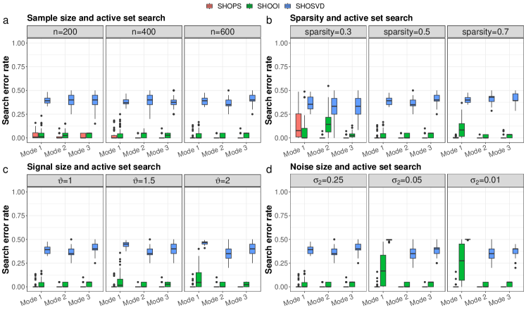
Figure 3: Active set search performances across different settings. a-d. Active set search error rates with varying sample size $n$, sparsity level, signal size $\vartheta$, and noise size $\sigma_{2}$. Each panel depicts a single set-up. The x-axis and y-axis represent tensor mode and search error rate, respectively. For each mode $M=1,2,3$, error rate is defined as $(FNR_{M}+FPR_{M})/2$, where $FNR_{M}=\frac{|\mathcal{A}_{M}^{*}\cap\hat{\mathcal{A}}_{M}^{C}|}{|\mathcal{A}_{M}^{*}|}$ and $FPR_{M}=\frac{|\mathcal{A}_{M}^{*C}\cap\hat{\mathcal{A}}_{M}|}{|\mathcal{A}_{M}^{*C}|}$. For SHOPS, $\nu$ is selected via cross-validation from $\nu\in\{0,0.1,\cdots,4\}$ and $K=2$, $R=2$. The results, where SHOPS uses GMM-based tuning for the thresholding parameter instead of CV are provided in Fig. LABEL:supp-fig:activeset_finding_gmm.

4.2 Estimation performances of SHOPS compared to alternative tensor Partial Least Squares models

Next, we compared SHOPS and a number of baseline PLS-based methods (summarized in Table LABEL:supp-tab:simul_methods) in terms of their estimation of the coefficient tensor and the mean response tensor as the sample size grows or as the sparsity level increases. We specifically considered two classes of tensor response regression models based on whether or not they imposed sparsity. For the first group of models, we considered the ordinary Higher Order Partial Least Squares (HOPLS) introduced in Section 2, and tensor response envelope model introduced in [17]. For the second group that incorporates sparsity, in addition to SHOPS, we devised two baseline alternatives by equipping Higher Order Partial Least Squares with two different active set finding algorithms: SHOSVD (SHOSVD-PLS) and SHOOI (SHOOI-PLS). Both SHOSVD-PLS and SHOOI-PLS directly extend the matrix SPLS [13] algorithm to the tensor response, and HOPLS is a modification of [14] with NIPALS PLS algorithm for theoretical guarantees under the non-sparse setting. Details of these baseline methods are presented in Algorithms LABEL:supp-alg:SHOSVD-PLS and LABEL:supp-alg:SHOOI-PLS, respectively.

[28] demonstrated that an envelope regression model coincides with finding an equivalent subspace of $\Sigma_{XX}$, where the envelope is the smallest reducing subspace of $\Sigma_{XX}$. While [16] introduced a tensor envelope partial least squares model for a tensor covariate $\mathcal{X}$ and vector response $Y$, this is not included in our benchmarking experiments because it does not accommodate tensor responses, which is our primary focus here. Instead, as a baseline method, we considered tensor response envelop model, even though it employs the smallest reducing subspace (envelope) of the covariance matrix of the vectorized error term $\mbox{vec}(\mathcal{E})$ and not of $\Sigma_{XX}$.

For these set of simulations, we considered sample sizes $n=100,200,\cdots,1000$, and $\mbox{sparsity}=0.1,0.2,\cdots,0.9$, and varied the sample size or the sparsity level while fixing the other parameters as in Section 4.1. For each specific setting, 40 simulation replicates were generated. We quantified the performances of the methods in two aspects with the following loss functions: $L_{1}=\frac{\left\lVert\hat{\mathcal{M}}-\mathcal{M}\right\rVert_{F}}{\left\lVert\mathcal{M}\right\rVert_{F}}$ and $L_{2}=\left\lVert\hat{\mathcal{B}}-\mathcal{B}\right\rVert_{F}$, where $\hat{\mathcal{B}}$ denotes the estimated coefficient tensor of $\mathcal{B}$, and $\hat{\mathcal{M}}=\hat{\mathcal{B}}\times_{1}X$ corresponds to the fitted values of the tensor regression for the true mean tensor $\mathcal{M}=\mathcal{B}\times_{1}X$. The first loss aims to quantify the estimation performance of $\mathcal{M}$, while the second quantifies the accuracy of the $\mathcal{B}$ estimation.

Fig. 4a,c display the performances of the methods across the simulation settings considered. These comparisons reveal that SHOPS is outperforming the alternatives in terms of the true mean estimation as SHOPS $L_{1}$ values are uniformly lower than the those of the other methods. In addition, the relative error decreases as the sparsity level increases for the methods that leverage sparsity (SHOPS, SHOOI-PLS, SHOSVD-PLS) with SHOPS exhibiting the smallest estimation error throughout the sparsity levels. In contrast, the non-sparse methods result in non-decreasing estimation errors with increasing sparsity levels. We note that SHOOI-PLS appears to have high $L_{1}$ value when the sparsity level is low, but converges to the level of SHOPS model as more than half of the coefficient tensor entries are zero (Fig. 4a). As the sample size increases, all the methods exhibit decreasing $L_{1}$ with SHOPS having the smallest error throughout the sample sizes (Fig. 4c). Envelope model results in large $L_{1}$ value when the sample size is low, but starts to perform as well as the sparse versions of the PLS models (SHOOI-PLS, SHOSVD-PLS) with increasing sample sizes, even though sparsity in not explicitly incorporated into its model.

When we compare the methods in terms of the estimation error $L_{2}=\left\lVert\hat{\mathcal{B}}-\mathcal{B}\right\rVert_{F}$ of the coefficient tensor, we observe that SHOPS results in the smallest error throughout the sparsity levels and sample sizes (Fig. 4b,d). As the sample size and the sparsity level increase, the SHOPS estimation error keeps decreasing, corroborating Theorem 3 for the consistency of the SHOPS estimator. Similar to the mean tensor estimation accuracy results, we observe that SHOOI-PLS tends to have high estimation error when the sparsity level is low, but converges to the error level of SHOPS model as the majority of the coefficient tensor entries become zero (Fig. 4b).

Overall, these simulation studies indicate that SHOPS correctly finds the active sets, and yields accurate estimation of the true mean tensor $\mathbb{E}[\mathcal{Y}]$ and the true coefficient $\mathcal{B}$. Furthermore, an extended version of the matrix SPLS algorithm [13], SHOOI-PLS, which we suggested here as a baseline without a theoretical guarantee, can also be employed along with SHOPS when we expect high levels of sparsity in the coefficient tensor.

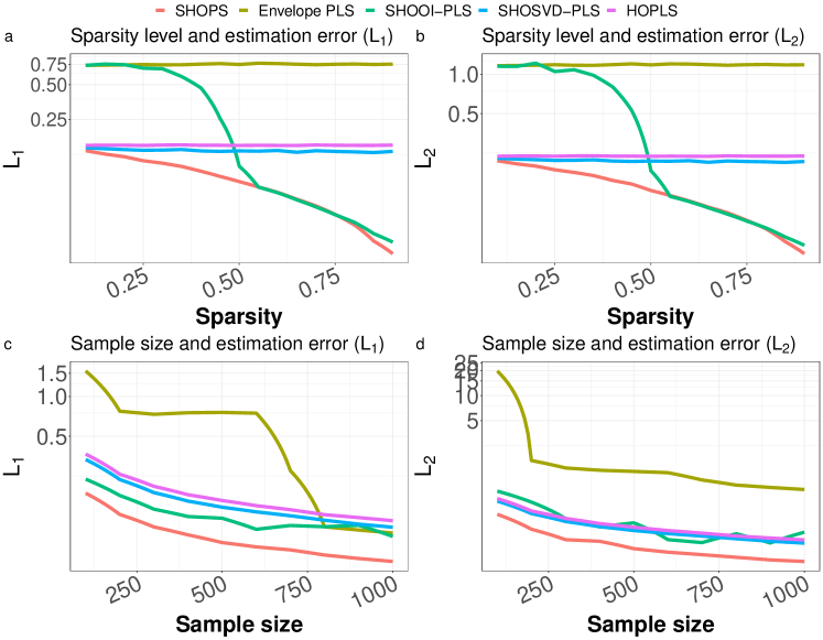
Figure 4: Estimation error performances for different settings. a,b. Estimation error $L_{1}=\frac{\left\lVert\hat{\mathcal{M}}-\mathcal{M}\right\rVert_{F}}{\left\lVert\mathcal{M}\right\rVert_{F}}$ and $L_{2}=\left\lVert\hat{\mathcal{B}}-\mathcal{B}\right\rVert_{F}$ for different PLS based methods under varying sparsity levels of the coefficient tensor. The x- and y-axis denote sparsity level and the loss value, respectively. c, d vary the sample size $n$. The results, where the SHOPS leverages GMM-based tuning instead of CV for the thresholding parameter is provided in Supplementary Materials Fig. LABEL:supp-fig:losses_gmm

5 Case studies

We next applied SHOPS to two different scientific problems. The first involves brain connectome mapping of the human cerebral cortex with magnetic resonance images [34] and the latter focuses on single cell-level chromatin conformation and DNA methylation levels of the genome as measured by the sn-m3C-seq assays [35]. Both of these settings harbor tensor responses and matrix covariates.

5.1 Application to brain connectome data

The Human Connectome Project (HCP) [34] generated brain network maps representing functional connectivity between brain regions of interest (i.e., brain nodes) with the broader goal of connecting brain’s structure to function and behavior. An HCP study by [36] generated data to probe relationships between brain connectivity and individual human characteristics (e.g., age, sex, cognitive and emotional traits). A subset of this dataset following the processing procedure of [37] is available through the R package tensorregress [38]. Specifically, the dataset contains symmetric adjacency matrices with a node size of 48 for 136 samples $(n=136)$. The entries of the adjacency matrix record functional connection between two brain nodes and give rise to a data structure with $d_{1}=136$, $d_{2}=d_{3}=48$. In addition, for each subject, Sex (Male or Female) and Age Group (Age 22-25, Age 26-30, Age 31+) are recorded. The key question of interest is to identify brain nodes that differ by Sex and/or Age Group. We used dummy variables to encode the female group, male group, Age 22-25, and Age 31+ without an intercept term ($p=4$). Hence, the baseline group for each sex group denotes the samples with Age 26-30. We labelled the group with Age 22-25 as ‘young’, and with Age 31+ as ‘old’ as a comparison to the baseline group.

We fit the SHOPS model by employing cross-validation for hyperparameter selection. Specifically, we used the screeplot of the eigenvalues of the sample covariance matrix of $X$ and selected the elbow point at $K_{max}=3$ as the maximum number of latent components $K$ for tuning with CV. We chose $R=3$ for the SHOPS active set finding algorithm, based on the minimum value of the elbow singular value points for all matricization of $S_{X\mathcal{Y}}$. Since the feature dimension $p$ is low, we did not impose sparsity on this mode. Hence, $T_{1r}=0$ for all $r\in[R]$. We let the rest of the modes of $\mathcal{B}$ be sparse by selecting the sparsity parameter $\nu$ from the set $\{0,0.2,0.4,\cdots,4\}$ with CV. The optimal values were set as $K=2$ and $\nu=2.6$ based on the 10-fold CV results.

Fig. 5 displays the estimated coefficient matrices on Desikan atlas brain template [37] from the SHOPS fit for the female group ($\hat{\mathcal{B}}_{[1,\,,\,]}-\hat{\mathcal{B}}_{[2,\,,\,]}$) and for the old group ($\hat{\mathcal{B}}_{[4,\,,\,]}$), i.e., edges with largest (top 3%) absolute effect sizes are displayed. We observe that the female group ($\hat{\mathcal{B}}_{[1,\,,\,]}-\hat{\mathcal{B}}_{[2,\,,\,]}$) has, on average, more connections between the two hemispheres of the brain than the male group (Fig. 5a). This finding is supported by the existing neuroscience literature. For example, [39] and [40] demonstrated that the brains of the females are more optimized for the inter-hemispheric connections and the related brain functions, while the male brains are more optimized for the intra-hemispheric connections.

Fig. 5b explores the aging effect on the brain connectome and reveals that nodes, specifically, Frontal-pole (Fploe), Cuneus, and Superior Temporal gyrus (SupT), Inferior Temporal gyrus (IT), in the old group are less connected than those of the younger groups. The largest effect of age is observed for the connection between the IT and SupT nodes. Inferior temporal gyrus is involved in memory and visual stimuli processing [41], and superior temporal gyrus plays a role in audio signal processing including languages [42]. These related traits are both known to be altered with aging.

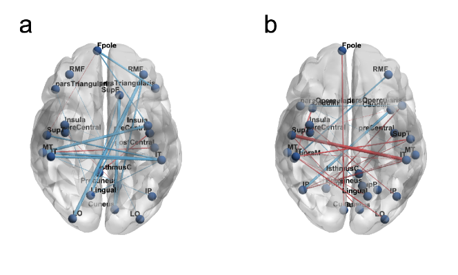
Figure 5: SHOPS estimated effects of sex and age on the brain connectome displayed on the Desikan atlas brain template. a. Visual representation of the differences of the estimated sex effects (Fig. LABEL:supp-fig:brain_adjc) on the brain connectome ($\hat{\mathcal{B}}_{[1,\,,\,]}-\hat{\mathcal{B}}_{[2,\,,\,]}$). b Visual representation of the estimated age effect (Fig. LABEL:supp-fig:brain_adjd) on the brain connectome. Displayed is $\hat{\mathcal{B}}_{[4,\,,\,]}$ which denotes the difference between old group (31+) and the reference group (22-25). For both of the panels, the width of each line connecting two nodes correspond to the absolute effect size, while the color of the lines denotes the sign of the effect (red: negative, blue: positive).

5.2 Application to sn-m3C-seq data of adult mouse hippocampus

sn-m3C-seq assay is a multi-omics assay that simultaneously profiles long-range chromatin contacts (i.e., Hi-C for high throughput chromosome conformation capture) and DNA methylation (epigenomics) at the single cell level [43, 35]. Both long-range contacts of the genome and DNA methylation are key components of regulation of gene expression. We showcase application of SHOPS to investigate how long-range chromatin contacts relate to methylation across genomic loci with sn-m3C-seq data from adult mouse hippocampus [35]. We refer to the long-range chromatin contact portion of the data as scHi-C (single cell Hi-C) for short.

Following the third order tensor viewpoint of [25] on scHi-C data, for a single cell $i\in[n]$, we have 20 chromosomes (for mouse genome) and a Hi-C contact matrix of size $d_{2,chr}\times d_{3,chr}$ for each $chr\in[20]$. Each $(j,k)$-th entry of a contact matrix denotes the contact counts that quantify the level of physical contact between genomic loci $j\in[d_{2,chr}]$ and $k\in[d_{3,chr}]$. When the contact matrices are stacked along cells $(n=711)$, the scHi-C data can be viewed as a third order tensor $\mathcal{Y}_{chr}\in\mathbb{R}^{n\times d_{2,chr}\times d_{3,chr}}$ for each chromosome $chr\in[20]$. While the contact matrices traditionally have "bins" (intervals of size 1Kb-1Mb tiling the genome) as rows and columns, we subset these to include genes and enhancers in order to constrain the second and third modes of the tensor to known functional units of the genome. Specifically, the second mode of a chromosome-specific tensor is defined as the genes residing on the chromosome and the third mode is defined as the enhancers, which are typically noncoding regions within $\pm$ 1Mb of the genes and play essential roles in regulating the genes. Hence, $d_{2,chr}$ denotes the number of genes and $d_{3,chr}$ denotes the number of enhancers. In addition, for a chromosome $chr\in[20]$ within each cell $i\in[n]$, we have DNA methylation level profiled throughout $p_{chr}$ genomic loci, i.e., methylation covariate matrix $X_{chr}\in\mathbb{R}^{n\times p_{chr}}$.

The original publication of [35] provided cell type labels of the cells profiled. Using this labelling information, we created a response tensor $\mathcal{Y}_{chr}$ using genes with differential contact levels throughout four cell types of interest: CA3, MGC, OPC, and VLMC. While our initial set of enhancers harbored the enhancers existing in gene-cCRE (cis-regulatory elements) correlation lists summarized by [44], we further subsetted these enhancers and kept the ones with differential methylation levels throughout the four cell types. The methylation covariate matrix $X_{chr}$ was also subsetted to include the same set of enhancers. Further details about data processing, including data normalization and differential analysis are provided in Supplementary Materials Section LABEL:supp-preprocess.

SHOPS analysis identifies gene-enhancer regulatory relations. To elucidate how the DNA methylation level at enhancers affects the physical contact between genes and enhancers, we fitted the SHOPS model $\mathcal{Y}_{chr}=\mathcal{B}_{chr}\times_{1}X_{chr}+\mathcal{E}_{chr}$ for each chromosome $chr$ separately. To the best of our knowledge, this work is the first to investigate the impact of methylation on long-range contacts with a tensor regression approach. Therefore, we will further elaborate on what the model aims to capture.

Firstly, we note that for $\mathcal{B}_{chr}\in\mathbb{R}^{p_{chr}\times d_{2,chr}\times d_{3,chr}}$, a tensor fiber $\mathcal{B}_{chr[i,\,,i]}\in\mathbb{R}^{d_{2,chr}}$ represents the effect of DNA methylation at enhancer $i$ on the contact between that enhancer (enhancer $i$) and genes. If gene $g$ has a large coefficient value $\mathcal{B}_{chr[i,g,i]}$, this implies that the methylation of enhancer $i$ affects its physical contact with gene $g$, and that enhancer $i$ is a potential regulator of the gene $g$ (Fig. 6). Fig. 7a visualizes the tensor fiber $\hat{\mathcal{B}}_{chr[i,\,,i]}$ for $i$-th enhancer located at chr2:157,463,107-157,463,914, and reveals that methylation at this enhancer affects the physical contact of the enhancer with gene Src the most, compared to other genes. This suggests that the enhancer is a potential regulator of the gene Src, which is proximal to the enhancer in genomic location. SHOPS model facilitates such gene selection by imposing sparsity along the gene mode. Fig. 7b reveals that SHOPS thresholded out other genes that are farther away from the enhancer in genomic location even though they exhibited non-zero covariance in the corresponding fiber of the covariance tensor $S_{X\mathcal{Y}}$.

In order to validate that non-zero entries of the estimated $\mathcal{B}_{chr[i,\,,i]}$ fiber, $i=1\cdots,J_{chr}$, suggest gene regulation by enhancer $i$, we compared these non-zero entry sets against the external gene-enhancer co-accessibility matrix provided by [44]. Gene-enhancer co-accessibility is inferred from another type of single cell profiling assay named sn-ATAC-seq and is a proxy that is commonly used to link enhancers to genes [45]. It operates on the assumption that if an enhancer is a regulator of a gene, the enhancer and the promoter region of the gene would exhibit co-accessibility across the cells. However, the reverse is not necessarily true. We considered 41,304 g-e (gene-enhancer) pairs across all chromosomes that were both part of our analysis and in the co-accessibility matrix. Next, we identified the g-e pairs with significant co-accessibility at false discovery rate (FDR) of 0.05 using the statistical analysis results that were reported by the co-accessibility analysis of [44]. We further defined $A_{1}=\{\mbox{g-e pairs with significant co-accessibility at FDR 0.05}\}$, and $A_{2}=\{\mbox{g-e pairs with non zero }\hat{\mathcal{B}}_{chr[i,\,,i]}\}$.

Fig. 7c displays the overlap between these two sets across all chromosomes and highlights that majority of the g-e links identified by SHOPS $(A_{2})$ have significant g-e co-accessibility at FDR of 0.05, i.e., about 65% of the $A_{2}$ set g-e pairs are among the $A_{1}$ set. In contrast, the reverse does not hold, i.e., only a small proportion of $A_{1}$ set g-e pairs are among the $A_{2}$ set. This aligns with the intuition that g-e co-accessibility does not necessarily imply long-range contacts. Such correlations in co-accessibility could arise due to co-expressed genes (i.e., when two genes are co-expressed, accessibility of their enhancers could correlate with each other’s promoter accessibility).

Next, to further validate that the g-e pairs within $A_{2}$ are better supported compared to those within $A_{1}$, we compared their scHi-C contact counts. Overall, we would expect that the contact level between a gene and its regulator is higher than the contacts between the gene and a non-regulating enhancer [46, 47], hence leading to higher contact counts. First, Fig. 7d yields that the contact counts of g-e pairs in the intersection, g-e $\in A_{1}\cap A_{2}$, is significantly higher than those pairs specific to $A_{1}$, g-e $\in A_{1}-A_{2}$ ($\mbox{p-value}<2.9e-06$). Furthermore, we also observe that contact counts for g-e pairs that are specific to $A_{2}$ (g-e $\in A2-A1$) are also higher than those pairs specific to $A_{1}$, further consolidating the results of the co-accessibility analysis.

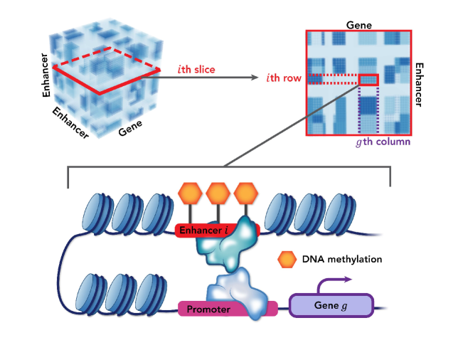
Figure 6: Interpretation of super-diagonal entries of the coefficient tensor $\mathcal{B}_{chr}$ for SHOPS application to sn-m3C-seq data of [35]. The coefficient tensor $\mathcal{B}_{chr}$ depicted in the top left panel denotes an enhancer ($p_{chr}$)$\times$gene ($d_{2chr}$)$\times$enhancer ($d_{3chr}$) tensor. The $i$th slice of the first mode of the coefficient tensor $\mathcal{B}_{chr}$ summarizes the effect of DNA methylation at enhancer $i$ on the contact level between the enhancers and the genes on the chromosome $chr$ (top right panel). On the $i$th slice of the coefficient tensor, each entry in the $i$th row depicts the effect of DNA methylation at enhancer $i$ on the contact between the enhancer $i$ and a gene. Specifically, as the bottom panel depicts, DNA methylation (orange hexagons) at enhancer $i$ (red box) influences the contact between the target gene $g$ (purple box) and enhancer $i$. The square box entry of the top right panel shows the effect size.

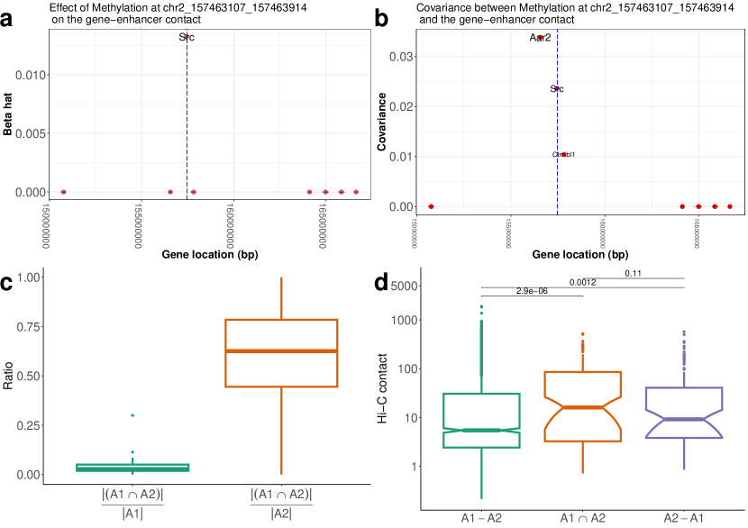
Figure 7: Gene regulatory elements and SHOPS estimator. a,b. Dot plot of $\hat{\mathcal{B}}_{2[i,\,,i]}$ ($S_{X\mathcal{Y}2[i,\,,i]}$) fiber. x-axis denotes the genomic location of genes (10 Mega base pair (Mbp) around the gene), and the y-axis denotes the coefficient (covariance) value on the fiber, which summarizes the association level between the DNA methylation level at the $i$th enhancer (blue vertical line) and the physical contact of a gene (red dot) and the enhancer $i$. c. Boxplots depicting the overlap rates $|A_{1}\cap A_{2}|/|A_{1}|$ and $|A_{1}\cap A_{2}|/|A_{2}|$. d. Boxplots depicting the scHi-C contact levels for the g-e pairs in each of $A_{1}-A_{2},A_{1}\cap A_{2},A_{2}-A_{1}$. For c,d g-e pairs in all the chromosomes are considered, and for d, the contact levels are normalized so that the contact level is not biased by gene or enhancer length.

SHOPS analysis identifies multi-way regulatory relations. Thus far, we evaluated the SHOPS results in terms of the impact of methylation of an enhancer to that enhancer’s contacts with the genes. However, SHOPS analysis also generates candidates of multi-way contacts (i.e., also known as many-body interactions [48, 49]) in the genome. Such multi-way contacts arise when a gene is regulated by multiple interacting enhancers. The SHOPS coefficient entry $\mathcal{B}_{chr[i,g,j]}$ can be interpreted as the effect of methylation at $i$th enhancer on the contact count between gene $g$ and enhancer $j$ (Fig. 8). For example, Fig. 9a,b display an estimated tensor slice $\hat{\mathcal{B}}_{chr[i,\,,\,]}$ for two enhancers (a for enhancer located at chr2:130,382,900-130,384,345, b for enhancer located at chr2:130,513,148-130,513,733). Fig. 9a yields that the methylation at enhancer located at chr2:130,382,900-130,384,345 (marked with a green vertical line) affects the contact between gene Ptpra and the enhancer chr2:130,429,699-130,430,418 (red rectangular box intersecting with red vertical line). While these two enhancers marked in Fig. 9a are close to each in their genomic coordinates, this type of three-way contact could also occur among enhancer elements that are distal to each other (Fig. 9b).

As we demonstrated previously, the g-e pairs with non-zero estimated coefficients in the $\hat{\mathcal{B}}_{chr[i,\,,i]}$ fiber have significantly higher contact counts compared to the others (boxplot for Intra group in Fig. 9b). To further validate enhancer-enhancer contacts in the inferred g-e-e triplet (gene $g$, enhancer $i$, enhancer $j$), we quantified the contact counts between the two enhancers ($i$ and $j$) (boxplot across chromosomes for Inter group in Fig. 9b) and observed that these enhancers harbor significantly more contact counts than enhancers that are not inferred to interact by SHOPS (Wilcoxon ranksum test p-value of $0.035$ with Benjamini-Hochberg [50] correction). Moreover, there are about $50\%$ more zero scHi-C contact counts in the random enhancers (Other group) than the multi-way interacting enhancers (Inter group).

In summary, SHOPS model applied to sn-m3C-seq data has the potential to reveal both enhancers of genes and multi-way contacts involving multiple enhancers.

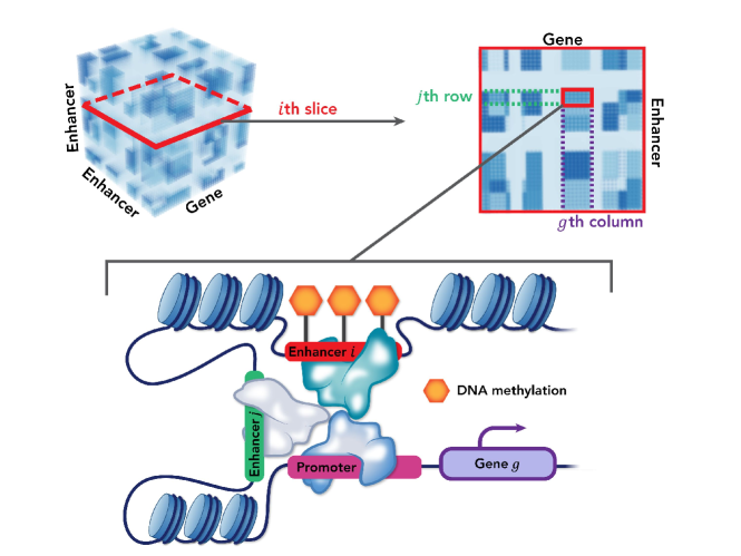
Figure 8: Interpretation of off-diagonal entries of the coefficient tensor $\mathcal{B}_{chr}$ and multi-way contacts. The top two panels are equivalent to those of Fig. 6. On the $i$th slice of the coefficient tensor, each entry in the $j$th row depicts the effect of DNA methylation at enhancer $i$ on the contact count between the $j$th enhancer and a gene. Specifically, as the bottom panel shows, DNA methylation (orange hexagons) at an enhancer $i$ (red box) influences the contact between another enhancer $j$ (yellow box) and the target gene $g$ (purple box), which indicates a multi-way contact in the chromatin. The square box entry of the top right panel depicts the effect size.

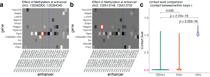
Figure 9: a.b, SHOPS estimates for the coefficient slice matrix $\mathcal{B}_{2[i,\,,\,]}$. x-axis denotes the enhancers within 2Mbp region around the $i$th enhancer (a. chr2:130,382,900-130,384,345, b. chr2:130,513,148-130,513,733) and y-axis lists the nearby genes. Each entry of the matrix denotes the estimated coefficient value (darker values correspond to larger values). Green vertical line denotes the location of the enhancer $i$, blue (red) vertical line denotes the location of enhancer with the maximum (minimum) estimated coefficient in the matrix. c. scHi-C contact levels (normalized as in Fig. 7) of the three groups of genomic regions Intra: gene-enhancer pairs with non-zero estimated $\mathcal{B}_{chr[i,\,,i]}$ values for all $i$, $chr$. Inter: enhancer_i-enhancer_j pairs, where enhancer_j has the maximum effect size in absolute value in the estimated $\mathcal{B}_{chr[i,\,,\,]}$ matrix for each $i$, $chr$. Others: enhancer-enhancer pairs excluding Inter group pairs. Since the Intra group has disproportionately large contact levels, all the contact levels are transformed with $x^{1/25}$ to visualize the three groups in one plot. Each pairs of groups is compared with the Wilcoxon rank sum test.

6 Discussion

In this paper, we presented SHOPS model for simultaneous dimension reduction of the high-dimensional predictor variables, selection of important variables, and tensor response denoising. Theoretical investigations of the SHOPS model and the simulation studies illustrated that SHOPS yields $\sqrt{n}-$consistent estimator $\hat{\mathcal{B}}_{SHOPS}$ even under the high-dimensional regime, where $n\ll pd_{2}d_{3}$. It is worthwhile to note that Algorithm 3 that identifies correct active sets with high probability plays a crucial role in establishing such a consistency result for SHOPS. Application of SHOPS to real datasets highlighted the utility of SHOPS for modern high-dimensional tensor response regression problems. Specifically, the HCP [34] application revealed the sex and age specific brain connectivity patterns that aligned well with the current neuroscience literature. Application to sn-m3C-seq [43] (scHi-C + scMethyl) data revealed SHOPS as identifying regulatory elements of genes and multi-way interactions among genes and two different enhancers. The latter is a relatively less explored area of single cell genomics.

This work establishes sparse tensor response partial least squares method as a modeling approach in the high-dimensional tensor response and matrix covariate settings. Moreover, it also addresses the consistency rates of the tensor (multivariate) response (both sparse or non-sparse) partial least squares regression when both the dimensions on response tensor and the numbers of predictors increase. While [13] and [29] provide consistency result of the multivariate response partial least squares, they rely on the assumption that the dimensionality of the response matrix is fixed, which is a restrictive assumption in modern applications arising from HCP and single cell genomics. In addition to the SHOPS algorithm with theoretical guarantee, we also devised two baseline algorithms: SHOSVD-PLS (Algorithm LABEL:supp-alg:SHOSVD-PLS) and SHOOI-PLS (Algorithm LABEL:supp-alg:SHOOI-PLS). These algorithms are direct tensor extensions of the SPLS algorithm of [13]. Interestingly, SHOOI-PLS empirically achieves comparable performance to SHOPS, even though it lacks theoretical justification.

While this paper provides theoretical guarantees related to active set recovery and consistency of the sparse higher order partial least squares model, existing proposition about the equivalence between PLS and envelope regression by [28] implies that an envelope extension of the SHOPS model could potentially achieve asymptotic normality of the estimator $\hat{\mathcal{B}}$, which would enable statistical inferences including testing and confidence intervals. In addition, we employed Gaussian noise model on the response $\mathcal{Y}$, but a natural extension to the sub-Gaussian GLM model can be made similar to the extension obtained by [51, 29]. In addition to the sub-Gaussian extension of SHOPS, inference on other parameters of the response tensor could also be obtained. For example, we expect that the PLS or envelope framework on the quantile regression [52, 53] and tensor regression viewpoint on the quantile regresion [54] joined together could make SHOPS applicable for quantile estimation of the high-dimensional response variables.

7 Competing interests

No competing interest is declared.

8 Author contributions statement

K.P. and S.K. conceived the project. K.P. developed the methodology and theory, and conducted the computational experiments under supervision from S.K. K.P. and S.K. wrote the manuscript.

9 Acknowledgments

This work is supported in part by funds from the National Institutes of Health (NIH: R01HG003747, R21HG012881) and Chan Zuckerberg Initiative Data Insights Ward.

References

- [1] Tibshirani, R.: Regression shrinkage and selection via the lasso. Journal of the Royal Statistical Society: Series B (Methodological) 58(1), 267–288 (1996)
- [2] Fan, J., Li, R.: Variable selection via nonconcave penalized likelihood and its oracle properties. Journal of the American statistical Association 96(456), 1348–1360 (2001)
- [3] Efron, B., Hastie, T., Johnstone, I., Tibshirani, R.: Least angle regression (2004)
- [4] Zou, H., Hastie, T.: Regression shrinkage and selection via the elastic net, with applications to microarrays. JR Stat Soc Ser B 67, 301–20 (2003)
- [5] Tibshirani, R., Saunders, M., Rosset, S., Zhu, J., Knight, K.: Sparsity and smoothness via the fused lasso. Journal of the Royal Statistical Society Series B: Statistical Methodology 67(1), 91–108 (2005)
- [6] Yuan, M., Lin, Y.: Model selection and estimation in regression with grouped variables. Journal of the Royal Statistical Society: Series B (Statistical Methodology) 68(1), 49–67 (2006)
- [7] Raskutti, G., Wainwright, M.J., Yu, B.: Minimax rates of estimation for high-dimensional linear regression over -balls. IEEE transactions on information theory 57(10), 6976–6994 (2011)
- [8] Hastie, T., Tibshirani, R., Wainwright, M.: Statistical learning with sparsity: the lasso and generalizations. CRC press (2015)
- [9] Li, J., Cheng, K., Wang, S., Morstatter, F., Trevino, R.P., Tang, J., Liu, H.: Feature selection: A data perspective. ACM computing surveys (CSUR) 50(6), 1–45 (2017)
- [10] Wold, H.: Estimation of principal components and related models by iterative least squares. Multivariate analysis pp. 391–420 (1966)
- [11] De Jong, S.: Simpls: an alternative approach to partial least squares regression. Chemometrics and intelligent laboratory systems 18(3), 251–263 (1993)
- [12] Helland, I.S., Almøy, T.: Comparison of prediction methods when only a few components are relevant. Journal of the American Statistical Association 89(426), 583–591 (1994)
- [13] Chun, H., Keleş, S.: Sparse partial least squares regression for simultaneous dimension reduction and variable selection. Journal of the Royal Statistical Society: Series B (Statistical Methodology) 72(1), 3–25 (2010)
- [14] Zhao, Q., Caiafa, C.F., Mandic, D.P., Chao, Z.C., Nagasaka, Y., Fujii, N., Zhang, L., Cichocki, A.: Higher order partial least squares (hopls): A generalized multilinear regression method. IEEE transactions on pattern analysis and machine intelligence 35(7), 1660–1673 (2012)
- [15] Rabusseau, G., Kadri, H.: Low-rank regression with tensor responses. Advances in Neural Information Processing Systems 29 (2016)
- [16] Zhang, X., Li, L.: Tensor envelope partial least-squares regression. Technometrics 59(4), 426–436 (2017)
- [17] Li, L., Zhang, X.: Parsimonious tensor response regression. Journal of the American Statistical Association 112(519), 1131–1146 (2017)
- [18] Sun, W.W., Li, L.: Store: sparse tensor response regression and neuroimaging analysis. The Journal of Machine Learning Research 18(1), 4908–4944 (2017)
- [19] Lock, E.F., Li, G.: Supervised multiway factorization. Electronic journal of statistics 12(1), 1150 (2018)
- [20] Raskutti, G., Yuan, M., Chen, H.: Convex regularization for high-dimensional multiresponse tensor regression (2019)
- [21] Kolda, T.G., Bader, B.W.: Tensor decompositions and applications. SIAM review 51(3), 455–500 (2009)
- [22] De Lathauwer, L., De Moor, B., Vandewalle, J.: On the best rank-1 and rank-(r 1, r 2,…, rn) approximation of higher-order tensors. SIAM journal on Matrix Analysis and Applications 21(4), 1324–1342 (2000)
- [23] Johnstone, I.M., Lu, A.Y.: On consistency and sparsity for principal components analysis in high dimensions. Journal of the American Statistical Association 104(486), 682–693 (2009)
- [24] Naik, P., Tsai, C.L.: Partial least squares estimator for single-index models. Journal of the Royal Statistical Society: Series B (Statistical Methodology) 62(4), 763–771 (2000)
- [25] Park, K., Keles, S.: Joint tensor modeling of single cell 3D genome and epigenetic data with Muscle. bioRxiv pp. 2023–01 (2023)
- [26] Deshpande, Y., Montanari, A.: Sparse pca via covariance thresholding. Advances in Neural Information Processing Systems 27 (2014)
- [27] Cai, T., Ma, Z., Wu, Y.: Sparse PCA: Optimal Rates and Adaptive Estimation. The Annals of Statistics 41 (Nov 2012)
- [28] Cook, R.D., Helland, I., Su, Z.: Envelopes and partial least squares regression. Journal of the Royal Statistical Society: SERIES B: Statistical Methodology pp. 851–877 (2013)
- [29] Zhu, G., Su, Z.: Envelope-based sparse partial least squares (2020)
- [30] Wang, Z., Gu, Q., Ning, Y., Liu, H.: High dimensional em algorithm: Statistical optimization and asymptotic normality. In: Cortes, C., Lawrence, N., Lee, D., Sugiyama, M., Garnett, R. (eds.) Advances in Neural Information Processing Systems. vol. 28. Curran Associates, Inc. (2015), https://proceedings.neurips.cc/paper_files/paper/2015/file/1415db70fe9ddb119e23e9b2808cde38-Paper.pdf
- [31] De Lathauwer, L., De Moor, B., Vandewalle, J.: A multilinear singular value decomposition. SIAM journal on Matrix Analysis and Applications 21(4), 1253–1278 (2000)
- [32] Yang, D., Ma, Z., Buja, A.: A sparse singular value decomposition method for high-dimensional data. Journal of Computational and Graphical Statistics 23(4), 923–942 (2014)
- [33] Zhang, A., Han, R.: Optimal sparse singular value decomposition for high-dimensional high-order data. Journal of the American Statistical Association 114(528), 1708–1725 (2019)
- [34] Van Essen, D.C., Smith, S.M., Barch, D.M., Behrens, T.E., Yacoub, E., Ugurbil, K., Consortium, W.M.H., et al.: The wu-minn human connectome project: an overview. Neuroimage 80, 62–79 (2013)
- [35] Liu, H., Zhou, J., Tian, W., Luo, C., Bartlett, A., Aldridge, A., Lucero, J., Osteen, J.K., Nery, J.R., Chen, H., et al.: Dna methylation atlas of the mouse brain at single-cell resolution. Nature 598(7879), 120–128 (2021)
- [36] Barch, D.M., Burgess, G.C., Harms, M.P., Petersen, S.E., Schlaggar, B.L., Corbetta, M., Glasser, M.F., Curtiss, S., Dixit, S., Feldt, C., et al.: Function in the human connectome: task-fmri and individual differences in behavior. Neuroimage 80, 169–189 (2013)
- [37] Desikan, R.S., Ségonne, F., Fischl, B., Quinn, B.T., Dickerson, B.C., Blacker, D., Buckner, R.L., Dale, A.M., Maguire, R.P., Hyman, B.T., et al.: An automated labeling system for subdividing the human cerebral cortex on mri scans into gyral based regions of interest. Neuroimage 31(3), 968–980 (2006)
- [38] Hu, J., Lee, C., Wang, M.: Generalized tensor decomposition with features on multiple modes. Journal of Computational and Graphical Statistics 31(1), 204–218 (2022)
- [39] Ingalhalikar, M., Smith, A., Parker, D., Satterthwaite, T.D., Elliott, M.A., Ruparel, K., Hakonarson, H., Gur, R.E., Gur, R.C., Verma, R.: Sex differences in the structural connectome of the human brain. Proceedings of the National Academy of Sciences 111(2), 823–828 (2014)
- [40] Tunç, B., Solmaz, B., Parker, D., Satterthwaite, T.D., Elliott, M.A., Calkins, M.E., Ruparel, K., Gur, R.E., Gur, R.C., Verma, R.: Establishing a link between sex-related differences in the structural connectome and behaviour. Philosophical Transactions of the Royal Society B: Biological Sciences 371(1688), 20150111 (2016)
- [41] Kolb, B., Whishaw, I.Q., Teskey, G.C., Whishaw, I.Q., Teskey, G.C.: An introduction to brain and behavior. Worth New York (2001)
- [42] Bigler, E.D., Mortensen, S., Neeley, E.S., Ozonoff, S., Krasny, L., Johnson, M., Lu, J., Provencal, S.L., McMahon, W., Lainhart, J.E.: Superior temporal gyrus, language function, and autism. Developmental neuropsychology 31(2), 217–238 (2007)
- [43] Lee, D.S., Luo, C., Zhou, J., Chandran, S., Rivkin, A., Bartlett, A., Nery, J.R., Fitzpatrick, C., O’Connor, C., Dixon, J.R., et al.: Simultaneous profiling of 3d genome structure and dna methylation in single human cells. Nature methods 16(10), 999–1006 (2019)
- [44] Li, Y.E., Preissl, S., Hou, X., Zhang, Z., Zhang, K., Qiu, Y., Poirion, O.B., Li, B., Chiou, J., Liu, H., et al.: An atlas of gene regulatory elements in adult mouse cerebrum. Nature 598(7879), 129–136 (2021)
- [45] Pliner, H.A., Packer, J.S., McFaline-Figueroa, J.L., Cusanovich, D.A., Daza, R.M., Aghamirzaie, D., Srivatsan, S., Qiu, X., Jackson, D., Minkina, A., et al.: Cicero predicts cis-regulatory dna interactions from single-cell chromatin accessibility data. Molecular cell 71(5), 858–871 (2018)
- [46] Miele, A., Dekker, J.: Long-range chromosomal interactions and gene regulation. Molecular biosystems 4(11), 1046–1057 (2008)
- [47] Schoenfelder, S., Fraser, P.: Long-range enhancer–promoter contacts in gene expression control. Nature Reviews Genetics 20(8), 437–455 (2019)
- [48] Perez-Rathke, A., Sun, Q., Wang, B., Boeva, V., Shao, Z., Liang, J.: Chromatix: computing the functional landscape of many-body chromatin interactions in transcriptionally active loci from deconvolved single cells. Genome biology 21(1), 1–17 (2020)
- [49] Liu, L., Zhang, B., Hyeon, C.: Extracting multi-way chromatin contacts from hi-c data. PLoS Computational Biology 17(12), e1009669 (2021)
- [50] Benjamini, Y., Hochberg, Y.: Controlling the false discovery rate: a practical and powerful approach to multiple testing. Journal of the Royal statistical society: series B (Methodological) 57(1), 289–300 (1995)
- [51] Chung, D., Keles, S.: Sparse partial least squares classification for high dimensional data. Statistical applications in genetics and molecular biology 9(1) (2010)
- [52] Dodge, Y., Whittaker, J.: Partial quantile regression. Metrika 70, 35–57 (2009)
- [53] Ding, S., Su, Z., Zhu, G., Wang, L.: Envelope quantile regression. Statistica Sinica 31(1), 79–105 (2021)
- [54] Li, C., Zhang, H.: Tensor quantile regression with application to association between neuroimages and human intelligence. The Annals of Applied Statistics 15(3), 1455–1477 (2021)