Unveiling UV/IR Mixing via Symmetry Defects:
A View from Topological Entanglement Entropy

Abstract

Some topological lattice models in two spatial dimensions have been found to exhibit intricate system size dependence in their ground state degeneracy (GSD), often known as UV/IR mixing. We distinguish between two explanations for this phenomenon by explicitly calculating the topological entanglement entropy (TEE) of a model system, the rank-2 toric code, for a bi-partition of the torus into two cylinders. Focusing on the fact that the rank-2 toric code is a translation symmetry-enriched topological phase, we show that viewing distinct system sizes as different translation symmetry defects can explain both our TEE results and the GSD of the rank-2 toric code. Our work establishes the symmetry defect framework as the most complete description of this system size dependence.

In the realm of topological order in two dimensions, one may observe the emergence of anyonic excitations characterized by their anyonic braiding statistics and the topology-dependent ground state degeneracy (GSD) Wen (2007); Kitaev (2003). In the presence of symmetry, the structure of topological order becomes even richer as there can be multiple distinct “symmetry-enriched topological phases” (SETs) with the same anyons and statistics Wen (2002); Kou and Wen (2009); Essin and Hermele (2013); Mesaros and Ran (2013); Stephen et al. (2020); Lu and Vishwanath (2016). SETs exhibit symmetry fractionalization Wen (2002); Chen (2017), wherein the emergent quasiparticles transform projectively under the symmetry operations. Furthermore, the symmetry may non-trivially permute the topological superselection sectors, which is denoted as anyonic symmetry Lu and Vishwanath (2016); Barkeshli et al. (2019); Tarantino et al. (2016).

Normally, the GSD of a topologically ordered system on a torus depends only on the number of distinct anyon types, which is independent of the system size. However, several models in which the GSD depends sensitively on the size of the torus have been discussed recently Wen (2003); You and Wen (2012); Gorantla et al. (2021, 2022, 2023); Oh et al. (2022a, b, 2023); Pace and Wen (2022); Delfino et al. (2023a, b); Ebisu (2023a, b); Watanabe et al. (2023). For example, the $\mathbb{Z}_{N}$ plaquette model Wen (2003); You and Wen (2012) has a GSD which depends on whether the linear dimension is even or odd, while other $\mathbb{Z}_{N}$ models have GSDs that depend on the linear dimension modulo $N$. This system size dependence has sometimes been viewed as a signature of so-called UV/IR mixing, in the sense that microscopic information (namely the lattice constant) affects the low-energy properties of the model.

There have been two primary explanations for the mechanism by which the system size affects the low-energy properties of topologically ordered systems. One Pace and Wen (2022); Gorantla et al. (2022) is to view certain locally inequivalent configurations of excitations as globally equivalent thanks to processes that take place over the entire linear size of the system. Another Watanabe et al. (2023) emphasizes the fact that these systems are translation SETs and views the system size dependence as arising from translation symmetry defects threaded through non-contractible spatial cycles. Both of these explanations have been used to quantitatively explain the topological GSD of lattice anyon models.

In this work, we show that for one such model, the symmetry defect approach can explain not only the GSD but also the topological entanglement entropy (TEE) for the bi-partition of the torus into two cylinders Levin and Wen (2006); Kitaev and Preskill (2006); Zhang et al. (2012); Teo et al. (2015). This is strong evidence for the usefulness of the defect approach because if the entanglement cut has non-contractible loops, then the TEE allows us to directly extract the quantum dimension of symmetry defects. In contrast, because this TEE explicitly incorporates one periodic boundary condition but not the other, it is much less natural to justify the torus TEE via some global relation between superselection sectors. The model we choose is the $\mathbb{Z}_{N}$ rank-2 toric code (R2TC) Bulmash and Barkeshli (2018); Oh et al. (2022a); Pace and Wen (2022); Oh et al. (2022b, 2023). We match our explicit calculation of the TEE and known results about the GSD to quantitative predictions from the theory of symmetry defects in SETs Barkeshli et al. (2019); Tarantino et al. (2016); Turaev (2000); Etingof et al. (2010). From this perspective, different linear system sizes modulo $N$ are viewed as having different symmetry defects threaded through a handle of the torus.

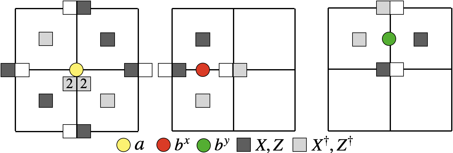
Figure 1: Three stabilizers $a_{i}$, $b_{i}^{x}$, and $b_{i}^{y}$ of R2TC are depicted as yellow, red, and green symbols, respectively. The $a_{i}$ stabilizer is a product of $\mathbb{Z}_{N}$ Pauli-$Z$ operators, while $b_{i}^{x}$ and $b_{i}^{y}$ consist of $\mathbb{Z}_{N}$ Pauli-$X$ operators. There are two $\mathbb{Z}_{N}$ spins defined at the vertices (represented by two adjacent squares) and one $\mathbb{Z}_{N}$ spin (represented by a single square) at the plaquette centers of the square lattice. The ‘2’ inside the squares on the far left figure implies the action by $(Z^{\dagger})^{2}$ for both spins. The empty square means there is no action by Pauli operators on that spin.

The R2TC is a generalization of the Kitaev toric code consisting of three types of stabilizers called $a_{i}$, $b^{x}_{i}$, and $b^{y}_{i}$, defined respectively around the site $i$ and the two links $(i,i+\hat{x})$, and $(i,i+\hat{y})$ on a square lattice as shown in Fig. 1. At each site we have two $\mathbb{Z}_{N}$ degrees of freedom, denoted by subscripts $1$ and $2$, with an additional $\mathbb{Z}_{N}$ degree of freedom at the center of each plaquette denoted by the subscript $0$. Using these $\mathbb{Z}_{N}$ spins we can construct the three stabilizers as depicted in Fig. 1. The stabilizer $a_{i}$ is a product of $\mathbb{Z}_{N}$ Pauli-$Z$ operators, while $b_{i}^{x}$ and $b_{i}^{y}$ are products of $\mathbb{Z}_{N}$ Pauli-$X$ operators, which form the algebra $Z_{i,a}X_{j,b}=\omega\delta_{ij}\delta_{ab}X_{j,b}Z_{i,a}$, where $a,b=0,1,2$ and $\omega=e^{2\pi i/N}$. The ground state(s) is an eigenstate of all the stabilizers with the eigenvalue +1. Excitations of this model are anyons carrying position-dependent labels; following Pace and Wen (2022), one can label the distinct anyon types at the site $(i_{x},i_{y})$ using the formula

$$l_{i_{x},i_{y}} =l_{1}\mathtt{e}+(l_{1}i_{x}+l_{2}~{}{\rm mod}~{}N)\mathtt{p}^{x}$$

$$+(l_{1}i_{y}+l_{3}~{}{\rm mod}~{}N)\mathtt{p}^{y}$$

$$+l_{4}\mathtt{m}^{x}+l_{5}\mathtt{m}^{y}+(l_{4}i_{y}+l_{5}i_{x}+l_{6}~{}{\rm mod}~{}N)\mathtt{g}.$$ (1)

Here $(\mathtt{e},\mathtt{p}^{x},\mathtt{p}^{y},\mathtt{m}^{x},\mathtt{m}^{y},\mathtt{g})$ are six distinct Abelian anyon types which generate all of the anyons in the model. An excited $a$ stabilizer on lattice sites $(i_{x},i_{y})=0\mod N$ corresponds to an “electric” $\mathtt{e}$ excitation, whereas $\mathtt{p}^{x}$ and $\mathtt{p}^{y}$ correspond to minimal electric dipoles of excited $a$ stabilizers of $x$- and $y$-orientations, respectively. Likewise, the “magnetic” $\mathtt{m}^{x,y}$ excitations correspond to excited $b^{x,y}$ stabilizers on lattice sites $(i_{x},i_{y})=0\mod N$, while $\mathtt{g}$ is a minimal magnetic dipole. According to (1), stabilizers excited at different sites $(i_{x},i_{y})$ generally correspond to different types of anyons. The $l_{1}$ through $l_{6}$ in (1) are $\mathbb{Z}_{N}$ integers.

The GSD of this model, first worked out for prime $N$ Oh et al. (2022a) and subsequently for arbitrary $N$ Pace and Wen (2022), is

$${\rm GSD}=N^{3}{\rm gcd}(L_{x},N){\rm gcd}(L_{y},N){\rm gcd}(L_{x},L_{y},N)$$ (2)

for $L_{x}\times L_{y}$ torus. Further details of R2TC can be found in the Supplemental Materials (SM) si . Kitaev’s toric code by contrast consists of one electric and one magnetic excitation and has the ${\rm GSD}=N^{2}$ irrespective of the lattice size.

There are six Wegner-Wilson (WW) operators $W_{1}$ through $W_{6}$, written as a product of $X$-operators, generating the GSD of R2TC (see si for their precise definitions). They represent the creation and annihilation process (CAP) of a $y$-oriented electric dipole and anti-dipole pair along the $x$- ($W_{1}$) and $y$-axis ($W_{2}$), of an $x$-oriented electric dipole and anti-dipole pair along the $x$- ($W_{3}$) and $y$-axis ($W_{4}$), and of an electric monopole and anti-monopole along the $x$- ($W_{5}$) and $y$-axis ($W_{6}$).

Another set of six WW operators $\widetilde{W}_{1}$ through $\widetilde{W}_{6}$, given as the product of $Z$-operators si , represents the CAP of a $m^{x}$ and anti-$m^{x}$ monopole pair along the $y$- ($\widetilde{W}_{1}$) and $x$-axis ($\widetilde{W}_{2}$), of an $m^{y}$ and anti-$m^{y}$ monopole pair along the $y$- ($\widetilde{W}_{3}$) and $x$-axis ($\widetilde{W}_{4}$), and of an $x$-oriented $m^{y}$-dipole and anti-dipole pair along the $y$- ($\widetilde{W}_{5}$) and $x$-axis ($\widetilde{W}_{6}$). $\widetilde{W}_{5}$ and $\widetilde{W}_{6}$ also represent the CAP of $y$-oriented $m^{x}$-dipole and anti-dipole pair along the $y$- and $x$-axis, respectively. It is a subtle feature of R2TC that $x$-oriented $m_{x}$-dipole and $y$-oriented $m_{y}$ dipole are not distinct and should be considered a single type of magnetic dipole Oh et al. (2023). (All the CAPs are graphically represented in SM si .) Depending on the system size $L_{x}\times L_{y}$, some WW operators fail to act as logical operators and create the sensitive dependence of GSD shown in (2) si .

We can calculate the TEE of R2TC by adapting the method of Hamma et al. (2005) and writing a ground state as

$$\ket{\psi}=|G|^{-1/2}\sum_{g\in G}g\ket{0},$$ (3)

where $\ket{0}$ is a product state satisfying $Z|0\rangle=|0\rangle$ for all the $Z$-operators. The group $G$ for R2TC is generated by $b_{i}^{x},b_{i}^{y}$ as well as some subset of $W_{1}$ through $W_{6}$, all of which are written in terms of $X$-operators and mutually commuting. A choice of WW operators corresponds to a particular state in the degenerate ground state subspace.

The group cardinality $|G|$ depends on how many WW operators we include besides the $b^{x}_{i},b^{y}_{i}$’s.

The entanglement entropy of a region $A$ for the ground state $|\psi\rangle$ is obtained after dividing the lattice into two non-overlapping regions $A$ and $B$, and calculating si ; Hamma et al. (2005)

$$S_{A}=\log(|G|/(|G_{A}|\cdot|G_{B}|)),$$ (4)

where the set $G_{A}$ ($G_{B}$) consists of elements of $G$ that have support exclusively in region $A$ ($B$). The formula remains valid for both contractible and non-contractible boundaries.

First, we consider the region $A$ in the form of a $l_{x}\times l_{y}$ rectangle and find the entropy si ,

$$S_{A} =[4(l_{x}+l_{y}+1)-3]\log N,$$ (5)

where we used $|\psi\rangle$ in (3) with $g$ generated by $(b_{i}^{x},b_{i}^{y})$ but none of the WW operators. The area law part of the entropy is proportional to $4(l_{x}+l_{y}+1)$ equal to the number of marginal stabilizers, referring to those $b_{i}^{x}$, $b_{i}^{y}$ stabilizers with support on both $A$ and $B$ - see Fig. 2 (a) for graphical illustration si . The important remaining factor is $\gamma=3\log N$, which we associate as the TEE of R2TC. It shows no system size dependence, similar to the conclusion on a different topological model Ebisu (2023b). Identical conclusions for $S_{A}$ and $\gamma$ are reached if we use $G$ generated with $a_{i}$’s (but none of the $\widetilde{W}$’s) si . The ordinary $\mathbb{Z}_{N}$ toric code has $\gamma=\log N$ for the contractible boundary.

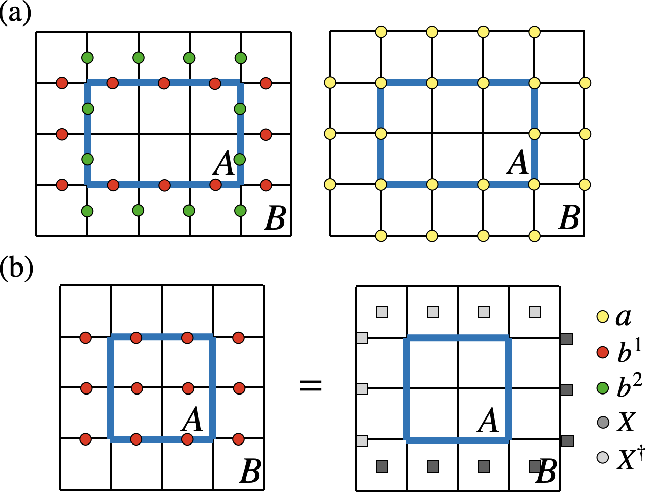
Figure 2: Region $A$ consists of spins on the blue boundary line and its interior. (a) Marginal stabilizers among $b_{i}^{x}$, $b_{i}^{y}$’s (left) and $a_{i}$’s (right) having support in both $A$ and $B$ regions are indicated as colored circles. (b) Product of stabilizers in the region $A$ (left) is equal to the product of $X$ (and $X^{\dagger}$) operators along the boundary just outside of $A$ (right).

In further demonstration that the assignment $\gamma=3\log N$ is not arbitrary, we show that it is related to three boundary operators, defined as

$$\prod_{b_{i}^{x}\notin G_{B}}b^{x}_{i} \prod_{b_{i}^{y}\notin G_{B}}b^{y}_{i} \prod_{b_{i}^{x},b_{i}^{y}\notin G_{B}}(b^{x}_{i})^{-i_{y}}(b^{y}_{i})^{i_{x}}.$$ , , (6)

In each case, we have the product of $b$’s with $i\notin G_{B}$ meaning that the corresponding stabilizer at $i=(i_{x},i_{y})$ is not fully supported in region $B$. This includes stabilizers fully supported in $A$, and some marginal stabilizers as shown in Fig. 2. Invoking explicit expressions of $b_{i}^{x},b_{i}^{y}$ in terms of $X$ (see Fig. 1 and si ), one finds that all the $X$-operators in the interior of $A$ cancel out for the three products in (6), leaving only the product of $X$’s and $X^{\dagger}$’s along the boundary $\partial A$ as illustated in Fig. 2 (b). Formally, the three boundary operators in (6) provide three additional elements to $G_{B}$ that are not made up of $b_{i}$ stabilizers lying entirely in the region $B$. As a result, $|G_{B}|$ is larger by $N^{3}$ than the cardinality without such contributions, and give rise to $\gamma=3\log N$ in TEE. To further check the validity of our results, we followed the TEE extraction strategy prescribed in Kitaev and Preskill (2006) and found $\gamma=3\log N$.

So far we have left out the $W$’s as generators of $G$. When they are included in $G$, one can without loss of generality choose to place them entirely in the region $B$ but not in $A$. This changes the cardinality of both $G$ and $G_{B}$ but not of $G_{A}$, in such a way that the ratio $|G|/|G_{B}|$ and hence the TEE remains unchanged si . The argument fails for the non-contractible boundary since some of the WW operators must cross the boundary no matter how they are deformed. The state constructed in (3) is only one of the possible ground states, but one can show that all other ground states share the same TEE as long as the boundary is contractible si .

We now consider a pair of parallel and non-contractible boundaries along the $x$- or $y$-axis of the torus and call them $x$-cut and $y$-cut, respectively. For non-contractible boundaries, a particular combination of the ground states called the minimum entropy states (MESs), constructed as a simultaneous eigenstate of all logical operators running along the cut, plays a significant role in the consideration of TEE Dong et al. (2008); Zhang et al. (2012). In general, the eigenvalue of any given logical operator is an integer power mod $N$ of $\omega$. It can be shown that in the R2TC, MESs with different eigenvalues of logical operators yield the same TEE si . It thus suffices to construct the MES with eigenvalue +1 for all the corresponding logical operators, by generating the group $G$ using $b_{i}^{1},b_{i}^{2}$, and $W_{1},W_{3},W_{5}$ defined along the $x$-axis. (WW operators defined along the $y$-axis are $W_{2},W_{4},W_{6}$.)

Now we are ready to construct a MES for the $x$-cut as

$$\ket{\psi_{\rm MES}}=|G_{\rm MES}|^{-1/2}\sum_{g\in G_{\rm MES}}g\ket{0},$$ (7)

with the group $G_{\rm MES}$ generated by $b_{i}^{x}$, $b_{i}^{y}$, and $W_{1}$,$W_{3}$,$W_{5}$. First of all, note that a state in (7) is automatically an eigenstate of $g\in G_{\rm MES}$ with eigenvalue +1 and thus of $W_{1}$,$W_{3}$,$W_{5}$. It is also an eigenstate of all $\widetilde{W}$’s running along the $x$-axis, with eigenvalue +1, as they commute with ($W_{1}$,$W_{3}$,$W_{5}$) si . Therefore, $|\psi_{\rm MES}\rangle$ constructed in (7) is a MES for arbitrary $L_{x}\times L_{y}$. The entanglement entropy of such MES can be obtained si , $S_{\rm MES}^{x}=4L_{x}\log N-\gamma^{x}_{\rm MES}$, with

$$\gamma^{x}_{\rm MES}=\log(N^{4}\gcd(L_{x},N)^{2}).$$ (8)

A similar construction of MES for the $y$-cut uses ($W_{2}$,$W_{4}$,$W_{6}$) as generators and gives

$$\gamma^{y}_{\rm MES}=\log(N^{4}\gcd(L_{y},N)^{2}).$$ (9)

We have successfully confirmed that the system size dependence not only exists in GSD Oh et al. (2022a); Pace and Wen (2022) but also in TEE for the bi-partition by non-contractible loops. Having explicit formulas for both TEE in (8)-(9) and GSD in (2), we now look for a theoretical framework to understand them.

The $\mathbb{Z}_{N}$ R2TC has translation symmetry in both the $x$ and $y$ directions. However, acting on an anyon with translation symmetry will, in general, change the anyon type as demonstrated by (1). For example, an anyon with $l_{1}=1$ and all other $l_{i}=0$ on the site $(0,0)$ transforms under translation symmetry $T_{x}$ to an anyon with $l_{1}=1$ but $l_{2}=-1$ on site $(1,0)$, and is therefore topologically distinct from the original anyon. It also follows from (1) that both $T_{x}$ and $T_{y}$ generate anyon permutations of rank $N$, that is, $T_{x}^{N}$ and $T_{y}^{N}$ leave the anyon type unchanged. If we coarse-grain to an $N\times N$ unit cell, then we can roughly think of the system as having an “on-site” symmetry group $\mathrm{G}=\mathbb{Z}^{(x)}_{N}\times\mathbb{Z}^{(y)}_{N}$ (the superscript notation is just a reminder that $T_{x}$ generates the first copy of $\mathbb{Z}_{N}$ and $T_{y}$ the second). Although the symmetry is not actually on-site, we will treat it as such in what follows according to the crystalline equivalence principle Thorngren and Else (2018). In this view, the R2TC should be viewed as a $\mathbb{Z}_{N}\times\mathbb{Z}_{N}$ SET.

In this coarse-grained view, choosing a linear system size $L_{x}$ such that $N$ does not divide $L_{x}$ introduces a symmetry defect piercing the $x$ handle of the torus. This means that, if we define

$$L_{x}~{}{\rm mod}~{}N\equiv m,~{}~{}L_{y}~{}{\rm mod}~{}N\equiv n,$$ (10)

any excitation traversing the $x$ handle of the torus will be acted upon by the element ${\bf g}=m$ of $\mathbb{Z}^{(x)}_{N}$ (in additive notation). Similarly, $L_{y}$ not divisible by $N$ gives rise to another symmetry defect ${\bf h}=n$ of $\mathbb{Z}^{(y)}_{N}$ piercing the $y$ handle of the torus. Any excitation that traverses the $y$ handle of the torus will be acted on by ${\bf h}$.

It is well-understood how to characterize symmetry defects in the presence of anyons; the correct mathematical framework is a “$\mathrm{G}$-crossed modular tensor category.”  Barkeshli et al. (2019); Tarantino et al. (2016); Turaev (2000); Etingof et al. (2010) (To avoid confusion with the notation $G$ for the group of generators earlier, we use the roman G when referring to symmetry defects.) We briefly summarize the salient results of Barkeshli et al. (2019). Given a $\mathrm{G}$-enriched topological phase, there are many symmetry defects associated to a group element ${\bf g}\in\mathrm{G}$; we call the set of such defects ${\cal C}_{\bf g}$. We denote one such defect as $a_{\bf g}$. (If ${\bf 0}$ is the identity element of $\mathrm{G}$, then the set of ${\bf 0}$ defects is just the anyons of the theory.) Any one of the defects associated to ${\bf g}$ can be obtained from any other by fusing it with some anyon.

Each symmetry defect $a_{\bf g}$ has essentially the same properties as an anyon, including all the data associated with fusion and braiding. The main difference is that if one defect braids around another, it can change defect type because it is acted upon by an element of the symmetry group. In particular, if $a_{\bf g}$ does a full braid with $b_{\bf h}$ $({\bf h}\in\mathrm{G})$, then we say that $a_{\bf g}$ transforms as $a_{\bf g}\rightarrow\,^{\bf h}a_{\bf g}$. If it turns out that $\,{}^{\bf h}a_{\bf g}=a_{\bf g}$, that is, the defect type does not change under the action of ${\bf h}$, then we say that $a_{\bf g}$ is ${\bf h}$-invariant. We denote the set of ${\bf h}$-invariant ${\bf g}$ defects by $\mathcal{C}_{\bf g}^{\bf h}$.

The number of distinct ${\bf g}$ defects (denoted $|{\cal C}_{\bf g}|$) is

$$|{\cal C}_{\bf g}|=|{\cal C}_{\bf 0}^{\bf g}|=\text{\# of }{\bf g}\!\!-\!\!\text{invariant anyons}.$$ (11)

It is straightforward to show that if all the anyons are Abelian, then all ${\bf g}$ defects have the same quantum dimension. Using the fact that the total quantum dimension of the ${\bf g}$ defects must equal the total quantum dimension of the anyons, it follows that the quantum dimension $d_{a_{\bf g}}$ of any ${\bf g}$ defect is

$$d_{a_{\bf g}}=\sqrt{\frac{\text{\# of anyons}}{\text{\# of }{\bf g}\!\!-\!\!\text{invariant anyons}}}.$$ (12)

For the contractible boundary, TEE of a state with a quasiparticle $a$ inside the region $A$ is Dong et al. (2008); Kitaev and Preskill (2006)

$$\gamma=\log\frac{\cal D}{d_{a}}.$$ (13)

In the ground state for $L_{x},L_{y}$ divisible by $N$, there are no quasiparticle inside $A$ (other than the vacuum itself) and $\gamma=\log{\cal D}=3\log N$. An arbitrary $L_{x},L_{y}$ means that defects $\bf{g}$ and $\bf{h}$ are piercing the $x$ and $y$ handles of the torus, respectively. Therefore, still only the vacuum is inside $A$, which means $\gamma=3\log N$, in agreement with our earlier result, (5). We see that the defect picture gives a consistent interpretation of the lack of system size dependence in the case of contractible boundary.

In the absence of symmetry defects, the entanglement entropy of a MES on the torus associated to an anyon $a_{\bf 0}$ threading the $x$-cut cycle is given by Dong et al. (2008); Zhang et al. (2012)

$$\gamma_{\rm MES}^{(a_{\bf 0})}=2\log\frac{\mathcal{D}}{d_{a_{\bf 0}}}.$$ (14)

We assume that the analogous formula holds in twisted sectors, i.e., when a symmetry defect $a_{\bf g}$ threads the $x$-cut cycle instead:

$$\gamma_{\rm MES}^{(a_{\bf g})}=2\log\frac{\mathcal{D}}{d_{a_{\bf g}}}.$$ (15)

Ref. Chen et al. (2022) found that various other TEE formulas involving only anyons, such as Eq. (13), can be directly generalized to the defect case in the same way, which justifies our assumption. When all the anyons are Abelian, $\mathcal{D}^{2}$ is just the total number of anyons, so we find

$$\gamma_{\rm MES}^{(a_{\bf g})}=\log\left(\text{\# of }{\bf g}\!\!-\!\!\text{invariant anyons}\right)$$ (16)

One can explicitly show that indeed, the number of ${\bf g}$-invariant anyons in the R2TC is $N^{4}\gcd(L_{x},N)^{2}$ si , in agreement with $\gamma_{\rm MES}^{x}$ in (8). A similar reasoning of $\gamma_{{\rm MES}}^{(a_{\bf h})}$ correctly captures $\gamma_{\rm MES}^{y}$ in (9).

We conclude that the system size dependence of the TEE can be adequately explained by thinking of the system as a coarse-grained system enriched by a $\mathbb{Z}_{N}\times\mathbb{Z}_{N}$ symmetry arising from microscopic translations.

Likewise, the torus GSD can be explained in the same language. G-crossed modularity Barkeshli et al. (2019) requires that

$$\text{GSD}({\bf g,h}) =\text{\# of }{\bf g}\!-\!\text{invariant }{\bf h}\text{ defects}$$

$$=\text{\# of }{\bf h}\!-\!\text{invariant }{\bf g}\text{ defects}$$ (17)

(Unlike our TEE formula, this formula has been proven rigorously.) For ${\bf g}=0$, this is just the number of ${\bf h}$ defects, which, as already stated, is $N^{4}\gcd(L_{y},N)^{2}$, with an analogous formula when the roles of $L_{x}$ and $L_{y}$ swap. We carefully show in the SI si that the general formula is si

$$\text{\# of }{\bf g}\!-\!\text{invariant }{\bf h}\text{ defects}$$

$$=N^{3}\gcd(L_{x},N)\gcd(L_{y},N)\gcd(L_{x},L_{y},N)$$ (18)

which matches the GSD formula in (2).

We have demonstrated that both the TEE and GSD of the R2TC can be comprehensively understood by conceptualizing it as a translation SET and using the symmetry defect theory.

A few additional remarks are in order. One can use the tensor network ground state wave function for R2TC proposed in Oh et al. (2023) to compute the entanglement entropy numerically. Due to severe computational costs, it turns out the calculation is currently limited to $N=2$ and $L_{y}\leq 3$ for the case of the $y$-cut, with $L_{x}\leq 5$. Following the procedure outlined in Cirac et al. (2011); Oh et al. (2023); si , we numerically find the entanglement entropy in excellent agreement with $S^{y}_{\rm MES}=4L_{y}\log N-\log(N^{4}{\rm gcd}(L_{y},N)^{2})$ for $N=2$, $L_{y}=3$ and $L_{x}=4,5$, confirming the validity of our derivation. Secondly, it is known that spurious TEE can appear for some non-topological states Zou and Haah (2016); Williamson et al. (2019); Watanabe et al. (2023). To check that our results are not being plagued by such effects, we use the model proposed in Williamson et al. (2019) and construct bulk products similar to (6). After the interior terms again cancel out, leaving the product of operators along the boundary of $A$. Importantly, this product does not completely encircle the boundary, as is the case in R2TC and other topological models, but is limited to a finite segment. Consequently, the TEE depends on the shape of the boundary and the area of the region (see Fig. S3). With this observation, we can ensure that the TEE of R2TC is a genuine TEE. This comprehension can serve as a useful diagnostic for distinguishing between spurious and genuine TEE.

In conclusion, we have performed systematic calculations of TEE for the rank-2 toric code and found system size dependence similar to the system size dependence of the GSD. We quantitatively explain the TEE by viewing the R2TC as a translation SET with symmetry defects threaded through non-contractible cycles of the torus. Our work shows that the symmetry defect picture is powerful enough to straightforwardly predict topological properties beyond the GSD while not requiring a distinction between local and global equivalence of excitation configurations. Given the wide range of unique features in such translation SETs, it would be highly interesting to realize such models in spin, Rydberg atom, or other synthetic systems. It may also be possible to use our understanding of such translation SETs in (2+1) dimensions as a stepping stone to a more general understanding of (3+1)-dimensional phases with system size-dependent GSDs, including translation SETs and fracton topological orders.

Acknowledgments.

- We are grateful to Isaac Kim for helpful discussions and feedback, and to Yizhi You for an earlier collaboration. Y.-T. O. acknowledges support from the National Research Foundation of Korea (NRF), funded by the Korean government (MSIT), under grants No. RS-2023-00220471 and NRF-2022R1I1A1A01065149, as well as from the Basic Science Research Program funded by the Ministry of Education under grant 2014R1A6A1030732. D.B. was supported for part of this work by the Simons Collaboration on Ultra-Quantum Matter, which is a grant from the Simons Foundation (No. 651440). J.H.H. was supported by the National Research Foundation of Korea(NRF) grant funded by the Korea government(MSIT) (No. 2023R1A2C1002644). He acknowledges KITP, supported in part by the National Science Foundation under Grant No. NSF PHY-1748958, where this work was finalized.

I Entanglement Entropy Formula

In this section, we summarize a derivation of the entanglement entropy expression presented in (4) Hamma et al. (2005); Ebisu (2023b). The entanglement entropy $S_{A}$ associated with the region $A$ is formally defined as

$$S_{A}=\lim_{n\rightarrow 1}\frac{1}{1-n}\log\mathrm{Tr}[\rho_{A}^{n}],$$ (S1)

where $\rho_{A}={\rm Tr_{B}}[\rho]$ is the reduced density matrix for region $A$. $S_{A}$ is also recognized as the Renyi entanglement entropy. Starting from the pure state expression in (3), $\rho_{A}$ can be expressed as

$$\rho_{A} ={\rm Tr}_{B}[\ket{\psi}\bra{\psi}]$$

$$=|G|^{-1}{\rm Tr}_{B}[\sum_{g\in G,g^{\prime}\in G}g\ket{0}\bra{0}(gg^{\prime})^{{\dagger}}]$$

$$=|G|^{-1}{\rm Tr}_{B}[\sum_{g\in G,g^{\prime}\in G}g_{A}\ket{0}_{A}\bra{0}_{A}(g_{A}g_{A}^{\prime})^{{\dagger}}\otimes g_{B}\ket{0}_{B}\bra{0}_{B}(g_{B}g_{B}^{\prime})^{{\dagger}}]$$

$$=|G|^{-1}\sum_{i,j,g\in G,g^{\prime}\in G}g_{A}\ket{0}_{A}\bra{0}_{A}(g_{A}g_{A}^{\prime})^{{\dagger}}\otimes\bra{0}_{B}(g_{B}g_{B}^{\prime})^{{\dagger}}g_{B}\ket{0}_{B},$$ (S2)

where $g=g_{A}\otimes g_{B}$ and $\ket{0}=\ket{0}_{A}\otimes\ket{0}_{B}$. The requisite condition for the non-vanishing of $\bra{0}_{B}(g_{B}g_{B}^{\prime})^{\dagger}g_{B}\ket{0}B$ is $g_{B}^{\prime}=I_{B}$. Subsequently, the formulation for $\rho_{A}$ adopts the structure

$$\rho_{A}=|G|^{-1}\sum_{g\in G,g^{\prime}\in G_{A}}g_{A}\ket{0}_{A}\bra{0}A(g_{A}g_{A}^{\prime})^{\dagger},$$ (S3)

where $G_{A}=\{g\in G|g=g_{A}\otimes I_{B}\}$. Employing (S3), we proceed to deduce $\rho_{A}^{2}=|G_{A}||G_{B}|/|G|\rho_{A}$ Hamma et al. (2005); Ebisu (2023b). After all, we arrive at

$$S_{A} =\lim_{n\rightarrow 1}\frac{1}{1-n}\log\mathrm{Tr}\left[\left(\frac{|G_{A}||G_{B}|}{|G|}\right)^{n-1}\rho_{A}\right]$$

$$=\log\left(\frac{|G|}{|G_{A}|\cdot|G_{B}|}\right)$$ (S4)

as the conclusive expression.

II stabilizer identities in R2TC

In the rank-2 toric code (R2TC), there are three stabilizers $a_{i}$, $b_{i}^{x}$, and $b_{i}^{y}$ associated with sites $i$, links $(i,i+\hat{x})$, and $(i,i+\hat{y})$ on a square lattice, respectively. They correspond to one electric and two magnetic excitations as:

$$a_{i} =Z_{0,i}Z_{0,i-\hat{x}}^{-1}Z_{0,i-\hat{y}}^{-1}Z_{0,i-\hat{x}-\hat{y}}Z_{2,i-\hat{y}}Z_{2,i}^{-2}Z_{2,i+\hat{y}}Z_{1,i-\hat{x}}Z_{1,i}^{-2}Z_{1,i+\hat{x}}$$

$$b_{i}^{x} =X_{2,i}^{1}X_{2,i+\hat{x}}^{-1}X_{0,i}X_{0,i-\hat{y}}^{-1}$$

$$b_{i}^{y} =X_{1,i}X_{1,i+\hat{y}}^{-1}X_{0,i}X_{0,i-\hat{x}}^{-1}.$$ (S5)

We label the sites by $i=(i_{x},i_{y})$. $\mathbb{Z}_{N}$ Pauli-$X,Z$ operators are defined by their actions $(\omega=e^{2\pi i/N})$:

$$X_{a,i}|g\rangle_{a,i}=|g+1~{}({\rm mod}~{}N)\rangle_{a,i},~{}~{}Z_{a,i}|g\rangle=\omega^{g}|g\rangle_{a,i}.$$ (S6)

Operators with subscript 0 are defined at the center of the plaquette associated with the site $i$ while those with subscripts $1$, $2$ are both defined at the site as illustrated in Fig. 1.

We summarize several identities held by stabilizers and logical operators of R2TC that will prove to be of use in the evaluation of TEE. Three of them come directly from the definition of stabilizers:

$$I_{1} \equiv\prod_{i}a_{i}=1~{}~{}~{}~{}~{}~{}~{}I_{2}\equiv\prod_{i}b_{i}^{x}=1~{}~{}~{}~{}~{}~{}~{}I_{3}\equiv\prod_{i}b_{i}^{y}=1.$$ (S7)

The product $\prod_{i}$ runs over all the sites of the square lattice forming a torus, $1\leq i_{x}\leq L_{x},~{}1\leq i_{y}\leq L_{y}$. Heuristically, they imply the conservation of the total electric ($I_{1}$) and two magnetic ($I_{2},I_{3}$) charges mod $\mathbb{Z}_{N}$. The other three identities are

$$I_{4} \equiv\left[\prod_{i}(a_{i})^{i_{x}}\right]^{c_{x}}=1,$$

$$I_{5} \equiv\left[\prod_{i}(a_{i})^{i_{y}}\right]^{c_{y}}=1,$$

$$I_{6} \equiv\left[\prod_{i}(b^{x}_{i})^{-i_{y}}(b^{y}_{i})^{i_{x}}\right]^{c_{xy}}=1.$$ (S8)

Each stabilizer is raised to a power of the coordinate, and the identities $I_{4}$, $I_{5}$, $I_{6}$ refer to the conservation of electric dipoles in the $x$ direction, electric dipoles in the $y$ direction, and magnetic angular momentum, respectively. Importantly, the identities are obtained when the products are raised to appropriate “winding numbers” $c_{x},~{}c_{y},~{}c_{xy}$ given by

$$c_{x} =N/{\rm gcd}(L_{x},N)={\rm lcm}(L_{x},N)/L_{x},$$

$$c_{y} =N/{\rm gcd}(L_{y},N)={\rm lcm}(L_{y},N)/L_{y},$$

$$c_{xy} =N/{\rm gcd}(L_{x},L_{y},N).$$ (S9)

The necessity to introduce them becomes clear when we evaluate

$$\prod_{i}(a_{i})^{i_{x}} =\prod_{i_{y}}Z_{1,\hat{x}+i_{y}\hat{y}}^{L_{x}}Z_{1,L_{x}\hat{x}+i_{y}\hat{y}}^{-L_{x}}$$

$$\prod_{i}(a_{i})^{i_{y}} =\prod_{i_{x}}Z_{2,i_{x}\hat{x}+\hat{y}}^{L_{y}}Z_{2,i_{x}\hat{x}+L_{y}\hat{y}}^{-L_{y}}$$

$$\prod_{i}(b^{x}_{i})^{-i_{y}}(b^{y}_{i})^{i_{x}} =\prod_{i_{y}}X_{0,L_{x}\hat{x}+i_{y}\hat{y}}^{L_{x}}\prod_{i_{x}}X_{0,i_{x}\hat{x}+L_{y}\hat{y}}^{-L_{y}}.$$ (S10)

In general they are not equal to an identity unless $L_{x},L_{y}$ are multiples of $N$. To guarantee their identity we need to find the smallest positive integers $n_{x}$, $n_{y}$, and $n_{xy}$ satisfying

$$L_{x}n_{x}~{}{\rm mod}~{}N=0,~{}~{}L_{y}n_{y}~{}{\rm mod}~{}N=0$$

$$L_{x}n_{xy}~{}{\rm mod}~{}N=0~{}~{}\&~{}~{}L_{y}n_{xy}~{}{\rm mod}~{}N=0.$$ (S11)

The first two relations give $n_{x}=c_{x}$ and $n_{y}=c_{y}$. For $n_{xy}$,

$$n_{xy}={\rm lcm}\left(\frac{N}{{\rm gcd}(L_{x},N)},\frac{N}{{\rm gcd}(L_{y},N)}\right)=\frac{N}{{\rm gcd}({\rm gcd}(L_{x},N),{\rm gcd}(L_{y},N))}=\frac{N}{{\rm gcd}(L_{x},L_{y},N)}=c_{xy}.$$ (S12)

We refer to the six identities $I_{1}$ through $I_{6}$ as the “stabilizer identities” of the R2TC.

The six stabilizer identities derived above can be used to evaluate the ground state degeneracy (GSD), by comparing the number of identities against the total number of stabilizers in the model. This approach, already used in Kitaev’s toric code paper Kitaev (2003), was applied for the initial GSD calculation of $\mathbb{Z}_{N}$ R2TC Oh et al. (2022a) assuming $N$ is a prime number. We now have relaxed this condition and obtained identities (S7) and (S8) that hold for arbitrary integer $N$. Each of the three identities $I_{1},I_{2},I_{3}$ generates $N$ constraint for the stabilizers since $(I_{1})^{n_{1}}=(I_{2})^{n_{2}}=(I_{3})^{n_{3}}=1$ for $1\leq n_{1},n_{2},n_{3}\leq N$. The GSD becomes $N\times N\times N=N^{3}$. From the three remaining identities we have $(I_{\alpha})^{n_{\alpha}}=1$ with $1\leq n_{4}\leq{\rm gcd}(L_{x},N)$, $1\leq n_{5}\leq{\rm gcd}(L_{y},N)$, and $1\leq n_{6}\leq{\rm gcd}(L_{x},L_{y},N)$, respectively. The full GSD formula of (2) is recovered in this simple manner.

Among the six identities, $\{I_{2},I_{3},I_{6}\}$ come from taking the product of magnetic stabilizers and the remaining $\{I_{1},I_{4},I_{5}\}$ from those of electric stabilizers. The fact that there are three identities for each type of stabilizers plays a crucial role in the evaluation of TEE.

III WW operators in $X$-operator basis

There are six Wegner-Wilson (WW) operators, which are products of $X$’s. These operators correspond to the movement of electric monopoles and dipoles along the non-contractible loops of the torus Oh et al. (2023):

$$W_{1,i_{y}} =\prod_{i_{x}=1}^{L_{x}}X_{0,i},~{}~{}~{}~{}~{}~{}~{}~{}~{}~{}~{}~{}~{}W_{2,i_{x}}=\prod_{i_{y}=1}^{L_{y}}X_{2,i},~{}~{}~{}~{}~{}~{}~{}~{}~{}~{}~{}~{}~{}W_{3,i_{y}}=\prod_{i_{x}=1}^{L_{x}}X_{1,i},~{}~{}~{}~{}~{}~{}~{}~{}~{}~{}~{}~{}~{}W_{4,i_{x}}=\prod_{i_{y}=1}^{L_{y}}X_{0,i}$$

$$W_{5,i_{y}} =\prod_{i_{x}=1}^{{\rm lcm}(L_{x},N)}(X_{1,i})^{i_{x}}(X_{0,i})^{i_{y}},~{}~{}~{}~{}~{}~{}~{}~{}~{}~{}~{}~{}~{}~{}~{}~{}~{}~{}~{}~{}~{}~{}~{}~{}~{}~{}~{}~{}~{}~{}W_{6,i_{x}}=\prod_{i_{y}=1}^{{\rm lcm}(L_{y},N)}(X_{2,i})^{i_{y}}(X_{0,i})^{i_{x}}.$$ (S13)

In some cases, $i_{x}$ and $i_{y}$ can be omitted for simplicity. An arbitrary WW operator $W_{a,i_{x}^{\prime}(i_{y}^{\prime})}$ can be expressed as the product of WW operators in Eq. (S13) and the stabilizers $b_{i}^{x}$ and $b_{i}^{y}$.

The WW operators can be used to account for the GSD. Among the six WW operators, $W_{2}$ and $W_{3}$ satisfy $(W_{2})^{N}=(W_{3})^{N}=1$, each giving a factor $N$ for the number of independent logical operators and therefore the distinct ground states. With $W_{5}$ and $W_{6}$ the degeneracy count is not as simple, since we do not have $(W_{5})^{\gcd(L_{x},N)}$ and $(W_{6})^{\gcd(L_{y},N)}$ equal to unity in general. Instead, we can show that $W_{5}$ and $W_{6}$ can be re-organized as

$$W_{5} =\prod_{i_{x}=1}^{L_{x}}X_{1,i}^{\frac{{\rm lcm}(L_{x},N)}{2L_{x}}\left(\frac{{\rm lcm}(L_{x},N)}{L_{x}}-1\right)+\frac{{\rm lcm}(L_{x},N)}{L_{x}}i_{x}}X_{0,i}^{\frac{{\rm lcm}(L_{x},N)}{L_{x}}i_{y}}$$

$$W_{6} =\prod_{i_{y}=1}^{L_{y}}X_{2,i}^{\frac{{\rm lcm}(L_{y},N)}{2L_{y}}\left(\frac{{\rm lcm}(L_{y},N)}{L_{y}}-1\right)+\frac{{\rm lcm}(L_{y},N)}{L_{y}}i_{y}}X_{0,i}^{\frac{{\rm lcm}(L_{y},N)}{L_{y}}i_{x}},$$ (S14)

since the exponents of the $X_{1,i}$, $X_{2,i}$ are $\sum_{j}(j*L_{x}+i_{x})$ while the one of the $X_{0,i}$ is $\sum_{j}i_{x}$. Therefore,

$$(W_{5})^{{\rm gcd}(L_{x},N)} =\prod_{i_{x}=1}^{L_{x}}X_{1,i}^{\frac{N}{2}\left(\frac{{\rm lcm}(L_{x},N)}{L_{x}}-1\right)}=(W_{3})^{\frac{N}{2}\left(\frac{{\rm lcm}(L_{x},N)}{L_{x}}-1\right)}$$

$$(W_{6})^{{\rm gcd}(L_{y},N)} =\prod_{i_{y}=1}^{L_{y}}X_{2,i}^{\frac{N}{2}\left(\frac{{\rm lcm}(L_{y},N)}{L_{y}}-1\right)}=(W_{2})^{\frac{N}{2}\left(\frac{{\rm lcm}(L_{y},N)}{L_{y}}-1\right)},$$ (S15)

both of which are equal to some powers of existing logical operators. Although intuitively clear, one can prove that the two exponents appearing on the r.h.s. are indeed integers. First for $N$ even, the exponents appearing at the far right are obviously integers. For odd $N$, one can show that ${\rm lcm}(L_{x},N)/L_{x}$ is an odd integer, and the exponent is again an integer. (The proof is elementary. When ${\rm lcm}(L_{x},N)$ and $L_{x}$ are factorized in terms of prime numbers, both factorizations must contain the same number of 2’s in them because $N$ is odd. Hence, the ratio ${\rm lcm}(L_{x},N)/L_{x}$ must be expressed as a product of odd prime numbers and become an odd number.) To conclude, $(W_{5})^{{\rm gcd}(L_{x},N)}$ and $(W_{6})^{{\rm gcd}(L_{y},N)}$ are some integer multiples of existing logical operators $W_{2}$ and $W_{3}$ and no longer independent logical operators.

Finally we come to $W_{1},W_{4}$, both of which are products of $X_{0}$’s. As the combination $W_{1}^{n_{1}}W_{4}^{n_{4}}$ with various equivalence relations

$$(n_{1},n_{4})\equiv(n_{1}+N_{y},n_{4})\equiv(n_{1},n_{4}+N_{x})\equiv(n_{1}+L_{y},n_{4}-L_{x})$$ (S16)

where $N_{x}=\gcd(c_{y}L_{x},N)$, $N_{y}=\gcd(c_{x}L_{y},N)$ Oh et al. (2023). We need to check how many inequivalent integers $(n_{1},n_{4})$ are allowed under the equivalence relations. Due to the first two relations in (S16), we conclude $1\leq n_{1}\leq N_{y}$ and $1\leq n_{4}\leq N_{x}$. Furthermore, the number of different integer expressions $(n_{1},n_{4})$ that become equivalent due to $(n_{1},n_{4})\equiv(n_{1}+L_{y},n_{4}-L_{x})$ is

$${\rm lcm}\Bigl{(}\frac{{\rm lcm}(L_{x},N_{x})}{L_{x}},\frac{{\rm lcm}(L_{y},N_{y})}{L_{y}}\Bigl{)}.$$ (S17)

Therefore the total number of independent products of $W_{1}$ and $W_{4}$ is

$$\frac{N_{x}N_{y}}{{\rm lcm}\Bigl{(}\frac{{\rm lcm}(L_{x},N_{x})}{L_{x}},\frac{{\rm lcm}(L_{y},N_{y})}{L_{y}}\Bigl{)}} ={\rm gcd}\Bigl{(}N_{y}\gcd(L_{x},N_{x}),N_{x}\gcd(L_{y},N_{y})\Bigl{)}$$

$$=N{\rm gcd}\Bigl{(}\gcd(L_{x},N),\gcd(L_{y},N)\Bigl{)}$$

$$=N{\rm gcd}(L_{x},L_{y},N).$$ (S18)

To conclude, we have degeneracy factors of $N$ from $W_{2}$ and $W_{3}$ each, $\gcd(L_{x},N)$ and $\gcd(L_{y},N)$ from $W_{5}$ and $W_{6}$ each, and the factor of $N{\rm gcd}(L_{x},L_{y},N)$ from the combination of $W_{1}$ and $W_{4}$ for a total of $N^{3}{\rm gcd}(L_{x},N){\rm gcd}(L_{y},N){\rm gcd}(L_{x},L_{y},N)$ independent logical operators.

For the last, we determine how many WW operators are defined along the $x$-axis or $y$-axis to construct the MES. We can be sure that $W_{3}$ and $W_{5}$ are defined along $x$-axis, and $W_{2}$ and $W_{6}$ are defined along $y$-axis. However, it is tricky to count the numbers of $W_{1}$ and $W_{4}$ because of equivalence relations in Eq. (S16). When $N$ is a prime number, the following four cases can be observed: (1) both $L_{x}$ and $L_{y}$ are multiples of $N$, (2) only $L_{x}$ is a multiple of $N$, (3) only $L_{y}$ is a multiple of $N$, and (4) neither $L_{x}$ nor $L_{y}$ is a multiple of $N$. Within each of these cases, the corresponding outcomes are as follows: for case (1), both $W_{1}$ and $W_{4}$ are present; for case (2), only $W_{4}$ is present; for case (3), only $W_{1}$ is present; and for case (4), either $W_{1}$ or $W_{4}$ may exist, which means $W_{1}$ and $W_{4}$ become identical Oh et al. (2022a). The results are summarized in the Table 1.

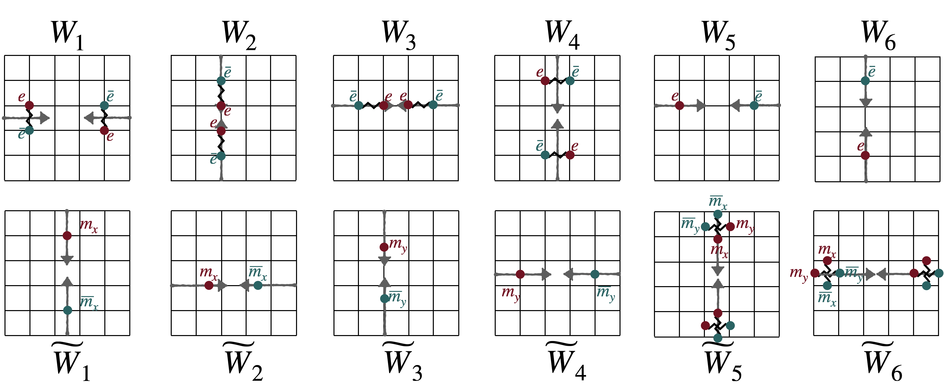
Figure S1: The CAPs associated with anyons and their corresponding anti-anyon pairs are illustrated for the respective WW operators.

	$L_{x}~{}{\rm mod}~{}N=0$	$L_{x}~{}{\rm mod}~{}N\neq 0$
$L_{y}~{}{\rm mod}~{}N=0$	($W_{1}$ $\widetilde{W}_{2}$ $W_{3}$ $\widetilde{W}_{4}$ $W_{5}$ $\widetilde{W}_{6}$)	($W_{1}$ $\widetilde{W}_{2}$ $W_{3}$ $\widetilde{W}_{6}$)
	$(\widetilde{W}_{1}$ $W_{2}$ $\widetilde{W}_{3}$ $W_{4}$ $\widetilde{W}_{5}$ $W_{6}$)	$(\widetilde{W}_{1}$ $W_{2}$ $\widetilde{W}_{3}$ $W_{6}$)
$L_{y}~{}{\rm mod}~{}N\neq 0$	($\widetilde{W}_{2}$ $W_{3}$ $\widetilde{W}_{4}$ $W_{5}$)	($\widetilde{W}_{2}$ $W_{3}$)
		($W_{[1\simeq 4]}$, $\widetilde{W}_{[1\simeq 4]}$)
	($W_{2}$ $\widetilde{W}_{3}$ $W_{4}$ $\widetilde{W}_{5}$)	($W_{2}$ $\widetilde{W}_{3}$)

Table 1: Classification of WW operators that function as logical operators. For each case, upper (lower) sets are the WW operators defined as products along the $x$- ($y$-)axis. We assume $N$ is a prime number. The middle row of the final entry ($L_{x},L_{y}~{}{\rm mod}~{}N\neq 0$) shows two WW operators $W_{[1\simeq 4]}$ and $\widetilde{W}_{[1\simeq 4]}$, which are neither extended along $x$ or $y$-direction.

IV WW operators in $Z$-operator basis

There are six WW operators in terms of $Z$’s:

$$\widetilde{W}_{1}= \prod_{i_{y}=1}^{{\rm lcm}(L_{y},N)}Z_{0,i-\hat{y}}\bigl{(}Z_{1,i}Z_{1,i+\hat{x}}^{-1}\bigr{)}^{i_{y}},~{}~{}~{}~{}~{}~{}~{}~{}~{}\widetilde{W}_{2}=\prod_{i_{x}=1}^{L_{x}}Z_{2,i}\bigl{(}Z_{2,i}Z_{2,i+\hat{y}}^{-1}\bigr{)}^{i_{y}},$$

$$\widetilde{W}_{3}= \prod_{i_{y}=1}^{L_{y}}Z_{1,i}\bigl{(}Z_{1}(\vec{v}_{i})Z_{1}(\vec{v}_{i}+\hat{x})^{-1}\bigr{)}^{i_{x}},~{}~{}~{}~{}~{}~{}~{}\widetilde{W}_{4}=\prod_{i_{x}=1}^{{\rm lcm}(L_{x},N)}Z_{0,i-\hat{x}}\bigl{(}Z_{2,i}Z_{2,i+\hat{y}}^{-1}\bigr{)}^{i_{x}},$$

$$\widetilde{W}_{5}= \prod_{i_{y}=1}^{L_{y}}Z_{1,i+\hat{x}}Z_{1,i}^{-1},~{}~{}~{}~{}~{}~{}~{}~{}~{}~{}~{}~{}~{}~{}~{}~{}~{}~{}~{}~{}~{}~{}~{}~{}~{}~{}~{}~{}~{}\widetilde{W}_{6}=\prod_{i_{x}=1}^{L_{x}}Z_{2,i+\hat{y}}Z_{2,i}^{-1}.$$ (S19)

Upon initial inspection, the contributions of each logical operator on GSD appear as $\gcd(L_{y},N)$, $N$, $N$, $\gcd(L_{x},N)$, $\gcd(L_{x},N)$, and $\gcd(L_{y},N)$. The collective result of these contributions yields a GSD computation of $N^{2}[\gcd(L_{x},N)\gcd(L_{y},N)]^{2}$, which under-span the ground state Hilbert space.

The deficiency of the ground state basis comes from the fact that $\widetilde{W}_{4}$ given in above expression is not the most minimal choice of the logical operator. The correct logical operator expression is given by Pace and Wen (2022); Oh et al. (2023)

$$\widetilde{W}_{4}^{\rm min}=\prod_{i_{x}=1}^{n_{x}L_{x}}Z_{0,i-\hat{x}}\bigl{(}Z_{2,i}Z_{2,i+\hat{y}}^{-1}\bigr{)}^{i_{x}}\prod_{i_{y}=1}^{n_{y}L_{y}}Z_{0,i-\hat{y}}\bigl{(}Z_{1,i}Z_{1,i+\hat{x}}^{-1}\bigr{)}^{i_{y}},$$ (S20)

where the integers $n_{x}$ and $n_{y}$ are given by

$$n_{x} =\frac{{\rm gcd}(L_{y},N)}{{\rm gcd}(L_{x},L_{y},N)}, n_{y} =\frac{{\rm lcm}\bigl{(}L_{x},{\rm gcd}(L_{y},N)\bigr{)}+kN}{L_{y}}.$$ (S21)

Here, $k$ is a minimal integer that makes $n_{y}$ an integer Pace and Wen (2022). The contribution of this logical operator corresponds to $N{\rm gcd}(L_{x},L_{y},N)/{\rm gcd}(L_{y},N)$. Substituting $\widetilde{W}_{4}$ in Eq. (S19) with $\widetilde{W}_{4}^{\rm min}$ yields the correct computation of GSD: $N^{3}{\rm gcd}(L_{x},N){\rm gcd}(L_{y},N){\rm gcd}(L_{x},L_{y},N)$.

The classification of six WW operators, which run along either the $x$-axis or the $y$-axis, can be easily done, except in situations where both $L_{x}$ and $L_{y}$ are not multiples of $N$. $\widetilde{W}_{2}$, $\widetilde{W}_{4}$, $\widetilde{W}_{6}$ are the product of $Z$’s along the $x$-axis and $\widetilde{W}_{1}$, $\widetilde{W}_{3}$, $\widetilde{W}_{5}$ are the product of $Z$’s along the $x$-axis. The results for the prime $N$ are summarized in the Table 1.

V Entanglement entropy: contractible boundary

The ground state we use for the calculation of entanglement entropy is $\ket{\psi}=|G|^{-1/2}\sum_{g\in G}g\ket{0}$, where $G$ is generated by two magnetic stabilizers $b_{i}^{x}$ and $b_{i}^{y}$. A naive estimate of $|G|$ for the group spanned by $(b_{i}^{x},b_{i}^{y})$ on a $L_{x}\times L_{y}$ lattice is $N^{2L_{x}L_{y}}$, ignoring the constraint among the stabilizers. As noted in previous section, there are three identities $I_{2}$, $I_{3}$, $I_{6}$ among the electric stabilizers that reduce the degree of freedom by factors of $N,N,{\rm gcd}(L_{x},L_{y},N)$, respectively, and therefore

$$|G|=N^{2L_{x}L_{y}}/(N^{2}\gcd(L_{x},L_{y},N)).$$ (S22)

We next compute $|G_{A}|$. We choose the region $A$ to be a $l_{x}\times l_{y}$ square as shown in Fig. S2. The spins lying on the boundary are counted as living inside $A$. (Such ambiguities exist in defining the entanglement boundary of the ordinary toric code as well and are not new.) The number of $b_{i}^{x}$’s and $b_{i}^{y}$’s acting entirely within the region $A$ is $N^{l_{x}(l_{y}-1)}$ and $N^{l_{y}(l_{x}-1)}$, respectively, and the cardinality of $G_{A}$ follows

$$|G_{A}|=N^{l_{x}(l_{y}-1)}\times N^{l_{y}(l_{x}-1)}=N^{l_{x}(l_{y}-1)+l_{y}(l_{x}-1)},$$ (S23)

before considering the constraints among the stabilizers through the three identities $I_{2}=I_{3}=I_{6}=1$ defined throughout in Eqs. (S7) and (S8). Without loss of generality, however, we may pretend the non-independent stabilizers are living entirely in the region $B$ and $|G_{A}|$ evaluated in (S23) is valid.

Now we come to the cardinality $|G_{B}|$. Ignoring the constraint among the stabilizers for the moment, counting the number of $b_{i}^{x},b_{i}^{y}$ stabilizers such that $b_{i}^{x}\notin G_{B}$ and $b_{i}^{y}\notin G_{B}$ ($\notin$ means the stabilizer does not lie entirely within $B$, encompassing even those that are defined exclusively in set $A$.) gives $(l_{x}+1)(l_{y}+2)$ and $(l_{x}+2)(l_{y}+1)$, respectively, leading to the naive count $|G^{\prime}_{B}|=|G|/N^{(l_{x}+1)(l_{y}+2)+(l_{x}+2)(l_{y}+1)}$. Note that in some cases an individual stabilizer does not lie fully inside $B$ but their product does, and qualifies as an element of $G_{B}$. Explicitly, they are

$$\prod_{b_{i}^{x}\notin G_{B}}b^{x}_{i} \prod_{b_{i}^{y}\notin G_{B}}b^{y}_{i} \prod_{b_{i}^{x},b_{i}^{y}\notin G_{B}}(b^{x}_{i})^{-i_{y}}(b^{y}_{i})^{i_{x}}.$$ (S24)

Each product spans all the sites $i$ for which the corresponding stabilizer does not lie fully inside the region $B$. One can readily check that the $X$ operators in the interior cancel out, leaving only the product of $X$’s and $X^{\dagger}$’s along the one-dimensional loop closely following the boundary of $A$. Importantly, all the $X$ operators that survive are located in the region $B$, and thus the three products in (S24) are indeed elements of $G_{B}$. The correct cardinality of $G_{B}$ is greater than $|G^{\prime}_{B}|$ evaluated above, and equals

$$|G_{B}|=|G^{\prime}_{B}|\times N^{3}=|G|N^{3-(l_{x}+1)(l_{y}+2)-(l_{y}+1)(l_{x}+2)}.$$ (S25)

Combining the results of $|G|,|G_{A}|,|G_{B}|$ we arrive at the entanglement entropy of a disk-like bi-partition:

$$S_{A}=\log(|G|/(|G_{A}||G_{B}|))=[4(l_{x}+l_{y}+1)-3]\log N.$$ (S26)

The same calculation for the regular toric code gives $S_{A}=[2(l_{x}+l_{y})-1]\log N$, where $2(l_{x}+l_{y})$ is interpreted as the length of the boundary and $\log N$ is the TEE. By comparison, the rank-2 calculation gives twice the geometric length, and an extra factor +1, with the TEE equal to $3\log N$. We claim that a satisfactory interpretation of the factor $4(l_{x}+l_{y}+1)$ is as the number of $b_{i}^{x}$ and $b_{i}^{y}$’s that do not belong wholly to $G_{A}$ or $G_{B}$, or marginal stabilizers. The extra factor 2 comes from having two types of stabilizers generating the group $G$. Such interpretation also nicely accounts for the extra +1 in the expression $4(l_{x}+l_{y}+1)$, which is counting the correct number of marginal stabilizers. The factor 3 in the TEE is traced to the factor $N^{3}$ in the counting of $|G_{B}|$ as shown in (S25). In turn this comes from the three elements of $G_{B}$ made out of stabilizers that do not belong wholly to $G_{B}$, as shown in (S24).

One can choose a different ground state $\ket{\psi}=|G|^{-1/2}\sum_{g\in G}g\ket{+}$, where $\ket{+}$ is a many-body product state satisfying $X_{i}\ket{+}=\ket{+}$ for all $i$. This time the group $G$ is generated by stabilizers $a_{i}$. There are again three expressions, similar to (S24),

$$\prod_{a_{i}\notin G_{B}}a_{i} \prod_{a_{i}\notin G_{B}}(a_{i})^{i_{x}} \prod_{a_{i}^{1}\notin G_{B}}(a_{i})^{i_{y}},$$ (S27)

that become a product of $Z$’s and $Z^{\dagger}$’s in the $B$ region along the boundary. Following the same procedure as before, we get

$$S_{A}=[4(l_{x}+l_{y}+1)-3]\log N,$$ (S28)

identical to (S26) although there is only one type of generators $a_{i}$. Despite having only one stabilizer type, the same boundary term $4(l_{x}+l_{y}+1)$ is obtained because $a_{i}$, compared to $b_{i}^{x},b_{i}^{y}$ is defined over a wider support [see (S5) for definition] and there are twice as many marginal $a$-stabilizers as there are marginal $b^{1}$ or $b^{2}$ stabilizers individually. This also lends support to our previous interpretation of the leading factor $4(l_{x}+l_{y}+1)$ as not just the geometric boundary, but as the number of marginal stabilizers.

It is easy to see that the TEE for the disk-like bi-partition will be the same for all other ground states generated by applying the WW operators $W_{1}$ through $W_{6}$ to the existing $|\psi\rangle$. All the WW operators $W_{1}\sim W_{6}$ are defined along the non-contractible loops in the $x$- or $y$-direction. Without loss of generality we can make the assumption that all the WW operators act entirely within region $B$. When we again choose the same region $A$ as in the previous entanglement entropy calculation using $\ket{\psi}$, the ratio $|G|/|G_{B}|$ for other ground states will remain consistent with that for $\ket{\psi}$. Furthermore, upon examining the elements of $G_{A}$, we observe that there is no element that can be represented as the product of $a_{i}\notin G_{A}$ and the WW operators. Consequently, the cardinality $|G_{A}|$ remains unchanged even with the inclusion of the WW operators as additional generators. As a result, the TEE will always be equal to $3\log N$.

Furthermore, it is possible to show that the TEE result is same for the general ground states. The approach involves straightforwardly constructing the ground state $\ket{\psi}=|G|^{-1/2}\sum_{g\in G}g\ket{0}$, where G is generated by two magnetic stabilizers $b_{i}^{x}$ and $b_{i}^{y}$. With this foundation in place, the general ground state can be represented as $\sum_{i}c_{i}{O}_{i}\ket{\psi}$, where $O_{i}$ represents the element of the group generated by logical operators in $X$-operator basis and $c_{i}$ stands for the coefficients. Using the fact that every logical operator can act exclusively within the region $B$, the reduced density matrix of region $A$, denoted as $\rho_{A}^{\rm gen}$, can be similarly derived as in Sec. I:

$$\rho_{A}^{\rm gen} ={\rm Tr}_{B}[\sum_{i,j}c_{i}O_{i}\ket{\psi}\bra{\psi}c_{j}^{*}O_{j}^{\dagger}]$$

$$=|G|^{-1}{\rm Tr}_{B}[\sum_{i,j}\sum_{g\in G,g^{\prime}\in G}c_{i}O_{i}g\ket{0}\bra{0}(gg^{\prime})^{{\dagger}}c_{j}^{*}O_{j}^{\dagger}]$$

$$=|G|^{-1}{\rm Tr}_{B}[\sum_{i,j}\sum_{g\in G,g^{\prime}\in G}g_{A}\ket{0}_{A}\bra{0}_{A}(g_{A}g_{A}^{\prime})^{{\dagger}}\otimes c_{i}O_{i}g_{B}\ket{0}_{B}\bra{0}_{B}(g_{B}g_{B}^{\prime})^{{\dagger}}c_{j}^{*}O_{j}^{\dagger}]$$

$$=|G|^{-1}\sum_{i,j}\sum_{g\in G,g^{\prime}\in G}g_{A}\ket{0}_{A}\bra{0}_{A}(g_{A}g_{A}^{\prime})^{{\dagger}}\otimes\bra{0}_{B}(g_{B}g_{B}^{\prime})^{{\dagger}}c_{j}^{*}O_{j}^{\dagger}c_{i}O_{i}g_{B}\ket{0}_{B},$$ (S29)

where $g=g_{A}\otimes g_{B}$ and $\ket{0}=\ket{0}_{A}\otimes\ket{0}_{B}$. The condition for $\bra{0}_{B}(g_{B}g_{B}^{\prime})^{\dagger}c_{j}^{*}O_{j}^{\dagger}c_{i}O_{i}g_{B}\ket{0}_{B}$ to become nonzero is $(g_{B}g_{B}^{\prime})^{\dagger}O_{j}^{\dagger}O_{i}g_{B}=1$. Consequently, $i$ must be the same as $j$, and $g_{B}^{\prime}=I_{B}$. Ultimately, the expression for $\rho_{A}$ can be simplified to:

$$\rho_{A}^{\rm gen}=|G|^{-1}\sum_{g\in G,g^{\prime}\in G_{A}}g_{A}\ket{0}_{A}\bra{0}_{A}(g_{A}g_{A}^{\prime})^{\dagger},$$ (S30)

where $G_{A}=\{g\in G|g=g_{A}\otimes I_{B}\}$, and $\rho_{A}^{\rm gen}$ is equal to $\rho_{A}$ in (S3). Therefore, the EE and the TEE of the general ground state remain identical to those of the state $\ket{\psi}$.

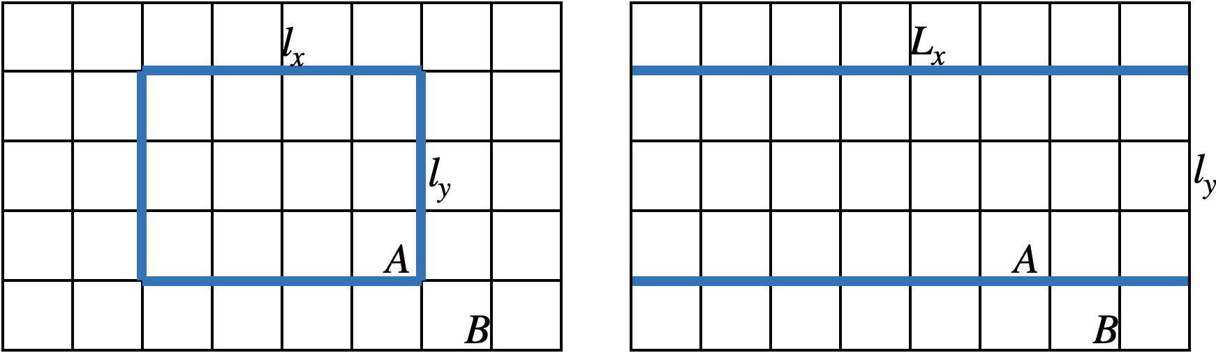
Figure S2: Figure of region $A$ with (left) contractible boundary and (right) $x$-cut.

VI Entanglement entropy : non-contractible boundary

Consider now the region $A$ defined by two non-contractible boundaries running along the $x$-axis and of width $l_{y}$, with the area given by $L_{x}\times l_{y}$. The MES for the $x$-cut (non-contractible boundaries running along the $x$-axis of the torus) is constructed as $\ket{\psi_{\rm MES}}=|G_{\rm MES}|^{-1/2}\sum_{g\in G_{\rm MES}}g\ket{0}$, where the group $G_{\rm MES}$ is spanned by $b_{i}^{x}$, $b_{i}^{y}$, and three WW operators $W_{1}$, $W_{3}$, $W_{5}$. The state thus constructed is an eigenstate of $W_{1},W_{3},W_{5}$ and and the logical operators which are running along the $x$-axis and in $Z$- operator basis. Therefore, the state qualifies as MES Zhang et al. (2012).

Given that the degeneracy factors of $W_{1}$, $W_{3}$, and $W_{5}$ are $N\gcd(L_{x},L_{y},N)/\gcd(L_{x},N)$, $N$, and $\gcd(L_{x},N)$, respectively, the cardinality of $G$ can be expressed as $N^{2L_{x}L_{y}}$. The reason the degeneracy factor of the WW operator is not $N$ is that only the WW operators with specific exponents are considered logical operators. Without loss of generality, we assume that the dependent stabilizers are situated in region $B$. Furthermore, there are two regions near the boundaries where neither $b_{i}^{x}$ nor $b_{i}^{y}$ belongs to both $G_{A}$ and $G_{B}$. We assume that the WW operators are positioned in one of these regions located above region $A$, and we denote this region as region $AB$. This arrangement ensures that there are no dependent stabilizers between the WW operators and the boundary of region $A$.

In this case, the TEE is determined by determined by two types of operations: (i) the operation in $G_{B}$, which can be expressed as the product of $b_{i}^{x}$, $b_{i}^{y}\notin G_{B}$ (ii) the operations in $G_{A}$, which can be expressed as the product of $b_{i}^{x}$, $b_{i}^{y}\notin G_{A}$, and the WW operators $W_{1}$, $W_{3}$, $W_{5}$ loacted in region $AB$. First of all, the operations that satisfy the former conditions are

$$\prod_{b_{i}^{x}\notin G_{B}}b^{x}_{i} \prod_{b_{i}^{y}\notin G_{B}}b^{y}_{i} \left(\prod_{b_{i}^{x},b_{i}^{y}\notin G_{B}}(b^{x}_{i})^{-i_{y}}(b^{y}_{i})^{i_{x}}\right)^{c_{x}}.$$ (S31)

The first two expressions are identical to those of (S24). The third expression is that of (S24) raised to $c_{x}=N/{\rm gcd}(L_{x},N)$ to take account of the periodic boundary conditions for $b_{i}^{y}$. To be faithful to the periodic boundary condition one must be able to impose $(X_{0})^{L_{x}}\equiv 1$ but this is not always the case. On the other hand, $(X_{0})^{c_{x}L_{x}}\equiv 1$ is always true and the number of additional elements in $G_{B}$ is $N^{2}\gcd(L_{x},N)$ instead of $N^{3}$. Therefore, the cardinality of $|G^{x}_{B}|=|G|N^{2}\gcd(L_{x},N)/N^{L_{x}(l_{y}+2)+L_{x}(l_{y}+1)}$.

We have identified four operations that fulfill the latter conditions, with three of them being expressed as:

$$W_{1}\prod_{b_{i}^{x}\in G_{AB}}b_{i}^{x} W_{3}\prod_{b_{i}^{y}\in G_{AB}}b_{i}^{y} W_{5}\prod_{b_{i}^{x}\in G_{AB}}(b_{i}^{x})^{-i_{y}}.$$ (S32)

Here, $G_{AB}$ consists of elements of $G$ that have support exclusively within region $AB$. The stabilizers cancel out the $X$’s of WW operators acting on the region $B$, leaving the remaining operators located on region $A$. The degeneracy factor of three operations in (S32) is same with the degeneracy factors of $W_{1}$, $W_{3}$, and $W_{5}$. The last operation which satisfy the latter condition is well defined when $W_{1}$ with particular exponent $k$ is not a logical operator. This implies that $W_{1}^{k}$ can be represented as the product of $b_{i}^{x}$ and $b_{i}^{y}$. In that case, we can still find $W_{1}^{k}$ located in the region $AB$ within the group $G$. However, $W_{1}^{k}\prod_{b_{i}^{x}\in G_{AB}}b_{i}^{x}$ does not satisfy the latter conditions since $W_{1}^{k}$ includes the product of $b_{i}^{x},b_{i}^{y}\in G_{A}$. Here, we need to focus on the fact that when we express $W_{1}^{A}$ as the product of $b_{i}^{x},b_{i}^{y}\in G_{A}$ included by $W_{1}$, the following expression:

$$W_{1}^{k}(W_{1}^{A})^{{\dagger}}\prod_{b_{i}^{x}\in G_{AB}}b_{i}^{x}$$ (S33)

definitely satisfies the latter condition. We cannot find another operation when $W_{3}$ or $W_{5}$ is not a logical operator. This is because $W_{3}$ is always a logical operator regardless of the lattice size, and when $W_{5}$ is not a logical operator, it is effectively the same as $W_{3}$. Therefore, the degeneracy factors related to $W_{1}$, $W_{3}$, and $W_{5}$ are $N$, $N$, and $\gcd(L_{x},N)$, respectively, and the cardinality of $G_{A}^{x}$ is $N^{L_{x}(2L_{y}-1)}N^{2}\gcd(L_{x},N)$. The results can be summarized:

$$|G| =N^{2L_{x}L_{y}}$$

$$|G_{A}^{x}| =N^{L_{x}(2l_{y}-1)}N^{2}\gcd(L_{x},N)$$

$$|G_{B}^{x}| =|G|N^{2}\gcd(L_{x},N)/N^{L_{x}(l_{y}+2)+L_{x}(l_{y}+1)}$$

$$S_{A}^{x} =4L_{x}\log N-\log(N^{4}\gcd(L_{x},N)^{2}).$$ (S34)

Through a similar calculation, the entanglement entropy $S_{A}^{y}$ for the non-contractible boundary along the $y$-direction is given by $S_{A}^{y}=4L_{y}\log N-\log(N^{4}\gcd(L_{y},N)^{2})$.

We consider the MES characterized by eigenvalues of +1 for all logical operators aligned with the $x$ ($y$)-axis in the case of the $x$ ($y$)-cut, from which we derive the TEE result. It can be shown that the MES with different eigenvalues for corresponding logical operators have the same TEE. This is because the general MES can be described by $U\ket{\psi_{\rm MES}}$, where $U$ is the product of logical operators along the $y$ ($x$)-axis in the case of $x$ ($y$)-cut. Given that $U=U_{A}\otimes U_{B}$ and $\ket{\psi_{\rm MES}}=|G|^{-1/2}\sum_{g\in G}g_{A}\ket{0}_{A}\otimes g_{B}\ket{0}_{B}$, the reduced density matrix of region $A$ for a general MES, denoted as $\rho_{A}$, is expressed as follows:

$$\rho_{A} ={\rm Tr}_{B}[U\ket{\psi_{\rm MES}}\bra{\psi_{\rm MES}}U^{\dagger}]$$

$$={\rm Tr}_{B}[\sum_{g,g^{\prime}\in G}U_{A}g_{A}\ket{0}_{A}\bra{0}_{A}(g_{A}g_{A}^{\prime})^{\dagger}U_{A}^{\dagger}\otimes U_{B}g_{B}\ket{0}_{B}\bra{0}_{B}(g_{B}g_{B}^{\prime})^{\dagger}U_{B}^{\dagger}]$$

$$=\sum_{g\in G,g^{\prime}\in G_{A}}U_{A}g_{A}\ket{0}_{A}\bra{0}_{A}(g_{A}g_{A}^{\prime})^{\dagger}U_{A}^{\dagger}$$

$$=U_{A}\rho_{A}^{\rm MES}U_{A}^{\dagger},$$ (S35)

where $\rho_{A}^{\rm MES}$ is the reduced density matrix of region $A$ for the original MES state. Hence, ${\rm Tr}_{A}[\rho_{A}^{n}]={\rm Tr}_{A}[(\rho_{A}^{\rm MES})^{n}]$, which implies that the EE outcomes for general MES are consistent with (8) for the $x$-cut and (9) for the $y$-cut.

VII TEE and GSD calculation using symmetry defect theory

In the framework of symmetry defect theory, we explicitly calculate the TEE of R2TC using (16). To count the number of $\bf h$- or $\bf g$-invariant anyons among the $a_{\bf 0}$ anyons in (1), we should consider how they transform when they move around the torus:

$$l_{L_{x}+i_{x},i_{y}} =l_{i_{x},i_{y}}+(l_{1}L_{x}~{}{\rm mod}~{}N)\mathtt{p}^{x}-(l_{5}L_{x}~{}{\rm mod}~{}N)\mathtt{g}$$

$$l_{i_{x},L_{y}+i_{y}} =l_{i_{x},i_{y}}+(l_{1}L_{y}~{}{\rm mod}~{}N)\mathtt{p}^{y}+(l_{4}L_{y}~{}{\rm mod}~{}N)\mathtt{g}.$$ (S36)

Clearly, anyons in $C_{\bf 0}^{\bf h}$ must satisfy $l_{1}L_{x}~{}{\rm mod}~{}N=0=l_{5}L_{x}~{}{\rm mod}~{}N$, that is, $l_{1}$ and $l_{5}$ must be multiples of $N/\gcd(L_{x},N)$. Since the other four integers are $\mathbb{Z}_{N}$ without restriction, we find $|C_{\bf 0}^{\bf h}|=N^{4}\gcd(L_{x},N)^{2}$, in agreement with $\gamma_{\rm MES}^{x}$ in (8). A similar reasoning correctly captures $\gamma_{\rm MES}^{y}$.

We calculate the GSD of R2TC using (18) in two steps: first identify distinct defects in $C_{\bf g}$, then further identify those that are invariant under the symmetry defect $\bf h$. Since any one of the defect in $C_{\bf g}$ can be obtained from any other by fusing it with some anyon, and we can find at least one defect $a_{\bf g}\in C_{\bf g}$ which is $\bf h$-invariant, we can express general defects in $C_{\bf g}$ as $a_{\bf g}\otimes l_{i_{x},i_{y}}$. Not all of these defects are necessarily distinct; we need to find a minimal set of anyons that, when fused with $a_{\bf g}$, generates all distinct defects in $C_{\bf g}$. To this end, we employ the known property that all defects in $C_{\bf g}$ are automatically $\bf g$-invariant Barkeshli et al. (2019). The statement of $\bf g$-invariance becomes

$$a_{\bf g}\otimes l_{i_{x},i_{y}}=\,^{\bf g}\left(a_{\bf g}\otimes l_{i_{x},i_{y}}\right)=a_{\bf g}\otimes\,^{\bf g}\left(l_{i_{x},i_{y}}\right)=a_{\bf g}\otimes l_{i_{x},L_{y}+i_{y}}.$$ (S37)

Using (S36), we can equivalently state (S37) as

$$a_{\bf g}\otimes(l_{1}L_{y}~{}{\rm mod}~{}N)\mathtt{p}^{y}\otimes(l_{4}L_{y}~{}{\rm mod}~{}N)\mathtt{g}=a_{\bf g}.$$ (S38)

The coefficients before $\mathtt{p}^{y}$ and $\mathtt{g}$ mean the number of such anyons that, when fused with $a_{\bf g}$, becomes the $a_{\bf g}$ itself. For instance, $L_{y}~{}{\rm mod}~{}N$, $2L_{y}~{}{\rm mod}~{}N$, etc. number of $\mathtt{p}^{y}$ or $\mathtt{g}$ anyons have such a property. By Bezout’s identity, this number is lower-bounded by ${\rm gcd}(L_{y},N)$ for both $\mathtt{p}^{y}$ and $\mathtt{g}$. Then, by limiting the number of $\mathtt{p}^{y},\mathtt{g}$ anyons to be less than ${\rm gcd}(L_{y},N)$, we obtain the desired expression of quasiparticles in $C_{\bf g}$, denoted as $l^{\bf g}_{i_{x},i_{y}}$:

$$l_{i_{x},i_{y}}^{\bf g} =l_{1}\mathtt{e}+((l_{1}i_{x}+l_{2})~{}\text{mod}~{}N)\mathtt{p}^{x}+((l_{1}i_{y}+l_{3})~{}\text{mod}~{}\text{gcd}(L_{y},N))\mathtt{p}^{y}$$

$$+l_{4}\mathtt{m}^{x}+l_{5}\mathtt{m}^{y}+((l_{4}i_{y}+l_{5}i_{x}+l_{6})~{}\text{mod}~{}\text{gcd}(L_{y},N))\mathtt{g},$$ (S39)

where the coefficients before $\mathtt{p}^{y}$ and $\mathtt{g}$ are both mod ${\rm gcd}(L_{y},N)$ rather than mod $N$, as was in (1). The number of distinct $l^{\bf g}$-anyons is equal to $|C_{\bf g}|$ and is $N^{4}\gcd(L_{y},N)^{2}$.

The subset of $C_{\bf g}$ that are $\bf h$-invariant satisfies $l_{i_{x},i_{y}}^{g}=l_{L_{x}+i_{x},i_{y}}^{g}$ since $a_{\bf g}$ was assumed to be $\bf h$-invariant. Then, we can get

$$l_{1}L_{x}~{}{\rm mod}~{}N=0=l_{5}L_{x}~{}{\rm mod}~{}\gcd(L_{y},N).$$ (S40)

This implies that $l_{1}$ and $l_{5}$ must be multiples of $N/\gcd(L_{x},N)$ and $\gcd(L_{y},N)/\gcd(L_{x},L_{y},N)$, respectively. Counting the distinct set of integers $l_{1}-l_{6}$ in (S39) consistent with (S40), we find $|C_{\bf g}^{\bf h}|={\rm GSD}$. Similar consideration applies to $|C_{\bf h}^{\bf g}|$ with the same result.

VIII Spurious entanglement entropy

We analyze the spurious entanglement of the non-topological model proposed in Williamson et al. (2019), using our idea of taking the bulk product of stabilizers to arrive at the boundary product. We conclude the boundary product in this case does not fully encircle the region $A$, and also find some dependence on the shape of the boundary.

The model Williamson et al. (2019) is defined on a square lattice, comprising two stabilizers:

$$IZ-IZ~{}~{}~{}~{}~{}~{}~{}~{}~{}~{}~{}~{}~{}~{}~{}ZX-ZI$$

$$a=~{} ~{}|~{}~{}~{}~{}~{}~{}~{}|~{}~{}~{}~{}~{}~{}~{}~{}~{}~{}~{}b=~{}~{}|~{}~{}~{}~{}~{}~{}~{}|$$

$$IZ-XZ~{}~{}~{}~{}~{}~{}~{}~{}~{}~{}~{}~{}~{}~{}~{}ZI-ZI.$$ (S41)

Two $\mathbb{Z}_{2}$ degrees of freedom are assigned to each vertex corresponding to the first and the second Pauli operator in the above. The (unique) ground state of this model is

$$\ket{\psi}=|G|^{-1/2}\sum_{g\in G}g\ket{0+},$$ (S42)

where the group $G$ is generated by $a$’s and $\ket{0+}$ satisfies $IX\ket{0+}=ZI\ket{0+}=\ket{0+}$ for arbitrary vertices.

We evaluate the entanglement entropy of $|\psi\rangle$ first for a $l_{x}\times l_{y}$ square region $A$ as depicted in Fig. S2. The operations that significantly influence the TEE are the elements of $G_{B}$, which are the product of $a\notin G_{B}$, and the elements of $G_{A}$, which are the product of $a\notin G_{A}$. We can identify the operation satisfying the former condition, depicted in Fig. S3 (a). The operation is the multiplication of $a$’s and encircled by the yellow loop. This operation in terms of $X$ and $Z$ takes the form of a square bracket encompassing a part of the boundary, signifying that the count of such operations is expected to vary based on the shape of the region. The entanglement entropy result is summarized as

$$|G| =2^{L_{x}L_{y}}$$

$$|G_{A}| =2^{l_{x}l_{y}}$$

$$|G_{B}| =|G|2^{-(l_{x}+2)(l_{y}+2)+1}$$

$$S_{A} =(2l_{x}+2l_{y})\log 2-\log 2,$$ (S43)

and TEE is equal to $\log 2$. We can easily check that the TEE depends on the shape of the boundary. By altering the boundary, as depicted in Fig. S3 (b), we can identify two operations influential to the TEE, each one encircled by yellow loop.

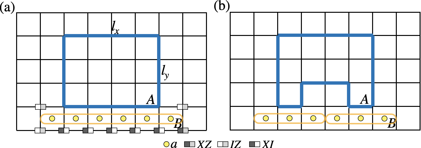
Figure S3: (a)An operation satisfying the condition of being an element of $G_{B}$ and the product of $a\notin G_{A}$. The operation is influential to the TEE and represented by by the encirculed yellow loop. (b) Two operations, represented by yellow loops and influential to the TEE, are depicted.

This observation deviates from the well-known concept of TEE and should be regarded as spurious TEE. Conversely, if the operation takes the form of a WW loop encircling the entire boundary of the region, the number of elements cannot depend on the shape of the region, indicating a genuine TEE. Based on the analysis conducted in this simple example, we can confidently assert that there are no instances of spurious TEE in the entanglement entropy calculation for R2TC. The identified operations are the the form of WW loop, thereby eliminating any possibility of spurious TEE contributions.

IX Tensor Network calculation: entanglement entropy for R2TC

In this section, we demonstrate how to express the MES of R2TC using a Tensor Network (TN) framework, building upon the TN wavefunction introduced in Ref. Oh et al., 2023. By examining the local gauge symmetry of tensors as summarized in Ref. Oh et al., 2023, when both system sizes $L_{x}$ and $L_{y}$ are multiples of $N$, the TN wavefunction serves as a ground state of R2TC and is simultaneously an eigenstate of $W_{1}$, $W_{2}$, $W_{3}$, $W_{4}$, $\widetilde{W}_{5}$, and $\widetilde{W}_{6}$, all with eigenvalues equal to 1. However, when we consider a $y$-cut, the MES should be an eigenstate for the WW operators $\widetilde{W}_{1}$, $W_{2}$, $\widetilde{W}_{3}$, $W_{4}$, $\widetilde{W}_{5}$, and $W_{6}$ simultaneously. Therefore, the TN wavefunction originally proposed in Ref. Oh et al., 2023 is not an MES and requires some modifications to transform it into an MES.

The process of modifying the TN wave function to become a MES for $y$-cut can be broken down into three distinct steps. The first step is to enforce TN wavefunction to be an eigenstate of $\widetilde{W}_{1}$ instead of $W_{1}$. In the second step, we make further modifications to the TN to ensure wavefunction to be an eigenstate of $\widetilde{W}_{3}$ instead of $W_{3}$. Finally, in the third step, we enforce the wavefunction to be eigenstate of $W_{6}$ instead of $\widetilde{W}_{6}$.

IX.1 Review: Tensor network wavefunction

In this subsection, we review the TN wavefunction introduced in Ref. Oh et al., 2023, which is suggested as one of the TN formulas responsible for one of the R2TC ground states. The TN wavefunction is composed of three local tensors $T_{udlr}$, $g_{udlr}^{s_{1}s_{2}}$, and $g_{udlr}^{s_{0}}$ and can be represented as below:

$$\includegraphics[width=260.17464pt]{./01-tn-fig-eq/eq-TN-r2tc.png}.$$ (S44)

The indices $s_{1},s_{2},s_{0}$ represent physical indices corresponding to the local ${\mathbb{Z}}_{N}$ orbitals of R2TC, while the indices $u,d,l,r$ are virtual indices with ${\mathbb{Z}}_{N}$ character that are contracted out in the finial expression. The first two tensors are defined as

$$T_{udlr}= \delta_{u+r-(l+d),0}, g_{udlr}^{s_{1}s_{2}}=\left(\delta_{l,r}\delta_{l,s_{1}}\right)\left(\delta_{d,u}\delta_{d,s_{2}}\right).$$ (S45)

Note that the delta is implemented by mod $N$ throughout this section. To define the third local tensor, we need to introduce following isometry tensor:

$$P_{s_{1}s_{1}}^{s_{0}}=\delta_{s_{0},s_{1}+s_{2}}.$$ (S46)

Then the third local tensor is defined as

$$g_{udlr}^{s_{0}}=P_{s_{1}s_{1}}^{s_{0}}g_{udlr}^{s_{1}s_{2}}.$$ (S47)

Here, the summation for repeated indices is implied.

IX.2 Loop-gas interpretation

As mentioned in above, the TN wavefunction is an eigenstate of WW operators without tilde; $W_{1}$, $W_{2}$, $W_{3}$, and $W_{4}$. To gain an intuitive understanding of this, we introduce the concept of a loop-gas configuration picture. From this point onward, we confine our analysis to the $\mathbb{Z}_{2}$ case for the sake of clarity and simplicity in the subsequent discussion. The concepts and principles discussed can be readily extended to the general $\mathbb{Z}_{N}$ case without any difficulty. Furthermore, our discussion will primarily center on scenarios where both system sizes, $L_{x}$ and $L_{y}$, are even. To say it in advance, we have numerically confirmed that the TN achieved by the discussion below also serves as a MES for system size under various conditions.

In $\mathbb{Z}_{2}$ case, one can understand the virtual legs as being occupied by a loop when the corresponding virtual index has a value of $1$, and being unoccupied when the the value is $0$. Using this interpretation, we can translate the TN wavefunction in Eq. (S44) into the loop-gas configuration picture. In doing so, we discover that the TN wavefunction is essentially an equal superposition of every possible closed-loop configurations, both on the solid and dotted lattices, respectively. An example of the closed-loop configuration is given in Fig. S4 (a).

This is attributed to the role played by $T_{udlr}$, which acts to ensure the closure of all loops. It is because, from the definition of $T_{udlr}$ in Eq. (S45), whenever a loop enters to $T_{udlr}$, it must also exit. It is important to note that the closed-loop condition enforced by $T_{udlr}$ facilitates the presence of non-contractible loop configurations around the torus system.

Now, we consider how the WW operator $W_{1}$ acts on the TN wavefunction. To see that, we need to understand the action of a local Pauli-$X$ operator on the $g$ tensors. Referring to the definition in Eq. (S45), one can observe that when $s_{1}=1$ ($s_{2}=1$), a solid (dotted) line crossing the $g_{udlr}^{s_{1}s_{2}}$ tensor is occupied by a horizontal (vertical) loop, while it remains empty when $s_{1}=0$ ($s_{2}=0$). Additionally, for either the dotted or solid lines crossing the $g_{udlr}^{s_{0}}$, they are occupied by horizontal or vertical lines when $s_{0}=1$, and both lines are either empty or occupied by both horizontal and vertical lines when $s_{0}=0$. Consequently, applying a local Pauli-$X$ operator to the $g$ tensors leads to a switch in the occupation state as described.

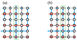
Figure S4: Illustrations of R2TC loop configurations. Blue lines denote loops on the dotted lattice, while orange lines represent loops on the solid lattice. The physical indices are omitted. The position where $W_{6}$ is applied is marked by closed green dashed-loop. (a) A configuration comprising exclusively of closed loops. (b) A configuration featuring a single isolated vertical loop. All other loops, apart from the vertical one at rightmost dotted column, are closed.

The WW operator $W_{1}$ acts by applying Pauli-$X$ operators to lattice sites positioned on the non-contractible dotted line defined along the $x$-axis. Building upon the insights from the previous paragraph, it becomes clear that the action of $W_{1}$ involves the insertion of a horizontal non-contractible loop in the dotted lattice. It is worth noting that in the context of our $\mathbb{Z}_{2}$ system, the insertion of a non-contractible loop is equivalent to toggling the number of non-contractible loops between even and odd. Since the TN wave function described in Eq. (S44) already includes all possible closed loop configurations, encompassing both cases containing an even or odd number of non-contractible loops, the operations performed by the $W_{1}$ operator do not alter the TN wave function. This property results in the TN wavefunction being an eigenstate of $W_{1}$ with an eigenvalue of $1$. By applying a similar rationale as discussed above, one can ascertain that the remaining WW operators, $W_{2}$, $W_{3}$, and $W_{4}$ also function by inserting horizontal or vertical non-contractible loops into the dotted or solid lattices, respectively. Employing analogous logic, it can be deduced that the TN wavefunction defined in Eq. (S44) is likewise an eigenstate of $W_{2}$, $W_{3}$, and $W_{4}$ with an eigenvalue of $1$.

Now we will delve into the three steps involved in transforming the TN wavefunction into an MES within the framework of loop-gas configurations, addressing each step individually. The first step is to enforce it to be an eigenstate of $\widetilde{W}_{1}$ instead of $W_{1}$. These operators are in anti-commutation relation: $W_{1}\widetilde{W}_{1}=-\widetilde{W}_{1}W_{1}$. We shall now represent the eigenstates of $\widetilde{W}_{1}$ with the eigenvalues $1$ and $-1$, as $|0\rangle$ and $|1\rangle$, respectively. We use the representations $0$ and $1$ to emphasize that the tilde WW operator $\widetilde{W}_{1}$ is composed of the product of Pauli-$Z$ operators. The action of $W_{1}$ interchanges these two states, transforming $|0\rangle$ into $|1\rangle$ and vice versa. The eigenstates of $W_{1}$ can be expressed as an equal superposition of these two states, taking the form of $1/\sqrt{2}(|0\rangle\pm|1\rangle\bigr{)}$ with eigenvalue $\pm 1$. The TN wavefunction is an eigenstate of $W_{1}$ with eigenvalue $1$, and hence taking form $1/\sqrt{2}(|0\rangle+|1\rangle\bigr{)}$. Furthermore, combining with the discussion of the closed-loop configuration above, it can be inferred that either $|0\rangle$ or $|1\rangle$ correspond to an equal superposition of every closed loop configuration, with the distinction being that they contain either an even or odd number of horizontal non-contractible loops in the dotted lattice.

Enforcing the TN wavefunction to be an eigenstate of $\widetilde{W}_{1}$ can be understood as transforming the original wavefunction from the form $(|0\rangle+|1\rangle\bigr{)}$ into either $|1\rangle$ or $|0\rangle$. In the loop-gas configuration picture, this translates to ensuring that the TN wavefunction contains either an even or odd number of horizontal non-contractible loops in the dotted lattice. This marks the first step in the process of making the TN wavefunction an MES.

Expanding on this idea, one can observe that enforcing the TN wavefunction to be an eigenstate of $\widetilde{W}_{3}$ is equivalent to guaranteeing that the TN wavefunction comprises only even or odd numbers of horizontal non-contractible loops in the solid lattice. This step is evidently the second stage in the modifying the TN wavefunction into an MES.

The final step involves ensuring that the TN becomes an eigenstate of $W_{6}$ instead of being an eigenstate of $\widetilde{W}_{6}$. The original TN wave function given in Eq. (S44) consists solely of closed-loop configurations as in Fig. S4(a). However, when we apply $W_{6}$, it introduces a vertical dashed line on the dotted lattice, as illustrated in Fig. S4(b).

Let’s consider the anti-commutation relation $W_{6}\widetilde{W}_{6}=-W_{6}\widetilde{W}_{6}$. The eigenstates of $\widetilde{W}_{6}$ are denoted as $|0\rangle$ and $|1\rangle$, corresponding to eigenvalues $1$ and $-1$, respectively. The action of $W_{6}$ interchanges these two states, transforming $|0\rangle$ into $|1\rangle$ and vice versa. Consequently, it can be deduced that the original TN wavefunction takes the form of $|0\rangle$, whereas the TN wavefunction containing a single vertical dashed line on the dotted lattice, denoted as $W_{6}|0\rangle$, takes the form of $|1\rangle$.

Since the MES is required to be an eigenstate of $W_{6}$, we must ensure that it takes the form of $|0\rangle\pm|1\rangle$. This is equivalent to constructing the TN as a superposition of two sets of loop configurations. One set consists solely of closed-loop configurations (Fig. S4(a)), while the other includes a single vertical dashed loop on the dotted lattice (Fig. S4(b)). This completes the final step of transforming the original TN wavefunction into an MES.

IX.3 Tensor network implementation

In the following, we will provide a detailed explanation of how to implement these three steps within the framework of TN one by one. In first step, we need to ensure that the TN wavefunction only contains even-number of horizontal non-contractible closed loop on dotted lattice. This can be simply done by pick any single vertical line form dotted lattice. Then attaching a new tensor $\Omega_{udlr}$ to $T_{udlr}$ tensors located on the vertical line as

(S48)

Here, the tensor $\Omega_{udlr}$ is defined by

$$\Omega_{udlr}=\delta_{l,r}\delta_{l,u-d}.$$ (S49)

To grasp how the tensor $\Omega_{udlr}$ constrains the quantity of horizontal non-contractible closed loops, let’s focus on a vertical dotted bond connected to $\Omega_{udlr}$. Let’s assume we initiate with a value of $0$ for the virtual bond and traverse along the $y$-direction. Whenever we encounter a horizontal loop that crosses through $\Omega_{udlr}$, the value of the vertical bond toggles between $0$ and $1$, and vice versa. If a configuration contains an odd number of non-contractible horizontal loops on the dotted lattice, we will encounter the horizontal loop an odd number of times during the round trip, causing the virtual bond to end up with a value of $1$. Since the initial value of the virtual bond was $0$, this scenario leads to a mismatch and is therefore excluded from the tensor contraction. Consequently, we obtain configurations that exclusively consist of an even number of horizontal non-contractible loops on the dotted lattice.

Similarly, by additionally attaching $\Omega_{udlr}$ to $T_{udlr}$ tensors located at any single vertical line form solid lattice as

(S50)

Note that in the remaining vertical lattice lines, $\Omega_{udlr}$ is not connected. As a result, the TN wave function now exclusively comprises loop configurations with an even number of horizontal non-contractible loops on each lattice. This condition ensures that the TN wave function becomes an eigenstate of both $\widetilde{W}_{1}$ and $\widetilde{W}_{3}$ marking the successful completion of the first and second steps.

The implementation of third step, the final step of enforcing the TN wavefunction being an MES, encompass not only just attaching additional auxiliary tensor, involves more than just the attachment of an additional auxiliary tensor. It also necessitates the modification of certain local tensors $T{udlr}$. Similar to the first and second step, we pick a single vertical lines from dotted lattice, and replace the tensors $T_{udlr}$ with $T_{udlr;m}$, which can be graphically illustrated as

$$\includegraphics[width=195.12767pt]{./01-tn-fig-eq/eq-TN-modified-T.pdf}.$$ (S51)

Here, the first image provides a top view, while the second offers a side view from a slanted perspective. The leg representing $\mathbb{Z}_{2}$ index $m$ goes the direction penetrating the surface, in contrary to the physical indices in Eq. (S44) comes in the direction emerging from the surface. Its mathematical definition is given by

$$T_{udlr;m}= \delta_{u+r-(l+d),m},$$ (S52)

Now, $T_{udlr;m}$ allows termination of a loop at the point when $m=1$. Note that $T_{udlr;0}=T_{udlr}$.

Afterward, we attach the $\Theta^{m}_{ud}$ right below the $T_{udlr;m}$ as

$$\includegraphics[width=216.81pt]{./01-tn-fig-eq/eq-TN-modified-T-2.pdf}.$$ (S53)

Here, $\Theta^{m}_{u^{\prime}d^{\prime}}$ is defined by

$$\Theta^{m}_{u^{\prime}d^{\prime}}=\delta_{m,u^{\prime}}\delta_{u,d^{\prime}}$$ (S54)

Consequently, the ultimate structure of the TN wave function takes the form:

$$\includegraphics[width=195.12767pt]{./01-tn-fig-eq/eq-TN-r2tc-w1-w3-w6.pdf}.$$ (S55)

With the introduction of $\Theta^{m}_{u^{\prime}d^{\prime}}$, we introduce an additional vertical line on the “lower level” of the original lattice, linking the indices $u^{\prime}$ and $d^{\prime}$. As defined in Eq. (S54), this vertical line allows only two configurations: either a closed non-contractible loop occupies the line, or the line remains empty. The configurations of the empty line correspond to the configurations prior to the third step. In the case of an occupied line, the configurations encompass a single vertical dashed loop on the dotted lattice, as depicted in Fig. S4(b). This completes the entire step of transforming the TN wavefunction into a MES.

Numerically, we have confirmed that the wavefunction constructed by the TN given in Eq. (S55) is MES for any cases of system size. Specifically, we have calculated the expectation values for WW operator in Table 1 being $1$ for the TN wavefunction.