Qubit Count Reduction by Orbital Optimization for Variational Quantum Excited States Solvers

Abstract

We propose a state-averaged orbital optimization scheme for improving the accuracy of excited states of the electronic structure Hamiltonian for use on near-term quantum computers. Through extensive benchmarking of the method on various small molecular systems, we find that the method is capable of producing more accurate results than fixed basis FCI while simultaneously using fewer qubits. In particular, we show that for H2, the method is capable of matching the accuracy of FCI in the cc-pVTZ basis (56 qubits) while only using 14 qubits.

Duke]Department of Physics, Duke University Fudan]School of Mathematical Sciences, Fudan University Duke]Department of Mathematics, Duke University Department of Physics, Duke University Department of Chemistry, Duke University

1 Introduction

One of the early applications for quantum computers is expected to be the electronic structure problem ¹, however, the error stemming from the basis set truncation in the second quantization formulation will likely present a major obstacle for realizing accurate solutions for academically and industrially relevant chemical systems ^{2, 3, 4}. If no resource reduction techniques are employed, one qubit is needed for each spin-orbital. As a result of the limited number of qubits on current hardware, experimental demonstrations have been limited to small molecules represented by small basis sets ^{5, 6, 7, 8}. Several methods have been developed for more compact basis set representations in both the classical and quantum settings. Explicitly correlated methods ^{9, 10, 11, 12} apply a similiarity transformation to the problem Hamiltonian that has an explicit dependence on the coordinates of the electrons. The intuition behind this is that such basis sets may be able to efficiently capture effects from electron-electron interactions which are often the cause of the inefficiency of fixed single-particle basis set representations ^{13, 14}. Downfolded effective Hamiltonian techniques ^{15, 16, 17, 18, 19} take a full orbital space Hamiltonian, unitarily transform it according to an excitation operator that includes excitations outside of a given active space, then project it onto the active space. Through this process, an effective Hamiltonian is produced which includes correlation effects from outside the active space, but which is low-dimensional and acts only on the active space. Orbital optimization methods ^{20, 21, 22, 23, 24, 25, 26} introduce the elements of a similarity transformation to be optimized in conjunction with the parameters of an eigensolver minimization problem. These two minimization problems are typically solved in an alternating fashion until some stopping criteria are reached. Orbital optimization schemes such as quantum CASSCF ²⁵ operate by first choosing an active space from a full orbital space, then unitarily transforming the orbitals according to a coupled-cluster style ansatz. In this work we extend OptOrbVQE ²⁰, which finds the ground state in an optimized basis, to the problem of finding excited states of electronic structure Hamiltonians. The main differences between OptOrbVQE and other orbital optimization ground state solvers are that 1. the orbital rotation does not take the form of a parameterized ansatz and 2. the selection of an active space is not required. Instead, the orbital transformation takes the form of a partial unitary matrix. Thus no chemical intuition or selection of orbitals based on energy is required to choose an active space and we can optimize over a more general set of rotations.

2 Excited States Quantum Eigensolvers

Hybrid quantum-classical variational methods for finding eigenvalues of chemical Hamiltonians operate by classically minimizing an objective function constructed from quantities measured on a quantum computer. For example, to find the ground state of a Hamiltonian $\hat{H}$ we would first prepare a parametrized state $\ket{\psi(\boldsymbol{\theta})}$ on the quantum computer, measure the expectation value of $\hat{H}$, and carry out the minimization problem:

$$\min_{\boldsymbol{\theta}}\bra{\psi(\boldsymbol{\theta})}\hat{H}\ket{\psi(\boldsymbol{\theta})}$$ (1)

classically. This is the original formulation of the variational quantum eigensolver ^{27, 28} (VQE). In order to extend this method to low-lying excited states, the mutual orthogonality of these states must be accounted for. Several methods have been proposed that accomplish this. SSVQE ²⁹ and MCVQE ³⁰ are state-averaged approaches which apply a parameterized circuit $\hat{U}(\boldsymbol{\theta})$ to a set of mutually orthogonal initial states $\{\ket{\psi_{i}}\}$, then minimize an objective function of the form:

$$f(\boldsymbol{\theta})=\sum_{i}w_{i}\bra{\psi_{i}}\hat{U}^{\dagger}(\boldsymbol{\theta})\hat{H}\hat{U}(\boldsymbol{\theta})\ket{\psi_{i}}$$ (2)

where $\{w_{i}\}$ is a set of positive, real-valued weights. The main difference between MCVQE and SSVQE is that MCVQE chooses the weights $\{w_{i}\}$ to be equal, whereas SSVQE chooses them to not be equal. At first glance this difference seems trivial, however it should be noted that unequal weights corresponds to a global minimum comprised of the low-lying eigenvectors, whereas an equal weighting corresponds to a global minimum comprised of states which span the low-lying eigenspace. MCVQE adds a classical post-processing step which diagonalizes these states in this low-dimensional eigenspace to acquire the low-lying eigenvectors. It is unclear which of these approaches is advantageous or if their convergence is equivalent in practice. Other excited states methods such as qOMM ³¹ and VQD ³² take overlap-based approaches to enforcing the mutual orthogonality of the solution by including penalty terms in the objective function which vanish when pairs of states are orthogonal. Thus, the orthogonality is enforced only at the global minimum rather than at every point in the cost function landscape.

3 State-Averaged Orbital Optimization

In OptOrbVQE we take the electronic structure Hamiltonian in its fermionic second-quantization representation:

$$\hat{H}=\sum_{p,q=1}^{M}h_{pq}\hat{a}^{\dagger}_{p}\hat{a}_{q}+\frac{1}{2}\sum_{p,q,r,s=1}^{M}v_{pqrs}\hat{a}^{\dagger}_{p}\hat{a}^{\dagger}_{q}\hat{a}_{s}\hat{a}_{r},$$ (3)

and rotate the set of $M$ orbitals $\{\psi_{1},\psi_{2},...,\psi_{M}\}$ according to the partial unitary transformation $\hat{V}$:

$$\tilde{\psi_{i}}=\sum_{j}^{M}\hat{V}_{ji}\psi_{j}$$ (4)

resulting in a new set of $N<M$ orbitals $\{\tilde{\psi}_{1},\tilde{\psi}_{2},\dots,\tilde{\psi}_{N}\}$. This is equivalent to transforming the Hamiltonian as:

$$\begin{split}&\tilde{H}(\hat{V})=\sum_{p^{\prime},q^{\prime}=1}^{N}\sum_{p,q=1}^{M}h_{pq}\hat{V}_{pp^{\prime}}\hat{V}_{qq^{\prime}}\tilde{a}^{\dagger}_{p^{\prime}}\tilde{a}_{q^{\prime}}\\ &+\frac{1}{2}\sum_{p^{\prime},q^{\prime},r^{\prime},s^{\prime}=1}^{N}\sum_{p,q,r,s=1}^{M}v_{pqrs}\hat{V}_{pp^{\prime}}\hat{V}_{qq^{\prime}}\hat{V}_{ss^{\prime}}\hat{V}_{rr^{\prime}}\tilde{a}^{\dagger}_{p^{\prime}}\tilde{a}^{\dagger}_{q^{\prime}}\tilde{a}_{s^{\prime}}\tilde{a}_{r^{\prime}.}\end{split}$$ (5)

The orbital optimization then corresponds to minimizing the expectation value of this Hamiltonian with respect to a fixed quantum state $\hat{U}(\boldsymbol{\theta})\ket{\psi_{ref}}$ provided by a quantum eigensolver. The total minimization problem is then given by:

$$\min_{\begin{subarray}{c}\boldsymbol{\theta}\\ \hat{V}\in\mathcal{U}(M,N)\end{subarray}}\bra{\psi_{\text{ref}}}\hat{U}^{\dagger}(\boldsymbol{\theta})\tilde{H}(\hat{V})\hat{U}(\boldsymbol{\theta})\ket{\psi_{\text{ref}}}$$ (6)

where $\mathcal{U}(M,N)$ is the set of $M\times N$ real partial unitary matrices. The simplest way to generalize this problem is to consider Eq. 2 to be a function of both $\boldsymbol{\theta}$ and $\hat{V}$:

$$f(\boldsymbol{\theta},\hat{V})=\sum_{i}w_{i}\bra{\psi_{\text{ref},i}}\hat{U}^{\dagger}(\boldsymbol{\theta})\tilde{H}(\hat{V})\hat{U}(\boldsymbol{\theta})\ket{\psi_{\text{ref},i}}$$ (7)

and minimize the resulting state-averaged analog problem of Eq. 6:

$$\min_{\begin{subarray}{c}\boldsymbol{\theta}\\ \hat{V}\in\mathcal{U}(M,N)\end{subarray}}f(\boldsymbol{\theta},\hat{V}).$$ (8)

Such state-averaged analogs of other orbital optimization schemes ^{26, 21} have previously been explored in the literature. Thus, we expect a state-averaged analog of OptOrbVQE to also perform well. It is worth noting that an overlap-based orbital optimization objective function has been proposed in the classical literature ³³, which allows for a separate optimal basis to be computed for each excited state. The authors claim that this allows for more accurate excitation energies to be computed. The method assumes the availability of the CI coefficients found by the eigensolver, which would require exponentially-expensive full state tomography to acquire in the quantum computing setting.

The total minimization problem Eq. 8 is divided into two subproblems: minimization with respect to the ansatz parameters $\boldsymbol{\theta}$ and minimization with respect to $\hat{V}$. These two subproblems are solved in an alternating fashion, where one is fixed while the other is varied. The optimal parameters for one subproblem are then used for the initialization of the next run of the other until some global stopping criteria are met. For example, for a given optimal $\hat{V}$ we can compute $\tilde{H}(\hat{V})$ and carry out a quantum excited states solver to find an optimal $\boldsymbol{\theta}$ in the rotated basis. For a given $\boldsymbol{\theta}$ found by a quantum excited states solver, we can compute the 1 and 2-RDMs with respect to each state in the set of computed excited states $\{\hat{U}(\boldsymbol{\theta})\ket{\psi_{\text{ref},i}}\}$, then vary Eq. 8 with respect to $\hat{V}$. As was done for OptOrbVQE, we explicitly state the super and subscript notation used for the total problem to avoid confusion:

• The subscript $l$ will index the iteration number in the minimization problem where $\hat{V}$ is varied.

• The subscript $m$ will index the iteration number in the minimization problem where $\boldsymbol{\theta}$ is varied.

• The subscript $n$ will index a global “outer loop” iteration number that characterizes how many times both subproblems have been carried out.

• The superscript opt will denote the optimal parameter found in each subproblem for a given outer loop iteration number.

We now give an explicit step-by-step procedure for the total problem:

1. Set $n=0$. Choose an initial partial unitary $\hat{V}_{n=0,l=0}$, an initial set of ansatz parameters $\boldsymbol{\theta}_{n=0,m=0}$, and a stopping threshold $\epsilon$.

2. Calculate $\tilde{H}(\hat{V})$ on a classical computer and run a quantum eigensolver algorithm to obtain $\boldsymbol{\theta}_{n}^{opt}$.

3. If $\lvert f(\boldsymbol{\theta}_{n}^{opt},\hat{V}_{n-1}^{opt})-f(\boldsymbol{\theta}_{n-1}^{opt},\hat{V}_{n-2}^{opt})\rvert<\epsilon$, halt the algorithm. Else, continue to the next step.

4. Measure the 1 and 2-RDMs with respect to the set of states $\{\hat{U}(\boldsymbol{\theta}_{n}^{opt})\ket{\psi_{\text{ref},i}}\}$ on a quantum computer.

5. Using the 1 and 2-RDMs from the previous step, minimize Eq. 8 with respect to $\hat{V}_{n}$ to obtain $\hat{V}_{n}^{opt}$.

6. Set $n=n+1$, $\hat{V}_{n+1,l=0}=\hat{V}_{n}^{opt}$, and $\boldsymbol{\theta}_{n+1,m=0}=\boldsymbol{\theta}_{n}^{opt}$. Optionally, a small random perturbation can be added to the latter two quantities. Repeat steps 2-6.

Step 5 requires the use of a classical optimizer which constrains $\hat{V}$ to be a partial unitary. Several methods which do this exist ^{34, 35, 36, 37}, but in our work we use an orthogonal projection method ³⁸. In general, $\boldsymbol{\theta}$ and $\hat{V}_{n+1,l=0}$ could be any real vector and real partial unitary, respectively, however it is intuitive to use information from the $n$th outer loop iteration to inform this choice. In our work we choose $\boldsymbol{\theta}_{n+1,l=0}=\boldsymbol{\theta}_{n}^{opt}$ and $\hat{V}_{n+1,l=0}=\mathrm{orth}(\hat{V}_{n}^{opt}+\mathrm{Rand(M,N))}$, where

$$\mathrm{orth}(A)=AQ\Lambda^{-\frac{1}{2}}Q^{\dagger}$$ (9)

and $\mathrm{Rand(M,N)}$ is an $M\times N$ matrix whose elements are sampled from a normal distribution with average 0 and standard deviation 0.01. In Eq. 9, $Q$ is a matrix whose columns are the eigenvectors of $A^{\dagger}A$ and $\Lambda$ is a diagonal matrix whose entries are the eigenvalues of $A^{\dagger}A$. Additionally, although Eq. 8 is written as a state-averaged function of $\boldsymbol{\theta}$, step 2 does not necessarily need to be carried out using a state-average quantum eigensolver. The only requirement is that the solver returns solution states to be used for the calculation of 1 and 2-RDMs. Overlap-based methods such as qOMM ³¹ and VQD ³² could be used, however for our work we test MCVQE ³⁰ and SSVQE ²⁹.

4 Numerical Results

The code used for our numerical simulations is an extension of the functionality provided by the open source package Qiskit ³⁹. Qiskit provides an implementation of VQE ^{27, 28}, which we have modified to produce implementations of SSVQE ²⁹ and MCVQE ³⁰. The code for the state-averaged orbital optimization is a modification of the code used in our ground state orbital optimization work ²⁰, with the main modification being the objective function to be minimized. The Qiskit package versions used are Qiskit-Aer 0.12.0, Qiskit-Nature 0.4.5, and Qiskit-Terra 0.23.2. The 1 and 2-body integrals are obtained through the PySCF ⁴⁰ electronic structure driver in Qiskit, which uses PySCF to perform a restricted Hartree-Fock problem to obtain the un-optimized molecular integrals. Configuration interaction circuits are obtained in two steps. First, the truncated Hamiltonians are constructed from the 1 and 2-body integrals using the Slater-Condon rules ¹, which are then exactly diagonalized using NumPy ⁴¹. The reasons why we do not use PySCF’s configuration interaction implementation are two-fold: (1) PySCF does not have an CIS implementation and (2) We have found that PySCF’s CISD implementation does not always produce orthogonal CI wavefunctions, with fidelity between two states being as large as on the order of $10^{-1}$, even in the case where the corresponding eigenvalues are not degenerate. This is problematic for quantum algorithms such as SSVQE and MCVQE which require that the initial states be mutually orthogonal.

This statevector can then be used to initialize a circuit using Qiskit’s arbitrary statevector initialization implementation. We note that although this particular implementation requires the storage of an exponentially large statevector in classical memory, in principle configuration interaction state preparation on a quantum computer could be done in a completely sparse manner with resources scaling polynomially with the number of qubits. For example, it has been shown that Givens rotations are universal for preparing chemically-motivated states with the Jordan-Wigner mapping ⁴². The authors also give a general procedure for preparing an arbitrary statevector. In Appendix B we give an explicit example of how the particular case of arbitrary CIS statevectors can be prepared on a quantum computer, which may be of independent interest. Whether or not an efficient analogous procedure can be developed for CISD states is not discussed here, however in our simulations we include CISD initializations to investigate whether or not doing so would lead to further improvement. We also utilize an "excited Hartree-Fock" initialization that consists of the Hartree-Fock state and the lowest energy singly-excited states from it. In this paper, we will refer to this initialization as just "Hartree-Fock" or "HF".

In Qiskit, one can use any ansatz circuit as a base pattern to be repeated $n$ times, increasing the circuit depth and number of parameters by a factor of $n$. In our simulations we use Qiskit’s implementation of the UCCSD ansatz ⁴³ as a circuit block pattern to be repeated for various values of $n$. We denote this as $n$-UCCSD. The classical optimizer used for all test instances is L-BFGS-B ⁴⁴. The FCI reference values are calculated using CDFCI. ⁴⁵ All orbital-optimized tests are run using Qiskit’s AerSimulator in noiseless statevector mode.

4.1 H2

We begin with our results for the simplest model tested, H2 at the near-equilibrium bond distance 0.735 Å, which are given in Fig. 1. We use cc-pVQZ (120 spin-orbitals) as the starting basis and reduce the active space for even numbers of spin-orbitals from 4 to 14 using the proposed orbital optimization scheme. The difference between the average orbital optimized energy and that of FCI (over the ground and excited states) in the cc-pVTZ basis is plotted as a function of the outer loop iteration. Tests using both 2 and 3-UCCSD are included to investigate the effect of increasing the ansatz expressiveness in the algorithm. Both eigensolvers are initialized with configuration interaction singles (CIS) states. SSVQE is additionally tested using the Hartree-Fock initialization.

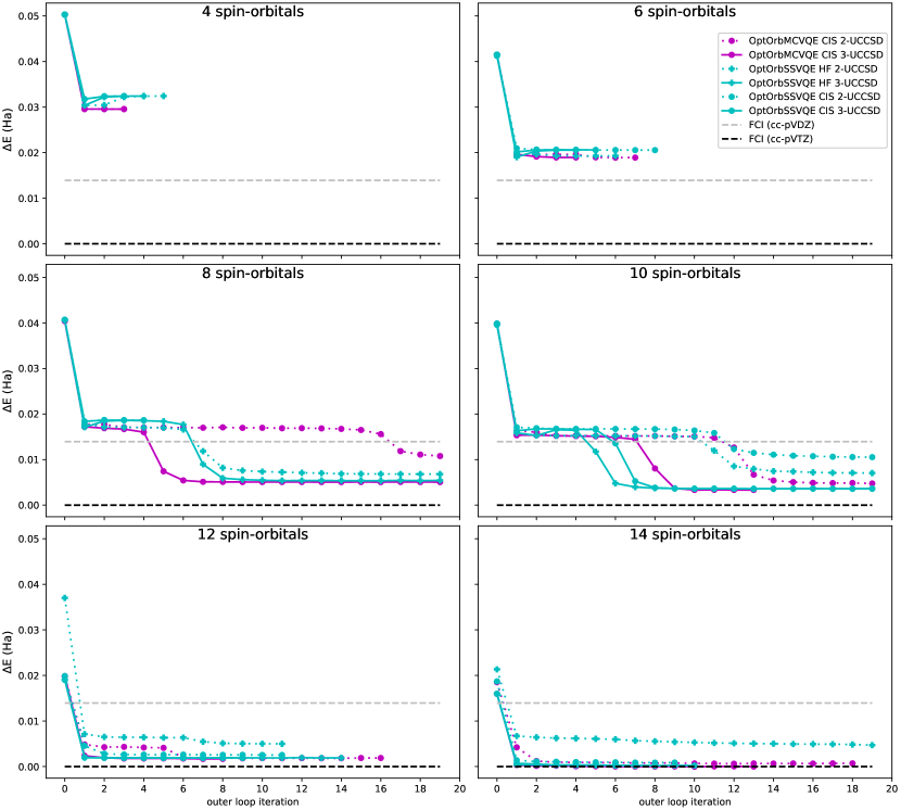
Figure 1: Convergence of orbital optimization methods for $\ch{H_{2}}$ using various numbers of spin-orbitals (taken from the cc-pVQZ basis) as a function of the outer loop iteration. $\Delta E$ is the difference between the average energy and that of FCI in the cc-pVTZ basis (56 spin-orbitals).

It is evident that orbital optimization has the potential to achieve more accurate average energies than FCI in the cc-pVDZ basis (20 spin-orbitals) and can even approach cc-pVTZ quality values, but this highly depends on the choice of eigensolver, ansatz, and number of optimized spin-orbitals. A minimum of 8 spin-orbitals are needed to achieve a higher accuracy than cc-pVDZ. At this point, OptOrbMCVQE can do this for both 2 and 3-UCCSD, although OptOrbSSVQE cannot. Using 10 spin-orbitals, both eigensolvers surpass cc-pVDZ for both 2 and 3-UCCSD, although MCVQE offers roughly a 5 milli-Hartree improvement over SSVQE for 2-UCCSD. When 3-UCCSD is used, MCVQE offers a measurable but negligible improvement over SSVQE. At 14 spin-orbitals, cc-pVTZ quality results are achievable. Also notable is the effect that increasing the active space has on not only the quality of convergence, but its rate of convergence. Note that for 8 and 10 spin-orbitals, the convergence appears to plateau, hovering just above cc-pVDZ accuracy for several iterations before rapidly surpassing it. This behavior is not present at 12 and 14 spin-obitals, with the energy quickly converging to near or at cc-pVTZ accuracy for the majority of tests run. As a sidenote, we note that the 14 spin-orbital tests using 3-UCCSD with a CIS initialization were stopped manually at iterations 10 and 13 for SSVQE and MCVQE, respectively as the runtime for these simulations proved to be the longest among these tests. However, we note that given that nearly all of the energy convergence occurred within the first 2 or 3 iterations, allowing the simulations to continue would likely not have resulted in further improvement.

4.2 H4

We now present the results for H4, a toy system comprised of four hydrogen atoms arranged in a square with a nearest-neighbor distance of 1.23 Å. The starting basis set is cc-pVQZ (240 spin-orbitals) and an active space of 8 optimized spin-orbitals is used. Both 2 and 3-UCCSD are tested as ansatzes and both CIS and CISD are tested as initializations. SSVQE is additionally tested using the Hartree-Fock initialization. The results are given in Fig. 2.

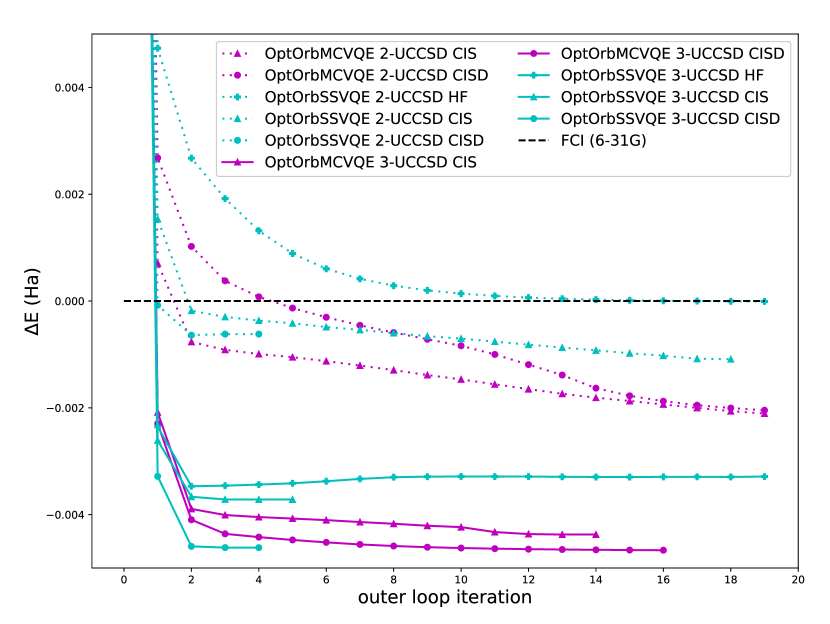
Figure 2: Convergence of orbital optimization methods for $\ch{H_{4}}$ using 8 optimized spin-orbitals (taken from the cc-pVQZ basis) as a function of the outer loop iteration. $\Delta E$ is the difference between the average energy and that of FCI in the 6-31G basis (16 spin-orbitals).

We can see that for this system, orbital optimization can be used to achieve a more accurate average energy than the 6-31G basis (16 spin-orbitals), despite the fact that it is utilizing half the number of spin-orbitals. Convergence approaching FCI cc-pVDZ (40 spin-orbitals) accuracy was not observed in our testing. Between the three different algorithmic choices considered (the eigensolver, the initialization, and the ansatz), increasing the ansatz expressiveness from 2-UCCSD to 3-UCCSD had the most significant effect on the converged accuracy. Changing the initialization from CIS to CISD offered a clear improvement when used with the 3-UCCSD ansatz, however the same is not true for 2-UCCSD. With 2-UCCSD, OptOrbSSVQE using CISD converges quickly to a local minimum, whereas OptOrbSSVQE using CIS converges (albeit comparatively slowly) to a more accurate average energy. The final converged values for OptOrbMCVQE are similar between CIS and CISD when using 2-UCCSD. Note also that for instances using the same ansatz and initialization, using MCVQE as the eigensolver typically offers an improvement over SSVQE. The one exception to this is using CISD with 3-UCCSD, where the difference between these two converged values is negligible.

4.3 LiH

We now present the results for the first two energy levels of LiH at the near-equilibrium interatomic distance of 1.595 Å. The starting basis set is cc-pVTZ (88 spin-orbitals) and an active space of 12 optimized spin-orbitals is used. Both 1 and 2-UCCSD are used to assess the effect of ansatz expressiveness. CIS and CISD initializations are tested for MCVQE whereas SSVQE additionally tests the Hartree-Fock initialization. The results are shown in Fig. 3.

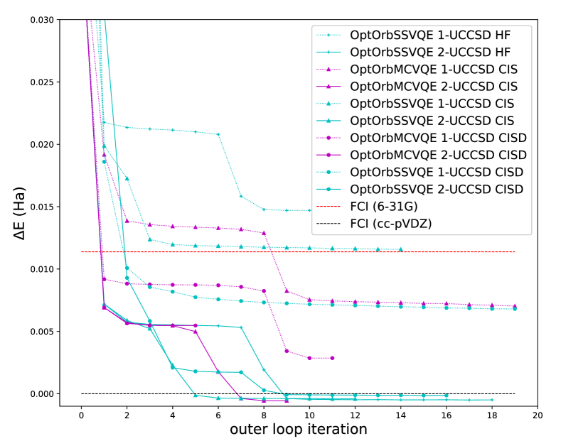
Figure 3: Convergence of orbital optimization methods for $\ch{LiH}$ using 12 optimized spin-orbitals as a function of the outer loop iteration. $\Delta E$ is the difference between the average energy and that of FCI in the cc-pVDZ basis (36 spin-orbitals).

The most notable feature of this plot is that orbital-optimized solvers can achieve more accurate results than FCI using much larger basis sets. For example, most tests run for this system outperform FCI 6-31G (22 spin-orbitals) while using only 12 spin-orbitals. Depending on the choice of solver, ansatz, and initialization, some instances also outperform FCI cc-pVDZ (36 spin-orbitals). The second notable feature is that ansatz expressiveness (typically) has a greater influence on the final accuracy than the choice of initialization. The 1 and 2-UCCSD tests almost form two cleanly separated accuracy tiers, except for OptOrbMCVQE using 1-UCCSD with a CISD initialization, which achieves a higher accuracy than MCVQE using CISD with 2-UCCSD. The choice of initialization has a greater impact when the less expressive 1-UCCSD ansatz is used and has little impact when the ansatz is sufficiently expressive to approximate the solution states well. The third notable feature is that OptOrbMCVQE typically outperforms OptOrbSSVQE when using the same ansatz and initialization, with the one exception to this being when CISD and 2-UCCSD are used. This effect is most noticeable when the less expressive 1-UCCSD ansatz is used.

4.4 BeH2

We now present the results for the first two energy levels of BeH2 with a linear geometry at the near-equilibrium Be-H distance of 1.3264Å. We find the full system with 14 spin-orbitals and 6 electrons to be intractable for our computational budget, so we freeze two electrons in the Hartree-Fock orbitals with the lowest energy and compare the active space energy against that of FCI using the same frozen core approximation. Because we do not wish for the quality of the frozen core approximation across different basis sets to influence the comparison against FCI values, here we will only compare the orbital optimized results starting with the cc-pVQZ basis with an active space of 12 spin-orbitals against FCI in the cc-pVQZ basis using an active space of 228 spin-orbitals. Because of the wide disparity in active space size, we do not expect the orbital optimized tests to approach chemical accuracy compared to FCI, however we may still gain some insight as to what portion of the full basis set energy is attainable using a small active space and what kind of improvement orbital optimization offers over a naive approach which chooses a fixed active space based on Hartree-Fock orbital energies. These results are given in Fig. 4.

Figure 4: Convergence of orbital optimization methods for $\ch{BeH2}$ using 12 optimized spin-orbitals as a function of the outer loop iteration. $\Delta E$ is the difference between the average energy and that of FCI in the cc-pVTZ basis.

5 Discussion and Conclusions

In this paper we have proposed an orbital optimization scheme which uses a state-averaged approach to compute excited states of electronic structure Hamiltonians. We have shown that this method can achieve more accurate results than FCI using much larger fixed basis sets. We have also investigated the effects of the choice of quantum eigensolver, ansatz expressiveness, and state initialization. While exceptions to these trends can be found in our results, we can make the following general observations:

• Increasing the ansatz expressiveness offers the most significant effect among these factors.

• MCVQE often offers an improvement in accuracy over SSVQE for lower ansatz expressiveness. When higher expressiveness is used, the difference is often less significant.

• CIS initializations often offer an improvement over Hartree-Fock initializations, however the advantage of using CISD over CIS is unclear. There are several instances of CISD initialized tests achieving a lower accuracy than their CIS (and even Hartree-Fock) counterparts.

The first of these is not surprising. The ansatz expressiveness is what primarily determines the variational flexibility of the quantum eigensolver at each outer loop iteration. The second observation can be explained by noting that for a given initialization and ansatz, the solution space of SSVQE is more restricted than MCVQE. The solution space of SSVQE with unequal weights consists of the low-lying eigenvectors themselves, whereas the solution space of MCVQE consists of the subspace spanned by the low-lying eigenvectors. MCVQE utilizes a post-processing step involving a low-dimensional diagonalization problem in this subspace. This additional variational flexibility may ease the convergence process and allow it to partially compensate for an insufficiently expressive ansatz. The third point, while less easily explained than the other two, can be conjectured about. While the initialization does have an effect on ansatz expressiveness as it determines which excitation operators in the UCCSD ansatz act non-trivially, is not as variationally flexible as the parameterized ansatz itself is. Furthermore, this state is computed in the initial basis set guess, which is usually low-quality compared to the optimized basis set. Thus there is no guarantee that CISD computed in this initial basis will continue to be advantageous over CIS for successive basis set rotations. This is less likely to be the case when compared to the Hartree-Fock initial state, which consists of only one Slater determinant and remains the same in the Jordan-Wigner qubit encoding for all basis sets.

One compelling and well-motivated extension of this work would be to take a state-specific orbital optimization approach rather than a state-averaged one. State-specific orbital optimization (as the name implies) optimizes a different basis set for each excited state individually rather than optimizing one basis set for an ensemble of excited states by minimizing its average energy. State-specific orbital optimization has been developed in the context of classical orbital optimization algorithms ³³, however this particular method relies on a full CI expansion of the wavefunction at every outer loop iteration. In the quantum computing setting, such an explicit wavefunction expansion (as opposed to the expectation value of observables used here) would involve exponentially costly tomography and classical storage. These CI wavefunction expansions are used to compute the overlap of two different excited states in two different basis sets and uses them to enforce their orthogonality. In the quantum computing setting, one would have to develop a method which can compute these overlaps without access to CI expansions or which does not require overlaps at all. This is an interesting problem and will be a direction of future investigation.

The work of JB and JL are supported by the US National Science Foundation under awards CHE-2037263 and DMS-2309378. YL is supported in part by the National Natural Science Foundation of China (12271109) and Shanghai Pilot Program for Basic Research - Fudan University 21TQ1400100 (22TQ017).

Appendix A Excited States Initializations and Ansatz Expressiveness

Here we test the effects of various initialization choices and levels of ansatz expressiveness on the convergence of MCVQE and SSVQE in a fixed minimal basis. These tests serve to illustrate our motivation for our particular choices in the orbital optimized tests in Section 4 of the main text. By “initialization” we mean the choice of non-parameterized subcircuit prepended to the parameterized ansatz. The ansatz parameters themselves are initialized to zero as this corresponds to the identity subcircuit. Thus, this allows us to explore various chemically motivated initializations. MCVQE is tested with configuration interaction singles (CIS) and configuration interaction singles and doubles (CISD) state initializations. SSVQE is tested with CIS and CISD as well as an “excited Hartree-Fock” initialization used in a previous study by the authors. ³¹. This initialization applies single-particle fermionic excitations to the Hartree-Fock state and chooses the resulting Slater determinants with the lowest energy to initialize the circuit. Such states are orthogonal and can thus be used with both MCVQE and SSVQE. The ansatz expressiveness is varied by varying the number of times the base UCCSD circuit pattern is repeated, where we denote the circuit consisting of $n$ UCCSD repetitions as $n$-UCCSD.

Table 1 shows the final average energy accuracy for the first three states of H4 at a nearest neighbor distance of 1.23 Å for various choices of eigensolver, state initialization, and UCCSD expressiveness. We can see that Hartree-Fock and CIS initializations fail to produce an accuracy greater than $10^{-2}$ Ha for any eigensolver or level of ansatz expressiveness. Furthermore, increasing the ansatz expressiveness offers no meaningful improvement for these initializations. On the other hand, the CISD initialization offers the ability to achieve greater than chemical accuracy. With 2-UCCSD, both eigensolvers fall just short of chemical accuracy, but increasing the ansatz to 3 and 4-UCCSD offers further improvements. Thus, we can see that there is motivation for developing circuits which correspond to CISD states.

Eigensolver	Initialization	UCCSD Repetitions
		1-rep	2-rep	3-rep	4-rep
MCVQE	CIS	$4.25\times 10^{-2}$	$3.85\times 10^{-2}$	$3.70\times 10^{-2}$	$3.70\times 10^{-2}$
MCVQE	CISD	$5.16\times 10^{-3}$	$2.16\times 10^{-3}$	$2.53\times 10^{-4}$	$3.73\times 10^{-8}$
SSVQE	HF	$5.78\times 10^{-2}$	$4.67\times 10^{-2}$	$3.70\times 10^{-2}$	$3.70\times 10^{-2}$
SSVQE	CIS	$4.26\times 10^{-2}$	$3.81\times 10^{-2}$	$3.70\times 10^{-2}$	$3.70\times 10^{-2}$
SSVQE	CISD	$5.41\times 10^{-3}$	$2.45\times 10^{-3}$	$1.56\times 10^{-4}$	$3.67\times 10^{-8}$

Table 1: The final accuracy of the average energy for H4 for given choices of eigensolver, initialization, and UCCSD ansatz expressiveness.

We now compare the speed of convergence between MCVQE and SSVQE for the four test instances in Fig. 5 which were able to surpass chemical accuracy. Fig. 5 plots the state-averaged energy accuracy as a function of the number of objective function evaluations. We can see that for all four instances, the state-averaged energy plateaus for many iterations before escaping and converging to (or closer to) the global minimum. This is consistent with previous studies which include SSVQE by the authors ³¹. Notably, MCVQE is less prone to this issue.

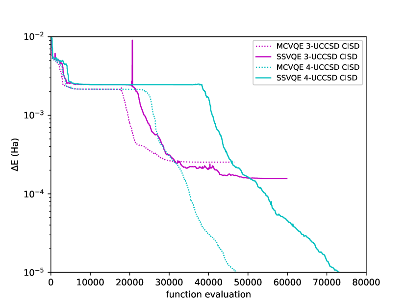
Figure 5: Convergence of the state-averaged energy accuracy ($\Delta E$)

Appendix B CIS State Preparation

Here we give an example of how configuration interaction singles (CIS) states can be prepared as a quantum circuit on a quantum computer using Givens rotations. It was proven that Givens rotations form a universal set of gates for chemically-motivated statevectors ⁴². The authors accomplish this constructively by giving a procedure for preparing an arbitrary state using Givens rotations controlled on the states of multiple qubits. They comment that for particular classes of states the resources involved may be reduced by controlling the rotation only on certain qubit subsets. What remains to be done is to work out the details of how to apply this idea to specific classes of CI statevectors (CIS, CISD, CISDT, ect…) in a way that is as gate-efficient as possible. Here we give an example of how both dense and sparse CIS statevectors can be mapped to quantum circuits using Givens rotations.

We briefly note that the CIS state preparation circuit outlined in the MCVQE proposal paper ³⁰ assumes a particular encoding where the reference state from which electrons are being excited is encoded as the "all-zero" state $\ket{00...0}$ where the qubit registers encode the occupation number of orbitals unoccupied in the reference state, but not those occupied in the reference state. Thus, the singly-excited wavefunction components contain no information about the particular Hartree-Fock occupied orbital from which the electron was excited. Here we seek a CIS state preparation circuit in the Jordan-Wigner encoding where the reference state is the Hartree-Fock state and the occupation number of orbitals occupied in this state are included for all wavefunction components. Thus, each singly-excited wavefunction component does contain information about the occupied Hartree-Fock orbital from which the electron was excited.

The matrix representation of a Givens rotation involving qubits $n$ and $m$ with angle $\theta$ is given by ⁴²:

$$G_{nm}(\theta)=\begin{pmatrix}1&0&0&0\\ 0&\cos{\theta}&-\sin{\theta}&0\\ 0&\sin{\theta}&\cos{\theta}&0\\ 0&0&0&1\end{pmatrix}$$ (10)

where the basis ordering is: $\ket{0}_{m}\ket{0}_{n}$, $\ket{0}_{m}\ket{1}_{n}$, $\ket{1}_{m}\ket{0}_{n}$, $\ket{1}_{m}\ket{1}_{n}$. or notational convenience, we will often omit the subscript $n$ and $m$ labels on qubit registers. We can also make use of Givens rotations controlled on the state of a target qubit $t$, which we denote by $C_{t}G_{nm}(\theta)$. This gate can be represented as:

$$C_{t}G_{nm}(\theta) =\ket{0}\bra{0}_{t}\otimes\ket{\psi}\bra{\psi}_{mn}$$ (11)

$$+\ket{1}\bra{1}_{t}\otimes G_{nm}(\theta)\ket{\psi}\bra{\psi}_{mn}.$$ (12)

We also note that we adopt the convention of Qiskit where in the Jordan-Wigner encoding, the qubits are ordered according to spin and Hartree-Fock energy. Orbitals with the same spin are ordered from right to left in ascending Hartree-Fock energy. Thus, the relevant action of a Givens rotation is:

$$G_{nm}(\theta)\ket{01}=\cos(\theta)\ket{01}+\sin(\theta)\ket{10}$$ (13)

We do not have to consider the action of Givens rotations on the state $\ket{10}$ as we are only interested in exciting particles to orbitals of higher energies from lower ones. The circuit notation for the single-excitation Givens rotation is given by ⁴²:

$$\Qcircuit@C=1em@R=1em{\lstick{\ket{0}}&\gate{G}\qw\\ \lstick{\ket{1}}\gate{G}\qwx\qw\\ }$$ (14)

We want to construct a circuit from Givens rotations which produces the state:

$$\ket{\mathrm{CIS}}=C_{\mathrm{HF}}\ket{\mathrm{HF}}+\sum_{p\in\mathcal{O}_{\mathrm{HF}},q\in\mathcal{U}_{\mathrm{HF}}}C_{p}^{q}\ket{\phi_{q}\leftarrow\phi_{p}}$$ (15)

where $\ket{\phi_{q}\leftarrow\phi_{p}}$ means the computational basis state produced by exciting an electron from orbital $\phi_{p}$ to orbital $\phi_{q}$ from the Hartree-Fock ground state. $\mathcal{O}_{\mathrm{HF}}$ and $\mathcal{U}_{\mathrm{HF}}$ denote the set of orbitals occupied and unoccupied in the Hartree-Fock state, respectively. We can solve for the coefficients $C_{p}^{q}$ classically then set them equal to the parameterized coefficients of the wavefunction expansion produced by a circuit comprised of Givens rotations. This produces a set of equations which can be solved to find the Givens angles which produce the circuit that prepares arbitrary CIS states.

B.1 Example 1: 3 particles, 6 spin-orbitals

We now give an example for the particular case where we want to generate the CIS wavefunction with 6 spin-orbitals and 3 particles, where all possible single-particle excitations are considered. The circuit for accomplishing this is given by:

$$\Qcircuit@C=1em@R=1em{\lstick{a\ket{1}}&\qw\qw\qw\targ\ctrl{3}\ctrl{2}\ctrl{1}\targ\ctrl{3}\ctrl{2}\ctrl{1}\targ\ctrl{4}\targ\targ\targ\qw\\ \lstick{q_{5}\ket{0}}\qw\qw\gate{G}\qw\qw\qw\gate{G}\qw\qw\qw\gate{G}\qw\qw\qw\qw\qw\qw\\ \lstick{q_{4}\ket{0}}\qw\gate{G}\gate{G}\qwx\qw\qw\gate{G}\gate{G}\qwx\qw\qw\gate{G}\gate{G}\qwx\qw\qw\qw\qw\qw\qw\\ \lstick{q_{3}\ket{0}}\gate{G}\gate{G}\qwx\qw\qw\gate{G}\gate{G}\qwx\qw\qw\gate{G}\gate{G}\qwx\qw\qw\qw\qw\qw\qw\qw\\ \lstick{q_{2}\ket{1}}\gate{G}\qwx\qw\qw\ctrlo{-4}\qw\qwx\qw\qw\qw\qw\qw\qwx\qw\qw\qw\gate{P}\qw\qw\ctrl{-4}\qw\\ \lstick{q_{1}\ket{1}}\qw\qw\qw\qw\gate{G}\qwx\qw\qw\ctrlo{-5}\qw\qwx\qw\qw\qw\qw\qw\ctrl{-5}\qw\qw\\ \lstick{q_{0}\ket{1}}\qw\qw\qw\qw\qw\qw\qw\qw\gate{G}\qwx\qw\qw\ctrlo{-6}\qw\ctrl{-6}\qw\qw\qw\\ }$$

where the register labelled as $a$ is an ancilla qubit and those labelled as $q_{i}$ are data qubits used to store the CIS state. CNOT gates with an open dot instead of the typical filled dot denote a CNOT gate where the NOT operation is controlled on the target qubit being in the state $\ket{0}$ instead of $\ket{1}$. Although it is not explicitly given in the circuit due to space constraints, each Givens rotation has its own parameter. The controlled phase gate $P$ (implicitly $P(\lambda))$ is given in matrix form by:

$$P(\lambda)=\begin{pmatrix}1&0&0&0\\ 0&1&0&0\\ 0&0&1&0\\ 0&0&0&e^{i\lambda}\end{pmatrix}$$

where the columns and rows are ordered as: $\ket{00},\ket{01},\ket{10},\ket{11}$. We will see later that we only need $\lambda$ to be $0$ or $\pi$. $\lambda=0$ corresponds to a 2-qubit identity gate, in which case we could omit this gate entirely, whereas $\lambda=\pi$ corresponds to a controlled-Z gate. We denote this gate as $P$ in order to keep full generality. The purpose of the final sequence of CNOT gates is to disentangle the ancilla qubit from the data qubits, putting the final state in the form $\ket{\mathrm{CIS}}\otimes\ket{0}$. Not applying this sequence of CNOTs results in a state of the form: $C_{\mathrm{HF}}\ket{\mathrm{HF}}\ket{1}+\ket{singly-excited-subspace}\ket{0}$. From a tomography perspective, this CNOT sequence is not strictly speaking necessary as taking the partial trace over the ancilla subspace results in the same state, but it simplifies wavefunction expansion notation. The final state of the data qubits is given by:

$$\begin{split}\ket{\mathrm{CIS}}=&e^{i\lambda}\cos{\theta^{3}_{2}}\cos{\theta^{3}_{1}}\cos{\theta^{3}_{0}}\ket{000111}\\ &+\cos{\theta^{3}_{2}}\cos{\theta^{3}_{1}}\sin{\theta^{3}_{0}}\cos{\theta^{4}_{0}}\ket{001110}\\ &+\cos{\theta^{3}_{2}}\cos{\theta^{3}_{1}}\sin{\theta^{3}_{0}}\sin{\theta^{4}_{0}}\cos{\theta^{5}_{0}}\ket{010110}\\ &+\cos{\theta^{3}_{2}}\cos{\theta^{3}_{1}}\sin{\theta^{3}_{0}}\sin{\theta^{4}_{0}}\sin{\theta^{5}_{0}}\ket{100110}\\ &\\ &+\cos{\theta^{3}_{2}}\sin{\theta^{3}_{1}}\cos{\theta^{4}_{1}}\ket{001101}\\ &+\cos{\theta^{3}_{2}}\sin{\theta^{3}_{1}}\sin{\theta^{4}_{1}}\cos{\theta^{5}_{1}}\ket{010101}\\ &+\cos{\theta^{3}_{2}}\sin{\theta^{3}_{1}}\sin{\theta^{4}_{1}}\sin{\theta^{5}_{1}}\ket{100101}\\ &\\ &+\sin{\theta^{3}_{2}}\cos{\theta^{4}_{2}}\ket{001011}\\ &+\sin{\theta^{3}_{2}}\sin{\theta^{4}_{2}}\cos{\theta^{5}_{2}}\ket{010011}\\ &+\sin{\theta^{3}_{2}}\sin{\theta^{4}_{2}}\sin{\theta^{5}_{2}}\ket{100011}.\\ \end{split}$$ (16)

We denote the angle which first adds the component $\ket{\phi_{q}\leftarrow\phi_{p}}$ to the overall wavefunction as $\theta^{q}_{p}$. By setting these coefficients equal to those of the CI wavefunction expansion given in Eq. 15, we arrive at the following set of equations:

$$\begin{split}&e^{i\lambda}\cos{\theta^{3}_{2}}\cos{\theta^{3}_{1}}\cos{\theta^{3}_{0}}=C_{\mathrm{HF}}\\ &\cos{\theta^{3}_{2}}\cos{\theta^{3}_{1}}\sin{\theta^{3}_{0}}\cos{\theta^{4}_{0}}=C^{3}_{0}\\ &\cos{\theta^{3}_{2}}\cos{\theta^{3}_{1}}\sin{\theta^{3}_{0}}\sin{\theta^{4}_{0}}\cos{\theta^{5}_{0}}=C^{4}_{0}\\ &\cos{\theta^{3}_{2}}\cos{\theta^{3}_{1}}\sin{\theta^{3}_{0}}\sin{\theta^{4}_{0}}\sin{\theta^{5}_{0}}=C^{5}_{0}\\ &\\ &\cos{\theta^{3}_{2}}\sin{\theta^{3}_{1}}\cos{\theta^{4}_{1}}=C^{3}_{1}\\ &\cos{\theta^{3}_{2}}\sin{\theta^{3}_{1}}\sin{\theta^{4}_{1}}\cos{\theta^{5}_{1}}=C^{4}_{1}\\ &\cos{\theta^{3}_{2}}\sin{\theta^{3}_{1}}\sin{\theta^{4}_{1}}\sin{\theta^{5}_{1}}=C^{5}_{1}\\ &\\ &\sin{\theta^{3}_{2}}\cos{\theta^{4}_{2}}=C^{3}_{2}\\ &\sin{\theta^{3}_{2}}\sin{\theta^{4}_{2}}\cos{\theta^{5}_{2}}=C^{4}_{2}\\ &\sin{\theta^{3}_{2}}\sin{\theta^{4}_{2}}\sin{\theta^{5}_{2}}=C^{5}_{2}.\\ \end{split}$$ (17)

The recursive structure of this circuit allows us to solve for all of these parameters analytically in a recursive way. We can partition these 10 equations into 3 blocks of 3 equations and one block with one equation according to the occupied Hartree-Fock orbital from which the excitations are generated. We start with $p=2$ and solve for $\theta^{5}_{2}$, $\theta^{4}_{2}$, and $\theta^{3}_{2}$ in that order. This has the solution:

$$\begin{split}&\theta^{5}_{2}=\arctan{\left(\frac{C^{5}_{2}}{C^{4}_{2}}\right)}\\ &\theta^{4}_{2}=\arctan{\left(\frac{1}{\cos{\theta^{5}_{2}}}\frac{C^{4}_{2}}{C^{3}_{2}}\right)}\\ &\theta^{3}_{2}=\arcsin{\left(\frac{C^{3}_{2}}{\cos{\theta^{4}_{2}}}\right)}.\\ \end{split}$$ (18)

The equations corresponding to $p=1$ are the same in structure to those of $p=2$, except that the left hand side is multiplied by a constant factor of $\cos{\theta^{3}_{2}}$, a quantity that we solved for in the $p=2$ equations. We define $\alpha_{2}=\cos{\theta^{3}_{2}}$ and divide both sides of these equations by $\alpha_{2}$. We arrive at a second set of solutions:

$$\begin{split}&\theta^{5}_{1}=\arctan{\left(\frac{C^{5}_{1}}{C^{4}_{1}}\right)}\\ &\theta^{4}_{1}=\arctan{\left(\frac{1}{\cos(\theta^{5}_{1})}\frac{C^{4}_{1}}{C^{3}_{1}}\right)}\\ &\theta^{3}_{1}=\arcsin{\left(\frac{1}{\alpha_{2}}\frac{C^{3}_{1}}{\cos(\theta^{4}_{1})}\right)}.\\ \end{split}$$ (19)

The $p=0$ block of equations also has the same form, but the left side is multiplied by a factor of $\alpha_{1}\alpha_{2}=\cos{\theta^{3}_{1}}\cos{\theta^{3}_{2}}$. We divide by sides of each equation in this block by $\alpha_{1}\alpha_{2}$ and arrive at the solution for this third block:

$$\begin{split}&\theta^{5}_{0}=\arctan{\left(\frac{C^{5}_{0}}{C^{4}_{0}}\right)}\\ &\theta^{4}_{0}=\arctan{\left(\frac{1}{\cos{\theta^{5}_{0}}}\frac{C^{4}_{0}}{C^{3}_{0}}\right)}\\ &\theta^{3}_{0}=\arcsin{\left(\frac{1}{\alpha_{1}\alpha_{2}}\frac{C^{3}_{0}}{\cos{\theta^{4}_{0}}}\right)}.\\ \end{split}$$ (20)

This leaves only the parameter $\lambda$ for which to solve. The magnitude of $C_{\mathrm{HF}}$ will match that of $\alpha_{2}\alpha_{1}\alpha_{0}$ due to the normalization condition, but the two may differ by a factor of either $+1$ or $-1$. The parameter $\lambda$ will determine this phase. If the phase of the two quantities match, then $\lambda=0$ and the phase gate can be omitted entirely. If the two differ by a phase of $-1$, then $\lambda=\pi$.

B.2 Example 2: Sparse 2 Particles, 6 Spin-Orbitals

The previous example dealt with the particular case of 3 particles and 6 spin-orbitals where every single-particle excitation from any occupied Hartree-Fock orbital is possible. We now give an example for a different number of particles and spin-orbitals for the case where the CIS wavefunction is sparse and some of the coefficients are zero. This demonstrates that we can also generate approximate CIS wavefunctions at lower circuit depth in a straightforward, systematic way by omitting certain excitations if their CI coefficients are below a specified threshold.

Here we suppose that we are preparing a CIS state of a system with 2 particles and 6 spin-orbitals, where $\phi_{1}$ can only be excited to $\{\phi_{2}$, $\phi_{5}\}$ and $\phi_{0}$ can only be excited to $\phi_{4}$. The circuit for doing so is given by:

$$\Qcircuit@C=1em@R=1em{\lstick{a\ket{1}}&\qw\qw\targ\ctrl{2}\targ\ctrl{5}\targ\targ\qw\\ \lstick{q_{5}\ket{0}}\qw\gate{G}\qw\qw\qw\qw\qw\qw\qw\\ \lstick{q_{4}\ket{0}}\qw\qw\qwx\qw\gate{G}\qw\qw\qw\qw\qw\\ \lstick{q_{3}\ket{0}}\qw\qw\qwx\qw\qw\qwx\qw\qw\qw\qw\qw\\ \lstick{q_{2}\ket{0}}\gate{G}\gate{G}\qwx\qw\qw\qwx\qw\qw\qw\qw\qw\\ \lstick{q_{1}\ket{1}}\gate{G}\qwx\qw\ctrlo{-5}\qw\qwx\qw\gate{P}\qw\ctrl{-5}\qw\\ \lstick{q_{0}\ket{1}}\qw\qw\qw\gate{G}\qwx\ctrlo{-6}\qw\ctrl{-6}\qw\qw\\ }$$

This results in the data qubits being put in the state:

$$\begin{split}\ket{\mathrm{CIS}}=&e^{i\lambda}\cos{\theta^{2}_{1}}\cos{\theta^{4}_{0}}\ket{000011}\\ +&\cos{\theta^{2}_{1}}\sin{\theta^{4}_{0}}\ket{010010}\\ +&\sin{\theta^{2}_{1}}\sin{\theta^{5}_{1}}\ket{100001}\\ +&\sin{\theta^{2}_{1}}\cos{\theta^{5}_{1}}\ket{000101}\\ \end{split}$$ (21)

This leads to the set of equations:

$$\begin{split}e^{i\lambda}\cos{\theta^{2}_{1}}\cos{\theta^{4}_{0}}&=C_{\mathrm{HF}}\\ &\\ \cos{\theta^{2}_{1}}\sin{\theta^{4}_{0}}&=C^{4}_{0}\\ &\\ \sin{\theta^{2}_{1}}\cos{\theta^{5}_{1}}&=C^{2}_{1}\\ \sin{\theta^{2}_{1}}\sin{\theta^{5}_{1}}&=C^{5}_{1}\\ \end{split}$$ (22)

We solve for $\theta^{5}_{1}$, $\theta^{2}_{1}$, $\theta^{4}_{0}$, and $\lambda$ recursively in that order. The solution is given by:

$$\begin{split}&\theta^{5}_{1}=\arctan{\left(\frac{C^{5}_{1}}{C^{2}_{1}}\right)}\\ &\theta^{2}_{1}=\arcsin{\left(\frac{C^{2}_{1}}{\cos{\theta^{5}_{1}}}\right)}\\ &\theta^{4}_{0}=\arcsin{\left(\frac{C^{4}_{0}}{\alpha_{1}}\right)}\\ &e^{i\lambda}=\frac{C_{\mathrm{HF}}}{\alpha_{1}\alpha_{0}}\\ \end{split}$$ (23)

B.3 General Procedure

Based on the particular examples given, we can observe a general procedure for any number of particles and spin-orbitals. We first partition the spin-orbitals into two sets $\mathcal{O}_{\mathrm{HF}}$ and $\mathcal{U}_{\mathrm{HF}}$, the set of spin-orbitals occupied and unoccupied in the Hartree-Fock reference state, respectively. For each $\phi_{p}\in\mathcal{O}_{\mathrm{HF}}$, we generate an ordered set $L_{p}$ of orbitals $\phi_{q}\in\mathcal{U}_{\mathrm{HF}}$ for which the CI amplitude $C^{q}_{p}$ is not zero or is not below a desired truncation threshold. These orbitals are ordered in ascending Hartree-Fock energy. For every spin-orbital in each $L_{p}$, we map the orbital indices $q$ to new indices $n_{p}^{q}$. This is simply so that we may write down a general analytical expression for the gate sequence which reflects the fact we may not want or need the full, dense CI wavefunction. $n_{p}^{q}$ is the index of the list $L_{p}$ which was mapped from the original index of the spin-orbital $\phi_{q}$. e.g. the original set of unoccupied orbitals from which a particular occupied orbital may be given by $\{\phi_{3},\phi_{6},\phi_{8}\}$, but we map this ordered set to the list indices $\{0,1,2\}$.

The general sequence of gates is given by:

$$\begin{split}\ket{\mathrm{CIS}}=&\left[\prod_{\phi_{p}\in\mathcal{O}_{\mathrm{HF}}}\mathrm{CNOT}(a,p)\right]C_{a}P(\lambda)_{0}\\ &\times\prod_{\phi_{p}\in\mathcal{O}_{\mathrm{HF}}\setminus\{\phi_{0}\}}^{q_{max}-1}\left[X_{p}\mathrm{CNOT}(a,p)X_{p}\prod_{\phi_{q}\in L_{p}}C_{a}G_{n_{p}^{q},n_{p}^{q}+1}\right]\\ &\times X_{0}\mathrm{CNOT}(a,0)X_{0}\prod_{\phi_{q}\in L_{0}}^{q_{max}-1}G_{n_{0}^{q},n_{0}^{q}+1}(\theta^{q}_{0})\ket{\mathrm{HF}}\ket{1}_{a}\end{split}$$ (24)

The rightmost terms denote the fact that for the set of excitations from the first occupied spin-orbital, we do not have to apply the Givens rotations conditioned on the state of the ancilla qubit. Without loss of generality, we may take $\phi_{0}$ to be the orbital which has the longest list $L_{p}$ of possible excited orbitals. This will reduce the circuit depth as compiling controlled Givens rotations into a sequence of 1 and 2-qubit basis gates will in general be more expensive than regular Givens rotations. After this, we apply a NOT gate to the ancilla qubit conditioned on the state of the qubit from which we just generated excitations being $\ket{0}$. This marks all data qubit wavefunction components that are not the Hartree-Fock component so that future Givens rotations will not apply excitations to these components. We then repeat this with Givens rotations controlled on the state of the ancilla for all the other Hartree-Fock occupied orbitals. If there is an orbital for which there are no possible excitations, we simply skip it. We then apply a phase gate $P(\lambda)$ to any of the Hartree-Fock occupied orbitals conditioned on the state of the ancilla. This applies the relative phase $e^{i\lambda}$ to the Hartree-Fock component of the wavefunction. Finally, for each of the Hartree-Fock occupied orbitals, we apply a NOT gate controlled on the state of the ancilla. This disentangles the data qubits from the ancilla qubit so that the final result is a product state of these registers.

Finally, we give a general procedure for mapping the CI coefficients $C^{q}_{p}$ to the Givens rotation angles $\theta^{q}_{p}$. In order to do this, we temporarily re-index the CI coefficient indices in the same way that we did for the general circuit expression. For each $L_{p}$, we map the orbital indices $q\rightarrow n^{q}_{p}$. Here, $C^{n^{q}_{p}}_{p}$ is the re-indexed CI coefficient mapped from $C^{q}_{p}$ for list $L_{p}$. The sequence of steps for this procedure can be given by:

1. For each $\phi_{p}\in\mathcal{O}_{\mathrm{HF}}$ (In the corresponding order applied in the circuit):

   1. If length($L_{p}$) = 1:

      $$\theta^{n^{q}_{p}}_{p}=\arcsin{\left(\frac{C^{n^{q}_{p}}_{p}}{\prod_{p^{\prime}<p}\alpha_{p^{\prime}}}\right)}$$

   2. If length($L_{p}$) = 2:

      $$\begin{split}&\theta^{n^{q}_{p}=1}_{p}=\arctan{\left(\frac{C^{n^{q}_{p}=1}_{p}}{C^{n^{q}_{p}=0}_{p}}\right)}\\ &\theta^{n^{q}_{p}=0}_{p}=\arcsin{\left(\frac{1}{\prod_{p^{\prime}<p}\alpha_{p^{\prime}}}\frac{C^{n^{q}_{p}=0}}{\cos{\left(\theta_{p}^{n^{q}_{p}=0}\right)}}\right)}\end{split}$$

   3. If length($L_{p}$) > 2:

      $$\theta^{n^{q_{max}}_{p}}_{p} = \arctan{\left(\frac{C^{n^{q_{max}}_{p}}_{p}}{C^{n^{q_{max}}_{p}-1}_{p}}\right)}$$

      $$\theta^{n^{q_{max}}_{p}-1}_{p} = \arctan{\left(\frac{1}{\cos{\left(\theta^{n^{q_{max}}_{p}}_{p}\right)}}\frac{C^{n^{q_{max}}_{p}-1}_{p}}{C^{n^{q_{max}}_{p}-2}_{p}}\right)}$$

      $$\vdots$$

      $$\theta^{n^{q}_{p}}_{p} = \arctan{\left(\frac{1}{\cos{\left(\theta^{n^{q}_{p}+1}_{p}\right)}}\frac{C^{n^{q}_{p}}_{p}}{C^{n^{q}_{p}-1}_{p}}\right)}$$

      $$\vdots$$

      $$\theta^{n^{q}_{p}=0}_{p} = \arcsin{\left(\frac{1}{\prod_{p^{\prime}<p}\alpha_{p^{\prime}}}\frac{C^{n^{q}_{p}=0}}{\cos{\left(\theta_{p}^{n^{q}_{p}=0}\right)}}\right)}$$

2. Solve for $\lambda$:

   $$\lambda=\begin{cases}0,&\text{if}\ \frac{C_{\mathrm{HF}}}{\prod_{p}\alpha_{p}}=1\\ \pi,&\text{if}\ \frac{C_{\mathrm{HF}}}{\prod_{p}\alpha_{p}}=-1\end{cases}$$

Here, for the sake of notational convenience we define $\prod_{p^{\prime}<0}\alpha_{p^{\prime}}=1$.

References

- Helgaker et al. 2014 Helgaker, T.; Jorgensen, P.; Olsen, J. Molecular Electronic-Structure Theory; Wiley, 2014
- Kühn et al. 2019 Kühn, M.; Zanker, S.; Deglmann, P.; Marthaler, M. et al. Accuracy and Resource Estimations for Quantum Chemistry on a Near-Term Quantum Computer. J. Chem. Theory Comput. 2019, 15, 4764–4780
- Elfving et al. 2020 Elfving, V. E.; Broer, B. W.; Webber, M.; Gavartin, J. et al. How Will Quantum Computers Provide an Industrially Relevant Computational Advantage in Quantum Chemistry? 2020
- Gonthier et al. 2022 Gonthier, J. F.; Radin, M. D.; Buda, C.; Doskocil, E. J. et al. Measurements as a Roadblock to Near-Term Practical Quantum Advantage in Chemistry: Resource Analysis. Phys. Rev. Res. 2022, 4, 033154
- Kandala et al. 2017 Kandala, A.; Mezzacapo, A.; Temme, K.; Takita, M. et al. Hardware-Efficient Variational Quantum Eigensolver for Small Molecules and Quantum Magnets. Nature 2017, 549, 242–246
- Shen et al. 2017 Shen, Y.; Zhang, X.; Zhang, S.; Zhang, J.-N. et al. Quantum Implementation of the Unitary Coupled Cluster for Simulating Molecular Electronic Structure. Phys. Rev. A 2017, 95, 020501
- O’Malley et al. 2016 O’Malley, P. J. J.; Babbush, R.; Kivlichan, I. D.; Romero, J. et al. Scalable Quantum Simulation of Molecular Energies. Phys. Rev. X 2016, 6, 031007
- Ganzhorn et al. 2019 Ganzhorn, M.; Egger, D.; Barkoutsos, P.; Ollitrault, P. et al. Gate-Efficient Simulation of Molecular Eigenstates on a Quantum Computer. Phys. Rev. Appl. 2019, 11, 044092
- McArdle and Tew 2020 McArdle, S.; Tew, D. P. Improving the Accuracy of Quantum Computational Chemistry Using the Transcorrelated Method. 2020
- Sokolov et al. 2023 Sokolov, I. O.; Dobrautz, W.; Luo, H.; Alavi, A. et al. Orders of Magnitude Reduction in the Computational Overhead for Quantum Many-Body Problems on Quantum Computers via an Exact Transcorrelated Method. 2023, arXiv:2201.03049
- Motta et al. 2020 Motta, M.; Gujarati, T. P.; Rice, J. E.; Kumar, A. et al. Quantum Simulation of Electronic Structure with a Transcorrelated Hamiltonian: Improved Accuracy with a Smaller Footprint on the Quantum Computer. Phys. Chem. Chem. Phys. 2020, 22, 24270–24281
- Kumar et al. 2022 Kumar, A.; Asthana, A.; Masteran, C.; Valeev, E. F. et al. Quantum Simulation of Molecular Electronic States with a Transcorrelated Hamiltonian: Higher Accuracy with Fewer Qubits. J. Chem. Theory Comput. 2022, 18, 5312–5324
- Kong et al. 2012 Kong, L.; Bischoff, F. A.; Valeev, E. F. Explicitly Correlated R12/F12 Methods for Electronic Structure. Chem. Rev. 2012, 112, 75–107
- Kutzelnigg and Morgan 1992 Kutzelnigg, W.; Morgan, J. D., III Rates of Convergence of the Partial-wave Expansions of Atomic Correlation Energies. The Journal of Chemical Physics 1992, 96, 4484–4508
- Metcalf et al. 2020 Metcalf, M.; Bauman, N. P.; Kowalski, K.; de Jong, W. A. Resource-Efficient Chemistry on Quantum Computers with the Variational Quantum Eigensolver and the Double Unitary Coupled-Cluster Approach. J. Chem. Theory Comput. 2020, 16, 6165–6175
- Huang et al. 2022 Huang, R.; Li, C.; Evangelista, F. A. Leveraging Small Scale Quantum Computers with Unitarily Downfolded Hamiltonians. 2022
- Claudino et al. 2021 Claudino, D.; Peng, B.; Bauman, N. P.; Kowalski, K. et al. Improving the Accuracy and Efficiency of Quantum Connected Moments Expansions*. Quantum Sci. Technol. 2021, 6, 034012
- Bauman et al. 2019 Bauman, N. P.; Bylaska, E. J.; Krishnamoorthy, S.; Low, G. H. et al. Downfolding of Many-Body Hamiltonians Using Active-Space Models: Extension of the Sub-System Embedding Sub-Algebras Approach to Unitary Coupled Cluster Formalisms. The Journal of Chemical Physics 2019, 151, 014107
- Bauman et al. 2019 Bauman, N. P.; Low, G. H.; Kowalski, K. Quantum Simulations of Excited States with Active-Space Downfolded Hamiltonians. The Journal of Chemical Physics 2019, 151, 234114
- Bierman et al. 2023 Bierman, J.; Li, Y.; Lu, J. Improving the Accuracy of Variational Quantum Eigensolvers with Fewer Qubits Using Orbital Optimization. J. Chem. Theory Comput. 2023, 19, 790–798
- Omiya et al. 2022 Omiya, K.; Nakagawa, Y. O.; Koh, S.; Mizukami, W. et al. Analytical Energy Gradient for State-Averaged Orbital-Optimized Variational Quantum Eigensolvers and Its Application to a Photochemical Reaction. J. Chem. Theory Comput. 2022, 18, 741–748
- de Gracia Triviño et al. 2023 de Gracia Triviño, J. A.; Delcey, M. G.; Wendin, G. Complete Active Space Methods for NISQ Devices: The Importance of Canonical Orbital Optimization for Accuracy and Noise Resilience. J. Chem. Theory Comput. 2023,
- Mizukami et al. 2020 Mizukami, W.; Mitarai, K.; Nakagawa, Y. O.; Yamamoto, T. et al. Orbital Optimized Unitary Coupled Cluster Theory for Quantum Computer. Phys. Rev. Res. 2020, 2, 033421
- Li and Lu 2020 Li, Y.; Lu, J. Optimal Orbital Selection for Full Configuration Interaction (OptOrbFCI): Pursuing the Basis Set Limit under a Budget. J. Chem. Theory Comput. 2020, 16, 6207–6221
- Tilly et al. 2021 Tilly, J.; Sriluckshmy, P. V.; Patel, A.; Fontana, E. et al. Reduced Density Matrix Sampling: Self-consistent Embedding and Multiscale Electronic Structure on Current Generation Quantum Computers. Phys. Rev. Res. 2021, 3, 033230
- Yalouz et al. 2021 Yalouz, S.; Senjean, B.; Günther, J.; Buda, F. et al. A State-Averaged Orbital-Optimized Hybrid Quantum–Classical Algorithm for a Democratic Description of Ground and Excited States. Quantum Sci. Technol. 2021, 6, 024004
- Peruzzo et al. 2014 Peruzzo, A.; McClean, J.; Shadbolt, P.; Yung, M.-H. et al. A Variational Eigenvalue Solver on a Photonic Quantum Processor. Nat Commun 2014, 5, 4213
- Tilly et al. 2022 Tilly, J.; Chen, H.; Cao, S.; Picozzi, D. et al. The Variational Quantum Eigensolver: A Review of Methods and Best Practices. Physics Reports 2022, 986, 1–128
- Nakanishi et al. 2019 Nakanishi, K. M.; Mitarai, K.; Fujii, K. Subspace-Search Variational Quantum Eigensolver for Excited States. Phys. Rev. Res. 2019, 1, 033062
- Parrish et al. 2019 Parrish, R. M.; Hohenstein, E. G.; McMahon, P. L.; Martínez, T. J. Quantum Computation of Electronic Transitions Using a Variational Quantum Eigensolver. Phys. Rev. Lett. 2019, 122, 230401
- Bierman et al. 2022 Bierman, J.; Li, Y.; Lu, J. Quantum Orbital Minimization Method for Excited States Calculation on a Quantum Computer. J. Chem. Theory Comput. 2022, 18, 4674–4689
- Higgott et al. 2019 Higgott, O.; Wang, D.; Brierley, S. Variational Quantum Computation of Excited States. Quantum 2019, 3, 156
- Yalouz and Robert 2023 Yalouz, S.; Robert, V. Orthogonally Constrained Orbital Optimization: Assessing Changes of Optimal Orbitals for Orthogonal Multireference States. J. Chem. Theory Comput. 2023, 19, 1388–1392
- Wen and Yin 2013 Wen, Z.; Yin, W. A Feasible Method for Optimization with Orthogonality Constraints. Math. Program. 2013, 142, 397–434
- Gao et al. 2019 Gao, B.; Liu, X.; Yuan, Y.-x. Parallelizable Algorithms for Optimization Problems with Orthogonality Constraints. SIAM J. Sci. Comput. 2019, 41, A1949–A1983
- Zhang et al. 2014 Zhang, X.; Zhu, J.; Wen, Z.; Zhou, A. Gradient Type Optimization Methods For Electronic Structure Calculations. SIAM J. Sci. Comput. 2014, 36, C265–C289
- Huang et al. 2015 Huang, W.; Gallivan, K. A.; Absil, P.-A. A Broyden Class of Quasi-Newton Methods for Riemannian Optimization. SIAM J. Optim. 2015, 25, 1660–1685
- Gao et al. 2018 Gao, B.; Liu, X.; Chen, X.; Yuan, Y.-x. A New First-Order Algorithmic Framework for Optimization Problems with Orthogonality Constraints. SIAM J. Optim. 2018, 28, 302–332
- Qiskit contributors 2023 Qiskit contributors, Qiskit: An Open-source Framework for Quantum Computing. 2023
- Sun et al. 2018 Sun, Q.; Berkelbach, T. C.; Blunt, N. S.; Booth, G. H. et al. PySCF: The Python-based Simulations of Chemistry Framework. WIREs Computational Molecular Science 2018, 8, e1340
- Harris et al. 2020 Harris, C. R.; Millman, K. J.; van der Walt, S. J.; Gommers, R. et al. Array Programming with NumPy. Nature 2020, 585, 357–362
- Arrazola et al. 2022 Arrazola, J. M.; Matteo, O. D.; Quesada, N.; Jahangiri, S. et al. Universal Quantum Circuits for Quantum Chemistry. Quantum 2022, 6, 742
- Romero et al. 2018 Romero, J.; Babbush, R.; McClean, J. R.; Hempel, C. et al. Strategies for Quantum Computing Molecular Energies Using the Unitary Coupled Cluster Ansatz. Quantum Sci. Technol. 2018, 4, 014008
- Byrd et al. 1995 Byrd, R. H.; Lu, P.; Nocedal, J.; Zhu, C. A Limited Memory Algorithm for Bound Constrained Optimization. SIAM J. Sci. Comput. 1995, 16, 1190–1208
- Wang et al. 2019 Wang, Z.; Li, Y.; Lu, J. Coordinate Descent Full Configuration Interaction. J. Chem. Theory Comput. 2019, 15, 3558–3569