ZeroSwap: Data-driven Optimal Market Making in DeFi

Abstract.

Automated Market Makers (AMMs) are major centers of matching liquidity supply and demand in Decentralized Finance. Their functioning relies primarily on the presence of liquidity providers (LPs) incentivized to invest their assets into a liquidity pool. However, the prices at which a pooled asset is traded is often more stale than the prices on centralized and more liquid exchanges. This leads to the LPs suffering losses to arbitrage. This problem is addressed by adapting market prices to trader behavior, captured via the classical market microstructure model of Glosten and Milgrom. In this paper, we propose the first optimal Bayesian and the first model-free data-driven algorithm to optimally track the external price of the asset. The notion of optimality that we use enforces a zero-profit condition on the prices of the market maker, hence the name ZeroSwap. This ensures that the market maker balances losses to informed traders with profits from noise traders. The key property of our approach is the ability to estimate the external market price without the need for price oracles or loss oracles. Our theoretical guarantees on the performance of both these algorithms, ensuring the stability and convergence of their price recommendations, are of independent interest in the theory of reinforcement learning. We empirically demonstrate the robustness of our algorithms to changing market conditions.

1. Introduction

Market making is an essential service that is used to satisfy liquidity demand in any financial system. Efficient market making in traditional finance involves providing bid and ask quotes for an asset that are as close to each other as possible, while accurately reflecting the price of the asset on a limit order book and thus providing a slight profit to the market maker. This efficiency is achieved by using increasingly complex models for trader behavior (GLOSTEN198571, ; kyleModel, ; grossmanMiller, ) and then inferring the underlying hidden price from the observed trader behavior. These models have now become canonical knowledge in the domains of microeconomics and market microstructure.

More recently, the problem of market making has come to the forefront in Decentralized Finance. DeFi uses Automated Market Makers, specifically Constant Function Market Makers (CFMMs) (angeris2021constant, ), as an alternative to limit order books. This decreases the computational load required in satisfying trades, while also providing deep markets for infrequently traded tokens. Additionally, the liquidity required to satisfy trades is also provided in a decentralized manner by liquidity providers (LPs), who pool their tokens to help satisfy the liquidity demand.

Markets in DeFi come with a variety of differing characteristics. The main differences are along market depth (or liquidity), and price volatility. For instance, stablecoin trading volume ($\approx\$11.1$ trillion) recently surpassed that of the amount transacted via centralized services such as MasterCard and PayPal (stablecoin3, ). Some of the deepest markets in terms liquidity also happen to be those containing stablecoins (univ3, ). These markets also do not face much volatility, and their depth ensures that the price impact of retail trades is small. On the other hand, DeFi also has hundreds of tokens that do not trade frequently and hence need liquid markets. Because of lack of liquidity, such markets are volatile and the price is sensitive even to retail trades. In this work, we focus on the former type of DeFi market.

The main problem in a CFMM is to incentivize the LPs to pool their tokens. To do that, the CFMM needs to ensure they do not face losses on an average. However, it is common knowledge that LPs do indeed face various kinds of losses due to changing reserves (loesch2021impermanent, ) and their lack of information about the market conditions (milionis2022automated, ). In the current paper, we focus on mitigating the loss that arises due to this lack of information. In particular, CFMMs with static curves often lead to LPs suffering losses due to arbitrageurs. These losses are supposed to be compensated with the fees charged on each trade. They arise from the fact that the CFMM always provide tokens at a price that is stale compared to an external, more liquid market, which opens up an arbitrage opportunity.

This arbitrage loss can be quantified for a special case as loss-versus-rebalancing (LVR) (milionis2022automated, ), and persists even after the introduction of fees (milionis2023automated, ). For a general market maker that offers to sell and buy a risky asset at the ask and bid prices respectively, the arbitrage loss is specified with respect to the external true price of the asset. The arbitrageur does a buy trade when the external price exceeds the ask price and does a sell trade when it is below the bid price. The loss to the market maker can be quantified as the difference between the two prices times the amount of asset being traded.

In traditional finance, this arbitrage loss has been modeled as the adverse selection cost arising because of interaction with informed traders (traders that know the external price - same as arbitrageurs). An optimal market maker exactly balances this cost with the profits arising from interaction with uninformed traders (or noise traders). This condition for optimality was first proposed by Glosten and Milgrom (GLOSTEN198571, ). In DeFi, this classification of traders has been termed as toxic and non-toxic order flow corresponding to informed and uninformed trade respectively (nezlobinToxicity, ; crocToxicity, ).

For CFMMs, this loss also stems from the fact that it needs to incentivize a trader to truthfully indicate their belief about the price, via their trades. This implies that, to track the external price accurately, the CFMM ends up paying the informed traders, in return for their information. This fact is also apparent from the connection between CFMMs and information eliciting market scoring rules used in prediction markets (frongillo2023axiomatic, ).

Naively, the loss to arbitrageurs can be minimized by simply setting the marginal price to be equal to the external price. This would need access to a price oracle, and has indeed been tried in some market making protocols (dodoOracle, ). However, coupling a market maker to an oracle opens the door to frontrunning attacks (frontrunningOracles, ) and places trust in an external centralized entity (Eskandari_2021, ; oraclesProblem, ) that may itself be manipulated. To avoid this, the main constraint we impose is the absence of any access to oracles. The challenge is to infer the hidden price simply by observing the history of trades, in as sample-efficient manner as possible.

The current work formulates this challenge using the Glosten-Milgrom model of trader behaviour, which specifies the proportion of informed and uninformed traders, their sequential interaction with the market maker and the evolution of the external price. We further assume that the jumps in the hidden price happen on the same time scale as the trades, and that the jump sizes are limited, since we focus on liquid and less volatile markets such as those involving stablecoins. The objective of the market maker is to adaptively set the ask and bid prices so that the loss to arbitrageurs is as close to zero as possible, which is why we call the market maker ZeroSwap. The market maker turning a profit would be undesirable since this would allow a competitor to undercut its prices and take away their order flow. In other words, the market maker should quote an efficient and competitive market price, given only the information it has in form of the trading history. Keeping this objective in mind, we make the following key contributions:

Model-based Bayesian algorithm. When the parameters of the trader and price behaviour model are known, we provide a Bayesian algorithm to update the ask and bid prices. We theoretically guarantee that the bid-ask spread of this algorithm is stable in presence of trades, and converges to the external market price. We empirically demonstrate that the loss to the market maker using this algorithm is zero, and it can hence be used as a benchmark for an optimally efficient market maker (Section 4).

Model-free data-driven algorithm. When the model parameters are unknown, we design a randomized algorithm which depends only on the trade history visible to the market maker. We empirically demonstrate that it tracks the hidden external price even under rapidly changing market conditions, and incurs a similar loss as a market maker that has access to an oracle. We give a first-of-its-kind theoretical guarantee that maximizing the corresponding cumulative reward ensures that the external price is tracked by the market maker efficiently; this is of independent interest in the theory of reinforcement learning (Section 5).

On-chain implementation. The market-making logic driven by the reinforcement learning engine is straightforward to implement as a smart contract on a blockchain, but entirely impractical due to the associated gas fees. We specify how to implement ZeroSwap as an application-specific rollup, in the context of the Ethereum blockchain (Section 6). The actual implementation is on-going work and outside the scope of this paper.

2. Related work

In this section, we reprise relevant literature surrounding the problem formulated in this paper. Although the motivation of the problem stems from literature studying AMMs in DeFi, our formulation derives heavily from classical works in market microstructure. The data-driven algorithm we present is motivated from canonical reinforcement learning literature.

Automated Market Makers: Automated Market Makers, in their most popular form as Constant Function Market Makers (sokDex, ; mohanDexPrimer, ), have been known to incentivize trades that make prices consistent with an external, more liquid market (Angeris_2020, ). It is also known that doing this incurs a cost to the liquidity providers of the CFMMs, and a profit to the arbitrageurs (evans2021optimal, ; Heimbach_2022, ; tangri2023generalizing, ). This profit can be quantified as “loss-versus-rebalancing” in the case of a market maker with only arbitrageurs (informed traders) trading with it (milionis2022automated, ), and is seen to be proportional to external price volatility. Several works propose to capture this loss, either via an on-chain auction (mcmenamin2022diamonds, ) or using auction theory to generate a dynamic ask and bid price recommendation for an AMM (milionis2023myersonian, ). Another recent work (goyal2023finding, ) proposes an optimal curve for a CFMM based on the LP beliefs over prices, however, the work does not consider a dynamic model where the trader reacts based on the market maker setting their prices. Our work is related closest to (milionis2023myersonian, ), where a dynamic model of trading is indeed considered, and optimal ask and bid prices are derived. However, the price recommendations require the market maker to know underlying model parameters, and thus the solution is not model-free or data-driven. Additionally, we look at a competitive market maker, while (milionis2023myersonian, ) look at the monopolistic case. Data-driven reinforcement learning algorithms to adapt CFMMs have also been used in another recent work (churiwala2022qlammp, ), albeit the objective there is to control fee revenue and minimize the number of failed trades.

Optimal market making: The trader behavior model that we use derives from the Glosten-Milgrom model (GLOSTEN198571, ) used extensively in market microstructure literature, however we modify it to have a continuously changing external price. Several followup works (das2005learning, ; das2008adapting, ) derive optimal market making rules under a modified Glosten-Milgrom framework, but they assume that underlying model parameters are known, and that external price jumps are notified to the market maker. A more data-driven reinforcement learning approach is followed in (chan2001, ), but the reward function they assume contains direct information about the external hidden price, while we assume no price oracle access. Another thread of optimal market making in traditional market microstructure literature deals with inventory management (hoAndStoll, ; avellaneda2008, ) as opposed to the information asymmetry between traders and market makers. However, we seek to design a market maker that covers losses from information asymmetry as in the Glosten-Milgrom model, assuming no constraints on the inventory. The Glosten-Milgrom model has already been considered for AMMs in DeFi, albeit only for single trades (aoyagi2020LP, ; angeris2020does, ).

POMDPs and Q-Learning: Partially Observable Markov Decision Processes (POMDPs) are used to model decision making problems where an underlying state evolves in a Markovian manner, but is invisible to the agent. Q-learning (watkins1992q, ) is a standard model-free method that is guaranteed to learn an optimal decision making policy for Markov Decision Processes (MDPs). Here, the optimality is in terms of maximizing expected cumulative reward. We formulate the optimal market making problem as a POMDP. We then adapt the algorithm for the POMDP defined by our model, and design a reward that helps us achieve the goal of optimal market making.

3. Price and trader behaviour model

We now describe the framework used for modeling trader behavior in response to the evolution of a hidden price process and prices set by the market maker. We also state the objective that the market maker seeks to optimize, and provide the motivation behind it. The model and the objective are based on the canonical Glosten-Milgrom model (GLOSTEN198571, ) studied extensively in market microstructure literature. In this work, we consider a discrete time model indexed by $t$.

External price process: The external price process $p_{ext}^{t}$ of a risky asset is assumed to follow a discrete time random walk, where probability of a jump at any $t$ is given by $\sigma$. That is, we have

(1) $$p_{ext}^{t+1}=\begin{cases}p_{ext}^{t}+1\ \ &\mathrm{w.p.\ }\sigma/2\\ p_{ext}^{t}-1\ \ &\mathrm{w.p.\ }\sigma/2\\ p_{ext}^{t}\ \ &\mathrm{w.p.\ }1-\sigma\end{cases}$$

This process can represent either the price of the asset in a larger and much more liquid exchange, or some underlying “true” value of the asset. In either case, we assume that it is hidden from the market maker. We use the same notation ($\sigma$) as the continuous-time volatility for our jump probability since they both represent a qualitative measure of the change in the external price.

Market Maker: The market maker publishes an ask $p_{a}^{t}$ and a bid $p_{b}^{t}$ price in every time slot. Any trader can respectively buy and sell the asset at these prices.

Trade actions: We assume that the traders arrive at a constant rate of $\lambda$. This means that for time slots which are multiples of $1/\lambda$, a trader comes in to interact with the market maker by performing an action $d_{t}$. It can choose to either buy ($d_{t}=+1$), sell ($d_{t}=-1$) or do neither ($d_{t}=0$). What the trader chooses to do depends on what they believe the value of the external price is.

Trader behavior: We assume two types of traders - informed and uninformed. The informed trader is assumed to know the external price exactly, while the uninformed trader does not know it at all. The informed trader buys a unit quantity of asset if $p_{ext}^{t}>p_{a}^{t}$ and sells a unit quantity of asset if $p_{ext}^{t}<p_{b}^{t}$, thus acting as an arbitrageur between the market maker and the external market. The uninformed trader randomly buys or sells a unit quantity of asset with equal probability. We assume that the trader arriving in time slot $t$ is informed w.p. $\alpha$ and an uninformed w.p. $1-\alpha$. We make this trader model more nuanced in Section 5.6.

Objective: Our objective is to design an algorithm to set ask and bid prices for the market maker, such that the expected loss with respect to the external market is minimized and the market maker stays competitive. Glosten and Milgrom (GLOSTEN198571, ) express this objective mathematically as follows.

(2) $$p_{a}^{t} =E[p_{ext}^{t}|\mathcal{H}_{t-1},d_{t}=+1]$$

(3) $$p_{b}^{t} =E[p_{ext}^{t}|\mathcal{H}_{t-1},d_{t}=-1]$$

where $\mathcal{H}_{t-1}=\langle(d_{i},p_{a}^{i},p_{b}^{i})\rangle_{i=0}^{t-1}$ is the history of trades and prices until time $t-1$.

Interpreting the objective: Monetary loss of the market maker is defined as

(4) $$l_{t} =(p_{ext}^{t}-p_{a}^{t})\mathbf{I}_{\{d_{t}=+1\}}+(p_{b}^{t}-p_{ext}^{t})\mathbf{I}_{\{d_{t}=-1\}}$$

where $\mathbf{I}_{\{.\}}$ is the indicator function, and the loss is for a unit trade of the asset. Setting bid and ask prices as per (2) and (3) makes the expected loss of the market makers vanish, since $E[(p_{ext}^{t}-p_{a}^{t})\mathbf{I}_{\{d_{t}=+1\}}+(p_{b}^{t}-p_{ext}^{t})\mathbf{I}_{\{d_{t}=-1\}}]=0$.

The market maker can thus obtain a strictly positive profit by increasing $p_{a}^{t}$ or decreasing $p_{b}^{t}$ from their values in (2) and (3). However, doing this would make it less competitive, since any other market maker with slightly greater bid or a slightly lesser ask would offer a better price and take away the trade volume. Although we do not explicitly model other market makers, their presence is implicit in setting prices according to (2) and (3). These equations represent ideal conditions for capital efficiency, where both the trader gets the best price possible while the market maker avoids a loss.

Also, note that the market maker incurs a loss in every trade made by an informed trader. Thus, to make the expected loss vanish, it should learn to set prices so that the loss to informed traders is balanced by the profit obtained from uninformed traders. The equations (2) and (3) can also be interpreted as striking this balance.

4. Bayesian algorithm for known parameters

4.1. Details and intuition

First, let us suppose that the market maker knows the underlying model of price evolution and trader behavior. That is, $\sigma$ (price jump probability) and $\alpha$ (trader informedness) are known. Then, the objectives specified in Section 3 can be achieved by an algorithm based on tracking the market maker’s belief over the external price $p_{ext}^{t}$ and updating these beliefs using Bayes rule after each trade. Algorithm 1 outlines this approach.

Algorithm 1 A Bayesian algorithm to set ask and bid prices

1:Known $\alpha,\sigma\in[0,1]$

2:$t\leftarrow 0$

3:$T\leftarrow$ Number of total time slots

4:Prior belief over prices $b^{0}(p):\mathbb{Z}\rightarrow[0,1]$

5:while $t\leq T$ do

6:     $b_{a}^{t}(p,p_{a})\leftarrow(\alpha\mathbf{I}_{\{p>p_{a}\}}+\frac{1-\alpha}{2})b^{t}(p)/K_{1}$ $\triangleright$ Belief over prices if incoming trade is a buy

7:     $b_{b}^{t}(p,p_{b})\leftarrow(\alpha\mathbf{I}_{\{p<p_{b}\}}+\frac{1-\alpha}{2})b^{t}(p)/K_{2}$$\triangleright$ Belief over prices if incoming trade is a sell

8:     $p_{a}^{t}\leftarrow$ Solve($p_{a}=\sum_{p}pb_{a}^{t}(p,p_{a})$)$\triangleright$ Solve fixed point equation to get optimal ask price

9:     $p_{b}^{t}\leftarrow$ Solve($p_{b}=\sum_{p}pb_{b}^{t}(p,p_{b})$)$\triangleright$ Solve fixed point equation to get optimal bid price

10:     Observe incoming trader action $d_{t}$

11:     if $d_{t}=+1$ then

12:         Update belief $b^{t+1}(p)\leftarrow b_{a}^{t}(p,p_{a}^{t})$$\triangleright$ Belief update after a buy trade

13:     else if $d_{t}=-1$ then

14:         Update belief $b^{t+1}(p)\leftarrow b_{b}^{t}(p,p_{b}^{t})$$\triangleright$ Belief update after a sell trade

15:     else if $d_{t}=0$ then

16:         Update belief $b^{t+1}(p)\leftarrow\alpha\mathbf{I}_{\{p_{a}>p>p_{b}\}}b^{t}(p)/K_{3}$ $\triangleright$ Belief update after no trade

17:     end if

18:     $b^{t+1}(p)\leftarrow(1-\sigma)b^{t+1}(p)+\frac{\sigma}{2}b^{t+1}(p-1)+\frac{\sigma}{2}b^{t+1}(p+1)$ $\triangleright$ Belief update to account for price jump

19:end while

Algorithm 1 keeps track of a belief of the market maker $b^{t}(p)$ over prices $p\in\mathbb{Z}$. It then hypothesizes two other distributions $b_{a}^{t}(p,p_{a})$ and $b_{b}^{t}(p,p_{b})$ that represent the Bayesian posterior if the incoming trade is a buy (with the ask price being $p_{a}$) and a sell (and the bid price being $p_{b}$) respectively. Note that $K_{1},K_{2},K_{3}$ are normalizing constants for the posteriors. The optimal values of the ask and bid prices are the solutions of the fixed point equations (8) and (9), where we have simply restated the conditions (2) and (3). After the trade happens according to the optimal ask and bid prices, beliefs are updated to account for the trade and the price jump. In subsequent sections, we use this algorithm as a benchmark to compare with our model-free approach. For the purposes of our experiments, we assume that the initial price $p_{0}$ is known, so that the prior $b^{0}(p)$ is such that $b^{0}(p_{0})=1$ and is zero everywhere else. We demonstrate empirical results in comparison to other algorithms in Section 5.6.

4.2. Theoretical guarantees

We first present results on the spread behaviour of the Algorithm 1 in the case of a single jump in the external price. The assumption under this simpler case is same as those made by Glosten-Milgrom (GLOSTEN198571, ), that the external price jumps only once at $t=0$, with the size of the jump being drawn from a known distribution.

Theorem 4.1.

Let the external price $p_{ext}\sim\mathcal{D}$ jump to the value $p_{ext}^{*}$ only once at $t=0$, where the distribution $\mathcal{D}$ of the jump is known to the market maker. Then the Bayesian algorithm 1 recommends ask and bid prices $p_{a}^{t},p_{b}^{t}$ such that

(5) $$\lim_{t\rightarrow\infty}p_{a}^{t}-p_{b}^{t} =0$$

where the rate of convergence is exponential in $t$. Further, we also have

(6) $$\lim_{t\rightarrow\infty}Pr[|p_{a}^{t}-p_{ext}^{*}|>0] =0$$

(7) $$\lim_{t\rightarrow\infty}Pr[|p_{b}^{t}-p_{ext}^{*}|>0] =0$$

This result guarantees that the Bayesian policy indeed approaches the correct value of the hidden external price, with its spread going to zero in the limit. The proof of the above statement is given in Section A.1, where we first prove that the spread goes to zero and in Section A.2, where we prove that the ask and bid prices converge to the correct value. Similar results were derived by Glosten-Milgrom (GLOSTEN198571, ), but we further prove an exponential rate of convergence.

For the more difficult case where the external price follows a random walk as described in Section 3, we provide guarantees on the expected spread behaviour for different trader arrival rates $\lambda$. To our knowledge, theoretical guarantees for this case have not been given before. We find that even for a small positive rate of arrival of traders, the spread reaches a constant steady state value, thus losing any dependence on time.

Theorem 4.2.

When the external price $p_{ext}$ follows a random walk (according to (1)) with jump probability $\sigma>0$ and a known initial value $p_{ext}^{0}$, the dependence of expected spread on time varies with the trader arrival rate $\lambda$ as follows :

• For $\lambda=0,\sigma>0,\alpha\in(0,1)$, we have

  (8) $$E[p_{a}^{T}-p_{b}^{T}]=\Theta(\sqrt{\sigma T})$$

• For $\lambda>0,\sigma>0,\alpha\in(0,1)$, we have

  (9) $$E[p_{a}^{T}-p_{b}^{T}]=\Theta\left(\frac{\sigma}{\lambda}\right)$$

• For $\lambda>0,\alpha\in(0,1)$ with a single jump in $p_{ext}$ to a value $p_{ext}^{*}$, we have

  (10) $$E[p_{a}^{T}-p_{b}^{T}]=\Theta(e^{-D_{\mathrm{KL}}(\mathbf{q}||\mathbf{r})T})$$

  where $\mathbf{q}=[\frac{1-\alpha}{2},\frac{1+\alpha}{2}],\mathbf{r}=[\frac{1+\alpha}{2},\frac{1-\alpha}{2}]$

The key intuition behind the proof of Theorem 4.2 is recognising that the spread signifies how precisely the market maker is able to estimate the external price. The wider the spread, the more uncertain it is about $p_{ext}^{t}$. When there are no trades, uncertainty only increases at a square root rate with time. This is a direct consequence of the belief update that corresponds to the price jump (Line (18) in Algorithm 1). On the other hand, uncertainty tends to decrease after a trade because of the new information that is obtained about the external price. Firstly, we derive the rates of spread increase and decrease in the respective cases. This gives us the first part of the theorem. Secondly, we observe that if the spread is large enough, the decrease in uncertainty after a trade is always more than the increase after a price jump. This helps us prove the second part of the theorem. The last part of the theorem follows from the proof of Theorem 4.1 directly. The detailed proof has been provided in Section A.3.

5. Data-driven algorithm for unknown parameters

In the model-free case (parameters $\alpha,\sigma$ are unknown), the only information that the market maker can use are the trades coming in. The guiding principle for our approach is that when the market maker publishes prices that align with the external market price, the expected number of buy and sell trades should be the same. Any deviation from this equilibrium suggests an imbalance in buy or sell trades. The objective is to minimize the short-term “trade imbalance” while retaining a minimal spread. This, we conjecture, is a good proxy for solving the explicit efficient market conditions ((2) and (3)).

For formulating the problem, we utilize the Partially Observable Markov Decision Process (POMDP) framework. A POMDP is a tuple consisting of a state space $S$, an action space $A$, a state transition probability distribution $P(s^{\prime}|s,a):S\times S\times A\rightarrow\mathbb{R}$, an observation space $O$, an observation probability distribution $O(o|s^{\prime},a):O\times S\times A\rightarrow\mathbb{R}$, and a reward function $r(s,a,s^{\prime}):S\times A\times S\rightarrow\mathbb{R}$. The objective of an agent is to maximize the expected cumulative reward by choosing actions from $A$ at each time step. The underlying state is not directly visible to the agent, but can only be inferred through observations that depend on the state via the observation probability. The state transition probability governs how the state evolves stochastically, given the agent’s last state and chosen action.

In our scenario, the POMDP allows the market maker to derive optimal actions (prices) based on a probabilistic belief over the states, given the limited observations at hand. The problem is formulated as a POMDP with a tailored reward structure, hypothesizing a policy that relates the short-term trade imbalance to the bid-ask prices for optimal outcomes.

5.1. A naive approach

Before we describe our algorithm based on the POMDP formulation, we describe a naive method one might use. An alternate approach for dealing with unknown parameters is to separately estimate them first, and then substitute those estimates into the Bayesian algorithm to then get price recommendations. To test this approach, we used stochastic variational inference (hoffman2013stochastic, ) to first estimate the model parameters at each time step. Then we use those estimates in Algorithm 1. However, we found that this is computationally expensive, and gets progressively more expensive as the amount of historical data increases. Further, the monetary loss (Equation (4)) suffered by this approach was also large. Our POMDP approach, on the other hand, requires keeping track of only a single scalar (the trade imbalance) which uses only a recent window of historical data. We give a detailed loss and compute comparison in Section 5.6.

5.2. POMDP formulation

We now define the POMDP for our case as follows. The state encapsulates the external price and a history of trader actions, and is defined as $s_{t}=(p_{ext}^{t},d_{t},d_{t-1},\cdots,d_{t-H})\in S$. An action $a_{t}=(p_{a}^{t},p_{b}^{t})\in A$, is the tuple of ask and bid prices to be set by the market maker. An observation $o_{t}=d_{t}\in O$, the trader’s decision, being the sole observable fragment of the state for the market maker. Further, we define the policy, $\pi_{t}:(O\times A)^{t-1}\rightarrow A$, which translates all preceding trade observations and price data to an ask/bid price pairing. The state and observation probabilities derived from the Glosten-Milgrom model in Section 3, affirming its Markovian nature. The reward function now remains to specified, which we do in the following section.

5.3. Reward design

The primary objective of the market maker is to find an algorithm that maximizes the expected cumulative discounted reward $E[\sum_{t=0}^{\infty}\gamma^{t}r_{t}]$, where $\gamma=0.99$ is a discount factor. We hypothesize that an algorithm achieving this would effectively track the concealed external price.

We now break down the individual components of the reward. To promote balanced trading, we define the trade imbalance $n_{t}$ as $n_{t}=\sum_{\tau=t-H}^{t}d_{\tau}$. Here, $H$ signifies a constant window size over which this trade imbalance is calculated. Rewarding the agent with $-n_{t}^{2}$ encourages a balance between the number of buy and sell trades, acting as an indirect indicator of properly tracking the external price.

Nevertheless, an agent could easily exploit this reward by setting $p_{a}^{t}=\infty$ and $p_{b}^{t}=-\infty$, since this ensures no informed trades and only uninformed trades, maintaining the trade imbalance close to $0$. This would give us a market maker that balances the trades well, but is not competitive at all. Thus, it becomes crucial to penalize the agent for a wide spread, leading to the reward formulation:

(11) $$r_{t}(s_{t},a_{t})=-n_{t}^{2}-\mu(p_{a}^{t}-p_{b}^{t})^{2}$$

where $\mu$ is a constant.

Still, there exists a potential for the agent to exploit this reward by alternating its values between $p_{a}^{t}=p_{b}^{t}=\infty$ and $p_{a}^{t}=p_{b}^{t}=-\infty$ in every iteration. This would render the spread zero, attracting only uninformed traders. To counteract this, we enforce a limitation on the algorithm design, allowing it to only output finite changes in ask and bid prices ($|p_{a}^{t}-p_{a}^{t-1}|,|p_{b}^{t}-p_{b}^{t-1}|<\Delta_{max}$, given a positive and finite $\Delta_{max}$), rather than determining the ask and bid prices directly.

5.4. Algorithm design and intuition

Algorithm 2 shows the method to set prices in this model-free setting. It is based on the tabular Q-learning algorithm developed for MDPs (watkins1992q, ). We first explain why it works in the case of MDPs and argue why it is also a reasonable algorithm for our case. The key intuition in the algorithm is to keep track of a table $Q(n,a)$, where the rows represent values of trade imbalance $n$ and the column represent an action that consists of a tuple $a=(a_{1},a_{2})$. These are not the ask and bid prices directly, but they represent the changes in the mid price and spread respectively. The ask and bid prices are themselves derived from the mid price and spread as shown on lines (16) and (17). Each $Q(n,a)$ is supposed to be the market maker’s best estimate of the expected future cumulative reward, starting with an imbalance $n$, and performing an action $a$. More formally, $Q(n,a)$ estimates $r_{0}(n,a)+\max_{\langle a_{t}\rangle}E[\sum_{t=1}^{\infty}Q(n_{t},a_{t})]$. To do this, the fixed point update equation shown on line (21) is followed, where $\lambda$ represents the learning rate of the algorithm. Since the algorithm obtains better estimates as time goes on, it can use those estimate to follow the optimal policy $a=\arg\max_{a^{\prime}}Q(n_{t},a^{\prime})$ more confidently. Thus, we have a parameter $\epsilon$ that controls how many random actions are sampled for “exploration” as opposed to “exploitation”. Making the probability of exploration decay with time ensures more exploitation as data is accumulated and more exploration earlier on.

The above intuition would be sufficient had the trader behavior and external price been completely deterministic one-to-one functions of the imbalance (in other words, if the problem was an MDP). But because of noise trading and the stochastic nature of the price jumps, the trade imbalance is a noisy observation of the underlying hidden external price. However, the presence of informed traders is what couples the noisy observation with the hidden price. Therefore, we conjecture, that given a non-zero informed trader proportion, it should be possible to infer the underlying external price just by observing the trade imbalance, and more generally, the trading history. While making this conjecture, we assume that the price jumps and the changes in ask and bid prices that the market maker can make are of the same scale. The fact that this conjecture is true is the key technical contribution of this paper and is discussed next.

Algorithm 2 A reinforcement learning algorithm for setting ask and bid prices

1:Algorithm parameters $\epsilon,\lambda,\mu,\gamma\in[0,1]$

2:$t\leftarrow 0$

3:$T\leftarrow$ Number of total time slots

4:Initialize $Q(n,a)=0$, where $n\in\{-H,\cdots,H\},a\in\{-1,0,+1\}\times\{-1,0,+1\}$

5:Initialize $p_{m}^{0}=p_{ext}^{0},\delta_{0}=0$

6:Initialize $n_{0}=0$

7:while $t\leq T$ do

8:     Sample uniformly $u\leftarrow[0,1]$

9:     if $u<\epsilon^{t}$ then$\triangleright$ Exploration - probability decays with time

10:         Choose $a_{t}=(a_{1},a_{2})$ uniformly at random

11:     else$\triangleright$ Exploitation

12:         Choose $a_{t}=(a_{1},a_{2})=\arg\max_{a^{\prime}}Q(n_{t},a^{\prime})$

13:     end if

14:     $p_{m}^{t}\leftarrow p_{m}^{t-1}+a_{1}$

15:     $\delta_{t}\leftarrow\delta_{t-1}+a_{2}$

16:     Set ask price $p_{a}^{t}\leftarrow p_{m}^{t}+\delta_{t}$

17:     Set bid price $p_{b}^{t}\leftarrow p_{m}^{t}-\delta_{t}$

18:     Observe trader action $d_{t+1}$

19:     Set imbalance $n_{t+1}\leftarrow\sum_{\tau=t+1-H}^{t+1}d_{\tau}$

20:     Reward $r_{t}\leftarrow n_{t}^{2}-\mu(p_{a}^{t}-p_{b}^{t})^{2}$

21:     Update $Q(n_{t},a_{t})\leftarrow Q(n_{t},a_{t})+\lambda(r_{t}+\gamma\max_{a}Q(n_{t},a)-Q(n_{t},a_{t}))$$\triangleright$ Update estimate of expected future value of the imbalance

22:end while

5.5. Theoretical guarantees

The reward formulation above was based on the intuition of tracking the external price using the trade imbalance as a signal while maintaining a reasonable spread. We now justify the exact form of the reward by providing guarantees on the performance of the optimal RL policy that maximizes this reward. We do this for the simpler case of a single jump in price at $t=0$ (same as Theorem 4.1).

Theorem 5.1.

In the case of a single jump in the external price $p_{ext}$ to the value $p_{ext}^{*}$ at $t=0$, for some constant $C$ that depends on the parameters $\alpha,H$, the optimal policy corresponding to the reward function $r_{t}$ (11) is such that

$$R^{\pi^{*}}\lesssim CR^{\pi_{B}}$$

where $\pi^{*},\pi_{B}$ represent the optimal policy and the Bayesian policy respectively, and $R^{\pi}=E[\sum_{i=1}^{T}\rho_{t}]$ where $\rho_{t}:=(p_{ext}^{*}-p_{t}^{a})^{2}+(p_{ext}^{*}-p_{t}^{b})^{2}$.

The above result implies that the spread induced by the optimal policy maximizing the reward as defined in (11) incurs an expected squared deviation from the external price that is at most a constant multiple of the same squared deviation of the Bayesian policy discussed in Section 4.

The key intuition behind this result is defining a risk function $R^{\pi}$ that the Bayesian policy minimizes implicitly. The objective then is to prove that the risk of the optimal RL policy is only a constant multiple of the risk of the Bayesian policy. This is done by establishing a relation between the risk and the expected cumulative reward of any policy. It turns out that a policy with a higher risk has a lower cumulative reward and vice versa. Thus, we effectively show that the reward proposed in (11) is a indeed a good proxy for the risk, which is just the squared deviation of the external price from the price at which trades occur. The full proof is given in Section A.4. Combining the above result with Theorem 4.1 immediately gives us the following corollary.

Corollary 5.2.

In the case of a single jump in the external price to the value $p_{ext}^{*}$ at $t=0$, the optimal policy $\pi^{*}$ for maximizing the reward (11) is such that

(12) $$\lim_{t\rightarrow\infty}|p_{a}^{t}-p_{b}^{t}|=0$$

where $p_{a}^{t},p_{b}^{t}$ are the ask and bid prices recommended by $\pi^{*}$. Further, the rate of convergence in (12) is exponential.

5.6. Simulation results

In this section, we test the algorithms 2 and 1 on the model described in Section 3. We demonstrate their robustness to market scenarios and compare their performance with previous work.

Fixed market conditions. First, we fix different values of $\alpha$ and $\sigma$, and see how well the hidden external price is tracked by the algorithms. The key metrics used to compare their performances is the deviation of the mid-price ($=\frac{p_{ask}+p_{bid}}{2}$) from the external price and the bid-ask spread. One such example, for $\alpha=0.9,\sigma=0.5$, is shown in the Figure [1]. Note that the algorithm learns to track the external price completely online, without any prior training required.

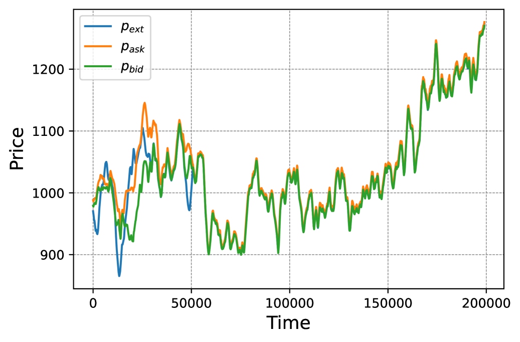
(a) $p_{ask}$, $p_{bid}$ and $p_{ext}$

(b) Mid price deviation

(c) Spread

Figure 1. The conjectured reward for the model-free algorithm trains the agent to track the external hidden price, eventually approaching the performance of the optimal Bayesian algorithm. Figure reference in Section 5.6.

Sudden price jumps. Secondly, we observed what happens when there is a sudden jump in the external market price. In that case as well, as shown in Figure [2], the algorithm tracks the external price correctly.

(a) $p_{ask}$, $p_{bid}$ and $p_{ext}$

(b) Mid price deviation

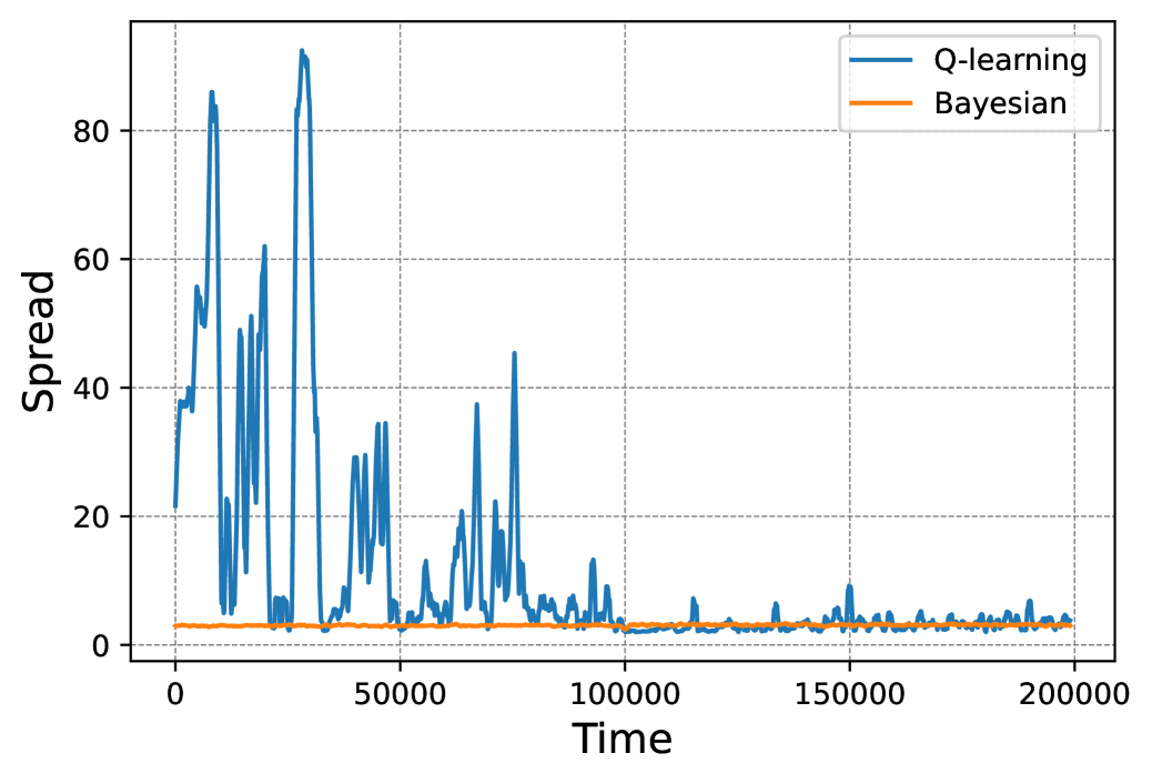
(c) Spread

Figure 2. The conjectured reward for the model-free algorithm trains the agent to track the external hidden price, even in the presence of large price jumps. Figure reference in Section 5.6.

Changing market conditions. Thirdly, we check the robustness of the algorithm to changing market conditions. This is the key to verifying its model-free nature. To do that, we vary the trader informedness $\alpha$ and underlying price volatility $\sigma$ with time by making them follow a driftless random walk in the range $[0,1]$. We find that the algorithm obtains near zero spread and mid-price deviation in this situation as well, as shown in Figure [3].

(a) Erratic changes in the external market conditions : trader informedness and price volatility

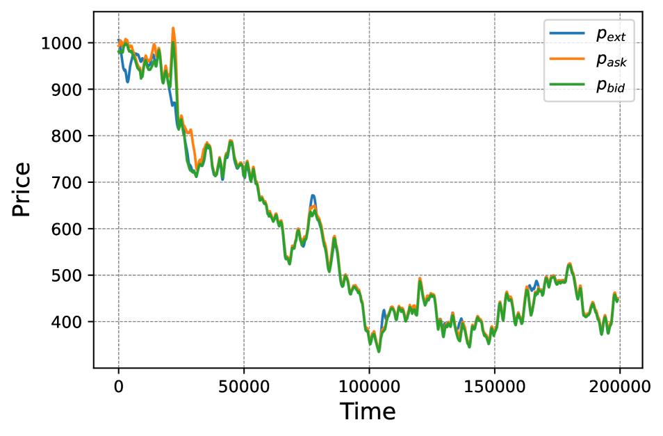
(b) Ask and Bid recommended by the data-driven algorithm track the hidden external price

Figure 3. Even in the presence of erratic changes in the market conditions (Figure (a)), our data-driven algorithm for market making tracks the external hidden price with no prior training (Figure(b))

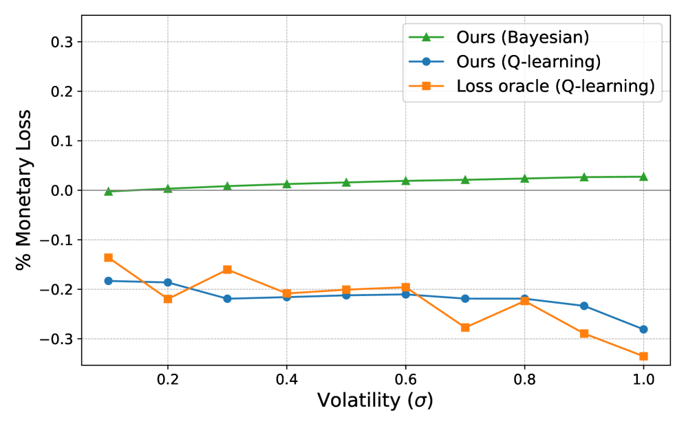
(a) Percentage monetary loss per trade of our market maker is comparable with the algorithm which has access to the loss oracle

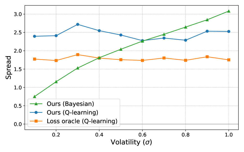
(b) Larger spread observed without access to the loss oracle

Figure 4. Algorithm 2 gives us comparable monetary loss per trade as running the algorithm with an oracle. The Bayesian algorithm 1 gives loss close to zero, which is optimally efficient. All plots are averaged over values of informedness $\alpha$.

Comparing monetary loss: We compared the percentage monetary loss per trade for each of our market makers, with the algorithm in (chan2001, ). This work also uses Q-learning, but for a reward that has direct access to the hidden external price $p_{ext}$ and hence acts like a loss oracle. The reward function in (chan2001, ), is of the form $r_{t}=-l_{t}-\mu(p_{a}^{t}-p_{b}^{t})^{2}$, where $l_{t}$ is the monetary loss as defined in (4). In our case, despite no access to such a loss oracle, we find that the average monetary loss per trade (around $0.2\%$) is comparable with that of (chan2001, ) for all values of volatility $\sigma$ (Figure [4(a)]). As expected, the Bayesian algorithm 1 is better than either of the others, giving us the optimally efficient zero loss. We also observe that, due to access to less information about $p_{ext}$ than (chan2001, ), algorithm 2 has to resort to a larger spread (Figure [4(b)]).

We compared the loss performance of our algorithms with the alternative approach (Section 5.1) of using stochastic variational inference to estimate trader informedness and volatility first, and then using those estimates in our Bayesian approach. We got a consistently high loss (around 2%) , which is at least $10$ times the loss we got by other approaches. Additionally, the running time of this algorithm took on an average $40-50$ times that of any other algorithms to compute the ask and bid prices in each iteration.

5.7. General trader behavior

The model of trader behavior as outlined in Section 3 is restrictive, in the sense that real traders lie on a spectrum of “informedness” about the external price, instead of being purely informed or uninformed. To remedy this, we modify the environment to have traders that see a noisy version of the hidden price. That is, every trader sees an observation $p_{trader}^{t}=p_{ext}^{t}+\eta_{t}$ where $\eta_{t}$ is i.i.d noise (note that the model in Section 3 is just a special case of this). Then, the trader buys if $p_{trader}^{t}>p_{a}^{t}$, sells if $p_{trader}^{t}<p_{b}^{t}$ and does neither otherwise. We experimented with three types of noise - additive Gaussian, additive Laplace, and log-Normal.

Because the model to be estimated becomes more complex, we replace the $Q-$table with a neural network (mnih2013playing, ). The neural network takes the trade history $(d_{t-H},\cdots,d_{t})$ as a vector input instead of treating the sum ($n_{t}=\sum_{\tau=t-H}^{t}d_{\tau}$) of the trade history as a scalar input. Using this approach , we found that the market maker could handle even more sophisticated forms of trader behavior (Figure [5]).

We observe that the algorithm trained on any one form of them is robust to a change in underlying trader distribution. In particular, Figure [5(a)] shows the ask and bid prices for an optimal Bayesian trader as per Algorithm 1. We then train the DQN on traders with Gaussian noise, which reach spread and mid-price deviation values similar to the Bayesian case, as shown in Figure [5(b)]. We observe that the same agent then effectively tracks the external price when the types of noise that traders see is changed to Laplace and log-Normal in Figure [5(c)] and Figure [5(d)] respectively.

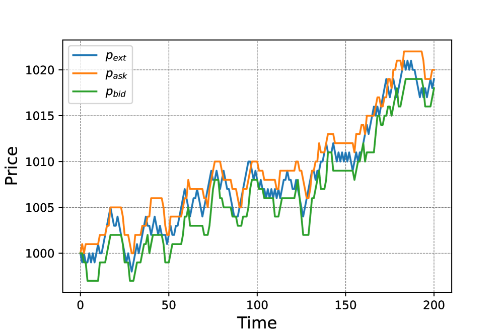
(a) Using the optimal Bayesian algorithm to track external price - with known underlying model parameters

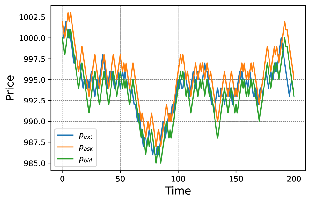
(b) Trader observes external price through Gaussian noise. Market Maker based on a DQN is trained on this trader behavior - tracking is achieved with similar average spread and loss as the Bayesian model

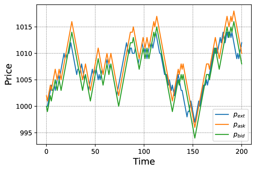
(c) Trader observes external price through Laplace noise. Market maker tracks price effectively without any prior training on this noise model.

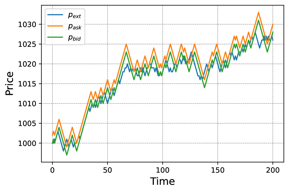
(d) Trader observes external price through log-normal noise. Market maker tracks price effectively without any prior training on this noise model.

Figure 5. Algorithm 2 is robust to changes in underlying trader behavior.

6. System design for an on-chain implementation

We propose that the data-driven market maker described in Algorithm 2 can be implemented in a manner similar to an optimistic rollup scheme (optimisticRollupsEthereum, ). We now give details of the implementation, and refer to Figure [6] for an overview.

Smart contract: The main part of this implementation is the $ZeroSwap$ smart contract, which would store the latest version of the Q-table used to execute trades. The blockchain that the contract resides on can be a Layer 1 such as Ethereum, or a Layer 2 rollup, such as Arbitrum (arbitrum, ) or Optimism (optimism, ). The contract performs trade execution based on solutions posted, and also resolves any challenges to those solutions. We explain these terms in what follows.

Agents: The smart contract interacts with three types of agents: traders, validators and challengers. Traders wish to have their trades executed by the protocol. Validators put up stake in the protocol (i.e. lock up a specific token in the smart contract), and in return, get selected to run Algorithm 2 off-chain and post solutions. The stake also acts as a security deposit to deter validators from misbehaving. Challengers ensure the security of the protocol by verifying the validity of the posted solutions and post challenges if they can find better solutions.

Trading protocol: Firstly, traders post trade requests as part of a block of transactions on the blockchain. These indicate their intent to buy or sell the asset from the market maker. Next, the validators collect all trade requests in a block. A chosen validator, called a proposer, then runs one iteration of Algorithm 2 for each trade, and posts the solution on the next block. This solution comprises of the prices at which the trades are to be executed, and an update to the on-chain Q-table. The protocol smart contract would receive this solution from a valid proposer, and execute the trades optimistically along with updating the on-chain Q-table according to the solution. We see that, in this blockchain implementation, the trades are processed in batches (corresponding to blocks). This implies that only the external price jump that happens from one block to the next matters. Thus, we have a situation where a price jump has happened, and that jump is to be inferred from a given batch of trades that was collected in a block. We know that this can be done with exponentially vanishing error (in the number of trades) as shown in Corollary 5.2.

Challenge protocol: The execution of trades outlined above is made secure by the presence of challengers. A challenger can post a challenge on-chain to be processed by the smart contract. The challenge consists of a reference to a trade request the challenger thinks was executed incorrectly, and an alternate solution pointing to the $(n_{t},a)$ pair (see line (12) of Algorithm 2) that corresponds to an entry of the Q-table providing a better solution. The smart contract verifies in just one step whether this challenge is valid by querying the lookup table and comparing the values, thus checking if the $\arg\max$ operation was executed correctly by the proposer. A fault in the Q-table update on line (21) can be challenged in a similar manner. In this case as well, the challenger only posts an alternate solution (an $(n_{t},a)$ pair) to the $\max$ operation used in the update, and the smart contract verifies its validity by looking it up in the Q-table.

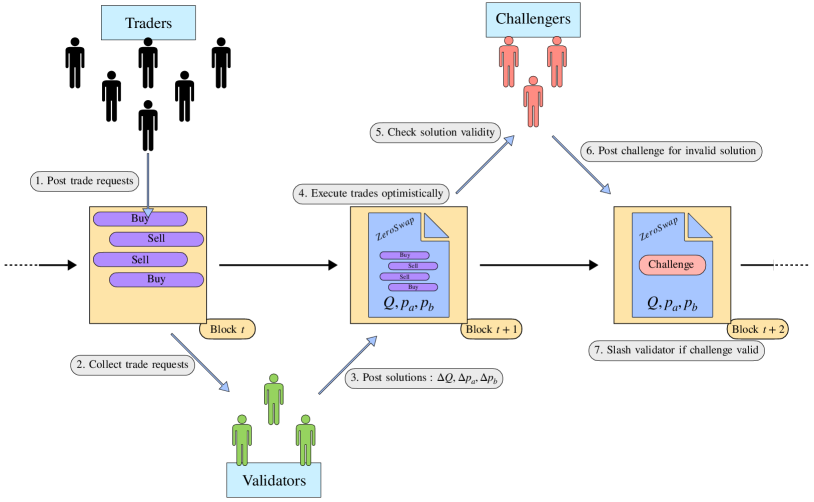
Figure 6. Design for an on-chain implementation of ZeroSwap.

Computational costs: In the smart contract, the main state variable to be tracked is the $Q-$table, which is of the size $|{O}|\times|{A}|$. In our case, the cardinality of the observation space $O$ equals the difference between the maximum and minimum trade imbalance, which is $2H$. The action space $A$ is just $\{-1,0,+1\}\times\{-1,0,+1\}$. Thus, the direct implementation of the RL model would involve tracking and updating a table with $18H$ entries. Even for a trade history size $H=100$, the $Q-$table size ($1800$) is much smaller than the liquidity vector tracked in AMMs such as Uniswap-v3 (uniswapv3, ) for a single pool (which is of size $170,000$). Processing a single trade in Q-learning involves only modifying a single entry of the Q-table with a convex combination operation. This incurs similar computational cost as the simple addition operations required to update the liquidity vector after a trade in Uniswap-v3. Doing the $\arg\max$ operation off-chain lowers the gas usage of Q-learning considerably, since only algebraic operations remain to be done on-chain. However, note that these calculations are for only a toy model with fixed trade size and no inventory constraints.

Incentives: In the case that an invalid execution is detected by the smart contract through the challenges posted, the proposer whose solution was challenged would get their stake slashed. The staking infrastructure and the slashing conditions can be enforced using restaking services such as Eigenlayer (eigenlayer, ). This allows the validators to stake the native token of the underlying blockchain without the need to create $ZeroSwap$-specific tokens for managing incentives.

Potential MEV: There is a strong incentive for the miners of the underlying blockchain to to extract MEV (daian2019flash, ) from $ZeroSwap$. Because the Q-table and corresponding algorithm are public, the miner can calculate the optimal trade requests to frontrun and hence make a profit from other trades. This can be avoided by adding a batching operation that the validator of $ZeroSwap$ must perform before running the iteration of the Q-learning algorithm. A simple solution is to match buy and sell trades first, and then satisfy the surplus (which would be a single large buy trade or sell trade) as per the ask/bid recommendations of the algorithm (cowswap, ; ramseyer2023augmenting, ).

7. Discussion

Exploiting information present in trades for efficiency. In Section 5, we observed that a model-free algorithm can be obtained to solve optimal market making by looking just at the incoming trades, and provided theoretical guarantees on its performance. The static curves used in AMMs today do not take into account recent past history of trades, while we propose to have dynamically adjusting ask and bid prices to make use of the information available to us through those trades as much as possible.

Generalizing to variable trade size. The model-free algorithm specified in this work does not take into account variable trade size, since we assume that the liquidity of the market maker are deep enough so that a single trade does not have a significant price impact. Our ongoing work involves deriving an algorithm for that case by using a dynamic CFMM bonding curve (instead of dynamic ask and bid prices), which is parameterized. This deals with the case of moderate volume and liquidity markets. An adaptive algorithm is then used to control the curve parameters, so as to satisfy the conditions analogous to (2) and (3) for optimal market making. Just as in the case outlined in the current work, we find that using the information at hand in the form of incoming trades decreases the monetary loss that the market makers face. This on-going work is the topic of a companion paper.

Inventory considerations. Our algorithms do not take into account constraints on the inventory of the market maker. The inventory preference of the LPs can be encoded as utility functions, which can be mapped to a family of bonding curves (goyal2023finding, ; frongillo2023axiomatic, ). Our method can help decide which particular curve in that family should be used to offer the most efficient price given trading history.

Adding data-driven adaptivity to DeFi. This work further makes a case for data-driven adaptive algorithms for DeFi in general. Future work would include bringing algorithms from reinforcement learning and stochastic control to applications such as lending protocols, treasury management and tokenomic monetary policy.

Appendix A Theoretical guarantees

In this section, we provide proofs for the following results

1. Bounds on the performance of the Bayesian algorithm

2. Bounds on the performance of the data-driven algorithm with the conjectured reward function

A.1. Proof of Theorem 4.1 for a special case

At time $t=0$, assume that the external price jumps up to $p_{u}$ with probability $1-\sigma$ and jumps to $p_{l}$ with probability $\sigma$. After this, assume that the market maker follow the Glosten-Milgrom policy using the Bayes’ rule.

At time $t$, we have a trading history $\langle d_{i}\rangle_{i=1}^{t}$ along with a history of prices $\langle(p_{a}^{i},p_{b}^{i})\rangle_{i=1}^{t}$. Define $q_{i}=Pr[d_{i}=+1|p_{a}^{i},p_{b}^{i},p_{ext}=p_{l}]$ and $r_{i}=Pr[d_{i}=+1|p_{a}^{i},p_{b}^{i},p_{ext}=p_{u}]$. Note that, given the external price and the sequence of ask and bid prices, the trades $d_{i}$ are independent, with their probabilities being completely determined by the GM model in terms of $\alpha$ and $\sigma$. Thus, given a sequence of trades, we have

(13) $$Pr[\langle d_{i}\rangle_{i=1}^{t}|p_{ext}=p_{l},]=\prod_{i:d_{i}=1}q_{i}\prod_{i:d_{i}=-1}(1-q_{i}).$$

This gives, using Bayes’ rule

(14) $$Pr[p_{ext}=p_{l}|\mathcal{H}_{t}]=\frac{\sigma\prod_{i:d_{i}=1}q_{i}\prod_{i:d_{i}=-1}(1-q_{i})}{\sigma\prod_{i:d_{i}=1}q_{i}\prod_{i:d_{i}=-1}(1-q_{i})+(1-\sigma)\prod_{i:d_{i}=1}r_{i}\prod_{i:d_{i}=-1}(1-r_{i})},$$

where $\mathcal{H}_{t}$ consists of the history $\langle d_{i}\rangle_{i=1}^{t},\langle(p_{a}^{i},p_{b}^{i})\rangle_{i=1}^{t}$.

The above equation tells us the market maker’s posterior belief about the external price at time $t$, given the history of trades and prices. Now consider the log-likelihood ratio

(15) $$\log\left(\frac{Pr[p_{ext}=p_{l}|\mathcal{H}_{t}]}{Pr[p_{ext}=p_{u}|\mathcal{H}_{t}]}\right) =\log\left(\frac{\sigma\prod_{i:d_{i}=1}q_{i}\prod_{i:d_{i}=-1}(1-q_{i})}{(1-\sigma)\prod_{i:d_{i}=1}r_{i}\prod_{i:d_{i}=-1}(1-r_{i})}\right).$$

We know that $p_{l}\leq E[p_{ext}|\mathcal{H}_{t}]\leq p_{u}$, which implies that the GM policy always recommends bid and ask prices between $p_{l}$ and $p_{u}$. This simplifies things further, since now we have $q_{i}=\frac{1-\alpha}{2}:=q$ and $r_{i}=\frac{1+\alpha}{2}:=r$. This gives us

(16) $$\log\left(\frac{Pr[p_{ext}=p_{l}|\mathcal{H}_{t}]}{Pr[p_{ext}=p_{u}|\mathcal{H}_{t}]}\right) =\log\left(\frac{\sigma q^{b}(1-q)^{s}}{(1-\sigma)r^{b}(1-r)^{s}}\right)$$

(17) $$=\log\frac{\sigma}{1-\sigma}+b\log\frac{q}{r}+s\log\frac{1-q}{1-r},$$

where $b$ and $s$ are the number of buy and sell trades respectively.

Dividing both sides by the total number of trades $b+s$ and taking the limit as $b+s\rightarrow\infty$, we get that, as $b+s\rightarrow\infty$,

(18) $$\frac{1}{b+s}\log\left(\frac{Pr[p_{ext}=p_{l}|\mathcal{H}_{t}]}{Pr[p_{ext}=p_{u}|\mathcal{H}_{t}]}\right) \longrightarrow D_{\mathrm{KL}}(\mathbf{q}||\mathbf{r})\ \ \ \mathrm{if\ }p_{ext}=p_{l}$$

(19) $$\longrightarrow-D_{\mathrm{KL}}(\mathbf{r}||\mathbf{q})\ \ \ \mathrm{if\ }p_{ext}=p_{u},$$

where $\mathbf{q}=[\frac{1-\alpha}{2},\frac{1+\alpha}{2}],\mathbf{r}=[\frac{1+\alpha}{2},\frac{1-\alpha}{2}]$. Thus, for a non-trivial number of informed traders ($\alpha>0$), the KL-divergence would be always strictly positive. This implies that the posterior $(Pr[p_{ext}=p_{l}|\mathcal{H}_{t}],Pr[p_{ext}=p_{u}|\mathcal{H}_{t}])$ converges to either $(1,0)$ or $(0,1)$ depending on whether $p_{ext}$ is $p_{l}$ or $p_{u}$ respectively. This proves that both bid and ask converge to the right price as well. The only case where the convergence does not happen is when the KL divergence is exactly zero, which happens when $\alpha=0$ (no informed traders).

Suppose the actual price is $p_{l}$. Then, the explicit bid and ask at each time $t$ evolves as

(20) $$p_{a} =\frac{p_{l}\sigma q^{b+1}(1-q)^{s}+p_{u}(1-\sigma)r^{b+1}(1-r)^{s}}{\sigma q^{b+1}(1-q)^{s}+(1-\sigma)r^{b+1}(1-r)^{s}}$$

(21) $$\rightarrow\frac{(1-\alpha)p_{l}+(1+\alpha)p_{u}e^{-D_{\mathrm{KL}}(\mathbf{q}||\mathbf{r})t}}{(1-\alpha)+(1+\alpha)e^{-\mathrm{KL}(\mathbf{q}||\mathbf{r})t}}.$$

Similarly, the bid price evolves as

(22) $$p_{b}\rightarrow\frac{(1+\alpha)p_{l}+(1-\alpha)p_{u}e^{-D_{\mathrm{KL}}(\mathbf{q}||\mathbf{r})t}}{(1+\alpha)+(1-\alpha)e^{-\mathrm{KL}(\mathbf{q}||\mathbf{r})t}},$$

where we see that both ask $p_{a}$ and bid $p_{b}$ converge exponentially to the actual price $p_{l}$. We further observe that the rate of exponential convergence is increases with the informedness of the trader distribution, approaching infinity as $\alpha\rightarrow 1$.

A.2. Proof of Theorem 4.1 for the general case

For a general single jump, we use propositions from [27] as guidance to prove that the ask and bid converge to the true price. Assume that the true price jumps to $p_{ext}^{*}$, with the p.d.f. of the jump being known to the market maker as $f(p_{ext})$. We denote the ask and bid price recommendations of the Bayesian algorithm by $p_{a}^{t},p_{b}^{t}$ respectively.

The first lemma we prove guarantees convergence of the spread.

Lemma A.1.

If we define $\bar{S}_{T}=\frac{1}{T}\sum_{t=0}^{T}E[(p_{a}^{t}-p_{b}^{t})^{2}]$, then for $\alpha<1$, we get

(23) $$\bar{S}_{T}\leq\frac{8\mathrm{var}(p_{ext})}{(1-\alpha)^{2}T}.$$

Proof.

First, we prove that the spread goes to zero. The key idea used here is the fact that the variance of a random variable decreases on conditioning.

Define $p_{t}=E[p_{ext}|\mathcal{H}_{t}]$. Note that $p_{t}$ is a martingale w.r.t. $\mathcal{H}_{t}$, since $E[p_{t}|H_{t-1}]=p_{t-1}$. Thus, we have

(24) $$\mathrm{var}(p_{ext}) \geq\mathrm{var}(p_{t})$$

(25) $$=\mathrm{var}\left(\sum_{t=0}^{T}(p_{t}-p_{t-1})\right)\ \ \ \ \ \mathrm{where}\ p_{0}=E[p_{ext}],\ p_{-1}=0$$

(26) $$=\sum_{t=0}^{T}E[(p_{t}-p_{t-1})^{2}]+\sum_{t=0}^{T}\sum_{k<t}E[(p_{t}-p_{t-1})(p_{k}-p_{k-1})]$$

(27) $$=\sum_{t=0}^{T}E[(p_{t}-p_{t-1})^{2}],$$

since $E[(p_{t}-p_{t-1})(p_{k}-p_{k-1})]=E[E[(p_{t}-p_{t-1})(p_{k}-p_{k-1})|\mathcal{H}_{t-1}]]=E[(p_{k}-p_{k-1})E[(p_{t}-p_{t-1})|\mathcal{H}_{t-1}]]=0$ by the martingale property.

Now, note that

(28) $$(p_{a}^{t}-p_{b}^{t})^{2} \leq 2(p_{a}^{t}-p_{t-1})^{2}+2(p_{b}^{t}-p_{t-1})^{2}$$

(29) $$\leq\frac{2(p_{a}^{t}-p_{t-1})^{2}}{Pr[d_{t}=-1|\mathcal{H}_{t-1}]}+\frac{2(p_{b}^{t}-p_{t-1})^{2}}{Pr[d_{t}=+1|\mathcal{H}_{t-1}]}$$

(30) $$=\frac{2(p_{a}^{t}-p_{t-1})^{2}Pr[d_{t}=+1|\mathcal{H}_{t-1}]+2(p_{b}^{t}-p_{t-1})^{2}Pr[d_{t}=-1|\mathcal{H}_{t-1}]}{Pr[d_{t}=-1|\mathcal{H}_{t-1}]Pr[d_{t}=+1|\mathcal{H}_{t-1}]}$$

(31) $$\leq 2\frac{E[(p_{t}-p_{t-1})^{2}|\mathcal{H}_{t-1}]}{\left(\frac{1-\alpha}{2}\right)^{2}}.$$

(32) $$\implies E[(p_{a}^{t}-p_{b}^{t})^{2}] \leq\frac{8E[(p_{t}-p_{t-1})^{2}]}{(1-\alpha)^{2}}.$$

(33) $$\implies\frac{1}{T}\sum_{t=0}^{T}E[(p_{a}^{t}-p_{b}^{t})^{2}] \leq\frac{8\mathrm{var}(p_{ext})}{(1-\alpha)^{2}T}.$$

∎

Next, we show that the ask and bid indeed converge to the true external price.

Lemma A.2.

If $p_{ext}^{*}$ denotes the value that the external price $p_{ext}$ jumps to, then we have

(34) $$Pr[|p_{ext}^{*}-p_{a}^{t}|\geq\epsilon] \rightarrow 0$$

(35) $$Pr[|p_{ext}^{*}-p_{b}^{t}|\geq\epsilon] \rightarrow 0,$$

as $t\rightarrow\infty$. This shows that the Bayesian policy converges to the true price eventually.

Proof.

We have that

(36) $$p_{a}^{t} =E[p_{ext}|\mathcal{H}_{t-1},d_{t}=+1]$$

(37) $$=\alpha E[p_{ext}|\mathcal{H}_{t-1},p_{ext}>p_{a}^{t}]+(1-\alpha)p_{t-1}$$

(38) $$\geq\alpha E[p_{ext}|\mathcal{H}_{t-1},p_{ext}>p_{t-1}]+(1-\alpha)p_{t-1}.$$

(39) $$\implies p_{a}^{t}-p_{t-1} \geq\alpha E[p_{ext}-p_{t-1}|\mathcal{H}_{t-1},p_{ext}>p_{t-1}]$$

(40) $$\geq\alpha\epsilon Pr[p_{ext}-p_{t-1}\geq\epsilon|\mathcal{H}_{t-1},p_{ext}>p_{t-1}]$$

(41) $$\geq\alpha\epsilon Pr[p_{ext}-p_{t-1}\geq\epsilon|\mathcal{H}_{t-1}].$$

We know that since $p_{a}^{t}\geq p_{t-1}\geq p_{b}^{t}$ and the spread goes to zero, we have $p_{a}^{t}-p_{t-1}\rightarrow 0$. Thus, for any $\epsilon>0$, we get $Pr[p_{ext}-p_{t-1}\geq\epsilon|\mathcal{H}_{t-1}]\rightarrow 0$. Similarly, we get $Pr[p_{ext}-p_{t-1}\leq-\epsilon|\mathcal{H}_{t-1}]\rightarrow 0$.

∎

For proving the exponential rate of decay in spread, we use equation (94), which shall be proven in later sections, under the assumption that $\frac{p_{a}^{2}}{\mathrm{var}(p)}\geq\epsilon>0$ at any time. This is a valid assumption since the $E[p_{a}]$ is assumed to be equal to $0$ while deriving (94). Thus, conditioning on a buy trade would only increase the ask price. Therefore, we have that $p_{a}=E[p_{a}|d_{t}=+1]>0$.

Rewriting (94) by replacing the total variance $K_{0}+\sigma T$ with $\mathrm{var}(p_{T})$ gives us

(42) $$\mathrm{var}(p_{T+1}) \leq\mathrm{var}(p_{T})\left(1-\alpha/2\left(1-\sqrt{1-\frac{1-\alpha}{\alpha}\epsilon}\right)^{2}\right).$$

Since there are no price jumps and only trades in the time steps before $T+1$, this implies that

(43) $$\mathrm{var}(p_{T+1}) \leq\mathrm{var}(p_{1})\left(1-\alpha/2\left(1-\sqrt{1-\frac{1-\alpha}{\alpha}\epsilon}\right)^{2}\right)^{T},$$

which confirms that the variance of the belief goes down exponentially with time. Since the expected squared spread $p_{a}^{2}$ is upper bounded by the variance, we have that the spread also decays exponentially with time.

A.3. Proof of Theorem 4.2

When the price $p_{ext}$ follows a random walk, we observe empirically that the GM ask and bid prices manage to track $p_{ext}$ closely, but always with a non-zero spread. What we now prove is that the spread does not diverge, given that the traders bring in some useful information. We introduce a constant trader arrival rate $\lambda$, i.e. a trader arrives every $1/\lambda$ time steps.

Let $p_{a}^{T}-p_{b}^{T}=\mathcal{O}(g(T|\sigma,\alpha,\lambda))$.

In this case, we want to answer the following three questions :

1. What is $g$ when $\lambda=0$? (Empirically this is $\mathcal{O}(\sqrt{T})$)

2. What is $g$ when $\lambda>0$? (Empirically this is $\mathcal{O}(1)$ even for a small $\lambda$)

3. What is $g$ when $\lambda\gg\sigma$? ($=\mathcal{O}(e^{-kT})$ from Section A.1)

In this section, we prove that in the absence of trades, the spread diverges at a rate of $\sqrt{T}$. Furthermore, we formalize the intuition that even sparse trading activity narrows down the support of the belief and keeps the spread from diverging.

A.3.1. Spread behavior in the absence of trades

We derive the spread divergence rate in case of an external price following a simple random walk with jump probability $\sigma$ and no trades taking place. We denote the belief over external price at time $t$ by $f_{t}(.)$

Lemma A.3.

In the absence of any trades, the variance of the Bayesian belief $f_{t}(.)$ over the external price obeys the following rule

(44) $$\mathrm{var}(f_{t})=\mathrm{var}(f_{t-1})+\sigma$$

Proof.

(45) $$\mathrm{var}(f_{t}) =\sum_{p}p^{2}f_{t}(p)$$

(46) $$=\sum_{p}p^{2}((1-\sigma)f_{t-1}(p)+\sigma/2f_{t-1}(p-1)++\sigma/2f_{t-1}(p+1))$$

(47) $$=(1-\sigma)\sum_{p}p^{2}f_{t-1}(p)+\sigma/2\sum_{p}(p-1+1)^{2}f_{t-1}(p-1)+\sigma/2\sum_{p}(p+1-1)^{2}f_{t-1}(p+1)$$

(48) $$=\left[(1-\sigma)\sum_{p}p^{2}f_{t-1}(p)+\sigma/2\sum_{p}(p-1)^{2}f_{t-1}(p-1)+\sigma/2\sum_{p}(p+1)^{2}f_{t-1}(p+1)\right]$$

(49) $$+\left[\sigma/2\sum_{p}f_{t-1}(p-1)+\sigma/2\sum_{p}f_{t-1}(p+1)\right]$$

(50) $$+\left[\sigma/2\sum_{p}(p-1)f_{t-1}(p-1)+\sigma/2\sum_{p}(p+1)f_{t-1}(p+1)\right]$$

(51) $$=\left[\mathrm{var}(f_{t})\right]+\left[\sigma\right]+\left[0\right].$$

∎

We now derive an upper bound on the ask price.

(52) $$E_{t}^{2}[p|d_{t}=+1] \leq E_{t}[p^{2}|d_{t}=+1]$$

(53) $$=\sum_{p}f_{t}(p|d_{t}=+1)p^{2}$$

(54) $$=\sum_{p}\frac{(1-\alpha)+2\alpha\mathbf{1}_{p\geq p_{a}^{t}}}{(1-\alpha)+2\alpha Pr[p\geq p_{a}]}f_{t}(p)p^{2}$$

(55) $$\leq\sum_{p}\frac{1+\alpha}{1-\alpha}f_{t}(p)p^{2}$$

(56) $$=\frac{1+\alpha}{1-\alpha}\sigma t.$$

(57) $$\implies p_{a}^{t} \leq\sqrt{\frac{1+\alpha}{1-\alpha}\sigma t}.$$

Note that the above argument is valid when $1-\alpha>0$. For $\alpha=1$, we get $p_{a}^{t}=t$.

We can get the following tighter upper bound than the above by using the definition of the ask price.

Lemma A.4.

Assume that the expected initial price $E[p_{ext}^{0}]=0$. Then, the ask price of the Bayesian market maker is upper bounded as

(58) $$p_{a}^{t} \leq\sqrt{\frac{\alpha}{2(1-\alpha)}\sigma t}.$$

Proof.

We know that

(59) $$p_{a}^{t} =E[p|d_{t}=+1].$$

Using the Bayes rule, and that $E[p_{ext}^{0}]=0$, we can write the RHS as

(60) $$p_{a}^{t} =\frac{2\alpha}{1-\alpha+2\alpha Pr[p\geq p_{a}^{t}]}\sum_{p}\mathbf{1}_{\{p\geq p_{a}^{t}\}}pf_{t}(p)$$

(61) $$\leq\frac{2\alpha}{1-\alpha+2\alpha Pr[p\geq p_{a}^{t}]}(\sum_{p}\mathbf{1}_{\{p\geq p_{a}^{t}\}}f_{t}(p))^{1/2}(\sum_{p}p^{2}f_{t}(p))^{1/2}$$

(62) $$=\frac{2\alpha}{1-\alpha+2\alpha Pr[p\geq p_{a}^{t}]}(Pr[p\geq p_{a}^{t}])^{1/2}(\sigma t)^{1/2}.$$

(63) $$\implies(1-\alpha +2\alpha Pr[p\geq p_{a}^{t}])p_{a}^{t}\leq 2\alpha\sqrt{\sigma t}\sqrt{Pr[p\geq p_{a}^{t}]}.$$

(64) $$\implies(2\alpha p_{a}^{t}) Pr[p\geq p_{a}^{t}]-2\alpha\sqrt{\sigma t}\sqrt{Pr[p\geq p_{a}^{t}]}+p_{a}^{t}(1-\alpha)\leq 0.$$

The roots of the quadratic expression (in $\sqrt{Pr[p\geq p_{a}]}$) on the LHS of (64) are

(65) $$\left\{\frac{\sqrt{\sigma t}}{2p_{a}^{t}}-\sqrt{\frac{\sigma t}{4(p_{a}^{t})^{2}}-\frac{1-\alpha}{2\alpha}},\frac{\sqrt{\sigma T}}{2p_{a}^{t}}+\sqrt{\frac{\sigma t}{4(p_{a}^{t})^{2}}-\frac{1-\alpha}{2\alpha}}\right\}$$

Because the quadratic expression has a positive coefficient of the squared term, these roots must be real for the expression to ever be negative. This gives us the result.

∎

From the above proof, we notice that the following must also hold for the quadratic expression in (64) to be $\leq 0$. We shall use this inequality in the subsequent section. In fact, we see from the above proof that we have the following lemma

Lemma A.5.

If the initial belief of the market maker over the external market price is such that $E[p_{ext}^{0}]=0$, then in the absence of trades, we have

(66) $$\frac{\sqrt{\mathrm{var}(p_{ext}^{T})}}{2p_{a}}-\sqrt{\frac{\mathrm{var}(p_{ext}^{T})}{4p_{a}^{2}}-\frac{1-\alpha}{2\alpha}}\leq\sqrt{Pr[p\geq p_{a}^{T}]}\leq\frac{\sqrt{\mathrm{var}(p_{ext}^{T})}}{2p_{a}}+\sqrt{\frac{\mathrm{var}(p_{ext}^{T})}{4p_{a}^{2}}-\frac{1-\alpha}{2\alpha}},$$

where $\mathrm{var}(p_{ext}^{T})$ is the variance of the market maker’s belief at time $T$.

We now show a lower bound on the ask price, which completes the proof on the rate of growth of the spread in absence of trades.

Lemma A.6.

Assuming that the expected initial price $E[p_{ext}^{0}]$ is zero for simplicity. The ask price of the Bayesian market maker is lower bounded as

(67) $$p_{a}^{t} \geq\frac{\alpha}{1+2\alpha}\sqrt{\frac{2\sigma t}{\pi}}$$

Proof.

(68) $$p_{a}^{t} =\frac{2\alpha}{1-\alpha+2\alpha Pr[p\geq p_{a}^{t}]}\sum_{p}\mathbf{1}_{\{p\geq p_{a}\}}pf_{t}(p).$$

(69) $$\implies p_{a}^{t} \geq\frac{2\alpha}{1+\alpha}\sum_{p=p_{a}^{t}}^{T}pf_{t}(p)$$

(70) $$=\frac{2\alpha}{1+\alpha}\left(\sum_{p=0}^{T}pf_{t}(p)-\sum_{p=0}^{p_{a}^{t}}pf_{t}(p)\right)$$

(71) $$=\frac{2\alpha}{1+\alpha}\left(\frac{E[|p|]}{2}-\sum_{k=1}^{p_{a}^{t}}Pr[p_{a}^{t}\geq p\geq k]\right)$$

(72) $$\geq\frac{2\alpha}{1+\alpha}\left(\frac{E[|p|]}{2}-\sum_{k=1}^{p_{a}^{t}}Pr[p\geq k]\right)$$

(73) $$\geq\frac{2\alpha}{1+\alpha}\left(\frac{E[|p|]}{2}-\frac{p_{a}^{t}}{2}\right).$$

(74) $$\implies p_{a}^{t} \geq\frac{\alpha}{1+2\alpha}E[|p|].$$

(75) $$\implies p_{a}^{t} \geq\frac{\alpha}{1+2\alpha}\sqrt{\frac{2\sigma t}{\pi}},$$

where we have used the formula for the expected absolute deviation for a simple random walk [11]. ∎

Thus, the ask price is upper and lower bounded by terms that grow with $\sqrt{\sigma t}$, which proves the first part of the theorem.

A.3.2. Spread behavior in the presence of trades

In the previous section, we proved that the spread diverges exactly at a rate of $\sqrt{T}$ when $\alpha<1$ and at the rate of $T$ when $\alpha=1$, in the absence of trades. In this section, we derive results on spread behavior in presence of trades. Empirically, we see that even for very sparse trading, the spread does not diverge (is $\mathcal{O}(1)$).

First, let us calculate the variance of the belief after $T+1$ time steps, where $T=1/\lambda$. That is, we have $T$ time steps where no trades occur and the $T+1^{th}$ time step where a single trade occurs. Let the ask, bid and external prices just before the trade be $p_{a},p_{b},p_{ext}$ respectively. We drop the $T$ superscript for simplicity. Also, assume that the variance of the initial belief distribution is $K_{0}$, and that the mean of the belief is $0$ for simplicity. What we aim to prove is that, if the $K_{0}$ is large enough, then the variance of the belief just after the trade at $T+1$ steps is less than $K_{0}$. Let the trade that happens at $T+1$ be denoted by $d$.

Then, the expected variance of the belief just after the last time step (when the trade happens) is given by

(76) $$E[E[(p_{ext}-E[p_{ext}|d])^{2}|d]] =E[(p_{ext}-E[p_{ext}|d])^{2}].$$

Now, we write this variance as the difference between two terms, as shown in the following lemma.

Lemma A.7.

The expected variance of the belief just after a trade can be written as

(77) $$E[(p_{ext}-E[p_{ext}|d])^{2}] =E[(p_{ext}-E[p_{ext}])^{2}]-E[(E[p_{ext}|d]-E[p_{ext}])^{2}].$$

Proof.

We first start with the expression for the variance just before the trade, and then write it as the sum of the variance just after the trade and another non-negative term.

(78) $$E[(p_{ext}-E[p_{ext}])^{2}] =E[(p_{ext}-E[p_{ext}|d]+E[p_{ext}|d]-E[p_{ext}])^{2}]$$

(79) $$=E[(p_{ext}-E[p_{ext}|d])^{2}+E[(E[p_{ext}|d]-E[p_{ext}])^{2}]$$

(80) $$+2E[(p_{ext}-E[p_{ext}|d])(E[p_{ext}|d]-E[p_{ext}])]$$

(81) $$=E[(p_{ext}-E[p_{ext}|d])^{2}+E[(E[p_{ext}|d]-E[p_{ext}])^{2}]$$

(82) $$+2E[\ p_{ext}E[p_{ext}|d]+E[p_{ext}|d]E[p_{ext}]-E^{2}[p_{ext}|d]-p_{ext}E[p_{ext}]\ ].$$

The last term in the above equation can be written as

(83) $$E[p_{ext}E[p_{ext}|d]]+E[E[p_{ext}|d]E[p_{ext}]]-E[E^{2}[p_{ext}|d]]-E[p_{ext}E[p_{ext}]].$$

Observe that using $E[E[p_{ext}|d]]=E[p_{ext}]$, the second and fourth terms cancel out. We now group the first and third terms together, which gives us

(84) $$E[p_{ext}E[p_{ext}|d]]-E[E^{2}[p_{ext}|d]] =E[\ E[p_{ext}E[p_{ext}|d]|d]\ ]-E[E^{2}[p_{ext}|d]]$$

(85) $$=E[E^{2}[p_{ext}|d]]-E[E^{2}[p_{ext}|d]]$$

(86) $$=0.$$

Thus, from (82), we get

(87) $$E[(p_{ext}-E[p_{ext}])^{2}] =E[(p_{ext}-E[p_{ext}|d])^{2}+E[(E[p_{ext}|d]-E[p_{ext}])^{2}].$$

∎

Now, we evaluate each of the terms on the RHS of (77). Note that the first term is just the variance of the belief just before the trade. Since no trades have happened for the $T$ time slots, we can use Lemma A.3 to get

(88) $$E[(p_{ext}-E[p_{ext}])^{2}] =K_{0}+\sigma T.$$

Furthermore, the second term on the RHS of (77) can be lower bounded as

(89) $$E[(E[p_{ext}|d]-E[p_{ext}])^{2}] \geq(p_{a}-0)^{2}\times\left(\frac{1-\alpha}{2}+\alpha Pr[p_{ext}\geq p_{a}]\right),$$

where we have one term in the expectation on the LHS, namely the case where the incoming trade $d$ is a buy order.

We now use (88) and (89) to write

(90) $$E[(p_{ext}-E[p_{ext}|d])^{2}] =E[(p_{ext}-E[p_{ext}])^{2}]-E[(E[p_{ext}|d]-E[p_{ext}])^{2}]$$

(91) $$\leq\left[K_{0}+\sigma T\right]-\left[p_{a}^{2}\left(\frac{1-\alpha}{2}+\alpha Pr[p_{T+1}\geq p_{a}]\right)\right]$$

(92) $$\leq K_{0}+\sigma T-(1-\alpha)p_{a}^{2}/2-\alpha/2\left(\sqrt{\frac{K_{0}+\sigma T}{2}}-\sqrt{\frac{K_{0}+\sigma T}{2}-\frac{1-\alpha}{2\alpha}p_{a}^{2}}\right)^{2}$$

(93) $$\leq K_{0}+\sigma T-\alpha\frac{K_{0}+\sigma T}{4}\left(1-\sqrt{1-\frac{1-\alpha}{\alpha}\frac{p_{a}^{2}}{K_{0}+\sigma T}}\right)^{2},$$

where we have used Lemma A.5 to obtain the inequality in (92).

Assuming the square root lower bound on the ask price as obtained in (67), we have that $p_{a}\geq\beta\sqrt{K_{0}+\sigma T}$, where $\beta=\frac{\alpha\sqrt{2}}{(1+2\alpha)\sqrt{\pi}}$. Substituting this, we get

(94) $$E[(p_{ext}-E[p_{ext}|d])^{2}] \leq K_{0}+\sigma T-\alpha\frac{K_{0}+\sigma T}{4}\left(1-\sqrt{1-\frac{1-\alpha}{\alpha}\beta}\right)^{2}.$$

Thus, we have that

(95) $$E[(p_{ext}-E[p_{ext}|d])^{2}] \leq K_{0}\ \ \ \forall K_{0}\geq K^{*},$$

(96) $$\mathrm{where\ }K^{*}=\frac{4-\alpha\gamma}{\alpha\gamma}\frac{\sigma}{\lambda}\ \mathrm{\ and\ } \gamma=\left(1-\sqrt{1-\frac{1-\alpha}{\alpha}\beta}\right)^{2},$$

where we have substituted $T=1/\lambda$.

This can be equivalently written as

(97) $$\mathrm{var}(p_{ext}^{T+1}) \leq\mathrm{var}(p_{ext}^{0})=K_{0}\ \ \ \forall K_{0}\geq K^{*}.$$

Thus, the variance of the belief decreases after $T+1$ time steps when the variance of the initial belief is $>K^{*}$. On the other hand, we know that the variance increases after $T+1$ time steps when $K_{0}=0$. Thus, there exists some positive value of $K_{0}$ for which we get a “steady-state” constant variance, which in turn implies a constant spread.

A.4. Proof of Theorem 5.1

We define two functions of any policy $\pi$ : the cost and the risk. The cost $J^{\pi}$ is the total negative reward accrued (where each term of the sum is of the form $n_{t}^{2}+\mu(p_{a}^{t}-p_{b}^{t})^{2}$, where $n_{t}$ is the windowed trade imbalance), while the risk is the actual squared deviation from the external price (of the form $(p_{ext}-p_{a}^{t})^{2}+(p_{ext}-p_{b}^{t})^{2}$). The first aim is to prove that the ratio between the risk and cost is bounded. This would imply a bound on the risk of the optimal policy (optimal w.r.t cost), which would imply that a policy that has optimal cost also has low risk. Another interesting result that might be shown here is that the cost is proportional to the “time derivative” of the risk.

A.4.1. Proof for a special case

Consider the simplest case where the external price jumps only once at the beginning, and stays constant for the next $T$ steps. The external price $p_{ext}$ jumps to $p_{h}$ with probability $\sigma$, and to $p_{l}$ with probability $1-\sigma$. Here we assume $p_{h}>p_{l}$ and let $\Delta:=p_{h}-p_{l}$.

Define the cost function at step $t$ to be the negative of the reward $c_{t}:=-r_{t}=n_{t}^{2}+\mu(p_{t}^{a}-p_{t}^{b})^{2}$, and the risk function at step $t$ to be $p_{t}:=(p_{ext}-p_{t}^{a})^{2}+(p_{ext}-p_{t}^{b})^{2}$. Let $\pi^{*}$ be the optimal policy of the POMDP, and $J^{\pi}:=\mathbb{E}[\sum_{t}c_{t}],R^{\pi}:=\mathbb{E}[\sum_{t}p_{t}]$.

Assume the action space is limited to $(p_{a},p_{b})=\{(p_{h},p_{h}),(p_{l},p_{l}),(p_{h},p_{l})\}$. We categorize the three actions into three types :

• Type 1: $(p_{a},p_{b})=(p_{h},p_{l})$

• Type 2: $p_{a}=p_{b}=p_{ext}$

• Type 3: $p_{a}=p_{b}\neq p_{ext}$

Given an action sequence, we know that $d_{t}$ is independent from each other conditioned on the action sequence. Denote the number of actions of three types to be $k_{1},k_{2},k_{3}$ respectively. Then the expected total risk of any policy $\pi$ can be computed as

$$R^{\pi}=\mathbb{E}_{\pi}\left[k_{1}\Delta^{2}+2k_{3}\Delta^{2}\right].$$

The computation of the expected total cost will be more difficult. Consider the definition of $n_{t}=\sum_{i=t-H}^{t}d_{i}$, we decompose $n_{t}^{2}$ as

$$n_{t}^{2}=\sum_{i=t-H}^{t}d_{i}^{2}+2\sum_{i<j}d_{i}d_{j}.$$

Therefore, we can check the contribution of each $d_{i}^{2}$ and $d_{i}d_{j}$ to the expected total cost as follows:

• For type 1 actions, we have $\mathbb{E}[d_{i}^{2}]=1-\alpha$, so the contribution of $d_{i}^{2}$ to $\sum_{t}n_{t}^{2}$ is $H(1-\alpha)$ (ignoring some constants when $1\leq t\leq H$ or $T-H+1\leq t\leq H$). The contribution of type I action to $\mu(p_{t}^{a}-p_{t}^{b})^{2}$ is $\mu\Delta^{2}$.

• For type 2 actions, we also have $\mathbb{E}[d_{i}^{2}]=1-\alpha$, so the contribution of $d_{i}^{2}$ to $\sum_{t}n_{t}^{2}$ is $H(1-\alpha)$.

• For type 3 actions, we have $\mathbb{E}[d_{i}^{2}]=1$, so the contribution of $d_{i}^{2}$ to $\sum_{t}n_{t}^{2}$ is $H$. The contributions of $d_{i}d_{j}$ when $j-i=l<H$ and both $i,j$ are type III actions are $(H-l+1)\alpha^{2}$.

Therefore, we know the expected total cost of $\pi$ satisfies (up to some constants)

$$J^{\pi}\lesssim\mathbb{E}_{\pi}\left[(\mu+H(1-\alpha))k_{1}+H(1-\alpha)k_{2}+(H+2H^{2}\alpha^{2})k_{3}\right].$$

On the other hand, we also have

$$\mathbb{E}_{\pi}\left[(\mu+H(1-\alpha))k_{1}+H(1-\alpha)k_{2}+Hk_{3}\right]\lesssim J^{\pi}.$$

Define $\bar{J}^{\pi}:=J^{\pi}-HT(1-\alpha)$, then

$$\mathbb{E}_{\pi}\left[\mu k_{1}+H\alpha k_{3}\right]\lesssim\bar{J}^{\pi}\lesssim\mathbb{E}_{\pi}\left[\mu k_{1}+(H\alpha+2H^{2}\alpha^{2})k_{3}\right].$$

Suppose we have a policy $\pi_{ref}$ with $R^{\pi_{ref}}=\beta$ (e.g., the Bayesian policy), then we have

$$\mathbb{E}_{\pi_{ref}}\left[k_{1}\Delta^{2}+2k_{3}\Delta^{2}\right]=\beta,$$

which implies

$$\mathbb{E}_{\pi_{ref}}[k_{1}+k_{3}]\leq\frac{\beta}{\Delta^{2}}.$$

Therefore,

$$\bar{J}^{\pi_{ref}}\lesssim\frac{\beta\max(\mu,\alpha H(1+2\alpha H))}{\Delta^{2}}.$$

Note that we have $\bar{J}^{\pi^{*}}\leq\bar{J}^{\pi_{ref}}$, so

$$\bar{J}^{\pi^{*}}\lesssim\frac{\beta\max(\mu,\alpha H(1+2\alpha H))}{\Delta^{2}},$$

which means

$$\mathbb{E}_{\pi^{*}}[k_{1}+k_{3}]\lesssim\frac{\beta\max(\mu,\alpha H(1+2\alpha H))}{\min(\mu,\alpha H)\Delta^{2}}.$$

Finally,

$$R^{\pi^{*}}\lesssim\frac{\max(\mu,\alpha H(1+2\alpha H))}{\min(\mu,\alpha H)}\cdot\beta.$$

This means

$$\frac{R^{\pi^{*}}}{T}\leq\frac{\max(\mu,\alpha H(1+2\alpha H))}{\min(\mu,\alpha H)}\cdot\frac{\beta}{T}+\frac{C}{T}$$

for some constant $C$.

For the general case where the size of the initial jump is chosen from a continuous distribution, one can divide the action space of prices using an $\epsilon-$net. Doing that puts an additional constant factor which is $\mathcal{O}(1/\epsilon^{2})$ on the RHS of the bound derived above, but still gives us that the cost of the optimal policy is bounded above by a constant multiple of the cost of the Bayesian policy. We give a detailed proof of this in the following section.

A.4.2. Proof for the general case

Now we provide the proof for the general case discussed above. To be specific, we assume the initial jump to be bounded: $p_{a},p_{b}\in[m_{p},M_{p}]$. We discretize the interval $[m_{p},M_{p}]$ up to $P:=(M_{p}-m_{p})/\epsilon$ pieces, with each piece length $\epsilon$. We require both the external price and the chosen actions at each step to be one of the endpoints of these pieces. This is a reasonable assumption since all market makers discretize the prices in form of ticks, and computation is performed only in the multiples of the tick sizes over a finite interval.

Even though the external price space gets more complicated, we can still analyze the expected cost and risk of each action, where the actions are divided into four types.

• Type 1: $p_{a}=p_{b}=p_{ext}$

• Type 2: $p_{a}>p_{ext}>p_{b}$

• Type 3: $p_{a}\geq p_{b}>p_{ext}$

• Type 4: $p_{ext}>p_{a}\geq p_{b}$

However, the risk and cost are also related to the difference between $p_{a}$ and $p_{b}$. Thus, we use $k_{i,\lambda}$ to denote the number of actions of type $i$ with $p_{a}-p_{b}=\lambda\epsilon$. Now we are ready to compute the risk and cost function.

Lemma A.8.

For any policy $\pi$, the risk function $R^{\pi}$ satisfies the following property:

$$R^{\pi} \geq\mathbb{E}_{\pi}\left[\sum_{\lambda=1}^{P}\frac{\lambda^{2}\epsilon^{2}}{2}k_{2,\lambda}+\sum_{\lambda=0}^{P}(\lambda^{2}+1)\epsilon^{2}(k_{3,\lambda}+k_{4,\lambda})\right],$$

$$R^{\pi} \leq\mathbb{E}_{\pi}\left[\sum_{\lambda=1}^{P}\lambda^{2}\epsilon^{2}k_{2,\lambda}+\sum_{\lambda=0}^{P}2P^{2}\epsilon^{2}(k_{3,\lambda}+k_{4,\lambda})\right].$$

Proof.

The proof is to check the risk of each type of actions.

Type 1 actions have no contributions to the risk, so we started from type 2 actions.

For a type 2 action $p_{a}-p_{b}=\lambda\epsilon$, the expected risk must be at least $\lambda^{2}\epsilon^{2}/2$, and at most $\lambda^{2}\epsilon^{2}$.

For a type 3 or type 4 action, the expected risk must be at least $(\lambda^{2}+1)\epsilon^{2}$, and at most $2P^{2}\epsilon^{2}$.

The theorem is derived by simply summing them up.

∎

Lemma A.9.

For any policy $\pi$, the (modified) cost function $\bar{J}^{\pi}$ satisfies the following property:

$$\bar{J}^{\pi} \gtrsim\mathbb{E}_{\pi}\left[\sum_{\lambda=1}^{P}\mu\lambda^{2}\epsilon^{2}k_{2,\lambda}+\sum_{\lambda=0}^{P}(\mu\lambda^{2}\epsilon^{2}+H\alpha-H\alpha^{2})(k_{3,\lambda}+k_{4,\lambda})\right],$$

$$\bar{J}^{\pi} \lesssim\mathbb{E}_{\pi}\left[\sum_{\lambda=1}^{P}\mu\lambda^{2}\epsilon^{2}k_{2,\lambda}+\sum_{\lambda=0}^{P}(\mu\lambda^{2}\epsilon^{2}+H\alpha+H^{2}\alpha^{2})(k_{3,\lambda}+k_{4,\lambda})\right].$$

Proof.

We still decompose $n_{t}^{2}$ as

$$n_{t}^{2}=\sum_{i=t-H}^{t}d_{i}^{2}+2\sum_{i<j}d_{i}d_{j}$$

and check the contribution of each $d_{i}^{2}$ and $2d_{i}d_{j}$ for action at step $i$ with $p_{a}^{i}-p_{b}^{i}=\lambda\epsilon$.

The contribution of $d_{i}^{2}$ (i.e., $\mathbb{E}[d_{i}^{2}]$) for type 1, 2, 3, and 4 are $H(1-\alpha),H(1-\alpha),H,H$ respectively.

The analysis of contributions of $2d_{i}d_{j}$ is more complicated. Note that $E[d_{i}d_{j}]>0(i<j)$ if and only if $j-i\leq H$ and $i,j$ are both type 3 or type 4 actions. Consider an time interval $[t,t+H]$, we assume the number of type 3 actions is $n_{t,3}$ and the number of type 4 actions is $n_{t,4}$. The contribution of $2d_{i}d_{j}$ can then be calculated as

$$\sum_{t\leq i<j\leq t+H}\mathbb{E}[2d_{i}d_{j}] =n_{t,3}(n_{t,3}-1)\alpha^{2}+n_{t,4}(n_{t,4}-1)\alpha^{2}-2n_{t,3}n_{t,4}\alpha^{2}$$

$$=\left((n_{t,3}-n_{t,4})^{2}-(n_{t,3}+n_{t,4})\right)\alpha^{2}.$$

By some basic inequalities we have

$$-(n_{t,3}+n_{t,4})\alpha^{2}\leq\sum_{t\leq i<j\leq t+H}\mathbb{E}[2d_{i}d_{j}]\leq(n_{t,3}+n_{t,4})^{2}\alpha^{2}\leq H(n_{t,3}+n_{t,4})\alpha^{2}.$$

Observe that the sum of $n_{t,3}$ (resp. $n_{t,4}$) over all possible $t$ is exactly $H\sum_{\lambda}k_{3,\lambda}$ (up to some constants when $t$ is smaller than $H$ or larger than $T-H$), so we have

$$\sum_{t}\sum_{t\leq i<j\leq t+H}\mathbb{E}[2d_{i}d_{j}] \gtrsim-H\alpha^{2}\sum_{\lambda=0}^{P}(k_{3,\lambda}+k_{4,\lambda}),$$

$$\sum_{t}\sum_{t\leq i<j\leq t+H}\mathbb{E}[2d_{i}d_{j}] \lesssim H^{2}\alpha^{2}\sum_{\lambda=0}^{P}(k_{3,\lambda}+k_{4,\lambda}).$$

As a result, we have

$$J^{\pi} \gtrsim\mathbb{E}_{\pi}\left[H(1-\alpha)k_{1}+\sum_{\lambda=1}^{P}(\mu\lambda^{2}\epsilon^{2}+H(1-\alpha))k_{2,\lambda}+\sum_{\lambda=0}^{P}(\mu\lambda^{2}\epsilon^{2}+H-H\alpha^{2})(k_{3,\lambda}+k_{4,\lambda})\right],$$

$$J^{\pi} \lesssim\mathbb{E}_{\pi}\left[H(1-\alpha)k_{1}+\sum_{\lambda=1}^{P}(\mu\lambda^{2}\epsilon^{2}+H(1-\alpha))k_{2,\lambda}+\sum_{\lambda=0}^{P}(\mu\lambda^{2}\epsilon^{2}+H+H^{2}\alpha^{2})(k_{3,\lambda}+k_{4,\lambda})\right].$$

Subtracting the inequality by $HT(1-\alpha)$ proves the theorem. ∎

Now we derive the final bound between $R^{\pi^{*}}$ and $R^{\pi_{ref}}$. Before the proof, we would like to introduce an auxiliary lemma.

Lemma A.10.

Given three sequence of positive real numbers $a_{i},b_{i},x_{i}(i\in[n])$ with $\sum_{i=1}^{n}a_{i}x_{i}\leq c_{0}$ for some constant $c_{0}$, it holds that

$$\sum_{i=1}^{n}b_{i}x_{i}\leq\beta\cdot\max_{i}\frac{b_{i}}{a_{i}}.$$

According to Lemma A.8, we have

$$\mathbb{E}_{\pi_{ref}}\left[\sum_{\lambda=1}^{P}\frac{\lambda^{2}\epsilon^{2}}{2}k_{2,\lambda}+\sum_{\lambda=0}^{P}(\lambda^{2}+1)\epsilon^{2}(k_{3,\lambda}+k_{4,\lambda})\right]\leq R^{\pi_{ref}}.$$

By Lemma A.10 it holds that

$$\mathbb{E}_{\pi_{ref}}\left[\sum_{\lambda=1}^{P}\mu\lambda^{2}\epsilon^{2}k_{2,\lambda}+\sum_{\lambda=0}^{P}(\mu\lambda^{2}\epsilon^{2}+H\alpha+H^{2}\alpha^{2})(k_{3,\lambda}+k_{4,\lambda})\right]\leq\max(2\mu,\frac{H\alpha(1+H\alpha)}{\epsilon^{2}})\cdot R^{\pi_{ref}}.$$

Therefore,

$$\bar{J}^{\pi^{*}}\leq\bar{J}^{\pi_{ref}}\lesssim\max(2\mu,\frac{H\alpha(1+H\alpha)}{\epsilon^{2}})\cdot R^{\pi_{ref}}$$

according to Lemma A.9.

Finally, we use Lemma A.10 and Lemma A.8 again to obtain

$$R^{\pi^{*}} \leq\mathbb{E}_{\pi}\left[\sum_{\lambda=1}^{P}\lambda^{2}\epsilon^{2}k_{2,\lambda}+\sum_{\lambda=0}^{P}2P^{2}\epsilon^{2}(k_{3,\lambda}+k_{4,\lambda})\right],$$

$$\lesssim\max(\frac{1}{\mu},\frac{2P^{2}\epsilon^{2}}{H\alpha(1-\alpha)})\cdot\max(2\mu,\frac{H\alpha(1+H\alpha)}{\epsilon^{2}})\cdot R^{\pi_{ref}}.$$

Therefore, the following bound holds as long as $H\alpha(1-\alpha)/2P^{2}\epsilon^{2}\leq\mu\leq H\alpha(1+H\alpha)/2\epsilon^{2}$:

$$R^{\pi^{*}} \lesssim\frac{2P^{2}(1+H\alpha)}{1-\alpha}\cdot R^{\pi_{ref}}=\frac{2(M_{p}-m_{p})^{2}(1+H\alpha)}{(1-\alpha)\epsilon^{2}}\cdot R^{\pi_{ref}}.$$

Appendix B Additional empirical results

In this section, we present results related to the ones presented in the main paper. This includes:

• Performance of Algorithms 1 and 2 in response to different market scenarios

• Monetary loss comparisons between Algorithms 1, 2 and the one presented in [19].

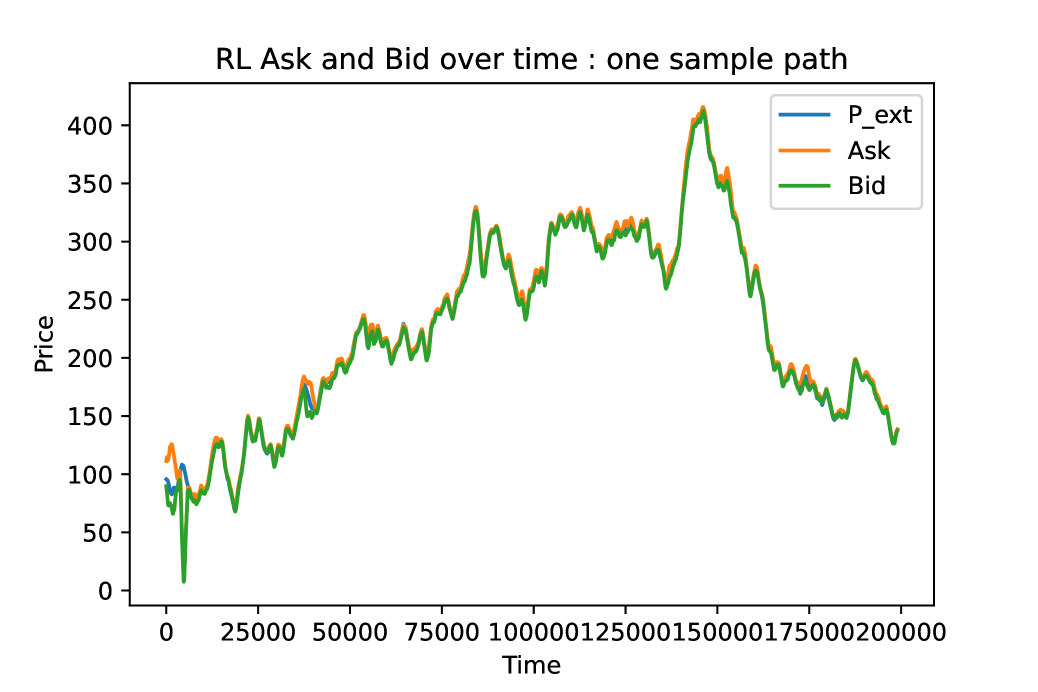
(a) $p_{ask}$, $p_{bid}$ and $p_{ext}$

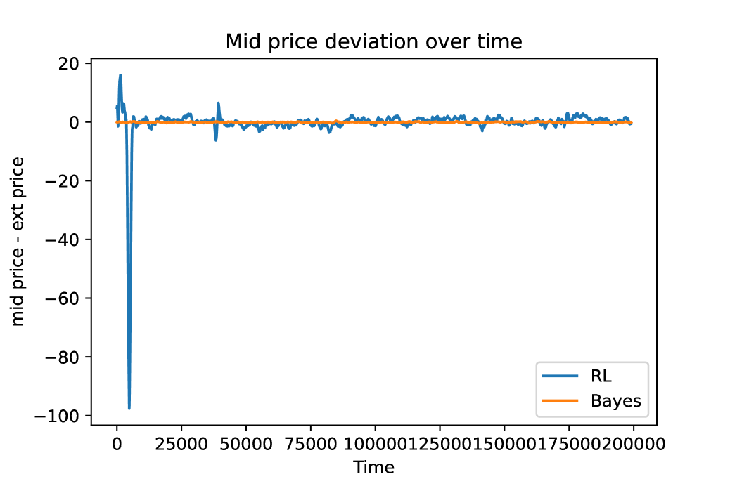
(b) Mid price deviation

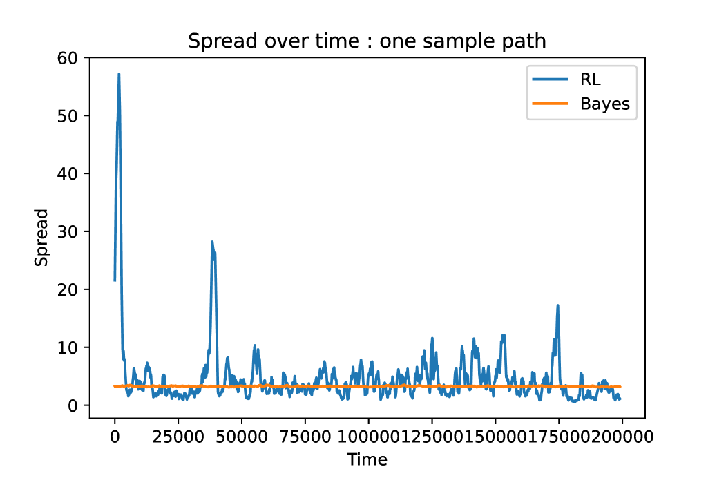
(c) Spread

Figure 7. The conjectured reward for the model-free algorithm trains the agent to track the external hidden price, eventually approaching the performance of the optimal Bayesian algorithm.

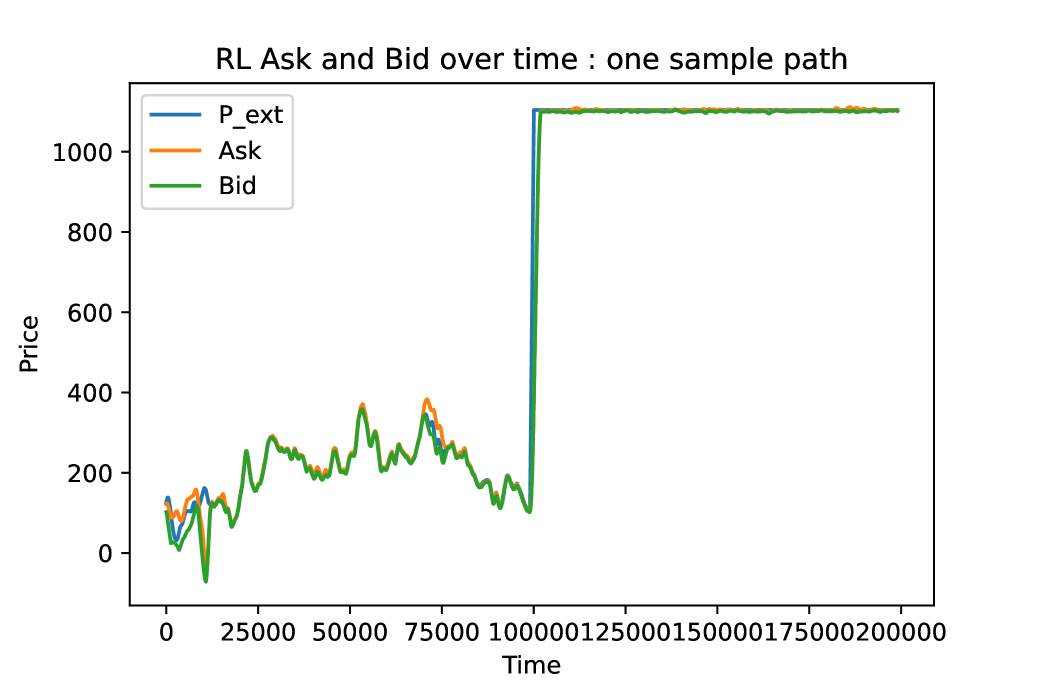
(a) $p_{ask}$, $p_{bid}$ and $p_{ext}$

(b) Mid price deviation

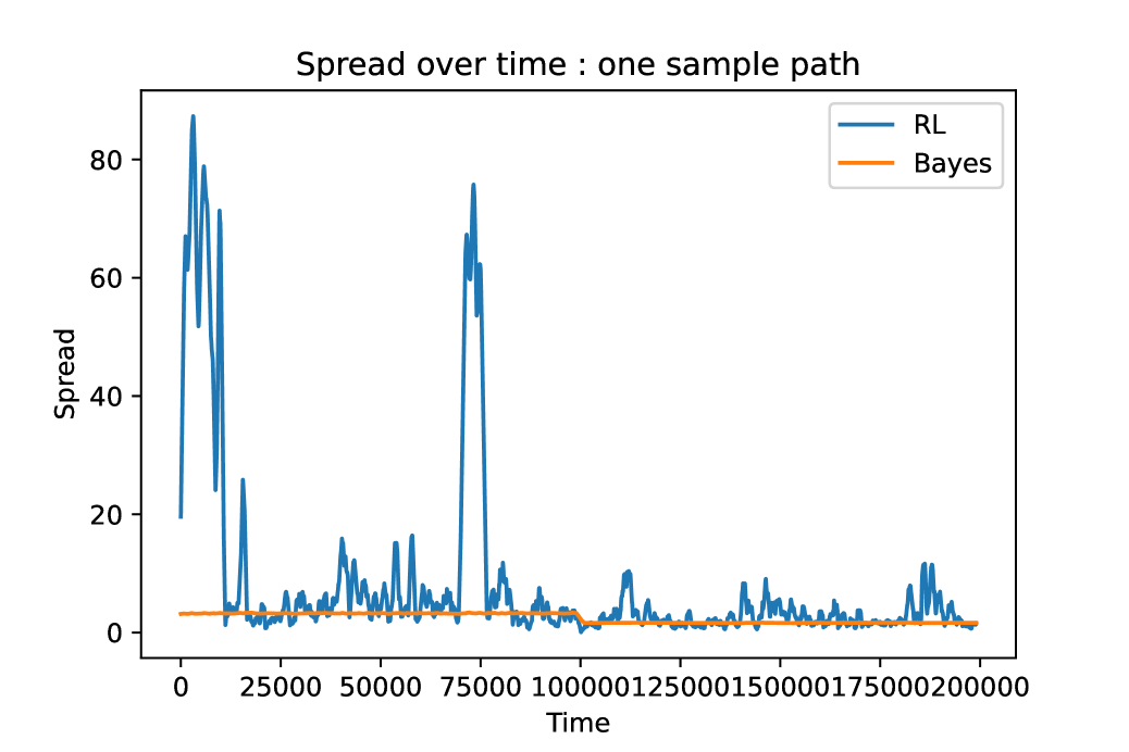
(c) Spread

Figure 8. The conjectured reward for the model-free algorithm trains the agent to track the external hidden price, even in the presence of large price jumps.

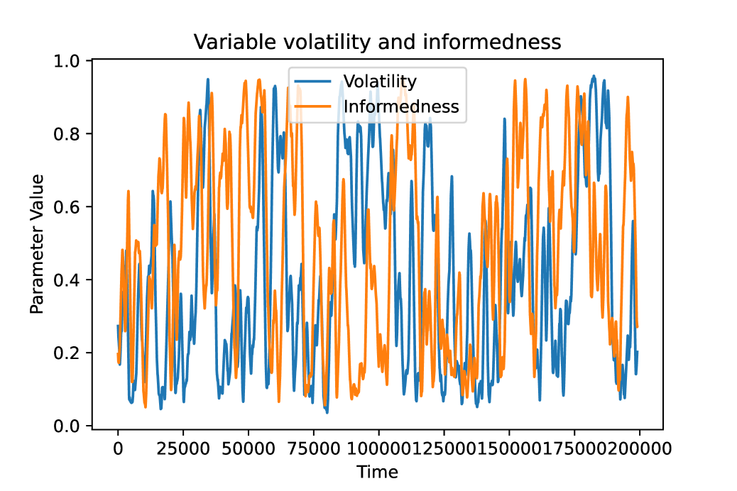
(a) Erratic changes in trader informedness and price volatility

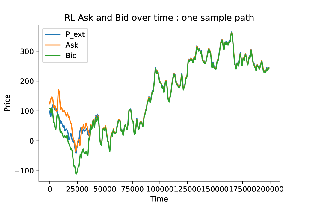
(b) Ask, Bid and $p_{ext}$

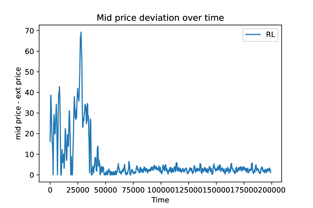
(c) Deviation from mid price

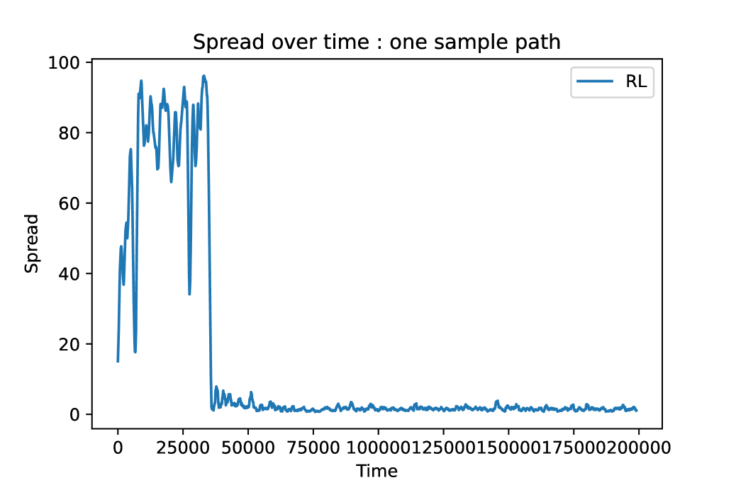
(d) Spread

Figure 9. The conjectured reward trains the agent to track the external hidden price, even in the presence of erratic changes in the market conditions

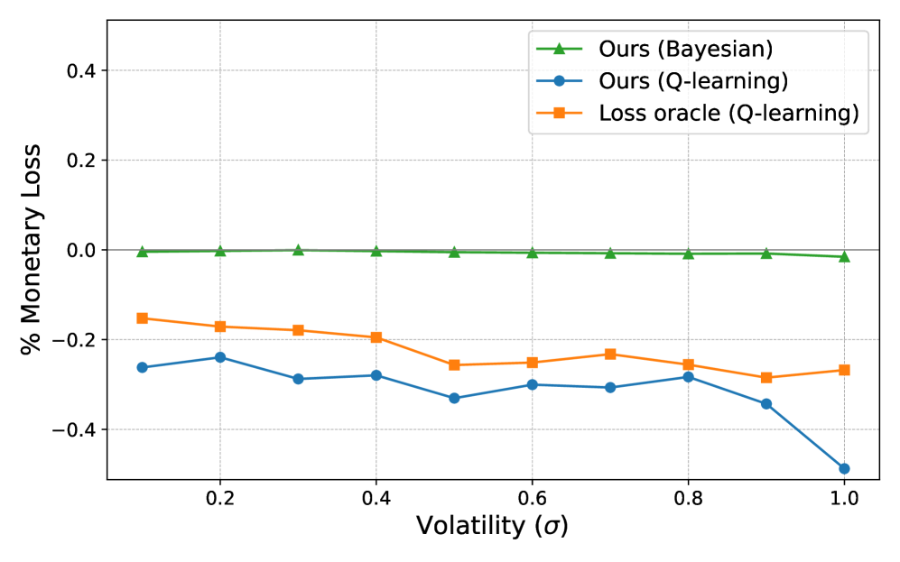
(a) Percentage monetary loss per trade of our market maker is comparable with the algorithm which has access to the loss oracle

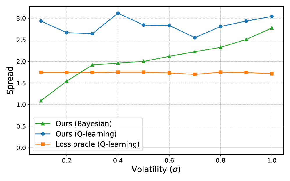
(b) Larger spread observed without access to the loss oracle

Figure 10. Algorithm 2 gives us comparable monetary loss per trade as running the algorithm with an oracle. The Bayesian algorithm gives loss close to zero, which is optimally efficient. The plots are against varying volatility for $\alpha=0.9$.

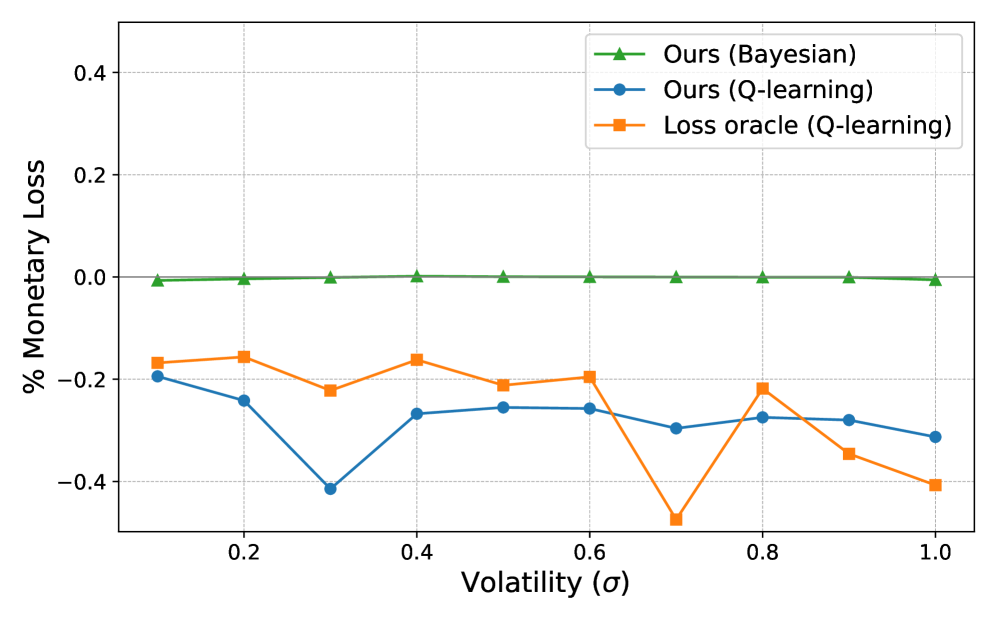
(a) Percentage monetary loss per trade of our market maker is comparable with the algorithm which has access to the loss oracle

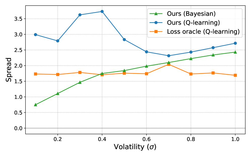
(b) Larger spread observed without access to the loss oracle

Figure 11. Algorithm 2 gives us comparable monetary loss per trade as running the algorithm with an oracle. The Bayesian algorithm gives loss close to zero, which is optimally efficient. The plots are against varying volatility for $\alpha=0.8$.

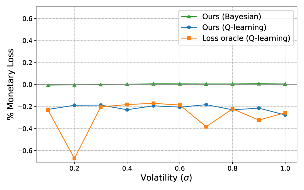
(a) Percentage monetary loss per trade of our market maker is comparable with the algorithm which has access to the loss oracle

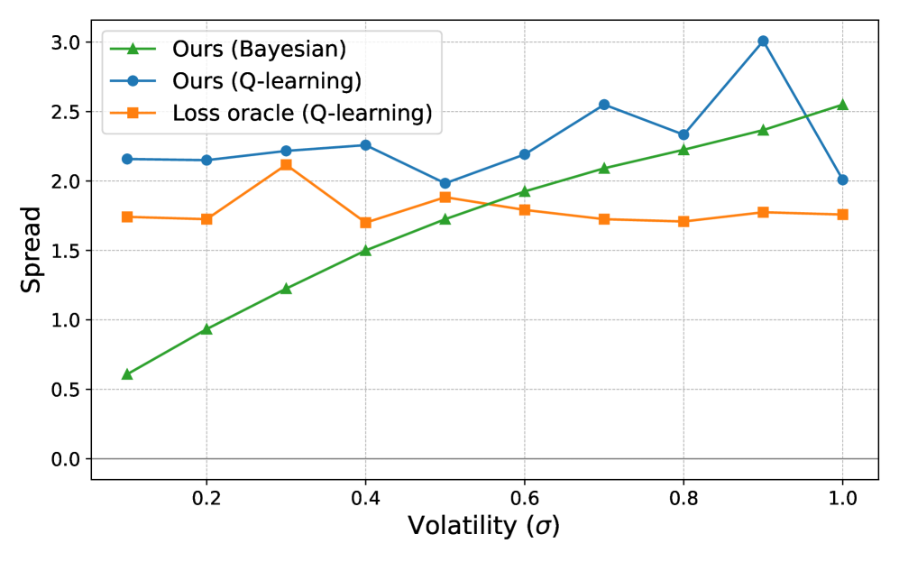
(b) Larger spread observed without access to the loss oracle

Figure 12. Algorithm 2 gives us comparable monetary loss per trade as running the algorithm with an oracle. The Bayesian algorithm gives loss close to zero, which is optimally efficient. The plots are against varying volatility for $\alpha=0.7$.

(a) Percentage monetary loss per trade of our market maker is comparable with the algorithm which has access to the loss oracle

(b) Larger spread observed without access to the loss oracle

Figure 13. Algorithm 2 gives us comparable monetary loss per trade as running the algorithm with an oracle. The Bayesian algorithm gives loss close to zero, which is optimally efficient. The plots are against varying volatility for $\alpha=0.6$.

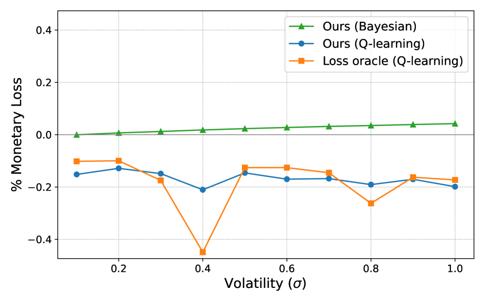
(a) Percentage monetary loss per trade of our market maker is comparable with the algorithm which has access to the loss oracle

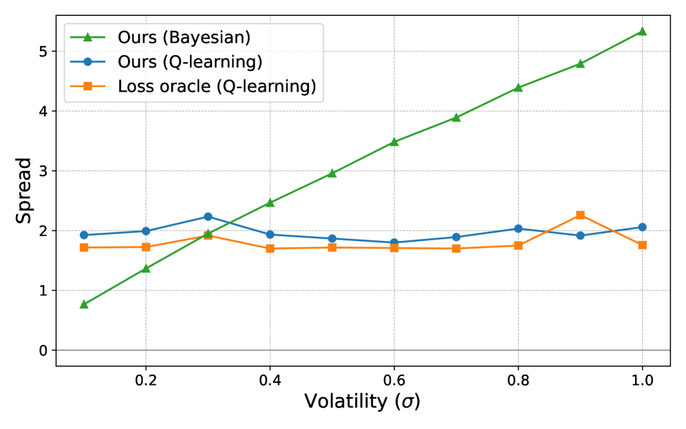
(b) Larger spread observed without access to the loss oracle

Figure 14. Algorithm 2 gives us comparable monetary loss per trade as running the algorithm with an oracle. The Bayesian algorithm gives loss close to zero, which is optimally efficient. The plots are against varying volatility for $\alpha=0.5$.

(a) Percentage monetary loss per trade of our market maker is comparable with the algorithm which has access to the loss oracle

(b) Larger spread observed without access to the loss oracle

Figure 15. Algorithm 2 gives us comparable monetary loss per trade as running the algorithm with an oracle. The Bayesian algorithm gives loss close to zero, which is optimally efficient. The plots are against varying volatility for $\alpha=0.4$.

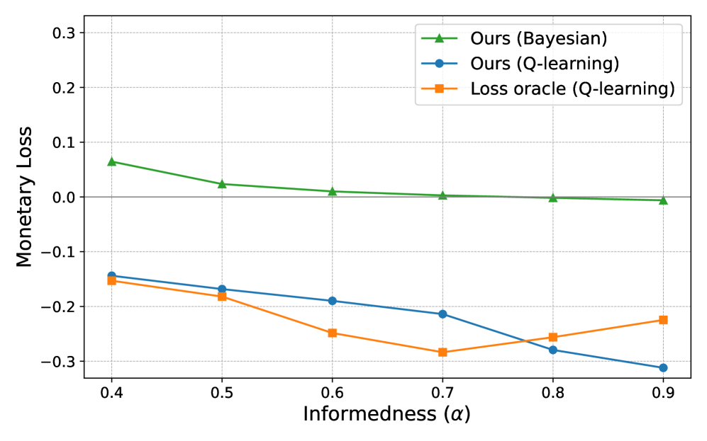
(a) Percentage monetary loss per trade of our market maker is comparable with the algorithm which has access to the loss oracle

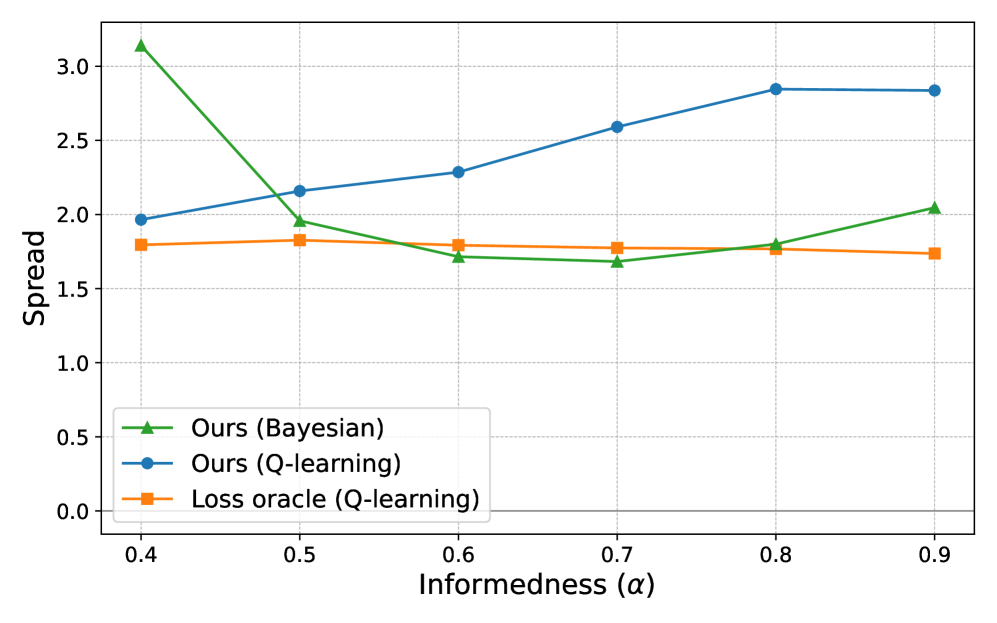
(b) Larger spread observed without access to the loss oracle

Figure 16. Algorithm 2 gives us comparable monetary loss per trade as running the algorithm with an oracle. The Bayesian algorithm gives loss close to zero, which is optimally efficient. The plots are against varying informedness $\alpha$, and are averaged over values of volatility $\sigma$.

References

- [1] Cowswap docs. https://docs.cow.fi/overview/coincidence-of-wants. Accessed: 2023-09.
- [2] Discrimination of toxic flow in uniswap v3. https://crocswap.medium.com/discrimination-of-toxic-flow-in-uniswap-v3-part-1-fb5b6e01398b. Accessed: 2023-09.
- [3] Dodo integrates chainlink live on mainnet, kickstarts the on-chain liquidity revolution. https://blog.dodoex.io/dodo-integrates-chainlink-live-on-mainnet-kickstarts-the-on-chain-liquidity-revolution-ee27e136e122. Accessed: 2023-09.
- [4] Eigenlayer whitepaper. https://docs.eigenlayer.xyz/overview/whitepaper. Accessed: 2023-09.
- [5] Flash loans aren’t the problem, centralized price oracles are. https://www.coindesk.com/tech/2020/11/11/flash-loans-arent-the-problem-centralized-price-oracles-are/. Accessed: 2023-09.
- [6] Front running, bots, slippage, oracle pricing errors: Amms are great, but there are problems. https://cointelegraph.com/magazine/trouble-with-crypto-automated-market-makers/. Accessed: 2023-09.
- [7] Optimism docs. https://community.optimism.io/. Accessed: 2023-09.
- [8] Optimistic rollups. https://ethereum.org/en/developers/docs/scaling/optimistic-rollups/. Accessed: 2023-09.
- [9] Order flow toxicity on dexes. https://ethresear.ch/t/order-flow-toxicity-on-dexes/13177. Accessed: 2023-09.
- [10] Peter johnson and sai nimmagadda. the relentless rise of stablecoins. brevan howard digital. https://digify.com/a/#/f/p/ef09be008ee64ab68bda4f0a558302a2. Accessed: 2023-09.
- [11] Random walk–1-dimensional, wolfram mathworld. https://mathworld.wolfram.com/RandomWalk1-Dimensional.html. Accessed: 2023-06.
- [12] Uniswap v3 core. https://uniswap.org/whitepaper-v3.pdf. Accessed: 2023-09.
- [13] Uniswap-v3 tvl comparison for stable coins vs non-stablecoins. https://defillama.com/protocol/uniswap-v3. Accessed: 2023-09.
- [14] Guillermo Angeris, Akshay Agrawal, Alex Evans, Tarun Chitra, and Stephen Boyd. Constant function market makers: Multi-asset trades via convex optimization, 2021.
- [15] Guillermo Angeris and Tarun Chitra. Improved price oracles. In Proceedings of the 2nd ACM Conference on Advances in Financial Technologies. ACM, oct 2020.
- [16] Guillermo Angeris, Alex Evans, and Tarun Chitra. When does the tail wag the dog? curvature and market making, 2020.
- [17] Jun Aoyagi. Liquidity provision by automated market makers, 2020.
- [18] Marco Avellaneda and Sasha Stoikov. High frequency trading in a limit order book. Quantitative Finance, 8:217–224, 04 2008.
- [19] Nicholas Chan and Christian Shelton. An electronic market-maker. 01 2001.
- [20] Dev Churiwala and Bhaskar Krishnamachari. Qlammp: A q-learning agent for optimizing fees on automated market making protocols, 2022.
- [21] Philip Daian, Steven Goldfeder, Tyler Kell, Yunqi Li, Xueyuan Zhao, Iddo Bentov, Lorenz Breidenbach, and Ari Juels. Flash boys 2.0: Frontrunning, transaction reordering, and consensus instability in decentralized exchanges, 2019.
- [22] Sanmay Das*. A learning market-maker in the glosten–milgrom model. Quantitative Finance, 5(2):169–180, 2005.
- [23] Sanmay Das and Malik Magdon-Ismail. Adapting to a market shock: Optimal sequential market-making. Advances in Neural Information Processing Systems, 21, 2008.
- [24] Shayan Eskandari, Mehdi Salehi, Wanyun Catherine Gu, and Jeremy Clark. SoK. In Proceedings of the 3rd ACM Conference on Advances in Financial Technologies. ACM, sep 2021.
- [25] Alex Evans, Guillermo Angeris, and Tarun Chitra. Optimal fees for geometric mean market makers, 2021.
- [26] Rafael Frongillo, Maneesha Papireddygari, and Bo Waggoner. An axiomatic characterization of cfmms and equivalence to prediction markets. arXiv preprint arXiv:2302.00196, 2023.
- [27] Lawrence R. Glosten and Paul R. Milgrom. Bid, ask and transaction prices in a specialist market with heterogeneously informed traders. Journal of Financial Economics, 14(1):71–100, 1985.
- [28] Mohak Goyal, Geoffrey Ramseyer, Ashish Goel, and David Mazières. Finding the right curve: Optimal design of constant function market makers, 2023.
- [29] SANFORD J. GROSSMAN and MERTON H. MILLER. Liquidity and market structure. The Journal of Finance, 43(3):617–633, 1988.
- [30] Lioba Heimbach, Eric Schertenleib, and Roger Wattenhofer. Risks and returns of uniswap v3 liquidity providers. In Proceedings of the 4th ACM Conference on Advances in Financial Technologies. ACM, sep 2022.
- [31] Thomas S. Y. Ho and Hans R. Stoll. The dynamics of dealer markets under competition. The Journal of Finance, 38(4):1053–1074, 1983.
- [32] Matt Hoffman, David M. Blei, Chong Wang, and John Paisley. Stochastic variational inference, 2013.
- [33] Harry Kalodner, Steven Goldfeder, Xiaoqi Chen, S. Matthew Weinberg, and Edward W. Felten. Arbitrum: Scalable, private smart contracts. In 27th USENIX Security Symposium (USENIX Security 18), pages 1353–1370, Baltimore, MD, August 2018. USENIX Association.
- [34] Albert S. Kyle. Continuous auctions and insider trading. Econometrica, 53(6):1315–1335, 1985.
- [35] Stefan Loesch, Nate Hindman, Mark B Richardson, and Nicholas Welch. Impermanent loss in uniswap v3, 2021.
- [36] Conor McMenamin, Vanesa Daza, and Bruno Mazorra. Diamonds are forever, loss-versus-rebalancing is not, 2022.
- [37] Jason Milionis, Ciamac C. Moallemi, and Tim Roughgarden. Automated market making and arbitrage profits in the presence of fees, 2023.
- [38] Jason Milionis, Ciamac C. Moallemi, and Tim Roughgarden. A myersonian framework for optimal liquidity provision in automated market makers, 2023.
- [39] Jason Milionis, Ciamac C. Moallemi, Tim Roughgarden, and Anthony Lee Zhang. Automated market making and loss-versus-rebalancing, 2022.
- [40] Volodymyr Mnih, Koray Kavukcuoglu, David Silver, Alex Graves, Ioannis Antonoglou, Daan Wierstra, and Martin Riedmiller. Playing atari with deep reinforcement learning, 2013.
- [41] Vijay Mohan. Automated market makers and decentralized exchanges: a defi primer, 12 2020.
- [42] Geoffrey Ramseyer, Mohak Goyal, Ashish Goel, and David Mazières. Augmenting batch exchanges with constant function market makers, 2023.
- [43] Rohan Tangri, Peter Yatsyshin, Elisabeth A. Duijnstee, and Danilo Mandic. Generalizing impermanent loss on decentralized exchanges with constant function market makers, 2023.
- [44] Christopher JCH Watkins and Peter Dayan. Q-learning. Machine learning, 8:279–292, 1992.
- [45] Jiahua Xu, Krzysztof Paruch, Simon Cousaert, and Yebo Feng. Sok: Decentralized exchanges (dex) with automated market maker (amm) protocols. ACM Comput. Surv., 55(11), feb 2023.