Modeling missing at random neuropsychological test scores using a mixture of binomial product experts

Abstract

Multivariate bounded discrete data arises in many fields. In the setting of longitudinal dementia studies, such data is collected when individuals complete neuropsychological tests. We outline a modeling and inference procedure that can model the joint distribution conditional on baseline covariates, leveraging previous work on mixtures of experts and latent class models. Furthermore, we illustrate how the work can be extended when the outcome data is missing at random using a nested EM algorithm. The proposed model can incorporate covariate information, perform imputation and clustering, and infer latent trajectories. We apply our model on simulated data and an Alzheimer’s disease data set.

and

1 Introduction

Modeling multivariate discrete data is a common problem across many fields such as social sciences, psychology, and ecology. For instance, in education research, discrete data arises from students’ test scores (Maydeu-Olivares and Liu, 2015), and in ecology, discrete data arises when the counts of a given animal population are measured over various areas and time periods (Anderson et al., 2019; Maslen et al., 2023). As the size of data sets continues to expand, missing data becomes increasingly prevalent (Kang, 2013), and it is common to have access to a rich set of discrete variables that is subject to missingness. Both the multivariate discreteness and the missingness alone can create modeling difficulties, but together, they present a unique challenge for statistical inference.

1.1 The National Alzheimer’s Coordinating Center database

Although the general problem statement is widely important, our work is primarily motivated by the analysis of neuropsychological test scores in the database of the National Alzheimer’s Coordinating Center (NACC). The NACC is an NIH/NIA-funded center that maintains the largest longitudinal database for Alzheimer’s disease in the United States. The NACC coordinates 33 Alzheimer’s Disease and Research Centers (ADRC) in the United States.

In the NACC data, we have 41,181 individuals with data collected from 2005 to 2019. There are more than 700 variables for each individual per year. These variables include demographic information, clinical assessments, and cognitive and lab test results. In this study, we are particularly interested in information regarding the neuropsychological tests. The neuropsychological tests are a set of examinations measuring an individual’s cognitive ability in four different domains: language, attention, executive function, and memory. The scores from these tests are important features for dementia research because they are not based on a clinician’s judgment. Similar to a conventional exam, the outcome of a neuropsychological test is a discrete number taking integer values and has a known range. Note that different tests have a different ranges. In our study, we consider eight neuropsychological test scores per individual.

The NACC database also includes the Clinical Dementia Rating (CDR) score with potential values 0, 0.5, 1, 2, 3. The CDR score is based on a clinician’s judgment on an individual’s cognitive ability and is the standard procedure to determine whether someone has dementia or not. A CDR score 0 refers to cognitively normal, a score 0.5 is called a mild cognitive impairment (MCI) state, and a score of at least 1 refers to dementia. Note that the CDR score is all based on a clinician’s judgment, which is very different from the neuropsychological tests (exam-based).

1.2 Research questions

Because the ranges of exams are generally large (30 to 300), it is infeasible to nonparametrically model the joint distribution of the eight test scores. Moreover, we have demographic variables such as education, age, and sex. It is a nontrivial problem to study the relation between these demographic variables and the test scores. Furthermore, the existence of missing test scores among certain individuals further compounds the complexity of the overall analysis. In this paper, our primary focus centers on addressing the following research questions:

1. Finding a feasible and interpretable model for multiple discrete outcomes with missing values. As mentioned before, our data contains multiple dependent discrete variables with missing values. We need to design a proper model to model the dependency among discrete variables and deal with the missing data problem. We also need an estimation and inference procedure that quantifies the uncertainty in the model while properly accounting for the missing data in a statistically principled way.

2. Discovering latent groups of individuals using neuropsychological tests. Clinicians have developed a set of rules to categorize individuals into different clinical groups (normal cognition, MCI, and dementia). However, this rule is based on clinical judgments and does not involve any neuropsychological information. Clustering has been of interest to the dementia research community (Alashwal et al., 2019). Thus, an ideal model should be able to cluster individuals into groups using neuropsychological test scores that represent multiple cognitive domains of interest.

3. Investigating the association between neuropsychological tests and other variables. It is often of a lot of interest to study how neuropsychological tests are associated with demographic variables or clinical judgments. For instance, there is a hypothesis that people with a higher education are more resilient to cognitive decline as a form of cognitive reserve (Meng and D’Arcy, 2012; Thow et al., 2018). We also want to use the NACC data to test this hypothesis.

1.3 Literature review

We provide some background on the current research in the Alzheimer’s disease and statistics methodology literature.

1.3.1 Dementia-related research

Multiple outcome variables are common in dementia-related research, but there is no clear widespread solution to the modeling problem. In some previous methods in the Alzheimer’s disease literature, multiple test scores are standardized and averaged into a single holistic score for an individual (Boyle et al., 2018). This turns the multiple outcome problem into a single outcome problem and ignores the dependence structure. Mjørud et al. (2014) examined variables associated with multiple quality-of-life related discrete outcomes and performed univariate regression on each outcome. Dimension reduction is also commonly used to reduce the number of outcome variables (Yesavage et al., 2016; Qiu et al., 2019), but this can lead to loss of interpretability as any downstream analysis is not using the original variables. Missing data is often ignored completely or when accounted for, single imputation methods or an off-the-shelf imputation approach are typically used (Brenowitz et al., 2017; Qiu et al., 2019).

Clustering has also become increasingly valuable in the dementia research community (Alashwal et al., 2019). For example, Escudero, Zajicek and Ifeachor (2011) used the $K$-means algorithm to divide subjects into pathologic and non-pathologic groups to study the early detection of Alzheimer’s disease. Tosto et al. (2016) used $K$-means on a subset of NACC data to identify subgroups within Alzheimer’s disease patients to understand the heterogeneity of the disease. Several papers also described model-based clustering approaches. For example, De Meyer et al. (2010) clustered biomarker data using a simple two-component Gaussian mixture model for early detection of Alzheimer’s disease. Qiu et al. (2019) used neuropsychological test scores from a smaller data set than ours, imputing missing data using single imputation methods and the mice R package (van Buuren and Groothuis-Oudshoorn, 2011). Then, they applied principal components analysis before finally, using a Gaussian mixture model for clustering. In our work, we choose to model the raw test scores to avoid loss of information and preserve more interpretability. It is crucial to be cautious when employing single imputation methods or off-the-shelf packages, as they can potentially lead to an underestimation of the uncertainty associated with missing data, and the underlying assumptions regarding missing data may remain unclear.

Additionally, the cognitive reserve hypothesis emerged several decades ago when it was observed that after autopsies, some individuals with no dementia symptoms had brains that exhibited advanced Alzheimer’s pathology (Katzman et al., 1989). Researchers hypothesized that some activities in life may provide individuals with a given resilience to cognitive decline, which is known as the cognitive reserve hypothesis. As such, there is deep interest in discovering the association between various covariates and dementia (Zhang et al., 1990; Stern, 2012; Meng and D’Arcy, 2012; Thow et al., 2018).

1.3.2 Methodology research

This paper sits at the intersection of multiple subfields of statistics including latent variable modeling, missing data, and clustering. The latent class model was first proposed by Goodman (1974) for the purpose of modeling multivariate discrete data. The basic form of the latent class model is of a mixture of multivariate multinomials. When the number of levels of the discrete random variable is large, this can lead to a large number of parameters (Bouveyron et al., 2019). There has been much work studying many aspects of the latent class model including the identifiability (Gyllenberg et al., 1994; Carreira-Perpinan and Renals, 2000; Allman, Matias and Rhodes, 2009; Gu and Xu, 2020) and incorporation of covariates (Huang and Bandeen-Roche, 2004; Vermunt, 2010; Ouyang and Xu, 2022). The traditional latent class model has been extended in various forms such as a mixture of Rasch models (Rost, 1990) and a mixture of item response models (McParland and Gormley, 2013).

The mixture of experts models are closely related to the mixture model framework and the latent class model (Jacobs et al., 1991). It generalizes the standard mixture model by allowing the parameters to potentially depend on covariates (Gormley and Frühwirth-Schnatter, 2018). The increased flexibility of the models is associated with a large increase in number of parameter. Many estimation procedures have been explored including those based on an EM approach (Jacobs et al., 1991; Jordan and Jacobs, 1993), an EMM approach (Gormley and Murphy, 2008), or a Bayesian framework (Bishop and Svenskn, 2002; Fruhwirth-Schnatter and Kaufmann, 2008).

Clustering has previously been explored in combination with missing data. Lee and Harel (2022) proposed a two stage clustering framework by first clustering multiply imputed data sets individually and then, obtaining a final clustering by clustering the set of cluster centers obtained over all imputed data sets. In previous research on model-based clustering with missing data, Serafini, Murphy and Scrucca (2020) employed the EM algorithm and Monte Carlo methods to estimate Gaussian mixture models in the presence of missing at random data. Sportisse et al. (2023) addressed model-based clustering under missing-not-at-random assumptions, employing a likelihood-based approach and EM algorithm. These methods addressed the clustering problem but did not use covariates or discuss quantifying the uncertainty of the parameters. Since our method is motivated by the statistical analysis of Alzheimer’s disease, handling both of these is critical to our work.

1.4 Outline

Our paper is organized as follows. Section 2 presents a detailed description of our mixture of binomial product experts model. The handling of missing data is discussed in Section 3, where we describe the fitting of the model under a nonmonotone missing at random assumption. In Section 4, we delve into the process of inference, specifically in constructing confidence intervals for the parameters of interest. We outline how to perform clustering in Section 5. In Section 6, we apply our method to an Alzheimer’s disease data set, which motivates our model formulation. Finally, Section 7 concludes the paper with a discussion of the results. In the Appendix, we include further details on derivations and proofs (Appendices A and F), identification theory (Appendix B), code implementation (Appendix C), simulations (Appendix D), comments on model selection (Appendix E), and more real data analysis (Appendix G). We provide a code implementation of our method in an R package, which is available at https://github.com/danielsuen/mixturebpe.

2 Mixture of Binomial Product Experts

2.1 A latent class model for neuropsychological test scores

Suppose we have $n$ IID observations, indexed by $i=1,\ldots,n$. Let $\textbf{X}_{i}=(X_{i,1},X_{i,2},\ldots,X_{i,p})^{\top}\in\mathcal{X}\subset\mathbb{R}^{p}$ be the covariates and $\textbf{Y}_{i}=(Y_{i,1},Y_{i,2},\ldots,Y_{i,d})^{\top}\in\mathcal{Y}\subset\mathbb{Z}^{d}$ be the outcome variables of interest, where $\mathcal{Y}$ is a bounded discrete set. In the present study, $\textbf{Y}_{i}$ represents the neuropsychological test scores of individual $i$ for a total of $d$ total tests, but this framework can be applied to other problems as well. In the paper, for notational convenience, we may elect to drop the index $i$ to simplify notation and refer to the generic random variable that is not associated with a specific individual. The $j$th test score/outcome variable $Y_{j}$ belongs to the set $\{0,1,2,\ldots,N_{j}\}$. We assume that the covariates are always observed and that only the outcomes may be subject to missingness.

We start with a simpler scenario in which the data is completely observed (no absence of any outcome variables). The more complicated setting with missing outcome variables is addressed in Section 3. When we have multiple discrete outcome variables, the nonparametric approach is not feasible due to the curse of dimensionality. To see this, suppose we have four outcome variables, and each outcome variable has ten possible values. The joint distribution has a dimension of $10^{4}$, surpassing the order of magnitude of moderately sized samples. This motivates to use a parametric model.

To model the dependency among discrete variables, we consider a mixture model, which is based on the idea of the latent class model (LCM). Originally presented in its modern form by Goodman (1974), the latent class model takes the form of the following mixture of multivariate multinomials distribution

$$p(y;\theta)=\sum_{k=1}^{K}w_{k}p_{k}(y;\theta_{k})=\sum_{k=1}^{K}w_{k}\prod_{j=1}^{d}p_{k,j}(y_{j};\theta_{k,j}),$$ (2.1)

where $p_{k,j}$ denotes a multinomial with $\theta_{k,j}$ being its the parameter and the $w_{k}$’s are probability weights for each component such that $\sum_{k}w_{k}=1$ and $w_{k}>0$ for all $k$. As $p_{k,j}$ is a multinomial distribution, $\theta_{k,j}$ refers to vector of probabilities (one for each level of $Y_{j}$) that sum to 1.

Let $Z$ denote the component assignment such that $Z=\ell$ if and only if the associated observation is generated from mixture component $\ell$. Namely, $P(Y=y|Z;\theta)=\prod_{j=1}^{d}p_{k,j}(y_{j};\theta_{k,j})$. By construction, the latent class model implicitly assumes for $j\neq j^{\prime}$, the variables $Y_{j}$ and $Y_{j^{\prime}}$ are conditionally independent given the latent class $Z$. This is known as the local independence assumption. While they are conditionally independent, the variables $Y_{j}$ and $Y_{j^{\prime}}$ are allowed to depend marginally for $j\neq j^{\prime}$. The local independence assumption makes it convenient to calculate the conditional distributions, which are used in Section 3 when we discuss imputation. Some effort has been made to relax the local independence assumption such as mixtures of log-linear models (Bock, 1994) and hiearchical latent class models (Zhang, 2004; Chen et al., 2012), but these are have not been as widely adopted due to the increase in the number of parameters.

Throughout this paper, we will refer to the data set containing tuples of the form $(\textbf{X},\textbf{Y})$ as the latent incomplete (LI) data and the data set containing tuples of the form $(\textbf{X},\textbf{Y},Z)$ as the latent complete (LC) data. In the setting of no missing data, the latent incomplete data is what we typically have access to, but this is often insufficient for direct model fitting due to the unobserved latent variable $Z$. We will show that one can estimate the model parameters using an EM algorithm with the latent incomplete data. We use this nomenclature to avoid confusion in Section 3 when we encounter the traditional type of missingness with the outcome variables.

There has been previous work to incorporate covariates in the latent class model (Huang and Bandeen-Roche, 2004; Vermunt, 2010). This is related to the mixture of experts models that arose from the machine learning literature (Jacobs et al., 1991; Jordan and Jacobs, 1993; Yuksel, Wilson and Gader, 2012). These models generalize the classical mixture model formulation by allowing the model parameters $w_{k}$ and $\theta_{k}$ to depend on covariates. The simple mixture of experts model (Gormley and Frühwirth-Schnatter, 2018) takes the following form

$$p(y|x;\bm{\theta})=\sum_{k=1}^{K}w_{k}(x;\beta_{k})p_{k}(y;\theta_{k}),$$

where $\beta_{k}$ is introduced to allow the weights to depend on covariates. As written, the covariates only adjust the weights placed on each mixture component but do not affect the parameters of the individual component distribution.

To apply these ideas to the neuropsychological data, we combine the mixture of experts and LCM, leading to the following mixture of binomial product experts

$$p(y|x;\bm{\beta},\bm{\theta})=\sum_{k=1}^{K}w_{k}(x;\beta_{k})\underbrace{\prod_{j=1}^{d}\underbrace{\binom{N_{j}}{y_{j}}(\theta_{k,j})^{y_{j}}(1-\theta_{k,j})^{N_{j}-y_{j}}}_{p_{k,j}(y_{j};\theta_{k,j})}}_{p_{k}(y;\theta_{k})},$$ (2.2)

where $w_{k}(x;\beta_{k})=\exp(\beta_{k}^{\top}\cdot(1,x))/(\sum_{k^{\prime}\in[K]}\exp(\beta_{k^{\prime}}^{\top}\cdot(1,x)))$ is from the multiple-class logistic regression model. Like in the classical LCM, we utilize the local independence assumption as each mixture decomposes as a product of binomials. However, there is a critical difference between our model and the classical LCM. We use the binomial distribution instead of the multinomial distribution, and this leads to large reduction in the number of parameters. Since test scores are ordered variables, we expect the reduction to a binomial distribution to be reasonable as scores further away from the mean score can be less likely. Similar to the simple mixture of experts model, each mixture weight depends on covariates.

Here we will treat $k=1$ as the reference group, so $\beta_{1}$ is the vector of all $0$ by assumption and does not need to be estimated. For $k\in\{2,3,\ldots,K\}$, $\beta_{k}\in\mathbb{R}^{p+1}$, and for $k\in[K]$, $\theta_{k}\in\mathbb{R}^{d}$, we assume that the $w_{k}$ utilize the logistic function, but it is possible to use other link functions such as the probit and other monotonic functions (Ouyang and Xu, 2022). In our work, the outcome variables are neuropsychological test scores, and we treat the latent groups as subgroups of the population of varying cognitive ability. We interpret the $\bm{\theta}$’s as attributes of population-level groups and do not allow them to depend on covariates. We expect that the population can be divided into subgroups of varying cognitive ability, which is summarized by $\bm{\theta}$. Since the weights $w_{k}(x;\beta_{k})$ depend on covariates, every individual has their own weights associated with each population-level group. A side product of this assumption is that this reduces model complexity. Because the outcome variables are test scores, we can also interpret the quantity $N_{j}\cdot\theta_{k,j}$ as the mean of the $j$th test score of the $k$th latent group, and this is useful as a summary statistic for a given latent class.

Binomial product distributions have previously arisen in the literature. One such application was for modeling test scores for spatial tasks in child development in Thomas, Lohaus and Brainerd (1993), but they considered a fairly limited setting with no covariates, two components, and two outcome variables. Binomial product and Poisson product distributions have also been used in the statistical ecology literature to model species abundance (Kéry, Royle and Schmid, 2005; Haines, 2016; Brintz, Fuentes and Madsen, 2018). These settings differ from ours because they often treat the total number counts $N_{j}$ as a random quantity. To our knowledge, our paper is the first time binomial products has been used to analyze neuropsychological test score data while incorporating covariates.

Note that for $k$-th component, $\beta_{k}\in\mathbb{R}^{p+1}$ and $\theta_{k}\in\mathbb{R}^{d}$. So, there are $(K-1)(p+1)$ parameters associated with the covariates $\bm{\beta}$ and $Kd$ parameters associated with $\bm{\theta}$ and a total of $K(p+d+1)-p-1$ parameters for the whole model. Thus, for fixed covariate and outcome dimensions, the number of parameters grows linearly in $K$.

2.2 Model fitting

We now describe our procedure of fitting the model. An intuitive approach is to estimate the parameters via the maximum likelihood approach. However, computing the maximum likelihood estimator (MLE) is a nontrivial task because the latent incomplete log-likelihood is not concave (Lemma 2.1). Thus, obtaining a closed-form solution for the maximum likelihood estimator by taking a derivative with respect to the parameter is not possible. To see this, let $\textbf{X}_{1:n}=(\textbf{X}_{1},\ldots,\textbf{X}_{n})$ and $\textbf{Y}_{1:n}=(\textbf{Y}_{1},\ldots,\textbf{Y}_{n})$ be the covariates and outcome variables of all $n$ individuals. Then we have the following result.

Lemma 2.1 (Nonconcavity of the LI log-likelihood function).

The latent incomplete log-likelihood function

$$\ell_{\text{LI},n}(\beta,\theta;\textbf{X}_{1:n},\textbf{Y}_{1:n}) =\log\left(\prod_{i=1}^{n}\left(\sum_{k=1}^{K}w_{k}(\textbf{X}_{i};\beta_{k})p_{k}(\textbf{Y}_{i};\theta_{k})\right)\right)$$

$$=\sum_{i=1}^{n}\log\left(\sum_{k=1}^{K}w_{k}(\textbf{X}_{i};\beta_{k})p_{k}(\textbf{Y}_{i};\theta_{k})\right).$$

is not concave.

The proof is in Appendix F.1. Due to Lemma 2.1, maximizing the latent incomplete log-likelihood function directly is not straightforward. Here is an interesting insight from the mixture model literature: if we had access to the latent class label, then the maximum likelihood estimator would be easy to construct. This insight motivates us to develop an EM algorithm (Dempster, Laird and Rubin, 1977) by augmenting the observed data with the true component label $Z$ to calculate the MLE for $(\bm{\beta},\bm{\theta})$. For each $i=1,\ldots,n$, let $Z_{i}=\ell$ if the $i$-th observation comes from mixture component $\ell$. Such data augmentation allows one to bypass the problem of taking the logarithm of a sum. The latent complete (LC) log-likelihood function writes as

$$\ell_{\text{LC},n} (\beta,\theta;\textbf{X}_{1:n},\textbf{Y}_{1:n},\textbf{Z}_{1:n})=\log\left(\prod_{i=1}^{n}\prod_{k=1}^{K}\left(w_{k}(\textbf{X}_{i};\beta_{k})p_{k}(\textbf{Y}_{i};\theta_{k})\right)^{1(Z_{i}=k)}\right)$$

$$=\sum_{i=1}^{n}\sum_{k=1}^{K}1(Z_{i}=k)\log w_{k}(\textbf{X}_{i};\beta_{k})+\sum_{i=1}^{n}\sum_{k=1}^{K}1(Z_{i}=k)\log p_{k}(\textbf{Y}_{i};\theta_{k}).$$ (2.3)

In the EM algorithm, we start from an initial guess $(\hat{\bm{\beta}}^{(0)},\hat{\bm{\theta}}^{(0)})$ and iterate between an expectation step (E-step) and a maximization step (M-step) to update our guess until convergence. Let $t$ denote the $t$th iteration of the EM algorithm. In the E-step, we compute the expected value of the complete log-likelihood $\ell_{\text{LC}}(\bm{\beta},\bm{\theta};\textbf{X},\textbf{Y},\textbf{Z})$ conditional on the observed data X and Y. The expected value of the latent complete log-likelihood given the observed data forms the $Q$ function in the EM algorithm

$$Q_{\text{LC}}(\bm{\beta},\bm{\theta}|\textbf{X},\textbf{Y};\hat{\bm{\beta}}^{(t)},\hat{\bm{\theta}}^{(t)}):=\mathbb{E}[\ell_{\text{LC}}(\bm{\beta},\bm{\theta};\textbf{X},\textbf{Y},Z)|\textbf{X},\textbf{Y};\hat{\bm{\beta}}^{(t)},\hat{\bm{\theta}}^{(t)}].$$

In practice, we do not have access to the true expectation, so we work with the sample analogue $Q_{\text{LC},n}$. The sample analogue can be expressed as

$$Q_{\text{LC},n}(\bm{\beta},\bm{\theta}|\textbf{X}_{1:n},\textbf{Y}_{1:n};\hat{\bm{\beta}}^{(t)},\hat{\bm{\theta}}^{(t)})$$

$$:=\frac{1}{n}\sum_{i=1}^{n}\sum_{k=1}^{K}\hat{\pi}_{k}^{(t)}(\textbf{X}_{i},\textbf{Y}_{i})\log w_{k}(\textbf{X}_{i};\beta_{k})+\frac{1}{n}\sum_{i=1}^{n}\sum_{k=1}^{K}\hat{\pi}_{k}^{(t)}(\textbf{X}_{i},\textbf{Y}_{i})\log p_{k}(\textbf{Y}_{i};\theta_{k}),$$ (2.4)

where

$$\hat{\pi}_{k}^{(t)}(\textbf{X}_{i},\textbf{Y}_{i}):=P(Z=k|\textbf{X}_{i},\textbf{Y}_{i};\hat{\bm{\beta}}^{(t)},\hat{\bm{\theta}}^{(t)})=\frac{w_{k}(\textbf{X}_{i};\hat{\beta}_{k}^{(t)})p_{k}(\textbf{Y}_{i};\hat{\theta}_{k}^{(t)})}{\sum_{k^{\prime}=1}^{K}w_{k^{\prime}}(\textbf{X}_{i};\hat{\beta}_{k^{\prime}}^{(t)})p_{k^{\prime}}(\textbf{Y}_{i};\hat{\theta}_{k^{\prime}}^{(t)})}$$ (2.5)

is the weight of observation $(\textbf{X}_{i},\textbf{Y}_{i})$ for the $k$th mixture component.

Since the latent-complete log-likelihood function (2.3) decomposes as the sum of a function of $\bm{\beta}$ and a function of $\bm{\theta}$, the maximization step of the EM algorithm is separable. Note that since $w_{k}$ and $p_{k}$ are logistic regression and binomial product models, respectively, one can apply standard off-the-shelf model fitting procedures after reweighting each observation $i$ by $\pi_{k}^{(t)}(\textbf{X}_{i},\textbf{Y}_{i})$. In the maximization step, the new estimate for $\bm{\theta}$ is updated as follows for each $k\in[K]$ and $j\in[d]$,

$$\hat{\theta}^{(t+1)}_{k,j}:=\dfrac{\sum_{i=1}^{n}\frac{Y_{i,j}}{N_{j}}\hat{\pi}_{k}^{(t)}(\textbf{X}_{i},\textbf{Y}_{i})}{\sum_{i=1}^{n}\hat{\pi}_{k}^{(t)}(\textbf{X}_{i},\textbf{Y}_{i})},$$ (2.6)

which is simply the standard MLE formed by the sample proportion, reweighted by $\hat{\pi}_{k}^{(t)}(\textbf{X}_{i},\textbf{Y}_{i})$. We update our estimate of $\beta_{k}$ by fitting a multi-class logistic regression by reweighting each corresponding observation by $\hat{\pi}_{k}^{(t)}(\textbf{X}_{i},\textbf{Y}_{i})$. This is equivalent to regressing the variable $W^{(t)}$ on the covariates $X$, where $W_{i}^{(t)}=(\hat{\pi}_{1}^{(t)}(\textbf{X}_{i},\textbf{Y}_{i}),\ldots,\hat{\pi}_{K}^{(t)}(\textbf{X}_{i},\textbf{Y}_{i}))\in S^{K-1}$ for all $i$, where $S^{K-1}$ is the $(K-1)$th probability simplex. Note that this is not the standard logistic regression because the outcome variable belongs to a probability simplex. This logistic regression can still be fit using gradient descent in standard R packages.

Require: $\{(\textbf{X}_{i},\textbf{Y}_{i})\}_{i=1}^{n}$, $(\hat{\bm{\beta}}^{(0)},\hat{\bm{\theta}}^{(0)})$

1:Start with an initial guess $(\hat{\bm{\beta}}^{(0)},\hat{\bm{\theta}}^{(0)})$.

2:Initialize the iteration step $t=0$.

3:repeat

4:     Compute the weights $\hat{\pi}_{k}^{(t)}(\textbf{X}_{i},\textbf{Y}_{i})$ for all observations $i$ and mixture components $k$ using (2.5).

5:     Form the probability vector $W_{i}^{(t)}=(\hat{\pi}_{1}^{(t)}(\textbf{X}_{i},\textbf{Y}_{i}),\ldots,\hat{\pi}_{K}^{(t)}(\textbf{X}_{i},\textbf{Y}_{i}))$ for each $i$.

6:     Update $\hat{\bm{\theta}}^{(t+1)}$ using (2.6).

7:     Update $\hat{\bm{\beta}}^{(t+1)}$ by fitting a logistic regression model of $W^{(t)}$ on X.

8:     Update $t\leftarrow t+1$.

9:until Convergence

10:Let $\hat{\bm{\beta}}=\lim_{t\to\infty}\hat{\bm{\beta}}^{(t)}$ and $\hat{\bm{\theta}}=\lim_{t\to\infty}\hat{\bm{\theta}}^{(t)}$.

11:return $(\hat{\bm{\beta}},\hat{\bm{\theta}})$

Algorithm 1 Fitting the mixture model via EM

Algorithm 1 describes the process of fitting the mixture of binomial products experts model in the presence of completely observed covariate and outcome data. The EM algorithm is not guaranteed to converge to the global maximizer. In practice, we run Algorithm 1 many times with multiple random initial guesses to explore the parameter space sufficiently and choose the parameter estimate from all of them that maximizes the log-likelihood.

3 Missingness in the Outcome Variables

A challenge in the NACC’s neuropsychological data is the missingness in the outcomes. To properly describe the missing data problem, we first introduce some additional notation. Let $\textbf{R}_{i}=(R_{i,1},R_{i,2},\ldots,R_{i,d})^{\top}\in\mathcal{R}\subseteq\{0,1\}^{d}$ be the random binary vector that denotes the missing pattern associated with individual $i$. Element $R_{i,j}$ of the binary vector $\textbf{R}_{i}$ is $1$ if and only if $Y_{i,j}$ is observed. For a given pattern $r\in\mathcal{R}$, let $\textbf{Y}_{i,r}=(Y_{i},j:r_{i,j}=1)$ denote the observed variables and $\textbf{Y}_{i,\bar{r}}=(Y_{i,j}:r_{i,j}=0)$ denote the missing variables. For example, when $d=4$ and $r=1001$, then $\textbf{Y}_{i,r}=(Y_{i,1},Y_{i,4})$ and $\textbf{Y}_{i,\bar{r}}=(Y_{i,2},Y_{i,3})$. Similarly, for observation $i$ with random missing pattern $\textbf{R}_{i}$, denote $\textbf{Y}_{i,\textbf{R}_{i}}$ and $\textbf{Y}_{i,\bar{\textbf{R}}_{i}}$ as the observed and missing outcome variables for the $i$th observation, respectively. We place no restrictions on the set of possible patterns $\mathcal{R}$, allowing the pattern to be nonmonotone. Since $|\mathcal{R}|\leq 2^{d}$, missingness can easily become an exponentially complex problem in the dimension of the outcome variables.

In contrast to the previous section, we will use the term fully complete (FC) to refer to a data set containing IID tuples of the form $(\textbf{X},\textbf{Y},Z,\textbf{R})$. We call a data set containing IID observations of the form $(\textbf{X},\textbf{Y}_{\textbf{R}},\textbf{R})$ as the observed data. Note that the observed data now has two kinds of incompleteness/missingness: incompleteness in the latent class variable (due to mixture models) and missingness in the outcomes. As the case with the latent complete data, we also do not have access to the fully complete data. We collect all of the observed outcome variables in one tuple $\textbf{Y}_{1:n,\textbf{R}_{1:n}}=(\textbf{Y}_{1,\textbf{R}_{1}},\textbf{Y}_{2,\textbf{R}_{2}},\ldots,\textbf{Y}_{n,\textbf{R}_{n}})$.

3.1 Missing at random and an imputation strategy

Rubin (1976) outlined three types of missingness mechanisms: missing completely at random (MCAR), missing at random (MAR), and missing not at random (MNAR). Missing completely at random assumes that the missingness of the variable is independent of all variables in the data. Missing at random assumes that the missingness of a variable can only depend on observed variables. Missing not at random assumes that the missingness of a variable can depend on the value of the variable subject to missingness.

In the MCAR data, model fitting is straightforward because one can run Algorithm 1 on the complete cases, and the estimates of the parameters will be consistent. However, MCAR assumes that the missingness is irrelevant to observed outcomes, which is clearly false in the NACC data as a common reason to miss some test scores is that the individual was too sick to finish the test. Therefore, we consider the MAR assumption. Formally, the definition of missing at random (MAR) is as follows.

Definition 3.1 (Missing at random).

The outcome variables Y are missing at random (MAR) if the probability of missingness is dependent only on the variables that are observed for the given pattern. This assumption writes as

$$P(\textbf{R}=r|\textbf{X},\textbf{Y})\stackrel{{\scriptstyle\text{MAR}}}{{=}}P(\textbf{R}=r|\textbf{X},\textbf{Y}_{r})$$ (3.1)

for all $r\in\mathcal{R}$.

Observe that the left-hand side of (3.1) is the selection probability $P(\textbf{R}=r|\textbf{X},\textbf{Y})$, and it is a strictly unidentifiable quantity because it depends on unobserved data, namely $\textbf{Y}_{\bar{r}}$. The missing at random property makes $P(\textbf{R}=r|\textbf{X},\textbf{Y})$ identifiable because it equates it to a probability $P(\textbf{R}=r|\textbf{X},\textbf{Y}_{r})$, which is identified from the observed data. The definition of missing at random implies that the probability of a given missing pattern does not depend on variables that are unobserved under that pattern. A key advantage of this assumption is that we avoid the challenge of modeling the joint distribution between Y and R since the missingness mechanism $P(\textbf{R}=r|\textbf{X},\textbf{Y})$ does not need to be modeled directly; a property known as the ignorability property (see the discussion later). Thus, we do not have deal with making potentially unreasonable modeling assumptions on either the selection model $P(\textbf{R}=r|x,y)$ or the extrapolation distribution $p(y_{\bar{r}}|y_{r},x,\textbf{R}=r)$.

Note that the MAR assumption is untestable because its validity relies strictly on data that is unobserved, and so it cannot be rejected by the observed data. However, the fact that it is untestable implies that MAR is a very weak assumption. We argue that this can be plausible because conditional on the covariates and the observed test scores, we may expect that the distributions of the missing test scores for the missing and the observed populations are similar.

An additional feature of the MAR assumption is that this assumption offers a simple approach to impute the data, which makes the computation of the MLE a lot easier. Before describing the procedure of updating model parameters, we first introduce a multiple imputation procedure in Algorithm 2 that can be used to fill in the missing data. In the algorithm, for notational convenience, when we write a binary vector in the summation or product, this means we iterate over all indices whose elements are nonzero. For instance, when we write “For $j$ in $(1,0,0,1)$,” this is equivalent to “For $j=1,4$.” Therefore, if $\textbf{R}_{i}=(1,0,0,1)$, then “For $j$ in $\textbf{R}_{i}$” corresponds to “For $j=1,4$” as well.

Require: $\{(\textbf{X}_{i},\textbf{Y}_{i,\textbf{R}_{i}},\textbf{R}_{i})\}_{i=1}^{n}$, $(\hat{\bm{\beta}},\hat{\bm{\theta}})$, $M$ (the number of imputed data sets)

1:for $i=1,\ldots,n$ do

2:     if $\textbf{R}_{i}\neq 1_{d}$: then

3:         for $k=1,\ldots,K$ do

4:              Form the weights $\omega_{i,k}=w_{k}(\textbf{X}_{i};\hat{\beta}_{k})\prod_{r}p_{k}(\textbf{Y}_{i,r};\hat{\theta}_{k})/\sum_{k}w_{k}(\textbf{X}_{i};\hat{\beta}_{k})\prod_{r}p_{k}(\textbf{Y}_{i,r};\hat{\theta}_{k})$               

5:for $m=1,\ldots,M$ do

6:     for $i=1,\ldots,n$ do

7:         if $\textbf{R}_{i}\neq 1_{d}$ then

8:              Sample $Z_{i}^{(m)}\sim\text{Categorical}(K,p=(\omega_{i,1},\ldots,\omega_{i,K}))$

9:              for $j\in\bar{\textbf{R}}_{i}$ do

10:                  Sample $\tilde{Y}_{i,j}^{(m)}$ from $\text{Binomial}\left(N_{j},\hat{\theta}_{Z_{i}^{(m)},j}\right)$.               

11:              Assign $\tilde{\textbf{Y}}_{i}^{(m)}:=(\textbf{Y}_{i,\textbf{R}_{i}},\tilde{\textbf{Y}}_{i,\bar{\textbf{R}}_{i}}^{(m)})$.               

12:     Let $\tilde{D}_{m}=\{(\textbf{X}_{i},\tilde{\textbf{Y}}_{i}^{(m)},\textbf{R}_{i})\}_{i=1}^{n}$.

13:return $\{\tilde{D}_{m}\}_{m=1}^{M}$

Algorithm 2 Multiple imputation

As stated, Algorithm 2 describes how to impute the outcome variables, assuming that a good estimate $(\hat{\bm{\beta}},\hat{\bm{\theta}})$ is available. We discuss how to actually obtain such an estimate in the Section 3.2. The multiple imputation algorithm exploits the fact that the conditional distribution $p(y_{\bar{r}}|y_{r},x)$ for any $r\in\mathcal{R}$ remains a mixture model. There are two steps to performing multiple imputation: 1) for every observation $i$ with missing observations, we compute the weights of each component of the distribution $p(y_{\bar{\textbf{R}}_{i}}|\textbf{Y}_{i,\textbf{R}_{i}},\textbf{X}_{i})$, and 2) sample $M$ times from the distribution $p(y_{\bar{\textbf{R}}_{i}}|\textbf{Y}_{i,\textbf{R}_{i}},\textbf{X}_{i})$ for each observation $i$ to form $M$ completed data sets. The derivation of this procedure is provided in Appendix A.2.

Note that the MAR assumption with a parametric model will often lead to an EM algorithm for computing the MLE. Our procedure will be implicitly doing this as well. However, because the mixture model itself already involves an EM algorithm, handling missing data via EM algorithm will lead to a complicated analytical form for the conditional expectations. Since obtaining a closed-form expression for the conditional expectations is difficult, we replace part of the EM algorithm in handling missing data with the above multiple imputation procedure. In fact, one can view the above multiple imputation as a Monte Carlo approximation of the E-step in the missing data’s EM algorithm. In Section 3.2, we will provide further details about this.

3.2 Model fitting under a missing at random assumption

For each $r$, we assume that the selection probability $P(\textbf{R}=r|\textbf{X},\textbf{Y}_{r};\gamma_{r})$ belongs to a parametric family, indexed by $\gamma_{r}$. We collect these parameters into $\bm{\gamma}=(\gamma_{r})_{r\in\mathcal{R}}$. It follows that the probability distribution $p(y,r|x;\bm{\theta},\bm{\beta},\bm{\gamma})$ factors using the selection model framework

$$p(y,r|x;\bm{\theta},\bm{\beta},\bm{\gamma}) =p(y|x;\bm{\theta},\bm{\beta})P(\textbf{R}=r|x,y;\bm{\gamma})$$

$$\stackrel{{\scriptstyle\text{MAR}}}{{=}}p(y|x;\bm{\theta},\bm{\beta})P(\textbf{R}=r|x,y_{r};\gamma_{r}),$$

where the final equality follows from the MAR assumption. For simplicity, we write the log-likelihood in terms of the probability model without the $n$ samples. We use this factorization to write the observed log-likelihood as

$$\ell_{\text{obs}}(\bm{\gamma},\bm{\beta},\bm{\theta}|x,y_{r},r) =\log P(\textbf{R}=r|x,y_{r};\gamma)+\log p(y_{r}|x;\bm{\beta},\bm{\theta})$$

$$=\ell_{\text{obs}}^{(1)}(\bm{\gamma}|x,y_{r},r)+\ell_{\text{obs}}^{(2)}(\bm{\beta},\bm{\theta}|y_{r},x).$$

The missingness mechanism is said to be ignorable because estimation of $(\bm{\beta},\bm{\theta})$ is separated from the estimation of $\bm{\gamma}$. Model fitting under a missing at random assumption typically occurs using an EM algorithm approach. We can proceed with estimating $(\bm{\beta},\bm{\theta})$ by conditioning on the observed data $(\textbf{X},\textbf{Y}_{\textbf{R}})$ and using another EM algorithm approach. The population $Q_{\text{FC},r}$ function writes as follows

$$Q_{\text{FC},r}(\bm{\beta},\bm{\theta}|\textbf{X},\textbf{Y}_{r};\hat{\bm{\beta}}^{(t)},\hat{\bm{\theta}}^{(t)}) :=\mathbb{E}[\ell_{\text{LI}}(\bm{\beta},\bm{\theta}|\textbf{X},\textbf{Y})|\textbf{X},\textbf{Y}_{r};\hat{\bm{\beta}}^{(t)},\hat{\bm{\theta}}^{(t)}]$$

$$=\sum_{y_{\bar{r}}}\ell_{\text{LI}}(\bm{\beta},\bm{\theta}|\textbf{X},y_{\bar{r}},\textbf{Y}_{r})p(y_{\bar{r}}|\textbf{Y}_{r},\textbf{X};\hat{\bm{\beta}}^{(t)},\hat{\bm{\theta}}^{(t)})$$ (3.2)

for every $r\in\mathcal{R}$. One major observation is that the conditional expectation relies on being able to fit estimate $p(y_{\bar{r}}|y_{r},x;\bm{\beta},\bm{\theta})$. We can leverage the consequences of the local independence assumption to obtain an easily computable form of the conditional distribution. We can approximate this expectation by imputing the missing data $\textbf{Y}_{\bar{r}}$ for every missing pattern $r$ using the distribution $p(y_{\bar{r}}|y_{r},x;\hat{\bm{\beta}}^{(t)},\hat{\bm{\theta}}^{(t)})$. Unfortunately, since the latent-incomplete log-likelihood function $\ell_{\text{LI}}$ is not linear in the outcome variables, we are unable to reduce (3.2) to a more simple form.

To overcome estimating the conditional expectation of factorial terms, we approximate (3.2) stochastically with a Monte Carlo procedure. For large enough $M$, we expect that

$$Q_{\text{FC},r}(\bm{\beta},\bm{\theta}|\textbf{X},\textbf{Y}_{r};\hat{\bm{\beta}}^{(t)},\hat{\bm{\theta}}^{(t)}) \approx Q_{\text{FC},r,n}^{(M)}(\bm{\beta},\bm{\theta}|\textbf{X}_{1:n},\textbf{Y}_{1:n,\textbf{R}_{1:n}};\hat{\bm{\beta}}^{(t)},\hat{\bm{\theta}}^{(t)})$$

$$:=\frac{1}{Mn}\sum_{m=1}^{M}\sum_{i=1}^{n}\log\left(\sum_{k=1}^{K}w_{k}(\textbf{X}_{i};\beta_{k})p_{k}(\tilde{\textbf{Y}}_{i}^{(m;t)};\theta_{k})\right)\cdot 1(\textbf{R}_{i}=r),$$

where $\tilde{\textbf{Y}}_{i}^{(m;t)}=(\textbf{Y}_{i,\textbf{R}_{i}},\tilde{\textbf{Y}}_{i,\bar{\textbf{R}}_{i}}^{(m;t)})$ denotes the $m$th imputed data for the $i$th observation on the iteration step $t$ given the observed variables.

In the maximization step, we compute the MLE of $(\bm{\beta},\bm{\theta})$ using the completed data after the multiple imputation. Since we have completed data, the MLE can be found using the original EM algorithm, outlined in Algorithm 1. We summarize the procedure in the following algorithm. Throughout this paper, we will use the notation $\hat{\bm{\beta}}$ and $\hat{\bm{\theta}}$ (without superscripts relating to $t$) to denote the point estimate obtained by Algorithm 3 after convergence is achieved.

Require: $\{(\textbf{X}_{i},\textbf{Y}_{i,\textbf{R}_{i}},\textbf{R}_{i})\}_{i=1}^{n}$, $(\hat{\bm{\beta}}^{(0)},\hat{\bm{\theta}}^{(0)}),M$

1:Start with an initial guess $(\hat{\bm{\beta}}^{(0)},\hat{\bm{\theta}}^{(0)})$.

2:Initialize the iteration step $t=0$.

3:repeat

4:     Let $\tilde{D}_{t}=\left\{\left(\textbf{X}_{i},\tilde{\textbf{Y}}_{i}^{(m;t)}\right)\right\}_{i=1,\ldots,n;\ m=1,\ldots,M}$ be the stacked imputed data sets obtained from Algorithm 2.

5:     Obtain $(\hat{\bm{\beta}}^{(t+1)},\hat{\bm{\theta}}^{(t+1)})$ using Algorithm 1 on the imputed data set $\tilde{D}_{t}$ and starting point $(\hat{\bm{\beta}}^{(t)},\hat{\bm{\theta}}^{(t)})$.

6:     Update $t\leftarrow t+1$.

7:until Convergence

8:Let $\hat{\bm{\beta}}=\lim_{t\to\infty}\hat{\bm{\beta}}^{(t)}$ and $\hat{\bm{\theta}}=\lim_{t\to\infty}\hat{\bm{\theta}}^{(t)}$.

9:return $(\hat{\bm{\beta}},\hat{\bm{\theta}})$

Algorithm 3 Fitting the mixture model with MAR outcomes via a nested EM procedure

Algorithm 3 is a nested EM procedure because we have two types of missingness: missingness in the outcome variables and missingness in the latent class labels. Because we do not obtain a closed-form expression for the conditional expectations in the E-step but rather perform a stochastic approximation, Algorithm 3 is a Monte Carlo EM algorithm (Levine and Casella, 2001). We embed an EM algorithm for the latent factor model fitting (this serves as the M-step in the outer EM algorithm) within an outer EM algorithm for handling the missing at random data. We use the notation $\tilde{\textbf{Y}}_{i}^{(m;t)}$ to denote the $m$th imputed outcome variables using the model parameterized by $(\hat{\bm{\beta}}^{(t)},\hat{\bm{\theta}}^{(t)})$. When the parameter is understood, we omit the $t$ index. Note that when there is no missingness in the outcome variables, Algorithm 3 reduces to Algorithm 1 because the multiple imputation step is bypassed. Again, in practice, we run Algorithm 3 with multiple random initial points to ensure we explore the parameter space and converge to the global maximizer. We pick the point estimate that maximizes the observed log-likelihood, defined as

$$\ell_{\text{obs},n}:=\ell_{\text{obs},n}(\bm{\beta},\bm{\theta}|\textbf{X}_{1:n},\textbf{Y}_{1:n,\textbf{R}_{1:n}}):=\sum_{i=1}^{n}\log\left(\sum_{k=1}^{K}w_{k}(\textbf{X}_{i})p_{k,\textbf{R}_{i}}(\textbf{Y}_{i,\textbf{R}_{i}})\right),$$ (3.3)

where $p_{k,r}(y_{r})=\prod_{j\in r}p_{k,j}(y_{k})$ for any $r\in\mathcal{R}$. Note that when there is no missing data, this reduces to the latent incomplete log-likelihood function $\ell_{\text{LI},n}$.

Remark 1.

For completeness, we provide some remarks on an alternative EM algorithm for fitting the model. Our proposed method comprises an EM algorithm nested within an outer EM algorithm. Alternatively, one can impute the missing outcome and latent class variables simultaneously using the distributions $P(Z=k|x,y_{r};\hat{\bm{\beta}}^{(t)},\hat{\bm{\theta}}^{(t)})$ and $p(y_{\bar{r}}|Z=k,y_{r},x;\hat{\bm{\beta}}^{(t)},\hat{\bm{\theta}}^{(t)})$ and update $(\hat{\bm{\beta}}^{(t+1)},\hat{\bm{\theta}}^{(t+1)})$ with the explicit MLE estimates. A similar method has been explored in the missing at random setting under a Gaussian mixture model with no covariates by Serafini, Murphy and Scrucca (2020). Alternating between these two steps until convergence provides a consistent estimate. However, we do not recommend this method for our model in practice because time to convergence is often longer than Algorithm 3 for the same number of imputations $M$. We anticipate this is due to the increased stochastic variation that is observed by imputing $Z$ on each iteration.

4 Inference

In this section, we discuss how to perform inference on the parameters $\bm{\theta}$ and $\bm{\beta}$. There has been some previous work in obtaining asymptotic variance estimators for multiple imputations estimators (Wang and Robins, 1998; Robins and Wang, 2000), but this can be analytically challenging in our setting. The bootstrap is a widely adopted procedure for estimating the sampling distribution of an estimator and obtaining asymptotically valid confidence intervals (Efron, 1979). Since we are working under well-behaved parametric model, the statistical functional that we are trying to estimate should be sufficiently smooth and Hadamard differentiable, which implies validity of the bootstrap (van der Vaart, 1998).

Bootstrapping works by resampling from the original data set (which is equivalent to sampling from empirical distribution), and with large enough sample size and under sufficient regularity conditions, this mimics drawing samples from the true generating distribution. We bootstrap the data $B$ times (where $B$ is sufficiently large) including the missing data, and the estimation procedure is run on each of the $B$ bootstrapped data sets.

Since our EM algorithm requires many initialization points in practice to properly explore the parameter space, there is a question of how to initialize the bootstrap procedure. We follow the recommendation outlined in Chen (2022a) to initialize the bootstrap at the same initial point on every iteration, using the point estimator $(\hat{\bm{\beta}},\hat{\bm{\theta}})$ returned from Algorithm 3. The primary goal of the bootstrap is to measure the stochastic variation of an estimator around the parameter of interest. If we perform the bootstrap with random initialization, we will capture additional uncertainty that arises from estimating different local modes of the log-likelihood function. Initializing at the same point also avoids the label switching identifiability problem, which occurs when the probability distribution remains identical after some parameters are permuted. Additionally, this saves on computational time because we are also not performing many random initializations. Our bootstrap procedure is summarized in the Algorithm 4.

Require: $\{(\textbf{X}_{i},\textbf{Y}_{i,\textbf{R}_{i}},\textbf{R}_{i})\}_{i=1}^{n}$, $(\hat{\bm{\beta}},\hat{\bm{\theta}})$, $B$ (a large number, say 1,000)

1:for $b\in 1,\ldots,B$ do

2:     Sample $n$ draws uniformly with replacement from $\{1,2,\ldots,n\}$. Put these into index set $I_{b}$.

3:     Set the $b$th bootstrapped data set $D_{b}^{*}=\{\textbf{X}_{i},\textbf{Y}_{i,\textbf{R}_{i}},\textbf{R}_{i}\}_{i\in I_{b}}$.

4:     Obtain $(\bm{\beta}^{*(b)},\bm{\theta}^{*(b)})$ using Algorithm 3 on data set $D^{*}_{b}$ initialized with $(\hat{\bm{\beta}},\hat{\bm{\theta}})$.

5:return $\{\bm{\beta}^{*(b)}\}_{b=1}^{B},\{\bm{\theta}^{*(b)}\}_{b=1}^{B}$

Algorithm 4 Bootstrap procedure for obtaining confidence intervals

We now describe how to construct confidence intervals for a given parameter, using $\theta_{1,1}$ as an illustrating example. We first obtain a point estimate $(\hat{\bm{\beta}},\hat{\bm{\theta}})$ using Algorithm 3. Then, we run Algorithm 4 using $(\hat{\bm{\beta}},\hat{\bm{\theta}})$ as the initialization point for a large number of iterations $B$. We estimate the variance of $\theta_{1,1}$ using the bootstrap samples via the sample variance of $\{\theta_{1,1}^{*(b)}\}_{b=1}^{B}$

$$\hat{V}=\frac{1}{B-1}\sum_{b=1}^{B}\left(\theta_{1,1}^{*(b)}-\frac{1}{B}\sum_{b^{\prime}=1}^{B}\theta_{1,1}^{*(b^{\prime})}\right)^{2}.$$

Then, the $95\%$ confidence interval is formed as follows

$$(\hat{\theta}_{1,1}-1.96\cdot\sqrt{\hat{V}},\hat{\theta}_{1,1}+1.96\cdot\sqrt{\hat{V}}).$$

The key advantage of this method is that it avoids the difficulty of obtaining a closed form expression for the Fisher information matrix, which can be difficult for complex mixture models. The process of the bootstrap is similar to that of attaining a point estimate because we run Algorithm 3 repeatedly many times. However, unlike obtaining a point estimate, we use the same initialization point on many different data sets (bootstrap samples) rather than many different initialization points on the same data set.

5 Cluster Analysis

A feature of the mixture model that we propose is that we are able to cluster individuals into different groups according to the predictive probability. This allows us to discover latent groups inside our data. We assume that the mixture of binomial product experts model has already been fit successfully using Algorithm 3, and we have an estimator $(\hat{\bm{\beta}},\hat{\bm{\theta}})$.

Each mixture component can be thought of as a cluster, so the method we propose can be used to perform model-based clustering (Bouveyron et al., 2019). To simplify the problem, we first consider the case where we do not have any missing outcome variables. That is, the data we have is only latent incomplete. For each observation $i$, define the probabilities as follows

$$\hat{\pi}_{k}(\textbf{X}_{i},\textbf{Y}_{i}):=P(Z=k|\textbf{X}_{i},\textbf{Y}_{i};\hat{\bm{\beta}},\hat{\bm{\theta}})=\frac{w_{k}(\textbf{X}_{i};\hat{\beta}_{k})p_{k}(\textbf{Y}_{i};\hat{\theta}_{k})}{\sum_{k^{\prime}=1}^{K}w_{k^{\prime}}(\textbf{X}_{i};\hat{\beta}_{k^{\prime}})p_{k^{\prime}}(\textbf{Y}_{i};\hat{\theta}_{k^{\prime}})}.$$ (5.1)

The quantity $\hat{\pi}_{k}(\textbf{X}_{i},\textbf{Y}_{i})$ is the predictive probability that individual $i$ is from component $k$. We compute the probability of belonging to each class given the data X and Y, leading to a probability vector $\hat{\pi}(\textbf{X}_{i},\textbf{Y}_{i})=(\hat{\pi}_{1}(\textbf{X}_{i},\textbf{Y}_{i}),\ldots,\hat{\pi}_{K}(\textbf{X}_{i},\textbf{Y}_{i}))\in\mathbb{R}^{K}$. It is straightforward to create a cluster assignment of each individual by assigning each observation to the component with the maximum probability. Namely, we assign individual $i$ to the cluster with

$$\hat{C}_{i}=\operatorname*{argmax}_{k}\hat{\pi}_{k}(\textbf{X}_{i},\textbf{Y}_{i}).$$

In the context of the neuropsychological test scores, we can interpret the latent class as a measure of latent cognitive ability. An individual’s cognitive ability is a complex summary of many different attributes that we hope to measure using the neuropsychological test scores. Latent cognitive ability encompasses many different cognitive domains. The latent class can be predicted using the test scores and the baseline covariates.

When the data is missing, we perform clustering using the observed data. For any $r\in\mathcal{R}$, note that there is a closed form expression for $P(Z=k|\textbf{X},\textbf{Y}_{r})$. Define the following quantity

$$\hat{\pi}_{k,r}(\textbf{X}_{i},\textbf{Y}_{i,r}):=P(Z=k|\textbf{X}_{i},\textbf{Y}_{i,r};\hat{\bm{\beta}},\hat{\bm{\theta}})=\frac{w_{k}(\textbf{X}_{i};\hat{\beta}_{k})p_{k,r}(\textbf{Y}_{i,r};\hat{\theta}_{k})}{\sum_{k^{\prime}=1}^{K}w_{k^{\prime}}(\textbf{X}_{i};\hat{\beta}_{k^{\prime}})p_{k^{\prime},r}(\textbf{Y}_{i,r};\hat{\theta}_{k^{\prime}})}.$$

For observation $i$ and every $k\in[K]$, we compute $\hat{\pi}_{k,\textbf{R}_{i}}(\textbf{X}_{i},\textbf{Y}_{i,\textbf{R}_{i}})$. This quantity can be interpreted as the estimated probability of arising from component $k$ given the data $\textbf{X}_{i}$ and $\textbf{Y}_{i,\textbf{R}_{i}}$. When there are missing outcome variables, we perform clustering using these probabilities.

Although $\hat{\pi}_{k,\textbf{R}_{i}}(\textbf{X}_{i},\textbf{Y}_{i,\textbf{R}_{i}})$ is a quantity that we wish to perform clustering, it does not have a simple analytical form. Multiple imputation provides an elegant way to compute this quantity. Consider imputing $M$ data sets and computing the following mean

$$\hat{\pi}_{k,\textbf{R}_{i}}^{(M)}(\textbf{X}_{i},\textbf{Y}_{i,\textbf{R}_{i}}):=\frac{1}{M}\sum_{m=1}^{M}\hat{\pi}_{k}(\textbf{X}_{i},\tilde{\textbf{Y}}_{i}^{(m)})$$

for every observation $i$. This procedure can be thought of constructing $M$ plausible complete data sets and averaging the latent class probability vectors for each observation $i$ over all of the $M$ imputed data sets. Then, one can perform clustering using the probability $\hat{\pi}_{k,\textbf{R}_{i}}^{(M)}(\textbf{X}_{i},\textbf{Y}_{i,\textbf{R}_{i}})$. As $M\to\infty$, we expect $\hat{\pi}_{k,\textbf{R}_{i}}^{(M)}(\textbf{X}_{i},\textbf{Y}_{i,\textbf{R}_{i}})\stackrel{{\scriptstyle p}}{{\to}}\hat{\pi}_{k,\textbf{R}_{i}}(\textbf{X}_{i},\textbf{Y}_{i,\textbf{R}_{i}})$ because for any $r\in\mathcal{R}$,

$$\mathbb{E}[P(Z=k|\textbf{X},\textbf{Y})|\textbf{X},\textbf{Y}_{r}]=P(Z=k|\textbf{X},\textbf{Y}_{r}).$$

Thus, for sufficiently large $M$, the two procedures are equivalent because higher $M$ results in more imputations, which reduces the Monte Carlo error that arises from the variability of the imputation. However, since there is an explicit form for the probability $\hat{\pi}_{k,r}(\textbf{X},\textbf{Y})$, there is no need to do multiple imputation.

We summarize our overall proposed methodology in Figure 1. From the observed data, we run Algorithm 3 (which comprises Algorithms 1 and 2) to obtain a point estimate. We use the point estimate and the observed data in the Algorithm 4 to construct confidence intervals using the bootstrap. Cluster assignments can also be obtained using the point estimates.

Figure 1: This flowchart describes overall inference procedure.

Remark 2.

We use the notation $\hat{\pi}$ to emphasize that these probabilities are based on an estimated model from a sample. We estimate these probabilities by plugging our estimators into our statistical model and solving for the desired probabilities with Bayes’ rule. In theory, there exist oracle probabilities $\pi_{k}(\textbf{X},\textbf{Y}):=P(Z=k|\textbf{X},\textbf{Y})$ and $\pi_{k,r}(\textbf{X},\textbf{Y}_{r}):=P(Z=k|\textbf{X},\textbf{Y}_{r})$ based on the population. One can analyze clustering based on these population quantities, but in practice, we do not have access to these functions because they are parameterized by the true population parameters. Instead, we use $\hat{\pi}_{k}(\textbf{X},\textbf{Y})$ and $\hat{\pi}_{k,r}(\textbf{X},\textbf{Y}_{r})$ as approximations to the population quantities. More theoretical analysis can be performed to compare the clustering of our sample to a population clustering, but this is out of the scope of this paper.

Remark 3.

There has been previous work on model-based clustering with missing data. Serafini, Murphy and Scrucca (2020) discussed how to estimate Gaussian mixture models in the presence of missing at random data with the EM algorithm and Monte Carlo methods in the E-step. We provide comments on how our approach compares to a similar approach in Remark 1. Our approach differs because we utilize two EM algorithms, one nested within the other. Unlike some of the previous work in the model-based clustering with missing data literature, we take a more broad approach by incorporating covariates in our model as well as describing an inference procedure that quantifies uncertainty. Sportisse et al. (2023) described model-based clustering with missing not at random assumptions using a likelihood-based approach and an EM algorithm. Although there has been rich literature on missing not at random assumptions, there are still open problems with the missing at random assumption (such as performing sensitivity analysis) and sometimes missing not at random assumptions are not easily interpretable.

6 Application to the NACC data

As mentioned earlier, the data set that motivates our model is from the National Alzheimer’s Coordinating Center (NACC) Uniform Data Set, collected from the years 2005 to 2019. This is a longitudinal data set that comprises individuals of varying cognitive status: cognitively normal to mild cognitive impairment (MCI) to dementia. Neuropsychological test scores are typically assessed annually with some baseline covariates collected upon entry to the study. However, there is also some missingness present in the outcome variables. The missingness can be due to various reasons. For example, some tests may no longer be administered after a given time because they have been replaced with another one. On the other hand, some individuals may have test scores missing because of a data recording error or they are too sick to take more tests.

6.1 Description of outcome variables and covariates

Our primary goal is to measure the cognitive ability of the Alzheimer’s disease patients while measuring its association with baseline covariates. Following similar analysis in Brenowitz et al. (2017), we focus on four cognitive domains: long-term memory (episodic memory), attention, language, and executive function. Specifically, we used the Logical Memory Story A immediate and delayed recall to assess memory, Digit Span Forward and Backward tests to evaluate attention, Animal listing test to measure language ability, and Trail Making Tests Parts A and B to measure executive function. Additionally, we used the Mini-Mental State Examination (MMSE) to assess overall cognitive impairment, resulting in a total of eight outcome variables. The Trail A and B tests are assessed based on the time it takes to complete a given task, so a higher score is considered worse. On the other hand, for the other tests, higher scores are indicative of stronger cognitive ability.

We include four baseline covariates in this study: age, education, sex, and race. Age was kept on a yearly scale, and education was dichotomized based on whether an individual had obtained a college degree. Of particular interest was the association between education and cognitive decline. This analysis was motivated by the cognitive reserve hypothesis, which suggests that some mechanisms can provide individuals more resilience to cognitive decline. We would like to explore this hypothesis to see if individuals with higher levels of education are more resistant to cognitive impairment (Meng and D’Arcy, 2012; Thow et al., 2018).

For each individual, we have a CDR (Clinical Dementia Rating) score, which is assigned by a medical professional. This score takes values in the set $\{0,0.5,1,2,3\}$. Here, 0 indicates normal cognitive ability, 0.5 is mild cognitive impairment (MCI), 1 is mild dementia, 2 is moderate dementia, and 3 is severe dementia. Thus, we expect that a healthy group would contain individuals with lower CDR scores than an unhealthier group. We will use the CDR score to interpret some of our results, but we emphasize that we do not use this variable in the model.

Since there are 8 outcome variables, there are up to $2^{8}=256$ missing data patterns. In this data set, we observe 93 missing data patterns with 7 patterns comprising over 95% of the data. In particular, there are $n_{cc}=25041$ fully observed cases and $n=41181$ total observations, so that approximately only 60% of the individuals have completely observed outcomes.

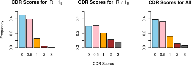
Figure 2: The CDR score distributions for the complete cases, the individuals missing at least one outcome variable, and the entire data set are provided in the left, middle, and right panels, respectively.

In Figure 2, we plot the CDR distribution for the complete cases, the individuals missing at least one outcome variable, and the entire data set, respectively. If the data was missing completely at random, we would expect the CDR score distribution to be mostly constant across all missing patterns of the data. However, we observe that for the complete cases, the dementia group (CDR score of 1, 2, or 3) makes up less than 20%, but the dementia group is close to 40% of the data that has at least one missing outcome variable. This suggests that the dementia group is severely underrepresented when we only perform analysis on the complete cases. Thus, from the plots, we can visually postulate the MCAR assumption to be unreasonable.

We select the model using prior knowledge. Since the CDR score has five levels, we also choose the same number. A similar number of groups will help with interpretability, and five is small enough that the number of parameters is manageable.

6.2 Point estimates and confidence intervals

In Table 1, we report the point estimates of the test score means and the corresponding standard errors in parentheses. There are a few takeaways. As reported, Classes 1 and 5 can be interpreted as the most and least healthy individuals, respectively. Note that in 6 out of 8 tests (omitting TRAIL A and TRAIL B), a higher score corresponds to better performance. On the other hand, TRAIL A and TRAIL B are scored using time-to-completion in seconds, so a higher score corresponds to a worse performance. For every test aside from TRAIL B, we observe a clear monotonic behavior in the test score means from Class 1 to Class 5, which suggests that the model is reasonable and fairly interpretable. For TRAIL B, Classes 4 and 5 have very similar mean test scores that are close to the maximum possible test score of 300. Since a test score of 300 indicates that the individual timed out and did not complete the test, this suggests that individuals from Classes 4 and 5 have comparable performance on the TRAIL B test.

Additionally, the results also suggests the different tests may have value at distinguishing individuals from different latent cognitive classes. For example, TRAIL A and TRAIL B are routinely used to measure executive function. Classes 4 and 5 represent the most unhealthy individuals in the population, but individuals in both perform similarly on TRAIL B. On the other hand, the mean test scores in Classes 4 and 5 for TRAIL A are very different, which suggests that TRAIL A can be a good discriminator between very unhealthy and moderately unhealthy individuals. As TRAIL B is a more complex task than TRAIL A, this seems to agree with our intuition.

Table 1: These tables contain point estimates of the test score means for each latent class. In the title of each column, we report the maximum possible score for a given test in parentheses. In each cell, the standard errors are reported in parentheses.

		Outcome Variables
		MMSE (30)	LOGIMEM (25)	MEMUNITS (25)	DIGIF (12)
Class	1	28.9 (0.01)	13.4 (0.04)	12.0 (0.05)	8.8 (0.02)
	2	26.8 (0.03)	9.1 (0.05)	7.1 (0.06)	7.7 (0.02)
	3	25.3 (0.06)	7.6 (0.08)	5.5 (0.08)	7.1 (0.03)
	4	22.5 (0.06)	5.3 (0.05)	3.5 (0.05)	6.6 (0.03)
	5	14.4 (0.12)	3.1 (0.05)	1.8 (0.04)	5.3 (0.04)

		DIGIB (12)	ANIMALS (77)	TRAILA (150)	TRAILB (300)
Class	1	7.2 (0.05)	20.9 (0.05)	28.4 (0.09)	65.9 (0.2)
	2	5.7 (0.02)	15.9 (0.05)	44.2 (0.17)	117.9 (0.43)
	3	4.9 (0.03)	13.5 (0.07)	57.2 (0.39)	209.7 (0.84)
	4	4.2 (0.02)	11.0 (0.06)	66.7 (0.36)	298.5 (0.08)
	5	2.7 (0.03)	6.9 (0.07)	145.3 (0.20)	295.2 (0.09)

In Table 2, we report the point estimates of the coefficients in the logistic regressions. One initial observation is that the coefficients of Age and Education are all positive and negative at the $\alpha=0.05$ significance level, respectively, across all classes. This implies that increasing age is associated with lower cognitive ability and higher education may provide some protection against dementia. The latter is known as the cognitive reserve hypothesis in the context of education (Meng and D’Arcy, 2012; Thow et al., 2018).

Table 2: This table contains point estimates for the coefficients for each of the covariates and each latent class. In each cell, the standard errors are reported in parentheses.

		Covariates
		Age	Education	Race	Sex
Class	2	0.06 (0.001)	-0.62 (0.028)	-0.37 (0.026)	0.72 (0.037)
	3	0.07 (0.002)	-0.9 (0.039)	0.45 (0.034)	0.93 (0.043)
	4	0.06 (0.002)	-1.06 (0.035)	0.36 (0.032)	0.79 (0.04)
	5	0.05 (0.002)	-1.14 (0.0041)	0.41 (0.0035)	0.93 (0.0041)

We can compare the magnitudes of the coefficient of Education to the coefficient of Age. For example, in Class 2, we observe $0.62/0.06\approx 10$, and in Class 5, we observe $1.14/0.05\approx 23$. This suggests that having a college degree or higher education may be equivalent to being 10-20 years younger in terms of cognitive ability.

6.3 Latent classes and clustering

We report two clustering results using models fit on the complete cases (Figure 3) and the entire data (Figure 4). For each set of clustering results, we visualize the clusters by plotting the CDR score composition of each of the five clusters. Furthermore, we report the mean of the CDR scores for each group, which gives a rough estimate on the group-specific clinical cognitive ability. From the complete case results (CC) in Figure 3, we generally see that the first clusters are primarily composed of healthy individuals as individuals with CDR scores of 0 take up larger proportions of the pie. As we progress to the middle latent classes, healthier individuals take up fewer proportion and individuals with mild cognitive impairment (CDR score of 0.5) take up larger proportion of the pie. Then, in Group 5, the majority of the individuals have some form of dementia.

For the clustering that used the entire data with the missing at random assumption (Figure 4), we observe a similar trend with the healthier individuals, the MCI individuals, and the dementia individuals being the dominant proportion in the earlier, middle, and later latent classes. However, the results from clustering the entire data set are more stark. In contrast with the complete clustering, Groups 4 and 5 contain a significantly higher number of individuals. Moreover, our model is able to detect a group of individuals with high dementia, as evidenced by Group 5’s mean CDR score of 1.55. Unlike the complete case clustering, Group 5 has almost 75% of individuals with some form of dementia. Many of these individuals would be omitted from the analysis if the missing data was not accounted for. Thus, accounting for the missingness leads to a clustering result with a stronger correlation with clinical assessments (CDR score).

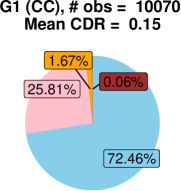
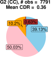
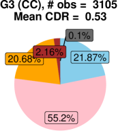
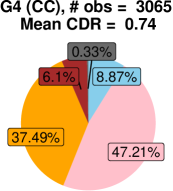
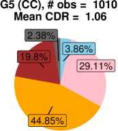
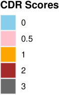
Figure 3: Clustering on complete data only. These pie charts summarize the composition of each of the five latent groups. We order the groups from most healthy to least healthy. This is reflected in the mean CDR score of each group.

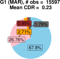
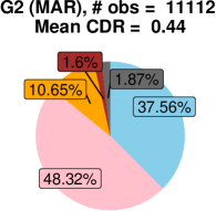
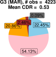
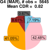
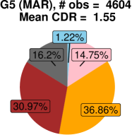
Figure 4: Clustering on the entire data with MAR assumption. These pie charts summarize the composition of each of the five latent groups. We order the groups from most healthy to least healthy. This is reflected in the mean CDR score of each group.

6.4 Incorporating longitudinal structure

Because the NACC data has individuals with repeated outcomes measurements over multiple years, we can track the predicted latent class over time for each individual. We call the latent class over time a latent trajectory. In the context of Alzheimer’s disease data, this can be used to observe an individual’s latent cognitive ability over time.

6.4.1 Latent class trajectory recovery

The process starts by obtaining a fitted model fit on the data consisting of the baseline covariates and the outcome variables measured on each individual’s initial entry into the study. For a constructive example, consider an individual $i$ with baseline covariates $\textbf{X}_{i}$ and $L$ repeated outcome measurements. For $\ell=1,\ldots,L$, let $\textbf{Y}_{i,\ell}$ and $\textbf{R}_{i,\ell}$ denote the outcome data and the missing pattern for the $i$th individual and $\ell$th time point, respectively. Note that we distinguish this from previous notations $Y_{i,j}$ and $R_{i,j}$ by using boldface to emphasize that these are vectors. Furthermore, let $\textbf{Y}_{i,\ell,\textbf{R}_{i,\ell}}$ denote the observed outcome variables for individual $i$ at time point $\ell$. We can compute $\hat{\pi}_{k,\textbf{R}_{i,\ell}}(\textbf{X}_{i},\textbf{Y}_{i,\ell,\textbf{R}_{i,\ell}})$ for every $i$ and $\ell$ using the fitted model. We can use these probabilities to cluster each individual at each time point, from which a latent trajectory can be constructed.

From the fitted model $p(\textbf{y}|\textbf{x};\bm{\theta},\bm{\beta})$, we assign each individual to a given cluster for each time point. In Figure 5, we provide an example of several latent trajectories over a span of five years. The $y$-axis denotes the latent class and the $x$-axis is the number of years since entry into the study; year $0$ corresponds to the year that the individual entered the study. For each data point at each time, we also report the CDR score.

For these individuals, we can observe that the latent trajectories depict a gradual change in cognitive ability. The trajectories are generally upward and to the right, which represent a general cognitive decline as the individuals are clustered in the more unhealthy classes as time progresses. Additionally, we can see that although the CDR score can be a useful summary for an individual, it may be insufficient to capture some aspects of one’s cognitive ability. Our model suggests that while CDR score may stay constant or may not shift much over time, there can be more change in the latent cognitive ability than one might expect. Thus, the latent classes predicted by our model may add an additional perspective because the CDR score is not assigned using knowledge of the neuropsychological test scores.

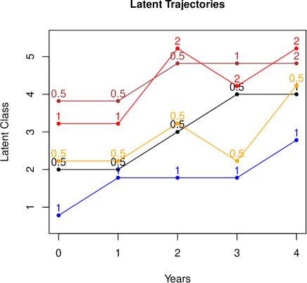
Figure 5: This figure depicts a spaghetti plot of multiple latent trajectories. Each trajectory denotes the latent class label of one individual over 4 years. We also label each point with the CDR score for each individual at a given time.

7 Discussion

In this paper, we have proposed a mixture of binomial experts model for modeling neuropsychological test score data. This model builds on classical ideas from the latent variable and mixture of experts literature. Through this model, we are able to construct a latent representation of an individual’s cognitive ability using their test scores and relate it to baseline covariates. Because the Alzheimer’s disease data set is both enriched with multivariate information and plagued with missing data, we address both of these issues. For each individual, we are able to perform clustering and generate a latent trajectory, a path of their cognitive ability in the latent space over time. We also provide analysis on the data on an aggregated level using transition matrices in Appendix G. Simulations are included in Appendix D. We outline how to perform estimation and inference under the MAR assumption.

There are several avenues for extending this paper. Our presented model has two key components: the weights $w_{k}(x;\beta_{k})$ and the component probabilities $p_{k}(y;\theta_{k})$. Due to the local independence assumption, the component probabilities $p_{k}(y;\theta_{k})$ reduce to a product of marginal distributions, which is a binomial product in this paper. One straightforward way to generalize this work is modifying these two working models to other parametric families. In our setting, the outcome data is discrete and bounded because we have neuropsychological test scores. However, often, outcome data can come in a variety of different forms such continuous, discrete, and mixed, as well as bounded and unbounded. For instance, in continuous and count data, respectively, the Gaussian and Poisson distributions may be applicable. Access to individual question level data may allow us to leverage ideas from item response theory and the Rasch model (Rasch, 1960). Additionally, since we are working with longitudinal data, there may be a way to incorporate time in the model, so that model-based clustering can be performed on entire trajectories rather than individuals at given a time point. There has been previous work on mixture of experts models applied to time series and longitudinal data (Waterhouse, MacKay and Robinson, 1995; Huerta, Jiang and Tanner, 2003; Tang and Qu, 2016), and it would be interesting to extend these frameworks to a model for multivariate longitudinal discrete data. Model selection is also another avenue for future exploration as we selected our model using prior knowledge. We included comments on AIC and BIC in Appendix E.

The MAR assumption is fundamental to our analysis of the NACC data as well as the inference procedure (Algorithm 3), but it is not the only option. Missing not at random (MNAR) assumptions encompass a rich class of potentially plausible assumptions. It would be interesting to explore MNAR assumptions in the context of latent variable modeling using methods such as pattern graphs (Chen, 2022b; Cheng et al., 2022; Suen and Chen, 2021). Additionally, perturbing the MAR as a form a sensitivity analysis remains largely an open question. We note that departures from missing at random would likely result in a significant modification of the elegant estimation procedure outlined in the paper because the ignorability condition would no longer hold. Missing not random assumptions often require stronger modeling assumptions because the relationship between Y and R needs to be modeled directly. We leave this for future work.

From a computational perspective, there is also an open question on how to speed up the algorithm. In practice, we check the convergence of Algorithms 1 and 3 using a prespecified tolerance $\epsilon$. If the $L_{2}$ norm between the current estimate and the previous estimate of $(\bm{\beta},\bm{\theta})$ is less than $\epsilon$, we assume that the algorithm has converged. Choosing a small $\epsilon$ is ideal but not practical because it can take a long time for the algorithm to terminate. An adaptive sequence of $\epsilon$ rather than a constant $\epsilon$ may be more ideal because we spend more time in the later iterations than the earlier ones. The concept of adaptive tolerance levels have been explored in another setting in the approximate Bayesian computation literature (Del Moral, Doucet and Jasra, 2012; Simola et al., 2021).

Appendix A Detailed Derivation of the EM Algorithm Update Equations

There are two EM algorithms described in this paper. The inner EM algorithm (Algorithm 1) is used to estimate the mixture of binomial product experts model while the outer EM algorithm (Algorithm 3) is used to fit the aforementioned model under a missing at random assumption. When there is no missingness, Algorithm 3 reduces to Algorithm 1. We discuss the details of both algorithms and the multiple imputation algorithm in the following three subsections.

A.1 Latent Variable EM

The E-step is easily obtained by calculating the $Q_{\text{LC},n}$ function. Since the only variable that is not conditioned on is $Z$, this is simply equivalent to changing all of the indicator variables in $\ell_{\text{LC},n}$ to conditional probabilities on X and Y.

Thus, the $Q_{\text{LC},n}$ function writes as

$$Q_{\text{LC},n}(\bm{\beta},\bm{\theta}|\textbf{X}_{1:n},\textbf{Y}_{1:n};\hat{\bm{\beta}}^{(t)},\hat{\bm{\theta}}^{(t)})$$

$$:=\frac{1}{n}\sum_{i=1}^{n}\sum_{k=1}^{K}\hat{\pi}_{k}^{(t)}(\textbf{X}_{i},\textbf{Y}_{i})\log w_{k}(\textbf{X}_{i};\beta_{k})+\frac{1}{n}\sum_{i=1}^{n}\sum_{k=1}^{K}\hat{\pi}_{k}^{(t)}(\textbf{X}_{i},\textbf{Y}_{i})\log p_{k}(\textbf{Y}_{i};\theta_{k}),$$ (A.1)

where

$$\hat{\pi}_{k}^{(t)}(\textbf{X}_{i},\textbf{Y}_{i}):=P(Z=k|\textbf{X}_{i},\textbf{Y}_{i};\hat{\bm{\beta}}^{(t)},\hat{\bm{\theta}}^{(t)})=\frac{w_{k}(\textbf{X}_{i};\hat{\beta}_{k}^{(t)})p_{k}(\textbf{Y}_{i};\hat{\theta}_{k}^{(t)})}{\sum_{k^{\prime}=1}^{K}w_{k^{\prime}}(\textbf{X}_{i};\hat{\beta}_{k^{\prime}}^{(t)})p_{k^{\prime}}(\textbf{Y}_{i};\hat{\theta}_{k^{\prime}}^{(t)})}.$$

We now derive the update equations in the M-step. Note that we update $(\bm{\beta},\bm{\theta})$ via

$$(\hat{\bm{\beta}}^{(t+1)},\hat{\bm{\theta}}^{(t+1)})=\operatorname*{argmax}_{\bm{\beta},\bm{\theta}}Q_{\text{LC},n}(\bm{\beta},\bm{\theta}|\textbf{X}_{1:n},\textbf{Y}_{1:n};\hat{\bm{\beta}}^{(t)},\hat{\bm{\theta}}^{(t)}).$$

Taking a partial derivative of (A.1) with respect to $\theta_{k,j}$, we obtain

$$\frac{\partial}{\partial\theta_{k,j}}\frac{1}{n}\sum_{i=1}^{n}\hat{\pi}_{k}^{(t)}(\textbf{X}_{i},\textbf{Y}_{i})\log\left(\binom{N_{j}}{Y_{i,j}}\theta_{k,j}^{Y_{i,j}}(1-\theta_{k,j})^{N_{j}-Y_{i,j}}\right)$$

$$=\frac{\partial}{\partial\theta_{k,j}}\frac{1}{n}\sum_{i=1}^{n}\hat{\pi}_{k}^{(t)}(\textbf{X}_{i},\textbf{Y}_{i})\cdot(Y_{i,j}\log\theta_{k,j}+(N_{j}-Y_{i,j})\log(1-\theta_{k,j}))$$

$$=\frac{1}{n}\sum_{i=1}^{n}\hat{\pi}_{k}^{(t)}(\textbf{X}_{i},\textbf{Y}_{i})\cdot\left(\frac{Y_{i,j}}{\theta_{k,j}}-\frac{N_{j}-Y_{i,j}}{1-\theta_{k,j}}\right).$$

Setting this derivative equal to $0$ yields the desired update equation for $\bm{\theta}$

$$\hat{\theta}_{k,j}^{(t+1)}=\frac{\sum_{i=1}^{n}\hat{\pi}_{k}^{(t)}(\textbf{X}_{i},\textbf{Y}_{i})\cdot\frac{Y_{i,j}}{N_{j}}}{\sum_{i=1}^{n}\hat{\pi}_{k}^{(t)}(\textbf{X}_{i},\textbf{Y}_{i})}.$$

We now discuss the update procedure for $\bm{\beta}$. We see that

$$\frac{1}{n}\sum_{i=1}^{n}\sum_{k=1}^{K}\hat{\pi}_{k}^{(t)}(\textbf{X}_{i},\textbf{Y}_{i})\log p_{k}(\textbf{Y}_{i};\theta_{k})$$

is the log-likelihood function with weights $\hat{\pi}_{k}^{(t)}(\textbf{X}_{i},\textbf{Y}_{i})$ rather than $1(Z_{i}=k)$, so we can apply a standard package that fits a logistic regression model using gradient ascent. However, instead of treating the dependent variable as $(1(Z_{i}=1),1(Z_{i}=2),\ldots,1(Z_{i}=K))$, we use the dependent variable $\mathbf{W}_{i}(\textbf{X}_{i},\textbf{Y}_{i})\equiv(\hat{\pi}_{1}^{(t)}(\textbf{X}_{i},\textbf{Y}_{i}),\hat{\pi}_{2}^{(t)}(\textbf{X}_{i},\textbf{Y}_{i}),\ldots,\hat{\pi}_{K}^{(t)}(\textbf{X}_{i},\textbf{Y}_{i}))$.

This completes the derivation of Algorithm 1.

A.2 Multiple Imputation under Missing at Random

The missing at random property equivalently can be written as

$$P(\textbf{R}=r|x,y)=P(\textbf{R}=r|x,y_{r}) \iff p(x,y,r)=p(x,y_{r},r)\cdot p(y_{\bar{r}}|y_{r},x)$$

$$\iff p(y_{\bar{r}}|y_{r},x,r)=p(y_{\bar{r}}|y_{r},x)$$

for all $r\in\mathcal{R}$.

Therefore, the imputation distribution $p(y_{\bar{r}}|y_{r},x,r)\equiv p(y_{\bar{r}}|y_{r},x)$ is constructed using the global model $p(y|x)$ that is fit on all of the data regardless of the missing data pattern.

Algorithm 2 requires the estimation of the conditional distribution $p(y_{\bar{r}}|y_{r},x;\bm{\beta},\bm{\theta})$ for every $r\in\mathcal{R}$. In the following derivation of the imputation distribution, we drop the parameters and reference to the iteration $t$ for readability. For any $r\in\mathcal{R}$, we have

$$p(y_{\bar{r}}|y_{r},x) =\frac{p(y|x)}{p(y_{r}|x)}$$

$$=\frac{p(y|x)}{\sum_{y_{\bar{r}}}p(y|x)}$$

$$=\frac{\sum_{k=1}^{K}w_{k}(x)\prod_{j=1}^{d}p_{k,j}(y_{j})}{\sum_{y_{\bar{r}}}\sum_{k=1}^{K}w_{k}(x)\prod_{j=1}^{d}p_{k,j}(y_{j})}$$

$$=\frac{\sum_{k=1}^{K}w_{k}(x)\prod_{j=1}^{d}p_{k,j}(y_{j})}{\sum_{k=1}^{K}w_{k}(x)\sum_{y_{\bar{r}}}\prod_{j=1}^{d}p_{k,j}(y_{j})}$$

$$=\frac{\sum_{k=1}^{K}w_{k}(x)\prod_{j=1}^{d}p_{k,j}(y_{j})}{\sum_{k=1}^{K}w_{k}(x)\prod_{r}p_{k,j}(y_{j})}$$

$$=\sum_{k=1}^{K}\underbrace{\frac{w_{k}(x)\prod_{j\in r}p_{k,j}(y_{j})}{\sum_{k=1}^{K}w_{k}(x)\prod_{j\in r}p_{k,j}(y_{j})}}_{W_{k,r}(x,y_{r})}\prod_{j\in\bar{r}}p_{k,j}(y_{j})$$

$$=\sum_{k=1}^{K}W_{k,r}(x,y_{r})\prod_{j\in\bar{r}}p_{k,j}(y_{j}).$$

Therefore, with a little algebra and the local independence assumption, we can show that the conditional distribution (and imputation distribution) remains a (reweighted) mixture of binomial products distribution, whose computation is fairly straightforward.

A.3 Missing at Random EM

Standard maximum likelihood inference can be viewed as constructing an $M$-estimator that estimates the population MLE

$$(\bm{\beta}_{0},\bm{\theta}_{0})=\operatorname*{argmax}_{\bm{\beta},\bm{\theta}}\mathbb{E}[\log p(\textbf{Y}|\textbf{X};\bm{\beta},\bm{\theta})].$$

By the law of iterated expectation, observe that

$$\mathbb{E}[\log p(\textbf{Y}|\textbf{X};\bm{\beta},\bm{\theta})] =\sum_{r}\mathbb{E}[\mathbb{E}\log p(\textbf{Y}|\textbf{X};\bm{\beta},\bm{\theta})|\textbf{X},\textbf{Y}_{r},\textbf{R}=r]\cdot 1(\textbf{R}=r)]$$

$$\stackrel{{\scriptstyle\text{MAR}}}{{=}}\sum_{r}\mathbb{E}[\mathbb{E}\log p(\textbf{Y}|\textbf{X};\bm{\beta},\bm{\theta})|\textbf{X},\textbf{Y}_{r}]\cdot 1(\textbf{R}=r)].$$ (A.2)

$$=\mathbb{E}\left[\sum_{r\in\mathcal{R}}\mathbb{E}[\log p(\textbf{Y}|\textbf{X};\bm{\beta},\bm{\theta})|\textbf{X},\textbf{Y}_{r}]\cdot 1(\textbf{R}=r)\right].$$ (A.3)

By converting equation (A.2) to the sample form, we obtain

$$Q_{\text{FC},n}(\bm{\beta},\bm{\theta}|\textbf{X}_{1:n},\textbf{Y}_{1:n};\hat{\bm{\beta}}^{(t)},\hat{\bm{\theta}}^{(t)}) =\frac{1}{n}\sum_{i=1}^{n}\sum_{r\in\mathcal{R}}Q_{\text{FC},r}(\bm{\beta},\bm{\theta}|\textbf{X}_{i},\textbf{Y}_{i,r};\hat{\bm{\beta}}^{(t)},\hat{\bm{\theta}}^{(t)})\cdot 1(\textbf{R}_{i}=r),$$

$$=\frac{1}{n}\sum_{i=1}^{n}Q_{\text{FC},\textbf{R}_{i}}(\bm{\beta},\bm{\theta}|\textbf{X}_{i},\textbf{Y}_{i,\textbf{R}_{i}};\hat{\bm{\beta}}^{(t)},\hat{\bm{\theta}}^{(t)}),$$ (A.4)

where $Q_{\text{FC},r}(\bm{\beta},\bm{\theta}|\textbf{X},\textbf{Y}_{r};\hat{\bm{\beta}}^{(t)},\hat{\bm{\theta}}^{(t)})=\mathbb{E}[\log p(\textbf{Y}|\textbf{X})|\textbf{X},\textbf{Y}_{r};\hat{\bm{\beta}}^{(t)},\hat{\bm{\theta}}^{(t)}]$. By construction, we expect that $Q_{\text{FC},n}(\bm{\beta},\bm{\theta}|\textbf{X}_{1:n},\textbf{Y}_{1:n};\hat{\bm{\beta}}^{(t)},\hat{\bm{\theta}}^{(t)})$ has expectation equal to $\mathbb{E}[\log p(\textbf{Y}|\textbf{X};\bm{\beta},\bm{\theta})]$. Unfortunately, we are not able to compute (A.4) because we do not have an explicit closed form expression for $Q_{\text{FC},r}(\bm{\beta},\bm{\theta}|\textbf{X},\textbf{Y}_{r};\hat{\bm{\beta}}^{(t)},\hat{\bm{\theta}}^{(t)})$. Thankfully, we can approximate it stochastically. For large enough $M$, we expect

$$\frac{1}{M}\sum_{m=1}^{M}\log p(\tilde{\textbf{Y}}^{(m;t)}|\textbf{X};\hat{\bm{\beta}}^{(t)},\hat{\bm{\theta}}^{(t)})\approx Q_{\text{FC},r}(\bm{\beta},\bm{\theta}|\textbf{X},\textbf{Y}_{r};\hat{\bm{\beta}}^{(t)},\hat{\bm{\theta}}^{(t)}),$$

where $\tilde{\textbf{Y}}^{(m;t)}=(\textbf{Y}_{r},\textbf{Y}_{\bar{r}}^{(m;t)})$, and for each $m$, $\textbf{Y}_{\bar{r}}^{(m;t)}\stackrel{{\scriptstyle\text{iid}}}{{\sim}}p(y_{\bar{r}}|\textbf{Y}_{r},\textbf{X};\hat{\bm{\beta}}^{(t)},\hat{\bm{\theta}}^{(t)})$. Thus, to complete the E-step, we replace the sample version above with a stochastic approximation

$$Q_{\text{FC},n}^{(M)}(\bm{\beta},\bm{\theta}|\textbf{X}_{1:n},\textbf{Y}_{1:n};\hat{\bm{\beta}}^{(t)},\hat{\bm{\theta}}^{(t)}) =\frac{1}{M}\sum_{m=1}^{M}\frac{1}{n}\sum_{i=1}^{n}\log p(\tilde{\textbf{Y}}_{i}^{(m;t)}|\textbf{X}_{i};\hat{\bm{\beta}}^{(t)},\hat{\bm{\theta}}^{(t)}),$$

where $\tilde{\textbf{Y}}_{i}^{(m;t)}=(\textbf{Y}_{i,\textbf{R}_{i}},\tilde{\textbf{Y}}_{i,\bar{\textbf{R}}_{i}}^{(m;t)})$. To actually perform this stochastic approximation in practice, we simply multiply impute $M$ times and stack the imputed data sets together.

The M-step is equivalent to maximizing the latent incomplete likelihood on the stacked imputed data set $\tilde{D}_{t}=\{(\textbf{X}_{i},\tilde{\textbf{Y}}_{i}^{(m;t)})\}_{i=1,\ldots,n;\ m=1,\ldots,M}$. Namely, we have

$$(\hat{\bm{\beta}}^{(t+1)},\hat{\bm{\theta}}^{(t+1)})=\operatorname*{argmax}_{\bm{\beta},\bm{\theta}}\frac{1}{n}\sum_{(\textbf{X}_{i},\tilde{\textbf{Y}}_{i}^{(m;t)})\in\tilde{D}_{t}}\ell_{\text{LI}}(\textbf{X}_{i},\tilde{\textbf{Y}}_{i}^{(m;t)}).$$

We showed in Section 2 that this can be maximized via an EM algorithm (Algorithm 1). Thus, the M-step of the outer EM algorithm is performed by Algorithm 1. This completes the derivation of Algorithm 3.

Appendix B Identification Theory

We make some brief comments on the identifiability of our model. The standard definition of identifiability implies that the mapping from the parameter space to the space of all probability distributions is one-to-one. However, this may be too strong for many practical purposes. For example, even the common problem of label swapping violates this identifiability definition, so researchers often consider the idea of identifiability up to permutation of the parameters. We now consider the notion of generic identifiability, which relaxes the definition of identifiability even further. Generic identifiability means identifiability holds almost everywhere in the parameter space (Allman, Matias and Rhodes, 2009). More formally, this means that the mapping from the parameter space to the space of probability distributions may fail to be one-to-one only on a set of Lebesgue measure zero. In a practical sense, this means that any such model fit on a given data set is unlikely to be unidentifiable, and we consider this notion to be sufficient for our applied data setting.

We provide sufficient conditions for generic identifiability in our mixture of binomial product experts model.

Proposition B.1 (Sufficient conditions for generic identifiability).

Suppose the following conditions hold.

1. Each mixture is distinct such that $\theta_{k}\neq\theta_{k^{\prime}}$ when $k\neq k^{\prime}$.

2. The number of outcome variables $d$ and the number of mixtures $K$ satisfies the bound $d\geq 2\lceil\log_{1+\min_{j}N_{j}}K\rceil+1$.

3. The logistic regression model $w_{k}(x;\beta_{k})$ for all $k\in[K]$ is identifiable.

Then, the mixture of binomial product experts is generically identifiable up to permutation of the parameters.

We note that the sufficient conditions outlined in Proposition B.1 are fairly mild. When there are at least $d=3$ outcome variables and the outcome variables belong to a moderate range, then $K$ can be fairly large. Note that the bound in Assumption A2 is likely to be able to be relaxed even further because it was built off of a general latent class model, where each mixture is assumed to be a product of multinomials rather than binomials. A mixture of binomial products is a submodel within the mixture of multinomial products model. A similar bound is discussed in Allman, Matias and Rhodes (2009) when all of the outcome variables have the same dimension.

The sufficient conditions for the identifiability of mixtures of binomials in the one dimensional case has been examined in Teicher (1961). Identification of the logistic regression model can be shown using standard assumptions such as the existence of an invertible design matrix and lack of complete separation. More recently, Ouyang and Xu (2022) have established sufficient and necessary conditions for the identifiability of latent class models with covariates.

Appendix C Comments on Code Implementation

C.1 Numerical Stability

We use the logsumexp trick, which is commonly used for numerical stability (McElreath, 2020). We are often interested in calculating probabilities of the form

$$(p_{1},\ldots,p_{K}),$$

where $\sum_{k=1}^{K}p_{k}=1$. In our work, probabilities are often formed by the product of multiple terms in the range $[0,1]$. Naive implementations can result in underflow, so we work with log-probabilities. Additionally, consider the scenario where

$$p_{k}=\frac{\exp(t_{k})}{\sum_{k^{\prime}=1}^{K}\exp(t_{k^{\prime}})}.$$

Then, we have

$$p_{k}=\exp\left(t_{k}-\left[c+\log\sum_{k^{\prime}=1}^{K}\exp(t_{k^{\prime}}-c)\right]\right)$$

for any constant $c$. The form inside the brackets is known as the logsumexp trick. If we pick $c=\max_{k^{\prime}}t_{k^{\prime}}$, then we can avoid most numerical underflows since each $t_{k^{\prime}}$ is shifted.

C.2 Random Initializations

We randomly initialize $\bm{\beta}$ and $\bm{\theta}$ using draws from uniform distributions. The intercept of each $\beta_{k}$ is drawn from $U[-1,1]$ while each slope term is drawn from $U[-0.5,0.5]$. We draw each $\theta_{k,j}$ from $U[0.1,0.9]$, so that it is initialized away from the boundary. All draws are performed independently.

Appendix D Simulations

We now examine the performance of our method in finite samples using simulated data. Each of the simulation studies is evaluated using the mean-squared error $\text{MSE}_{\bm{\theta}}=\mathbb{E}[\lVert\hat{\bm{\theta}}-\bm{\theta}\rVert_{2}]$ and $\text{MSE}_{\bm{\beta}}=\mathbb{E}[\lVert\hat{\bm{\beta}}-\bm{\beta}\rVert_{2}]$. We estimate the mean-squared error by simulating $U=1000$ data sets in each scenario and average the $L_{2}$ norm of the error over all the data sets. The estimated MSEs are calculated as follows

$$\widehat{\text{MSE}}_{\bm{\beta}}=\frac{1}{U}\sum_{i=1}^{U}\sum_{k\neq 1}\lVert\hat{\beta}_{k}^{(i)}-\beta_{k}\rVert_{2},\quad\widehat{\text{MSE}}_{\bm{\theta}}=\frac{1}{U}\sum_{i=1}^{U}\sum_{k}\lVert\hat{\theta}_{k}^{(i)}-\theta_{k}\rVert_{2},$$ (D.1)

where the superscript $(i)$ denotes the estimated parameter of the $i$th generated data set. We also construct 95% confidence intervals for each parameter and report the coverage over all the $U=1000$ data sets. We have $p=2$ covariates, $d=4$ outcome variables, and $K=3$ mixtures. Note that $\eta=2$, $\eta=2.5$, and $\eta=\infty$ correspond to approximately 75%, 85%, and 100% complete cases.

The missingness mechanism is specified to be missing at random with a total of 5 distinct missing patterns. We vary the selection model $P(\textbf{R}=r|\textbf{X},\textbf{Y})$, using a sensitivity parameter $\eta\in[0,\infty)$. First, we generate a prototype selection model via a logistic regression. For example, for pattern $r$, we have

$$\log\frac{P(\textbf{R}=r|\textbf{X},\textbf{Y}_{r})}{P(\textbf{R}\neq r|\textbf{X},\textbf{Y}_{r})}=\gamma_{r,0}+\gamma_{r,1}^{\top}\cdot(\textbf{X},\textbf{Y}_{r}),$$

where $\gamma_{r,0}=\lambda_{r,0}-\eta$. We use $\eta$ to control the amount of missingness. As $\eta\to\infty$, we have no missingness because $P(\textbf{R}=r|\textbf{X},\textbf{Y}_{r})\to 0$ for all $r\neq 1_{d}$.

Table 3: The first row contains results for the estimation of $\bm{\theta}$. The second row contains results for the estimation of $\bm{\beta}$.

$\textbf{MSE}_{\bm{\theta}}(\times 100)$
	Sample Size
	$n=500$	$n=1000$	$n=2000$
$\eta=\infty$	0.203	0.099	0.05
$\eta=2.5$	0.192	0.093	0.047
$\eta=2$	0.203	0.104	0.054

Average Coverage of $\theta$s
	Sample Size
	$n=500$	$n=1000$	$n=2000$
$\eta=\infty$	0.946	0.948	0.950
$\eta=2.5$	0.943	0.943	0.945
$\eta=2$	0.939	0.939	0.932

$\textbf{MSE}_{\bm{\beta}}(\times 100)$
	Sample Size
	$n=500$	$n=1000$	$n=2000$
$\eta=\infty$	12.7	6.05	3.08
$\eta=2.5$	41.5	20.6	10.5
$\eta=2$	40.5	20.0	10.1

Average Coverage of $\beta$s
	Sample Size
	$n=500$	$n=1000$	$n=2000$
$\eta=\infty$	0.949	0.951	0.947
$\eta=2.5$	0.952	0.951	0.944
$\eta=2$	0.956	0.951	0.950

As we are in a parametric model setting, we expect the MSE to decrease at rate of $n^{-1}$. Indeed, in the first column of Table 3, for a given $\eta$, we observe that the estimated MSE decreases at a roughly linear rate as we increase the sample size. This demonstrates that the estimation procedures for both the no missing data (Algorithm 1) and missing data cases (Algorithm 3) are consistent. The MSE for $\bm{\beta}$ is higher when there is missingness than when there is no missingness, which suggests that the estimating $\bm{\beta}$ becomes more difficult.

In the second column of Table 3, we generally observe nominal coverage as well. There is slight undercoverage of $\bm{\theta}$ when $\eta=2$. We attribute this to the fact that we do not have a closed-form expression for the MLE and there are many approximations in the algorithms. For example, Algorithm 3 is a stochastic EM algorithm because it relies on a prespecified number of imputations $M$. Increasing the number of imputations will decrease the Monte Carlo error at the cost of computational time. Additionally, we check convergence of Algorithms 1 and 3 using a set tolerance of $\epsilon=10^{-4}$. It is possible that the gradient of the log-likelihood surface can be fairly small in the neighborhood of the true MLE, leading to early stopping of the algorithms and returning a near-solution but not the true MLE. For most of the cases, the coverage is close to nominal, which suggests that the bootstrap procedure and the choice of initializing it at the original estimate returned by Algorithm 3 works in practice.

D.1 Simulation Details

We describe the data generating process. For the first simulation result, we have $p=2$ covariates and $d=4$ outcome variables. The model is described as follows:

$$p(x)=N\left(\begin{bmatrix}2\\ 3\end{bmatrix},\begin{bmatrix}1&0.2\\ 0.2&1\end{bmatrix}\right),\quad p(y|x)=\sum_{k=1}^{3}w_{k}(x;\beta_{k})\prod_{j=1}^{4}\binom{N_{j}}{y_{j}}\theta_{k,j}^{y_{j}}(1-\theta_{k,j})^{N_{j}-y_{j}},$$

where $\beta_{1}=(0,0,0)$, $\beta_{2}=(-1.5,0.3,0.4)$, and $\beta_{3}=(-2,0.5,0.25)$. The parameters for the binomials are as follows

$$\bm{\theta}=\begin{bmatrix}\theta_{1}\\ \theta_{2}\\ \theta_{3}\end{bmatrix}=\begin{bmatrix}0.8&0.8&0.8&0.8\\ 0.5&0.5&0.5&0.5\\ 0.1&0.1&0.1&0.1\end{bmatrix}.$$

To generate data for the missing data simulations, we use the same generating process as above, but we specify a selection model $P(R=r|x,y)$ to make the missing data. For every missing data pattern $r\neq 1111$, we generate the probabilities $P(R=r|x,y)=P(R=r|x,y_{r})$ under the following scheme to ensure MAR holds. We have

$$\log\frac{P(R=0001|x,y)}{P(R\neq 0001|x,y)}=(-2-\eta)-0.25x_{1}+0.3x_{2}+0.15y_{4},$$

$$\log\frac{P(R=0110|x,y)}{P(R\neq 0110|x,y)}=(-1-\eta)+0.3x_{1}-0.7x_{2}-0.1y_{2}+0.15y_{3},$$

$$\log\frac{P(R=1010|x,y)}{P(R\neq 1010|x,y)}=(-2-\eta)+0.7x_{1}-0.4x_{2}+0.24y_{1}-0.15y_{3},$$

$$\log\frac{P(R=1110|x,y)}{P(R\neq 1110|x,y)}=(-1-\eta)+0.2x_{1}-0.15x_{2}+0.15y_{1}-0.14y_{2}+0.05y_{3},$$

$$P(R=1111)=1-\sum_{r\neq 1111}P(R=r|x,y).$$

Here we treat $\eta\in[0,\infty)$ as a a parameter that controls the amount of missingness. As $\eta\to\infty$, $P(R=r|x,y)\to 0$ for every $r\neq 1111$, thereby, leading towards $P(R=1111|x,y)\to 1$ and consequently, a data set with no missing outcome variables.

Appendix E Comments on Model Selection

E.1 Model selection

In a standard data analysis, one key question is choosing the number of mixture components. In the case of no prior knowledge, we recommend using information criteria for model selection. The Akaike information criterion (AIC) Akaike (1973) and the Bayesian information criterion (BIC) Schwarz (1978) are popular methods for choosing the number of mixture components. Each of these information criteria works by adding a penalty term to the observed log-likelihood, defined above in (3.3).

Let $\nu(K)$ be the number of free parameters of the mixture of binomial product experts model with $K$ mixtures. We showed earlier that $\nu(K)=K(p+d+1)-p-1$. As functions of $K$, the AIC and BIC write as

$$\quad\text{AIC}(K):=2\nu(K)-2\ell_{\text{obs},n},\quad\text{BIC}(K):=\nu(K)\log n-2\ell_{\text{obs},n},$$

respectively. One can choose the model that minimizes the AIC or BIC.

For a given simulated data set of size $n=500$ and $\eta=\infty,2$ (details in Appendix D), Figure 6 summarizes the AIC and BIC for varying values of $K$. Both AIC and BIC criteria select the correct number $K=3$, showing that they are reasonable approaches for model selection.

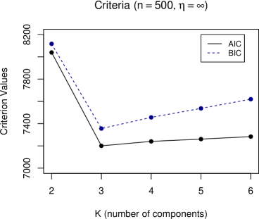
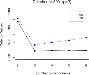
Figure 6: This figure depicts the AIC and BIC curves as we vary $K$ for a given simulated data set of size $n=500$ and $\eta=\infty,2$.

E.2 Model selection for the real data

The model is fit by treating the most healthy group as the baseline. For a given $K$, we fit the model with many random initializations and select the point estimate that maximizes the log-likelihood. For each $K$, we use the selected point estimate to compute AIC and BIC criteria. In Figure 7, we plot the AIC and BIC criteria as we vary the number of components in the mixture of binomial product experts model.

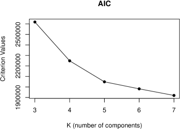
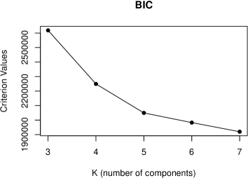
Figure 7: The left and right panels depict the AIC and BIC criteria as the number of components $K$ varies, respectively.

The choice based on prior knowledge of the CDR score (five levels, so $K=5$) coincides with the elbow location in both AIC and BIC curve (Tibshirani, Walther and Hastie, 2002). From the plot, we observe that the decrease in criteria values from $K=4$ to $K=5$ components is larger than subsequent decreases. Therefore, $K=5$ may also be viewed as a reasonable choice.

Appendix F Proofs

F.1 Nonconcavity of the Latent Incomplete Log-Likelihood (Lemma 2.1)

We demonstrate that a closed-form solution for the MLE of the mixture of binomial product experts model is unattainable due to the nonconcavity of the LI log-likelihood.

Proof of Lemma 2.1.

We consider a simple counterexample showing nonconcavity. Take $n=1$, $K=2$, $p=1$, and $d=3$. We further assume that $N_{1}=N_{2}=N_{3}=5$. This is the log-likelihood where there is exactly one data point with two clusters, a single covariate, and three bounded discrete outcome variables. Suppose that $\textbf{X}=1$ and $\textbf{Y}=(3,1,4)$. We have

$$\ell_{\text{LI},n}(\bm{\beta},\bm{\theta}|\textbf{X},\textbf{Y})=\log\left(\sum_{k=1}^{2}w_{k}(X;\beta_{k})\prod_{j=1}^{3}\binom{N_{j}}{y_{j}}\theta_{k,j}^{N_{j}}(1-\theta_{k,j})^{N_{j}-y_{j}}\right).$$

Consider two points $(\bm{\beta}^{1},\bm{\theta}^{1})$ and $(\bm{\beta}^{2},\bm{\theta}^{2})$, where the superscript indexes the data point. Let $\bm{\beta}^{1}=(-1,-1)$, $\bm{\theta}^{1}=(\theta_{1}^{1},\theta_{2}^{1})$, $\theta_{1}^{1}=(0.7,0.6,0.3)$, $\theta_{2}^{1}=(0.3,0.5,0.1)$, $\bm{\beta}^{2}=(1,6)$, $\bm{\theta}^{2}=(\theta_{1}^{2},\theta_{2}^{2})$, $\theta_{1}^{2}=(0.6,0.4,0.8)$, and $\theta_{2}^{2}=(0.4,0.3,0.3)$. We now consider the line that connects these two points and show that it sits above the function.

Observe that

$$\ell_{\text{LI},n}(t\bm{\beta}^{1}+(1-t)\bm{\beta}^{2},t\bm{\theta}^{1}+(1-t)\bm{\theta}^{2})\approx-6.81<-6.73\approx t\ell_{\text{LI},n}(\bm{\beta}^{1},\bm{\theta}^{1})+(1-t)\ell_{\text{LI},n}(\bm{\beta}^{2},\bm{\theta}^{2})$$

for $t=1/2$. Thus, nonconcavity is achieved.

∎

F.2 Identification Proposition (Proposition B.1)

Before we present the proof of this proposition, We first introduce a result from Allman, Matias and Rhodes (2009) on generic identification. Then, we state two helpful lemmas and providing their proofs.

Theorem F.1 (Theorem 4 of Allman, Matias and Rhodes (2009)).

Let $S_{1},\cdots,S_{d}$ be $d$ categorical variables and $S_{j}$ has $B_{j}$ categories. Consider a $K$-mixture model:

$$P(S=s;\lambda)=\prod_{k=1}^{K}\omega_{k}\prod_{j=1}^{d}q(s_{k,j};\lambda_{k,j}),$$

where $q(s_{k,j};\lambda_{k,j})$ is a multinomial distribution on the $B_{j}$ categories. Suppose there exists a partition $C_{1},C_{2},C_{3}$ of the set $\{1,2,\cdots,d\}$ such that $b_{j}=\prod_{j\in C_{j}}B_{j}$ and

$$\min\{d,b_{1}\}+\min\{d,b_{2}\}+\min\{d,b_{3}\}\geq 2K+2.$$

Then, the model $P(S=s;\lambda)$ is generically identifiable.

The first lemma describes the generic identifiability of the mixture of binomial products model without covariates.

Lemma F.2.

Consider the model

$$\sum_{k=1}^{K}w_{k}\left(\prod_{j=1}^{d}\binom{N_{j}}{y_{j}}(\theta_{k,j})^{y_{j}}(1-\theta_{k,j})^{N_{j}-y_{j}}\right).$$

If the dimension of the outcome variable $Y$ and the number of components satisfy $d\geq 2\lceil\log_{1+\min_{j}N_{j}}K\rceil+1$, then the model is generically identified up to permutation of the parameters.

Proof of Lemma F.2.

This result is a consequence of Theorem 4 from Allman, Matias and Rhodes (2009) (which is itself also a result following Kruskal’s theorem (Kruskal, 1976, 1977)), and the proof follows a similar construction provided in Corollary 5 from the same paper.

We argue that the latent class model with $K$ components and each $Y_{j}$ having dimension $N_{j}$ is generically identifiable under the aforementioned bound.

To simplify notation, let $M_{j}=1+N_{j}$ and $M_{*}=\min_{j}M_{j}$.

Let $K$ be fixed. First, consider the case that $d=2\lceil\log_{M_{*}}K\rceil+1$. Observe that

$${M_{*}}^{\lceil\log_{M_{*}}K\rceil-1}<K\leq{M_{*}}^{\lceil\log_{M_{*}}K\rceil}.$$

Partition the set $\{M_{j}\}_{j\in[d]}$ into a singleton $P_{3}=\{{M_{*}}\}$ and two sets $P_{1}$ and $P_{2}$ of equal size (each with cardinality $\lceil\log_{M_{*}}K\rceil$). Then, we have

$$\kappa_{1}:=\prod_{j\in P_{1}}M_{j}\geq M_{*}^{\lceil\log_{M_{*}}K\rceil},$$

$$\kappa_{2}:=\prod_{j\in P_{2}}M_{j}\geq M_{*}^{\lceil\log_{M_{*}}K\rceil},$$

$$\kappa_{3}:=\prod_{j\in P_{3}}M_{j}=M_{*}.$$

Then, it follows that $\min(K,\kappa_{1})=\min(K,\kappa_{2})=K$ and $\min(K,\kappa_{3})\geq 2$. Thus, we have

$$\min(K,\kappa_{1})+\min(K,\kappa_{2})+\min(K,\kappa_{3})\geq 2K+2.$$

When $d>2\lceil\log_{1+\min_{j}N_{j}}K\rceil+1$, one can partition $\{M_{j}\}_{j\in[d]}$ in a similar way such that $\kappa_{1}$ and $\kappa_{2}$ strictly increase. Therefore, the previous inequality will still hold.

Now, finally, note that a binomial model is a special case of a multinomial model and each $Y_{j}$ having dimension $N_{j}$. So binomial product models are special cases of the latent class model of multinomial in Theorem F.1. Generic identifiability of the larger model implies generic identifiability of the submodel. ∎

The following lemma is used to show how the generic identifiability of the “no covariates” model can imply the generic identifiability of the model with covariates under certain assumptions.

Lemma F.3.

Suppose the logistic regression model is identifiable, and each mixture is distinct. Then, the generic identifiability of the no covariate binomial product model implies the generic identifiability of the mixture of binomial product experts.

Proof of Lemma F.3.

As each mixture is distinct, this implies that the model

$$\sum_{k=1}^{K}w_{k}(x;\beta_{k})p_{k}(y;\theta_{k})$$

is constructed such that $\theta_{a}\neq\theta_{b}$ for $a\neq b$. We organize the parameters into one $\bm{\alpha}=(\bm{\beta},\bm{\theta})=(\beta_{1},\ldots,\beta_{K},\theta_{1},\ldots,\theta_{K})$ and $\alpha_{k}=(\beta_{k},\theta_{k})$. For $\sigma\in S_{K}$, where $S_{K}$ is the permutation group comprising all $K!$ mappings from $[K]$ to $[K]$, we use the notation $\bm{\beta}_{\sigma}$ and $\bm{\theta}_{\sigma}$ to denote the reordered tuples of $\bm{\beta}$ and $\bm{\theta}$, respectively, according to the permutation $\sigma$.

Now, consider a given covariate $x\in\mathcal{X}$, and suppose that

$$p(y|x;\bm{\alpha})=\sum_{k=1}^{K}w_{k}(x;\beta_{k})p_{k}(y;\theta_{k})=\sum_{k=1}^{K}w_{k}(x;\beta^{\prime}_{k})p_{k}(y;\theta^{\prime}_{k})=p(y|x;\bm{\alpha}^{\prime}).$$

By generic identification of the no covariate binomial product model up to permutation, we have

$$\bm{\theta}=\bm{\theta}^{\prime}_{\sigma_{x}}$$

for some permutation $\sigma_{x}\in S_{K}$. This permutation is indexed by $x$ because this permutation may depend on the covariate $x$.

We now argue that this permutation is the same for any $x$, thereby implying that the entire mixture of binomial products model is unique up to permutation. We proceed using a proof by contradiction. Let $x_{1}$ and $x_{2}$ be the covariates of two distinct observations with corresponding permutations $\sigma_{x_{1}}$ and $\sigma_{x_{2}}$ such that $\sigma_{x_{1}}\not\equiv\sigma_{x_{2}}$. Without loss of generality, assume that $\sigma_{x_{1}}$ is the identity permutation. So, for $x=x_{1}$, we have

$$\theta_{k}=\theta_{k}^{\prime}\quad\forall k\in[K]$$ (F.1)

by the identity permutation. For $x=x_{2}$, we have

$$\theta_{k}=\theta_{\sigma_{x_{2}}(k)}^{\prime}\quad\forall k\in[K].$$

Since $\sigma_{x_{2}}$ is not the identity permutation, there exists $g\in[K]$ such that $\sigma_{x_{2}}(g)\neq g$. Combining this fact with equation (F.1) via transitivity, we have

$$\theta_{g}^{\prime}=\theta_{g}=\theta_{\sigma_{x_{2}}(g)}^{\prime},$$

but this violates the distinct mixture assumption of $\theta_{a}\neq\theta_{b}$ for $a\neq b$. Thus, we have a contradiction, and the permutation $\sigma_{x}$ must be invariant to the covariate $x$. Finally, since the logistic regression model is identifiable, the mixture of binomial product experts model is generically identified up to permutation.

∎

We are now ready to present the proof of Proposition B.1 (this proves the generic identifiability of our mixture of binomial product experts model), which is a synthesis of results from the previous two lemmas.

Proof of Proposition B.1.

Since the inequality $d\geq 2\lceil\log_{1+\min_{j}N_{j}}K\rceil+1$ is satisfied by Assumption A2, we can invoke Lemma F.2. This implies that the model without covariates is generically identified.

Then, under Assumptions A1 and A3, we can invoke Lemma F.3. Thus, the model with covariates is also generically identified, thereby completing the proof. ∎

Appendix G More Real Data Analysis

G.1 Reproducibility of the Real Data Analysis

We report the distribution of the maximum log-likelihood estimates in Figure 8. We observe that most of the random initializations converge to a local maximum of the log-likelihood function, as evidenced by the mode of the distribution. This distribution indicates how important it is to have a sufficiently large number of random initializations in order to properly explore the parameter space. If the real data analysis was to repeated, we expect to obtain a similar histogram of log-likelihood values.

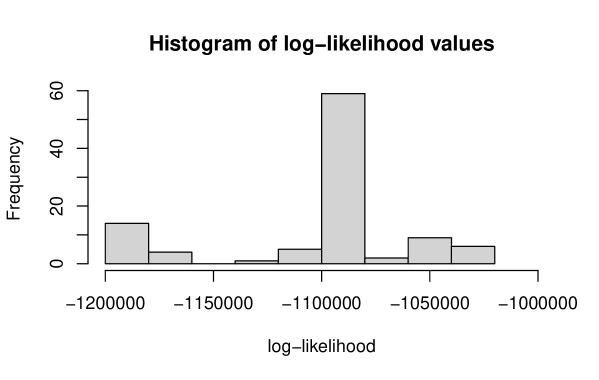
Figure 8: This figure is a histogram of the final log-likelihood values, reported over 100 random initializations, obtained using Algorithm 3 on the real data.

G.2 Transition matrix

Another quantity of interest is the transition in latent class after one year on an aggregated level rather than an individual level. To investigate this, we consider 21,604 individuals in which we have data when they entered the study and one year after. We predict the latent class at year 0 (time upon entering the study) and year 1 (one year after entering the study). Then, we can construct a transition matrix by computing the probability of falling into a given latent class at year 1 given that an individual was in a specific latent class at year 0.

Stratified by Age and Education, we have constructed a total of 10 transition matrices. The first set of transition matrices as reported in Table 4 is the transition matrix for all 21,604 individuals stratified by various age groups to observe the change in the transition matrix as individuals become older. Generally, we observe that most of the probabilities are concentrated along the diagonal, which suggests that after one year, individuals do not stray too far from the original predicted latent class on average. This also provides evidence to some stability of the clustering in the real data analysis. As individuals become older, we see that the transition matrices become increasingly upper triangular with fewer of the probability mass falling in the bottom right. This provides further evidence that older individuals are more likely to experience cognitive decline because they are more likely to fall into a more unhealthy class after one year. In particular, we can consider the cell in the first row and second column of each matrix stratified by age, indicating the transition from Latent Class 1 to Latent Class 2 in one year. For the seven age groups (younger than 65, 65-69, 70-74, 75-79, 80-84, 85-89, and older than 89), we observe the probabilities are 0.08, 0.12, 0.14, 0.19, 0.27, 0.27, and 0.37, respectively. This trend is monotonic and suggests that the cognitive decline is more severely pronounced for older individuals.

In Table 5, we stratify the data by lower and higher education (based on whether an individual has a college degree). We see that the higher education transition matrix appears to have more probability mass in the lower half than the lower education transition matrix. This suggests that in our data, individuals with a higher education are more likely to stay in the same latent class or progress to more healthy latent class after one year than individuals with lower education, providing further support for the cognitive reserve hypothesis and higher education.

Table 4: The following tables include the transition matrices for every individual in which we have their information after one year. We report the transition matrix for everyone in the top left and then stratify by age groups (younger than 65, 65-69, 70-74, 75-79, 80-84, 85-89, at least 90 years old) in the following matrices.

Total ($n=21604$)
		Year 1 Latent Class
		1	2	3	4	5
Year 0 Latent Class	1	0.83	0.14	0.01	0.01	0.00
	2	0.21	0.56	0.14	0.07	0.01
	3	0.05	0.28	0.30	0.31	0.07
	4	0.05	0.09	0.11	0.49	0.26
	5	0.12	0.06	0.02	0.09	0.72

Age $\bm{<}$ 65 ($n=4366$)
		Year 1 Latent Class
		1	2	3	4	5
Year 0 Latent Class	1	0.90	0.08	0.01	0.01	0.01
	2	0.30	0.44	0.13	0.10	0.03
	3	0.10	0.25	0.18	0.33	0.13
	4	0.10	0.06	0.06	0.41	0.36
	5	0.22	0.02	0.02	0.06	0.69

65 $\bm{\leq}$ Age $\bm{<}$ 70 ($n=3676$)
		Year 1 Latent Class
		1	2	3	4	5
Year 0 Latent Class	1	0.87	0.12	0.01	0.00	0.00
	2	0.27	0.51	0.14	0.07	0.01
	3	0.08	0.26	0.25	0.31	0.10
	4	0.06	0.09	0.10	0.43	0.32
	5	0.18	0.02	0.03	0.09	0.69

70 $\bm{\leq}$ Age $\bm{<}$ 75 ($n=4240$)
		Year 1 Latent Class
		1	2	3	4	5
Year 0 Latent Class	1	0.83	0.14	0.01	0.01	0.00
	2	0.24	0.55	0.12	0.07	0.01
	3	0.06	0.27	0.30	0.31	0.07
	4	0.05	0.11	0.11	0.47	0.26
	5	0.14	0.06	0.02	0.08	0.70

75 $\bm{\leq}$ Age $\bm{<}$ 80 ($n=4104$)
		Year 1 Latent Class
		1	2	3	4	5
Year 0 Latent Class	1	0.79	0.19	0.01	0.01	0.01
	2	0.20	0.59	0.14	0.07	0.01
	3	0.05	0.28	0.32	0.30	0.06
	4	0.03	0.07	0.15	0.53	0.22
	5	0.07	0.06	0.02	0.09	0.77

80 $\bm{\leq}$ Age $\bm{<}$ 85 ($n=3102$)
		Year 1 Latent Class
		1	2	3	4	5
Year 0 Latent Class	1	0.70	0.27	0.02	0.01	0.00
	2	0.15	0.63	0.15	0.06	0.01
	3	0.03	0.27	0.32	0.32	0.05
	4	0.02	0.12	0.12	0.51	0.23
	5	0.04	0.11	0.01	0.11	0.73

85 $\bm{\leq}$ Age $\bm{<}$ 90 ($n=1519$)
		Year 1 Latent Class
		1	2	3	4	5
Year 0 Latent Class	1	0.69	0.27	0.02	0.01	0.00
	2	0.12	0.62	0.18	0.07	0.02
	3	0.02	0.31	0.32	0.31	0.05
	4	0.00	0.10	0.13	0.56	0.21
	5	0.00	0.14	0.02	0.11	0.73

Age $\bm{\geq}$ 90 ($n=597$)
		Year 1 Latent Class
		1	2	3	4	5
Year 0 Latent Class	1	0.58	0.37	0.05	0.00	0.00
	2	0.10	0.56	0.20	0.11	0.03
	3	0.02	0.30	0.37	0.26	0.06
	4	0.00	0.13	0.08	0.55	0.24
	5	0.00	0.13	0.03	0.08	0.76

Table 5: We stratify the data by lower and higher education (based on whether an individual has a college degree). We report the results for lower education and higher education groups on the left and right, respectively.

Lower Education ($n=9114$)
		Year 1 Latent Class
		1	2	3	4	5
Year 0 Latent Class	1	0.78	0.19	0.02	0.01	0.01
	2	0.18	0.58	0.15	0.08	0.02
	3	0.03	0.27	0.33	0.32	0.05
	4	0.03	0.10	0.13	0.52	0.23
	5	0.07	0.08	0.02	0.10	0.73

Higher Education ($n=12490$)
		Year 1 Latent Class
		1	2	3	4	5
Year 0 Latent Class	1	0.85	0.13	0.01	0.01	0.00
	2	0.24	0.55	0.13	0.07	0.01
	3	0.07	0.28	0.26	0.30	0.09
	4	0.07	0.08	0.09	0.44	0.32
	5	0.18	0.03	0.02	0.08	0.69

DS was supported by NSF DGE-2140004. YC was supported by NSF DMS-195278, NSF DMS-2112907, NSF DMS-2141808, and NIH U24-AG072122.

References

- Akaike (1973) {binproceedings}[author] \bauthor\bsnmAkaike, \bfnmHirotugu\binitsH. (\byear1973). \btitleInformation theory and an extension of the maximum likelihood principle. In \bbooktitleSecond International Symposium on Information Theory (\beditor\bfnmBoris N\binitsB. N. \bsnmPetrov and \beditor\bfnmBela F\binitsB. F. \bsnmCsaki, eds.) \bpages267–281. \bpublisherAcademiai Kiado. \endbibitem
- Alashwal et al. (2019) {barticle}[author] \bauthor\bsnmAlashwal, \bfnmH\binitsH., \bauthor\bsnmEl Halaby, \bfnmM\binitsM., \bauthor\bsnmCrouse, \bfnmJJ\binitsJ., \bauthor\bsnmAbdalla, \bfnmA\binitsA. and \bauthor\bsnmMoustafa, \bfnmAA\binitsA. (\byear2019). \btitleThe Application of Unsupervised Clustering Methods to Alzheimer’s Disease. \bjournalFrontiers in Computational Neuroscience \bvolume13 \bpages31. \endbibitem
- Allman, Matias and Rhodes (2009) {barticle}[author] \bauthor\bsnmAllman, \bfnmElizabeth S.\binitsE. S., \bauthor\bsnmMatias, \bfnmCatherine\binitsC. and \bauthor\bsnmRhodes, \bfnmJohn A.\binitsJ. A. (\byear2009). \btitleIdentifiability of parameters in latent structure models with many observed variables. \bjournalThe Annals of Statistics \bvolume37 \bpages3099 – 3132. \endbibitem
- Anderson et al. (2019) {barticle}[author] \bauthor\bsnmAnderson, \bfnmMarti J.\binitsM. J., \bauthor\bparticlede \bsnmValpine, \bfnmPerry\binitsP., \bauthor\bsnmPunnett, \bfnmAndrew\binitsA. and \bauthor\bsnmMiller, \bfnmArden E.\binitsA. E. (\byear2019). \btitleA pathway for multivariate analysis of ecological communities using copulas. \bjournalEcology and Evolution \bvolume9 \bpages3276-3294. \endbibitem
- Bishop and Svenskn (2002) {binproceedings}[author] \bauthor\bsnmBishop, \bfnmChristopher M.\binitsC. M. and \bauthor\bsnmSvenskn, \bfnmMarkus\binitsM. (\byear2002). \btitleBayesian Hierarchical Mixtures of Experts. In \bbooktitleProceedings of the Nineteenth Conference on Uncertainty in Artificial Intelligence. \bseriesUAI’03 \bpages57–64. \bpublisherMorgan Kaufmann Publishers Inc., \baddressSan Francisco, CA, USA. \endbibitem
- Bock (1994) {binbook}[author] \bauthor\bsnmBock, \bfnmH. H.\binitsH. H. (\byear1994). \btitleInformation and Entropy in Cluster Analysis In \bbooktitleProceedings of the First US/Japan Conference on the Frontiers of Statistical Modeling: An Informational Approach: Volume 2 Multivariate Statistical Modeling \bpages115–147. \bpublisherSpringer Netherlands, \baddressDordrecht. \endbibitem
- Bouveyron et al. (2019) {bbook}[author] \bauthor\bsnmBouveyron, \bfnmCharles\binitsC., \bauthor\bsnmCeleux, \bfnmGilles\binitsG., \bauthor\bsnmMurphy, \bfnmT. Brendan\binitsT. B. and \bauthor\bsnmRaftery, \bfnmAdrian E.\binitsA. E. (\byear2019). \btitleModel-Based Clustering and Classification for Data Science: With Applications in R. \bseriesCambridge Series in Statistical and Probabilistic Mathematics. \bpublisherCambridge University Press. \endbibitem
- Boyle et al. (2018) {barticle}[author] \bauthor\bsnmBoyle, \bfnmPatricia A.\binitsP. A., \bauthor\bsnmYu, \bfnmLei\binitsL., \bauthor\bsnmWilson, \bfnmRobert S.\binitsR. S., \bauthor\bsnmLeurgans, \bfnmSue E.\binitsS. E., \bauthor\bsnmSchneider, \bfnmJulie A.\binitsJ. A. and \bauthor\bsnmBennett, \bfnmDavid A.\binitsD. A. (\byear2018). \btitlePerson-specific contribution of neuropathologies to cognitive loss in old age. \bjournalAnnals of Neurology \bvolume83 \bpages74-83. \endbibitem
- Brenowitz et al. (2017) {barticle}[author] \bauthor\bsnmBrenowitz, \bfnmWilla D\binitsW. D., \bauthor\bsnmHubbard, \bfnmRebecca A\binitsR. A., \bauthor\bsnmKeene, \bfnmC Dirk\binitsC. D., \bauthor\bsnmHawes, \bfnmStephen E\binitsS. E., \bauthor\bsnmLongstreth Jr, \bfnmWT\binitsW., \bauthor\bsnmWoltjer, \bfnmRandall L\binitsR. L. and \bauthor\bsnmKukull, \bfnmWalter A\binitsW. A. (\byear2017). \btitleMixed neuropathologies and estimated rates of clinical progression in a large autopsy sample. \bjournalAlzheimer’s & Dementia \bvolume13 \bpages654–662. \endbibitem
- Brintz, Fuentes and Madsen (2018) {barticle}[author] \bauthor\bsnmBrintz, \bfnmBen\binitsB., \bauthor\bsnmFuentes, \bfnmClaudio\binitsC. and \bauthor\bsnmMadsen, \bfnmLisa\binitsL. (\byear2018). \btitleAn asymptotic approximation to the N-mixture model for the estimation of disease prevalence. \bjournalBiometrics \bvolume74 \bpages1512-1518. \endbibitem
- Carreira-Perpinan and Renals (2000) {barticle}[author] \bauthor\bsnmCarreira-Perpinan, \bfnmMiguel A.\binitsM. A. and \bauthor\bsnmRenals, \bfnmSteve\binitsS. (\byear2000). \btitlePractical identifiability of finite mixtures of multivariate Bernoulli distributions. \bjournalNeural Computation \bvolume12 \bpages141–152. \endbibitem
- Chen (2022a) {barticle}[author] \bauthor\bsnmChen, \bfnmYen-Chi\binitsY.-C. (\byear2022a). \btitleStatistical Inference with Local Optima. \bjournalJournal of the American Statistical Association \bvolume0 \bpages1-13. \endbibitem
- Chen (2022b) {barticle}[author] \bauthor\bsnmChen, \bfnmYen-Chi\binitsY.-C. (\byear2022b). \btitlePattern graphs: A graphical approach to nonmonotone missing data. \bjournalThe Annals of Statistics \bvolume50 \bpages129 – 146. \endbibitem
- Chen et al. (2012) {barticle}[author] \bauthor\bsnmChen, \bfnmTao\binitsT., \bauthor\bsnmZhang, \bfnmNevin L.\binitsN. L., \bauthor\bsnmLiu, \bfnmTengfei\binitsT., \bauthor\bsnmPoon, \bfnmKin Man\binitsK. M. and \bauthor\bsnmWang, \bfnmYi\binitsY. (\byear2012). \btitleModel-based multidimensional clustering of categorical data. \bjournalArtificial Intelligence \bvolume176 \bpages2246-2269. \endbibitem
- Cheng et al. (2022) {barticle}[author] \bauthor\bsnmCheng, \bfnmGang\binitsG., \bauthor\bsnmChen, \bfnmYen-Chi\binitsY.-C., \bauthor\bsnmSmith, \bfnmMaureen A\binitsM. A. and \bauthor\bsnmZhao, \bfnmYing-Qi\binitsY.-Q. (\byear2022). \btitleHandling Nonmonotone Missing Data with Available Complete-Case Missing Value Assumption. \bjournalarXiv preprint arXiv:2207.02289. \endbibitem
- De Meyer et al. (2010) {barticle}[author] \bauthor\bsnmDe Meyer, \bfnmGeert\binitsG., \bauthor\bsnmShapiro, \bfnmFred\binitsF., \bauthor\bsnmVanderstichele, \bfnmHugo\binitsH., \bauthor\bsnmVanmechelen, \bfnmEugeen\binitsE., \bauthor\bsnmEngelborghs, \bfnmSebastiaan\binitsS., \bauthor\bsnmDe Deyn, \bfnmPeter Paul\binitsP. P., \bauthor\bsnmCoart, \bfnmEls\binitsE., \bauthor\bsnmHansson, \bfnmOskar\binitsO., \bauthor\bsnmMinthon, \bfnmLennart\binitsL., \bauthor\bsnmZetterberg, \bfnmHenrik\binitsH., \bauthor\bsnmBlennow, \bfnmKaj\binitsK., \bauthor\bsnmShaw, \bfnmLeslie\binitsL., \bauthor\bsnmTrojanowski, \bfnmJohn Q\binitsJ. Q. and \bauthor\bsnmInitiative, \bfnmAlzheimer’s Disease Neuroimaging\binitsA. D. N. (\byear2010). \btitleDiagnosis-Independent Alzheimer Disease Biomarker Signature in Cognitively Normal Elderly People. \bjournalArchives of Neurology \bvolume67 \bpages949-956. \endbibitem
- Del Moral, Doucet and Jasra (2012) {barticle}[author] \bauthor\bsnmDel Moral, \bfnmPierre\binitsP., \bauthor\bsnmDoucet, \bfnmArnaud\binitsA. and \bauthor\bsnmJasra, \bfnmAjay\binitsA. (\byear2012). \btitleAn adaptive sequential Monte Carlo method for approximate Bayesian computation. \bjournalStatistical Computing \bvolume22 \bpages1009–1020. \endbibitem
- Dempster, Laird and Rubin (1977) {barticle}[author] \bauthor\bsnmDempster, \bfnmA. P.\binitsA. P., \bauthor\bsnmLaird, \bfnmN. M.\binitsN. M. and \bauthor\bsnmRubin, \bfnmD. B.\binitsD. B. (\byear1977). \btitleMaximum Likelihood from Incomplete Data Via the EM Algorithm. \bjournalJournal of the Royal Statistical Society: Series B (Methodological) \bvolume39 \bpages1-22. \endbibitem
- Efron (1979) {barticle}[author] \bauthor\bsnmEfron, \bfnmBradley\binitsB. (\byear1979). \btitleBootstrap methods: Another look at the jackknife. \bjournalThe Annals of Statistics \bvolume7 \bpages1–26. \endbibitem
- Escudero, Zajicek and Ifeachor (2011) {binproceedings}[author] \bauthor\bsnmEscudero, \bfnmJavier\binitsJ., \bauthor\bsnmZajicek, \bfnmJohn P.\binitsJ. P. and \bauthor\bsnmIfeachor, \bfnmEmmanuel\binitsE. (\byear2011). \btitleEarly detection and characterization of Alzheimer’s disease in clinical scenarios using Bioprofile concepts and K-means. In \bbooktitle2011 Annual International Conference of the IEEE Engineering in Medicine and Biology Society \bpages6470-6473. \endbibitem
- Fruhwirth-Schnatter and Kaufmann (2008) {barticle}[author] \bauthor\bsnmFruhwirth-Schnatter, \bfnmSylvia\binitsS. and \bauthor\bsnmKaufmann, \bfnmSylvia\binitsS. (\byear2008). \btitleModel-Based Clustering of Multiple Time Series. \bjournalJournal of Business & Economic Statistics \bvolume26 \bpages78-89. \endbibitem
- Goodman (1974) {barticle}[author] \bauthor\bsnmGoodman, \bfnmLeo A.\binitsL. A. (\byear1974). \btitleExploratory Latent Structure Analysis Using Both Identifiable and Unidentifiable Models. \bjournalBiometrika \bvolume61 \bpages215–231. \endbibitem
- Gormley and Frühwirth-Schnatter (2018) {barticle}[author] \bauthor\bsnmGormley, \bfnmIsobel Claire\binitsI. C. and \bauthor\bsnmFrühwirth-Schnatter, \bfnmSylvia\binitsS. (\byear2018). \btitleHandbook of Mixture Analysis. \bjournalarXiv: Methodology. \endbibitem
- Gormley and Murphy (2008) {barticle}[author] \bauthor\bsnmGormley, \bfnmIsobel Claire\binitsI. C. and \bauthor\bsnmMurphy, \bfnmThomas Brendan\binitsT. B. (\byear2008). \btitleExploring Voting Blocs within the Irish Electorate: A Mixture Modeling Approach. \bjournalJournal of the American Statistical Association \bvolume103 \bpages1014–1027. \endbibitem
- Gu and Xu (2020) {barticle}[author] \bauthor\bsnmGu, \bfnmYuqi\binitsY. and \bauthor\bsnmXu, \bfnmGongjun\binitsG. (\byear2020). \btitlePartial identifiability of restricted latent class models. \bjournalThe Annals of Statistics \bvolume48 \bpages2082 – 2107. \endbibitem
- Gyllenberg et al. (1994) {barticle}[author] \bauthor\bsnmGyllenberg, \bfnmMats\binitsM., \bauthor\bsnmKoski, \bfnmTimo\binitsT., \bauthor\bsnmReilink, \bfnmEdwin\binitsE. and \bauthor\bsnmVerlaan, \bfnmMartin\binitsM. (\byear1994). \btitleNon-Uniqueness in Probabilistic Numerical Identification of Bacteria. \bjournalJournal of Applied Probability \bvolume31 \bpages542–548. \endbibitem
- Haines (2016) {barticle}[author] \bauthor\bsnmHaines, \bfnmLinda M.\binitsL. M. (\byear2016). \btitleMaximum likelihood estimation for N-mixture models. \bjournalBiometrics \bvolume72 \bpages1235-1245. \endbibitem
- Huang and Bandeen-Roche (2004) {barticle}[author] \bauthor\bsnmHuang, \bfnmGuan-Hua\binitsG.-H. and \bauthor\bsnmBandeen-Roche, \bfnmKaren\binitsK. (\byear2004). \btitleBuilding an identifiable latent class model with covariate effects on underlying and measured variables. \bjournalPsychometrika \bvolume69 \bpages5-32. \endbibitem
- Huerta, Jiang and Tanner (2003) {barticle}[author] \bauthor\bsnmHuerta, \bfnmGabriel\binitsG., \bauthor\bsnmJiang, \bfnmWenxin\binitsW. and \bauthor\bsnmTanner, \bfnmMartin A.\binitsM. A. (\byear2003). \btitleTIME SERIES MODELING VIA HIERARCHICAL MIXTURES. \bjournalStatistica Sinica \bvolume13 \bpages1097–1118. \endbibitem
- Jacobs et al. (1991) {barticle}[author] \bauthor\bsnmJacobs, \bfnmRobert A.\binitsR. A., \bauthor\bsnmJordan, \bfnmMichael I.\binitsM. I., \bauthor\bsnmNowlan, \bfnmSteven J.\binitsS. J. and \bauthor\bsnmHinton, \bfnmGeoffrey E.\binitsG. E. (\byear1991). \btitleAdaptive Mixtures of Local Experts. \bjournalNeural Computation \bvolume3 \bpages79–87. \endbibitem
- Jordan and Jacobs (1993) {binproceedings}[author] \bauthor\bsnmJordan, \bfnmM. I.\binitsM. I. and \bauthor\bsnmJacobs, \bfnmR. A.\binitsR. A. (\byear1993). \btitleHierarchical mixtures of experts and the EM algorithm. In \bbooktitleProceedings of 1993 International Conference on Neural Networks (IJCNN-93-Nagoya, Japan) \bvolume2 \bpages1339-1344 vol.2. \endbibitem
- Kang (2013) {barticle}[author] \bauthor\bsnmKang, \bfnmHyun\binitsH. (\byear2013). \btitleThe Prevention and Handling of Missing Data. \bjournalKorean Journal of Anesthesiology \bvolume64 \bpages402–406. \endbibitem
- Katzman et al. (1989) {barticle}[author] \bauthor\bsnmKatzman, \bfnmRobert\binitsR., \bauthor\bsnmAronson, \bfnmMurray\binitsM., \bauthor\bsnmFuld, \bfnmPaul\binitsP., \bauthor\bsnmKawas, \bfnmClaudia\binitsC., \bauthor\bsnmBrown, \bfnmTheodore\binitsT., \bauthor\bsnmMorgenstern, \bfnmHal\binitsH., \bauthor\bsnmFrishman, \bfnmWilliam\binitsW., \bauthor\bsnmGidez, \bfnmLarry\binitsL., \bauthor\bsnmEder, \bfnmHoward\binitsH. and \bauthor\bsnmOoi, \bfnmWee L\binitsW. L. (\byear1989). \btitleDevelopment of dementing illnesses in an 80-year-old volunteer cohort. \bjournalAnn Neurol \bvolume25 \bpages317-324. \endbibitem
- Kéry, Royle and Schmid (2005) {barticle}[author] \bauthor\bsnmKéry, \bfnmMarc\binitsM., \bauthor\bsnmRoyle, \bfnmJ. Andrew\binitsJ. A. and \bauthor\bsnmSchmid, \bfnmHans\binitsH. (\byear2005). \btitleModeling Avian Abundance from Replicated Counts Using Binomial Mixture Models. \bjournalEcological Applications \bvolume15 \bpages1450–1461. \endbibitem
- Kruskal (1976) {barticle}[author] \bauthor\bsnmKruskal, \bfnmJoseph B\binitsJ. B. (\byear1976). \btitleMore factors than subjects, tests and treatments: An indeterminacy theorem for canonical decomposition and individual differences scaling. \bjournalPsychometrika \bvolume41 \bpages281–293. \endbibitem
- Kruskal (1977) {barticle}[author] \bauthor\bsnmKruskal, \bfnmJoseph B\binitsJ. B. (\byear1977). \btitleThree-way arrays: Rank and uniqueness of trilinear decompositions, with application to arithmetic complexity and statistics. \bjournalLinear Algebra and its Applications \bvolume18 \bpages95–138. \endbibitem
- Lee and Harel (2022) {barticle}[author] \bauthor\bsnmLee, \bfnmJ. W.\binitsJ. W. and \bauthor\bsnmHarel, \bfnmO.\binitsO. (\byear2022). \btitleIncomplete Clustering Analysis via Multiple Imputation. \bjournalJournal of Applied Statistics \bvolume50 \bpages1962-1979. \endbibitem
- Levine and Casella (2001) {barticle}[author] \bauthor\bsnmLevine, \bfnmRichard A.\binitsR. A. and \bauthor\bsnmCasella, \bfnmGeorge\binitsG. (\byear2001). \btitleImplementations of the Monte Carlo EM Algorithm. \bjournalJournal of Computational and Graphical Statistics \bvolume10 \bpages422–439. \endbibitem
- Maslen et al. (2023) {barticle}[author] \bauthor\bsnmMaslen, \bfnmBen\binitsB., \bauthor\bsnmPopovic, \bfnmGordana\binitsG., \bauthor\bsnmLim, \bfnmMichelle\binitsM., \bauthor\bsnmMarzinelli, \bfnmEzequiel\binitsE. and \bauthor\bsnmWarton, \bfnmDavid\binitsD. (\byear2023). \btitleHow many sites? Methods to assist design decisions when collecting multivariate data in ecology. \bjournalMethods in Ecology and Evolution \bvolume14 \bpages1564-1573. \endbibitem
- Maydeu-Olivares and Liu (2015) {barticle}[author] \bauthor\bsnmMaydeu-Olivares, \bfnmAlbert\binitsA. and \bauthor\bsnmLiu, \bfnmYang\binitsY. (\byear2015). \btitleItem Diagnostics in Multivariate Discrete Data. \bjournalPsychological Methods \bvolume20 \bpages276–292. \endbibitem
- McElreath (2020) {bbook}[author] \bauthor\bsnmMcElreath, \bfnmRichard\binitsR. (\byear2020). \btitleStatistical Rethinking: A Bayesian Course with Examples in R and Stan, 2nd Edition, \bedition2 ed. \bpublisherCRC Press. \endbibitem
- McParland and Gormley (2013) {binproceedings}[author] \bauthor\bsnmMcParland, \bfnmDamien\binitsD. and \bauthor\bsnmGormley, \bfnmIsobel Claire\binitsI. C. (\byear2013). \btitleClustering Ordinal Data via Latent Variable Models. In \bbooktitleAlgorithms from and for Nature and Life (\beditor\bfnmBerthold\binitsB. \bsnmLausen, \beditor\bfnmDirk\binitsD. \bparticleVan den \bsnmPoel and \beditor\bfnmAlfred\binitsA. \bsnmUltsch, eds.) \bpages127–135. \bpublisherSpringer International Publishing, \baddressCham. \endbibitem
- Meng and D’Arcy (2012) {barticle}[author] \bauthor\bsnmMeng, \bfnmXiangfei\binitsX. and \bauthor\bsnmD’Arcy, \bfnmCarl\binitsC. (\byear2012). \btitleEducation and Dementia in the Context of the Cognitive Reserve Hypothesis: A Systematic Review with Meta-Analyses and Qualitative Analyses. \bjournalPLoS ONE \bvolume7. \endbibitem
- Mjørud et al. (2014) {barticle}[author] \bauthor\bsnmMjørud, \bfnmMarit\binitsM., \bauthor\bsnmRøsvik, \bfnmJanne\binitsJ., \bauthor\bsnmRokstad, \bfnmAnne Marie\binitsA. M., \bauthor\bsnmKirkevold, \bfnmMarit\binitsM. and \bauthor\bsnmEngedal, \bfnmKnut\binitsK. (\byear2014). \btitleVariables Associated with Change in Quality of Life Among Persons with Dementia in Nursing Homes: A 10 Months Follow-Up Study. \bjournalPLoS One \bvolume9 \bpagese115248. \endbibitem
- Ouyang and Xu (2022) {barticle}[author] \bauthor\bsnmOuyang, \bfnmJie\binitsJ. and \bauthor\bsnmXu, \bfnmGuofang\binitsG. (\byear2022). \btitleIdentifiability of Latent Class Models with Covariates. \bjournalPsychometrika \bvolume87 \bpages1343–1360. \endbibitem
- Qiu et al. (2019) {barticle}[author] \bauthor\bsnmQiu, \bfnmYing\binitsY., \bauthor\bsnmJacobs, \bfnmDawn M\binitsD. M., \bauthor\bsnmMesser, \bfnmKaren\binitsK., \bauthor\bsnmSalmon, \bfnmDavid P\binitsD. P. and \bauthor\bsnmFeldman, \bfnmHoward H\binitsH. H. (\byear2019). \btitleCognitive heterogeneity in probable Alzheimer disease: Clinical and neuropathologic features. \bjournalNeurology \bvolume93 \bpagese778-e790. \endbibitem
- Rasch (1960) {barticle}[author] \bauthor\bsnmRasch, \bfnmGeorg\binitsG. (\byear1960). \btitleProbabilistic models for some intelligence and attainment tests. \bjournalCopenhagen, Danish Institute for Educational Research. \endbibitem
- Robins and Wang (2000) {barticle}[author] \bauthor\bsnmRobins, \bfnmJames M.\binitsJ. M. and \bauthor\bsnmWang, \bfnmNaisyin\binitsN. (\byear2000). \btitleInference for Imputation Estimators. \bjournalBiometrika \bvolume87 \bpages113–124. \endbibitem
- Rost (1990) {barticle}[author] \bauthor\bsnmRost, \bfnmJürgen\binitsJ. (\byear1990). \btitleRasch Models in Latent Classes: An Integration of Two Approaches to Item Analysis. \bjournalApplied Psychological Measurement \bvolume14 \bpages271-282. \endbibitem
- Rubin (1976) {barticle}[author] \bauthor\bsnmRubin, \bfnmDonald B\binitsD. B. (\byear1976). \btitleInference and missing data. \bjournalBiometrika \bvolume63 \bpages581–592. \endbibitem
- Schwarz (1978) {barticle}[author] \bauthor\bsnmSchwarz, \bfnmGideon\binitsG. (\byear1978). \btitleEstimating the Dimension of a Model. \bjournalThe Annals of Statistics \bvolume6 \bpages461 – 464. \endbibitem
- Serafini, Murphy and Scrucca (2020) {bmisc}[author] \bauthor\bsnmSerafini, \bfnmAlessio\binitsA., \bauthor\bsnmMurphy, \bfnmThomas Brendan\binitsT. B. and \bauthor\bsnmScrucca, \bfnmLuca\binitsL. (\byear2020). \btitleHandling missing data in model-based clustering. \endbibitem
- Simola et al. (2021) {barticle}[author] \bauthor\bsnmSimola, \bfnmUmberto\binitsU., \bauthor\bsnmCisewski-Kehe, \bfnmJessi\binitsJ., \bauthor\bsnmGutmann, \bfnmMichael U.\binitsM. U. and \bauthor\bsnmCorander, \bfnmJukka\binitsJ. (\byear2021). \btitleAdaptive Approximate Bayesian Computation Tolerance Selection. \bjournalBayesian Analysis \bvolume16 \bpages397 – 423. \endbibitem
- Sportisse et al. (2023) {bmisc}[author] \bauthor\bsnmSportisse, \bfnmAude\binitsA., \bauthor\bsnmMarbac, \bfnmMatthieu\binitsM., \bauthor\bsnmBiernacki, \bfnmChristophe\binitsC., \bauthor\bsnmBoyer, \bfnmClaire\binitsC., \bauthor\bsnmCeleux, \bfnmGilles\binitsG., \bauthor\bsnmJosse, \bfnmJulie\binitsJ. and \bauthor\bsnmLaporte, \bfnmFabien\binitsF. (\byear2023). \btitleModel-based Clustering with Missing Not At Random Data. \endbibitem
- Stern (2012) {barticle}[author] \bauthor\bsnmStern, \bfnmYaakov\binitsY. (\byear2012). \btitleCognitive reserve in ageing and Alzheimer’s disease. \bjournalLancet Neurology \bvolume11 \bpages1006–1012. \endbibitem
- Suen and Chen (2021) {bmisc}[author] \bauthor\bsnmSuen, \bfnmDaniel\binitsD. and \bauthor\bsnmChen, \bfnmYen-Chi\binitsY.-C. (\byear2021). \btitleMultistage Estimators for Missing Covariates and Incomplete Outcomes. \endbibitem
- Tang and Qu (2016) {barticle}[author] \bauthor\bsnmTang, \bfnmXiwei\binitsX. and \bauthor\bsnmQu, \bfnmAnnie\binitsA. (\byear2016). \btitleMixture Modeling for Longitudinal Data. \bjournalJournal of Computational and Graphical Statistics \bvolume25 \bpages1117–1137. \endbibitem
- Teicher (1961) {barticle}[author] \bauthor\bsnmTeicher, \bfnmHenry\binitsH. (\byear1961). \btitleIdentifiability of Mixtures. \bjournalThe Annals of Mathematical Statistics \bvolume32 \bpages244 – 248. \endbibitem
- Thomas, Lohaus and Brainerd (1993) {barticle}[author] \bauthor\bsnmThomas, \bfnmHoben\binitsH., \bauthor\bsnmLohaus, \bfnmArnold\binitsA. and \bauthor\bsnmBrainerd, \bfnmC. J.\binitsC. J. (\byear1993). \btitleModeling Growth and Individual Differences in Spatial Tasks. \bjournalMonographs of the Society for Research in Child Development \bvolume58 \bpagesi–190. \endbibitem
- Thow et al. (2018) {barticle}[author] \bauthor\bsnmThow, \bfnmMegan E\binitsM. E., \bauthor\bsnmSummers, \bfnmMathew J\binitsM. J., \bauthor\bsnmSaunders, \bfnmNichole L\binitsN. L., \bauthor\bsnmSummers, \bfnmJeffery J\binitsJ. J., \bauthor\bsnmRitchie, \bfnmKaren\binitsK. and \bauthor\bsnmVickers, \bfnmJames C\binitsJ. C. (\byear2018). \btitleFurther education improves cognitive reserve and triggers improvement in selective cognitive functions in older adults: The Tasmanian Healthy Brain Project. \bjournalAlzheimer’s & dementia : diagnosis, assessment & disease monitoring \bvolume10 \bpages22-30. \endbibitem
- Tibshirani, Walther and Hastie (2002) {barticle}[author] \bauthor\bsnmTibshirani, \bfnmRobert\binitsR., \bauthor\bsnmWalther, \bfnmGuenther\binitsG. and \bauthor\bsnmHastie, \bfnmTrevor\binitsT. (\byear2002). \btitleEstimating the Number of Clusters in a Data Set Via the Gap Statistic. \bjournalJournal of the Royal Statistical Society Series B: Statistical Methodology \bvolume63 \bpages411-423. \endbibitem
- Tosto et al. (2016) {barticle}[author] \bauthor\bsnmTosto, \bfnmGiuseppe\binitsG., \bauthor\bsnmMonsell, \bfnmSarah E.\binitsS. E., \bauthor\bsnmHawes, \bfnmStephen E.\binitsS. E., \bauthor\bsnmBruno, \bfnmGiuseppe\binitsG. and \bauthor\bsnmMayeux, \bfnmRichard\binitsR. (\byear2016). \btitleProgression of Extrapyramidal Signs in Alzheimer’s Disease: Clinical and Neuropathological Correlates. \bjournalJournal of Alzheimer’s Disease \bvolume49 \bpages1085-1093. \endbibitem
- van Buuren and Groothuis-Oudshoorn (2011) {barticle}[author] \bauthor\bparticlevan \bsnmBuuren, \bfnmStef\binitsS. and \bauthor\bsnmGroothuis-Oudshoorn, \bfnmKarin\binitsK. (\byear2011). \btitlemice: Multivariate Imputation by Chained Equations in R. \bjournalJournal of Statistical Software \bvolume45 \bpages1–67. \endbibitem
- van der Vaart (1998) {bbook}[author] \bauthor\bparticlevan der \bsnmVaart, \bfnmAad W\binitsA. W. (\byear1998). \btitleAsymptotic statistics \bvolume3. \bpublisherCambridge university press. \endbibitem
- Vermunt (2010) {barticle}[author] \bauthor\bsnmVermunt, \bfnmJeroen K.\binitsJ. K. (\byear2010). \btitleLatent Class Modeling with Covariates: Two Improved Three-Step Approaches. \bjournalPolitical Analysis \bvolume18 \bpages450–469. \endbibitem
- Wang and Robins (1998) {barticle}[author] \bauthor\bsnmWang, \bfnmNaisyin\binitsN. and \bauthor\bsnmRobins, \bfnmJames M.\binitsJ. M. (\byear1998). \btitleLarge-Sample Theory for Parametric Multiple Imputation Procedures. \bjournalBiometrika \bvolume85 \bpages935–948. \endbibitem
- Waterhouse, MacKay and Robinson (1995) {binproceedings}[author] \bauthor\bsnmWaterhouse, \bfnmSteve\binitsS., \bauthor\bsnmMacKay, \bfnmDavid\binitsD. and \bauthor\bsnmRobinson, \bfnmAnthony\binitsA. (\byear1995). \btitleBayesian Methods for Mixtures of Experts. In \bbooktitleAdvances in Neural Information Processing Systems (\beditor\bfnmD.\binitsD. \bsnmTouretzky, \beditor\bfnmM. C.\binitsM. C. \bsnmMozer and \beditor\bfnmM.\binitsM. \bsnmHasselmo, eds.) \bvolume8. \bpublisherMIT Press. \endbibitem
- Yesavage et al. (2016) {barticle}[author] \bauthor\bsnmYesavage, \bfnmJerome A.\binitsJ. A., \bauthor\bsnmTaylor, \bfnmJoy L.\binitsJ. L., \bauthor\bsnmFriedman, \bfnmLee\binitsL., \bauthor\bsnmRosenberg, \bfnmPaul B.\binitsP. B., \bauthor\bsnmLazzeroni, \bfnmLaura C.\binitsL. C., \bauthor\bsnmLeoutsakos, \bfnmJeannie S.\binitsJ. S., \bauthor\bsnmKinoshita, \bfnmLisa M.\binitsL. M., \bauthor\bsnmPerlow, \bfnmMichael J.\binitsM. J., \bauthor\bsnmMunro, \bfnmCynthia A.\binitsC. A., \bauthor\bsnmDevanand, \bfnmD. P.\binitsD. P., \bauthor\bsnmDrye, \bfnmLea T.\binitsL. T., \bauthor\bsnmMintzer, \bfnmJacobo E.\binitsJ. E., \bauthor\bsnmPollock, \bfnmBruce G.\binitsB. G., \bauthor\bsnmPorsteinsson, \bfnmAnton P.\binitsA. P., \bauthor\bsnmSchneider, \bfnmLon S.\binitsL. S., \bauthor\bsnmShade, \bfnmDavid M.\binitsD. M., \bauthor\bsnmWeintraub, \bfnmDaniel\binitsD., \bauthor\bsnmLyketsos, \bfnmConstantine G.\binitsC. G., \bauthor\bsnmNoda, \bfnmAkihiko\binitsA. and \bauthor\bsnmGroup, \bfnmCitAD Research\binitsC. R. (\byear2016). \btitlePrincipal components analysis of agitation outcomes in Alzheimer’s disease. \bjournalJournal of Psychiatric Research \bvolume79 \bpages4–7. \endbibitem
- Yuksel, Wilson and Gader (2012) {barticle}[author] \bauthor\bsnmYuksel, \bfnmSeniha\binitsS., \bauthor\bsnmWilson, \bfnmJoseph\binitsJ. and \bauthor\bsnmGader, \bfnmPaul\binitsP. (\byear2012). \btitleTwenty Years of Mixture of Experts. \bjournalIEEE Transactions on Neural Networks and Learning Systems \bvolume23 \bpages1177-1193. \endbibitem
- Zhang (2004) {barticle}[author] \bauthor\bsnmZhang, \bfnmNevin L.\binitsN. L. (\byear2004). \btitleHierarchical Latent Class Models for Cluster Analysis. \bjournalJournal of Machine Learning Research \bvolume5 \bpages697–723. \endbibitem
- Zhang et al. (1990) {barticle}[author] \bauthor\bsnmZhang, \bfnmMingyuan\binitsM., \bauthor\bsnmKatzman, \bfnmRobert\binitsR., \bauthor\bsnmSalmon, \bfnmDavid\binitsD., \bauthor\bsnmJin, \bfnmHui\binitsH., \bauthor\bsnmCai, \bfnmGuangjie\binitsG., \bauthor\bsnmWang, \bfnmZhaoyu\binitsZ., \bauthor\bsnmQu, \bfnmGuoying\binitsG., \bauthor\bsnmGrant, \bfnmIgor\binitsI., \bauthor\bsnmYu, \bfnmEn\binitsE., \bauthor\bsnmLevy, \bfnmPhil\binitsP. \betalet al. (\byear1990). \btitleThe prevalence of dementia and Alzheimer’s disease in Shanghai, China: impact of age, gender, and education. \bjournalAnnals of Neurology \bvolume27 \bpages428–437. \endbibitem