A priori screening of data-enabled turbulence models

Abstract

Assessing the compliance of a white-box turbulence model with known turbulent knowledge is straightforward. It enables users to screen conventional turbulence models and identify apparent inadequacies, thereby allowing for a more focused and fruitful validation and verification. However, comparing a black-box machine-learning model to known empirical scalings is not straightforward. Unless one implements and tests the model, it would not be clear if a machine-learning model, trained at finite Reynolds numbers preserves the known high Reynolds number limit. This is inconvenient, particularly because model implementation involves retraining and re-interfacing. This work attempts to address this issue, allowing fast a priori screening of machine-learning models that are based on feed-forward neural networks (FNN). The method leverages the mathematical theorems we present in the paper. These theorems offer estimates of a network’s limits even when the exact weights and biases are unknown. For demonstration purposes, we screen existing machine-learning wall models and RANS models for their compliance with the log layer physics and the viscous layer physics in an a priori manner. In addition, the theorems serve as essential guidelines for future machine-learning models.

I Introduction

The range of scales in high Reynolds number turbulent flows spans multiple orders of magnitude. Conducting a direct numerical simulation (DNS) that resolves all these scales is prohibitively expensive at high Reynolds numbers li2022grid ; yang2021grid ; choi2012grid , leading to the need for turbulence modeling. Examples of turbulence modeling include sub-grid scale modeling and wall modeling in large-eddy simulation (LES) meneveau2000scale ; piomelli2002wall ; bose2018wall , as well as Reynolds stress modeling in Reynolds-averaged Navier-Stokes (RANS) durbin2018some . Conventional turbulence models (in particular, RANS models) rely heavily on empirical scalings, in addition to knowledge derived from first principles such as Galilean invariance and realizability. These empirical scalings include power-law decay of unforced isotropic turbulence thormann2014decay , the law of the wall (LoW) marusic2013logarithmic , Kolmogorov’s hypotheses of small-scale turbulence kolmogorov1941dissipation , as well as Townsend’s attached eddy hypothesis marusic2019attached ; yang2019hierarchical ; yang2018hierarchical ; duraisamy2023uncovering , among many others pope2000turbulent . While these empirical scalings are not derived from first principles, they have been extensively validated and are expected to hold even under unseen conditions. The most well-known example is probably the LoW. Although it cannot be derived directly from the Navier-Stokes equations, numerous studies have demonstrated its validity in canonical wall flows (pipe, channel, flat plate) with no bulk acceleration hutchins2009hot ; hultmark2012turbulent ; rosenberg2013turbulence ; lee2015direct ; hoyas2022wall ; xu2021flow . It is commonly believed that the log law remains valid at larger Reynolds numbers, potentially extending to infinity. Compliance with empiricisms like the log law serves as a straightforward criterion for assessing turbulence models. For instance, a model intended for wall-bounded flows but failing to preserve the law of the wall is deficient and should be discarded spalart2015philosophies . Being able to confidently screen out a model with critical flaws without having to implement/verify/validate it is not only prudent and robust from the physics point of view, but also efficient from a user’s perspective duraisamy2019turbulence ; pradhan2023unified : V&V campaigns for RANS models require considerable time and collective efforts rumsey2011summary ; rumsey2015overview ; rumsey2019overview ; tinoco2018summary .

A need for such simple criteria exists for data-based machine-learning models as well. In fact, with the increasing number of machine-learning models available singh2017machine ; tenney2020application ; yin2022iterative ; fang2023toward ; pan2018data ; wang2017physics ; zhao2020rans ; xie2021artificial ; xie2020modeling ; huang2019wall ; Vadrot2023 and the challenges associated with their implementations rumsey2022search ; vadrot2022survey , the ability to identify models that are lacking extrapolation of key flow physics is more valuable for machine-learning models than for conventional empirical models. However, assessing whether a machine-learning model adheres to known knowledge is not a straightforward task. Unlike conventional turbulence models that are white-box models, machine-learning models, except for a few exceptions weatheritt2017development ; zhao2020rans ; brunton2016discovering ; hansen2023data , are black-box ones. How to evaluate the asymptotic behavior of a black box in an a priori manner is not clear. Consider, for example, the machine-learning model in Ref. yang2019predictive . The model is a feedforward neural network. The network is trained against the $\rm Re_{\tau}=1000$ channel flow DNS in Ref. graham2016web . It takes the instantaneous $U^{+}/\ln(y^{+})$ and $y^{+}/U^{+}$ as its inputs and computes the instantaneous wall-shear stress $\tau^{+}_{w}$ as its output. It is not evident in an a priori sense whether this trained network would preserve the law of the wall. As a result, it is difficult to dismiss a machine-learning model without implementing, validating, and verifying it. This is undesirable, particularly considering that implementing a machine-learning model involves re-training and adapting it to different code environments. Furthermore, due to the lack of satisfactory results from machine-learning models in the field of computational fluid dynamics (CFD) rumsey2022search , the high labor cost associated with assessing these models hinders their widespread adoption in engineering practice.

The present work aims to tackle the aforementioned challenge. We focus on a priori examination of whether feedforward-neural-network-based (FNN-based) machine-learning models respect the LoW. While it is acknowledged that not all machine-learning models are based on FNNs bhatnagar2019prediction ; xu2020multi ; duvall2021discretization ; bakarji2022dimensionally ; liu2022new ; huang2023distilling ; xiang2021neuroevolution ; li2023long , a substantial number of them are. Examples include tensor-based neural networks ling2016reynolds , physics-informed machine learning xiao2020flows ; tao2020physics , field inversion and machine learning singh2017machine , progressive machine learning bin2022progressive ; bin2023data , among others. Regarding the LoW, although there is other known knowledge that is fundamental to turbulence models, the LoW is regarded by many to be the most important one menter2019best ; spalart2015philosophies . The remainder of the paper is organized as follows. We present the technical background and the mathematical theorems in section II. In section III, we apply the theorems to assess the existing machine-learning models in the literature. Finally, we conclude in section IV.

II Background and theorems

This section is organized as follows. An overview of FNN is given in section II.1. In section II.2, we present four mathematical theorems which form the foundation of the present work. Their proofs are presented in the Appendix. Lastly, we summarize the physical scalings in section II.3.

II.1 Feedforward neural networks

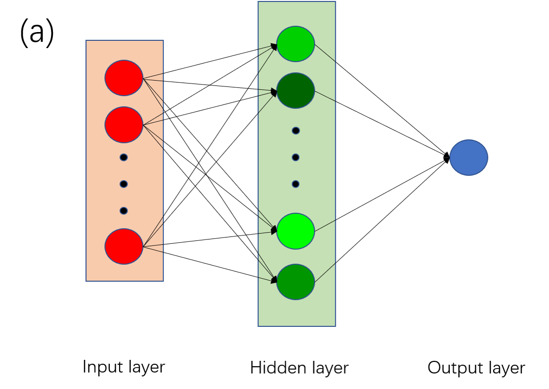
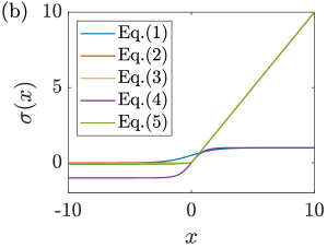
Figure 1: (a) A schematic of an FNN. The shade of the color represents the value of the activation function. (b) Some activation functions.

Figure 1(a) shows a schematic of a feedforward neural network (FNN). The FNN contains an input layer, a hidden layer, and an output layer. A general FNN maps $\mathbb{R}^{N}$ to $\mathbb{R}^{M}$, where $N$ and $M$ are the dimensions of the input and the output space. Such an FNN can, however, be split into $M$ FNNs whose output is strictly one-dimensional. Without loss of generality, we focus on the case where $M=1$.

The neurons in the hidden layer receive input signals from the previous layer, compute outputs, and send the output signals to the next layer. The commonly employed activation functions include the sigmoid function, the ReLU function, the leaky-ReLU function, the tanh-sigmoid function, and the exponential linear unit function, which are ploted in figure 1(b) and are shown below. The sigmoid function reads

$$\sigma(x)=\frac{1}{1+e^{-x}}.$$ (1)

The ReLU function reads

$$\sigma(x)=\begin{cases}x&x\geq 0\\ 0&x<0\end{cases}.$$ (2)

The leaky-ReLU function reads

$$\sigma(x)=\begin{cases}x&x\geq 0\\ \gamma x&x<0\end{cases},$$ (3)

where $\gamma$ is a parameter. The tanh-sigmoid function reads

$$\sigma(x)=\frac{1-e^{-2x}}{1+e^{-2x}}.$$ (4)

The exponential linear unit reads

$$\sigma(x)=\begin{cases}x&\text{, if }x\geq 0\\ a(e^{x}-1)&\text{, otherwise}.\end{cases}$$ (5)

Table 1 tabulates the properties of these activation functions. An activation function, which is a map from $\mathbb{R}$ to $\mathbb{R}$ (i.e., $\sigma:\mathbb{R}\to\mathbb{R}$), is bounded if there is a real $c$ such that for any $x\in\mathbb{R}$, $|\sigma(x)|<c$. Otherwise, the activation function is called unbounded.

Name	$x\to+\infty$	$x\to-\infty$
sigmoid	1	0
ReLU	$O(x)$	0
leaky-ReLU	$O(x)$	$O(x)$
tanh-sigmoid	1	-1
Exponential linear unit	$O(x)$	0

Table 1: Properties of the activation functions.

II.2 Theorems and their implications

The discussion here pertains only to the commonly used the activation functions in Table 1, as well as the FNNs whose output space is one-dimensional as discussed in the previous subsection. We also assume that the activation functions of the neurons within a hidden layer are identical. This is not restrictive, since most FNNs utilize the same activation function for all neurons. The following theorems are reminiscent of the extrapolation theorem in Ref. bin2022progressive , but they are stronger (in terms of their mathematical properties).

Theorem 1

Consider an FNN with one hidden layer: if its activation function is bounded, its output is also bounded.

Hereinafter, $f$ denotes an FNN, and $\sigma$ denotes the activation function.

Theorem 2

Consider a multilayer FNN that contains $r$ hidden layers with $\sigma_{i}(x)$, $i=1,2,...,r$ being the activation functions of the neurons in the $r$th hidden layers: if one of the $r$ activation functions is bounded, the multilayer FNN is bounded.

Theorem 3

Consider an FNN with one hidden layer: if  $\sigma(x)=O(x^{\alpha})$, as $x\to\pm\infty$, $\alpha>0$, then $f(\mathbf{x})=O(\max\limits_{1\leq i\leq N}|x_{i}|^{\alpha})$ as $\max\limits_{1\leq i\leq N}|x_{i}|\to\infty$.

Here, $O(\cdot)$ is “on the order of”.

Theorem 4

Consider a multilayer FNN that contains $r$ hidden layers with $\sigma_{i}(x)$, $i=1,2,...,r$ being the activation functions of the neurons in the $r^{th}$ hidden layers: if  $\sigma_{i}(x)=O(x^{\alpha_{i}})$ as $x\to\infty$, $\alpha_{i}>0$, $i=1,2,...,r$, then $f(\mathbf{x})=O((\max\limits_{1\leq i\leq N}|x_{i}|)^{\alpha})$ as $\max\limits_{1\leq i\leq N}|x_{i}|\to\infty$, with $\alpha=\alpha_{1}\alpha_{2}\cdots\alpha_{r}$.

For the activation functions in Table 1, $\alpha$ in Theorem 3 and $\alpha_{i}$ in Theorem 4 may only take values of 1 (ReLu when $x\to+\infty$, leaky-ReLu, Exponential linear unit when $x\to+\infty$) or 0 (sigmoid, tanh-sigmoid, ReLu when $x\to-\infty$, exponential linear unit $x\to-\infty$). Theorems 1 and 2 establish that the output of a neural network employing either the sigmoid or tanh-sigmoid function is always bounded, regardless of whether the input is bounded or not. Theorems 3 and 4 present slightly stronger conclusions than their counterparts. According to Theorems 3 and 4, the growth rate of the activation function directly influences the rate at which a network’s output increases at the limit of infinite.

These theorems characterize FNN’s limiting behavior with unbounded inputs. In the present study, this is useful in understanding the FNN-based models’ response at the limit of high Reynolds numbers (Reynolds number scaling).

To briefly illustrate the usefulness of the Theorems, we take the Reynolds number scaling of the centerline velocity in a channel as an example. Denoted the centerline velocity as $U^{+}_{c}$. It scales as $U^{+}_{c}=\ln(\rm Re_{\tau})/\kappa$, when $\rm Re_{\tau}$ is large. Here, $\rm Re_{\tau}$ represents the friction Reynolds number, and $\kappa$ corresponds to the von Kármán constant. In light of Theorems 1 and 2, training an FNN with the sigmoid or tanh-sigmoid activation function to predict $U^{+}_{c}$ as a function of $\rm Re_{\tau}$ would not give a generalizable model due to the unbounded nature of the output. Theorems 3 and 4 indicate that utilizing the remaining activation functions listed in Table 1 would also be insufficient to predict $U^{+}$ as a function of $\rm Re_{\tau}$ because the activation functions mentioned in Table 1 yield power-law scalings rather than logarithmic scalings at infinity.

II.3 Physical knowledge

In this subsection, we list the physics that a turbulence model should preserve. First, the law of the wall dictates that the mean flow in the logarithmic layer scales as

$$U^{+}=\frac{1}{\kappa}\ln(y^{+})+B,$$ (6)

where $U$ is the streamwise mean velocity, $y$ is the wall-normal coordinate, and $B\approx 5.0$ is the log law intercept. The superscript $+$ denotes normalization by the inner units (kinematic viscosity $\nu$ and friction velocity $u_{\tau}$). At a given distance $h_{wm}/\delta$ from the wall, we have the following:

$$h_{wm}^{+}=O({\rm Re}_{\tau}),~{}~{}\ U^{+}_{h}=O(\ln({\rm Re}_{\tau})),$$ (7)

as $\rm Re_{\tau}\to+\infty$, and the following:

$$~{}~{}\lim_{{\rm Re}_{\tau}\to+\infty}\tau^{+}=1,~{}~{}\lim_{{\rm Re}_{\tau}\to+\infty}\tau/(\rho_{b}U_{b}^{2})=0,~{}\text{and}~{}~{}\lim_{\rm Re_{\tau}\to+\infty}\tau/(\rho_{b}U_{h}^{2})=0.$$ (8)

Here, $\delta$ is an outer length scale, $U_{h}$ is the fluid velocity at $h_{wm}$, $\tau$ is the wall-shear stress, $\rho_{b}$ is the bulk density, and $U_{b}$ is the bulk velocity (or some outer velocity scale). Furthermore, the production approximately balances dissipation in the logarithmic layer.

When the Reynolds number approaches 0, the flow approaches the laminar limit and we have

$$U^{+}=y^{+}.$$ (9)

The viscous length scale $\nu/u_{\tau}$ approaches infinity. At a given distance $h_{wm}/\delta$ from the wall, we have

$$\lim_{{\rm Re}_{\tau}\to 0}h_{wm}^{+}=0,~{}~{}\lim_{{\rm Re}_{\tau}\to 0}U_{h}^{+}=0,~{}~{}\text{and}~{}\lim_{{\rm Re}_{\tau}\to 0}U_{h}^{+}/h_{wm}^{+}=1.$$ (10)

III Applications

We invoke the theorems outlined in II.2 and screen the existing machine-learning models. We note that no criticism is implied when a model is found not to preserve the law of the wall. Also, this section is not meant to be a comprehensive survey of all existing machine-learning models. Section III.1 focuses on LES wall models, and section III.2 focuses on RANS models.

III.1 Wall-modeled LES

We study the data-based wall models in Refs. yang2019predictive ; huang2019wall ; dupuy2023data ; zhou2021wall ; zhou2023wall and whether they preserve the log law at the high and low Reynolds number limits. The details of these wall models are summarized in Tables 2 and 3 regarding their behaviors at the high and low Reynolds number limits, including their inputs, outputs, and the behaviors of these inputs and outputs as the Reynolds number approaches infinity and 0. A distinction is made between the expected and the actual behaviors of the output: the former is due to the scalings in Section II.3 and is the desired behavior, whereas the latter is due to the FNN setup and is the actual behavior of the model. We will use inline equations at most places. Standalone equations are used only if the expressions are too long.

In Yang et al.yang2019predictive , an FNN wall model utilizing the sigmoid activation function was trained. The model takes the following inputs: ${|u_{\parallel}^{+}|}/{h_{\rm\rm wm}^{+}}$ and ${\ln(h_{\rm\rm wm}^{+}/y_{0}^{+})}/{|u_{\parallel}^{+}|}$, where $|u_{\parallel}^{+}|$ represents the instantaneous wall-parallel velocity at a distance $h_{\rm\rm wm}$ from the wall, and $y_{0}^{+}$ is a roughness/viscous scale. For smooth walls, $y_{0}=\nu/u_{\tau}\exp(-\kappa B)$, and $y_{0}^{+}=O(1)$, as ${\rm Re}_{\tau}\to+\infty$. As ${\rm Re}_{\tau}$ approaches infinity, the inputs behave as follows

$$\begin{split}&\lim_{\rm Re_{\tau}\to+\infty}\frac{u^{+}_{\parallel}}{h_{\rm wm}^{+}}=\lim_{\rm Re_{\tau}\to+\infty}\frac{\ln(h_{\rm wm}^{+})/\kappa+B}{h_{\rm wm}^{+}}=\lim_{\rm Re_{\tau}\to+\infty}\frac{\ln(\rm{Re}_{\tau})/\kappa}{\rm{Re}_{\tau}}=0,\\ &\lim_{\rm Re_{\tau}\to+\infty}\frac{\ln(h_{\rm\rm wm}^{+}/y_{0}^{+})}{|u_{\parallel}^{+}|}=\lim_{\rm Re_{\tau}\to+\infty}\frac{\ln(\rm Re_{\tau})}{\ln(\rm{Re}_{\tau})/\kappa}=\kappa.\end{split}$$ (11)

The expected output $|\tau_{w,\parallel}^{+}|$ is finite. According to Theorem 1, the actual output is finite. Hence, this FNN, if well-trained, preserves the LoW at high Reynolds numbers. This aligns with the results reported in yang2019predictive . On the other hand, as $\rm Re_{\tau}$ approaches 0, the two inputs behave as follows

$$\begin{split}&\lim_{\rm Re_{\tau}\to 0}\frac{u_{\parallel}^{+}}{h_{\rm wm}^{+}}=1,\\ &\lim_{\rm Re_{\tau}\to 0}\frac{\ln(h_{\rm\rm wm}^{+}/y_{0}^{+})}{|u_{\parallel}^{+}|}=\lim_{h_{\rm wm}^{+}\to 0}\frac{\ln(h_{\rm wm}^{+})}{h_{\rm wm}^{+}}\to-\infty.\end{split}$$ (12)

The expected and the actual outputs are, again, finite—thanks to the use of the bounded sigmoid activation function. According to Theorem 1, this FNN will also preserve the laminar limit.

In Huang et al.huang2019wall , two FNNs were trained to predict the mean flow $U^{+}$ as a function of $y^{+}$ and a length scale related to system rotation, $l_{\Omega}^{+}$. In the absence of system rotation, $l_{\Omega}^{+}=\infty$ and $1/l_{\Omega}^{+}=0$ and only $y^{+}$ varies. The sigmoid activation function was employed for both FNNs. The first FNN takes $y^{+}$ and $1/l^{+}_{\Omega}(=0)$ as its inputs. As the Reynolds number approaches infinity, the non-zero input behaves as $y^{+}=O(\rm Re_{\tau})$, and the expected output $U^{+}=O(\ln(\rm Re_{\tau}))$. Per Theorem 1, the actual output of the first FNN behaves as $U^{+}=O(1)$ at the infinite Reynolds number limit. There is a misalignment between the expected and the actual outputs. Consequently, the first FNN does not preserve the LoW at high Reynolds numbers, regardless of its training. The inputs of the second FNN are $y^{+}$ and $y^{+}/l^{+}_{\Omega}$, and the output is $U^{+}-g(y^{+},l^{+}_{\Omega})$, where

$$g(y^{+},l_{\Omega}^{+})=\frac{1}{\kappa}\ln(y^{+})H\left(-y^{+}+\frac{l_{\Omega}^{+}}{\kappa}\right)+\left[\frac{y^{+}}{l_{\Omega}^{+}}+\frac{1}{\kappa}\ln(l_{\Omega}^{+})-\frac{1}{\kappa}\ln(\kappa e)\right]H\left(y^{+}-\frac{l_{\Omega}^{+}}{\kappa}\right),$$ (13)

$H$ is the Heaviside function and $e$ is the base of the natural logarithm. In the absence of system rotation, $g$ reduces to $g=\ln(y^{+})/\kappa$. When the Reynolds number approaches infinity, the non-zero input behaves as $y^{+}=O(\rm Re_{\tau})$ and the expected output is $\lim_{\rm Re_{\tau}\to+\infty}(U^{+}-g(y^{+},l_{\Omega}^{+}))=B$ and is finite. The actual output according to Theorem 1 is also finite. Hence, the second FNN preserves the LoW at high Reynolds numbers as the behavior of the actual output aligns with the behavior of the expected output. These findings are consistent with the results presented in Ref. yang2019predictive . There, it was observed that only the second network has the capability to extrapolate beyond the training data. We next consider the laminar limit. When the Reynolds number approaches 0, both inputs of both FNNs tend to $0$. The actual and expected outputs of the first FNN tends are finite, and therefore the first FNN preserves the laminar limit. The expected output of the second FNN behaves $\lim_{\rm Re_{\tau}\to 0}(U^{+}-g)=\lim_{y^{+}\to 0}(y^{+}-\ln(y^{+})/\kappa)=+\infty$, but the actual output is finite due to Theorem 1. Hence, the second FNN does not preserve the laminar limit.

In Dupuy et al.dupuy2023data , an FNN wall model was trained using the exponential linear unit as the activation function. The inputs of the FNN are $h_{\rm wm}u_{i}/\nu=h_{\rm wm}^{+}u_{i}^{+}$, where $i=1$, 2, and 3. The outputs of the FNN are $\rho(h_{\rm wm}/\mu)^{2}\tau_{i}=h_{\rm wm}^{+2}\tau^{+}$, where $\tau_{i}$ represents the instantaneous wall-shear stress in the $i$th direction. As $\rm Re_{\tau}$ approaches infinity, the inputs behave as ${h_{\rm wm}^{+}u^{+}}=O(\rm{Re}_{\tau}\ln(\rm{Re}_{\tau}))$, and the expected output behaves as $\rho\left({h_{\rm wm}}/{\mu}\right)\tau=O(\rm Re_{\tau}^{2})$. According to Theorem 4, the actual output behaves as $O(Re_{\tau}\ln(Re_{\tau}))$. We see a misalignment between the actual and the expected outputs. Hence, the model does not preserve the law of the wall at high Reynolds numbers—regardless of its training. In the limited of $\rm Re_{\tau}\to 0$, the inputs behave as $\lim_{\rm Re_{\tau}\to 0}{h_{\rm wm}u}/{\nu}=\lim_{h_{wm}^{+}\to 0}h_{wm}^{+2}=0$, the expected and actual outputs are both finite. Hence, the FNN, if properly trained, preserves the laminar limit.

Moving on to Zhou et al.zhou2021wall , an FNN wall model was trained using the ReLU activation function. The inputs include $\ln(h_{\rm wm}/y^{*})$, $u_{i}\delta/(U_{b}h_{\rm wm})$, and $(h_{\rm wm}/(\rho U_{b}^{2}))\partial_{i}p$. Here, $y^{*}=\nu/\sqrt{u_{\tau}^{2}+u_{p}^{2}}$, $u_{\tau}=\sqrt{\nu u_{||}/h_{\rm wm}}$, $u_{p}=(\nu/\rho\partial_{x}p)^{1/3}$, $u_{i}$ represents the velocity in the $i$th direction, $u_{||}$ represents the velocity in the wall-parallel direction, $\delta$ represents an outer length scale, and $\partial_{i}p$ represents the pressure gradient in the $i$th direction. The discussion here is limited to the log layer, so that the pressure gradient effect can be ignored, and therefore we have $\partial_{i}p\approx 0$, $u_{p}\approx 0$, $y^{*}\approx\nu/u_{\tau}$. When $\rm Re_{\tau}\to+\infty$, the inputs behave as follows: $\ln\left({h_{\rm wm}}/{y^{*}}\right)=O(\ln\rm Re_{\tau})$, ${u\delta}/{U_{b}h_{\rm wm}}=O(1)$, and ${h_{\rm wm}}/{\rho U_{b}^{2}}\partial_{i}p\to 0$. The expected output behaves as ${\tau_{w}}/{\rho U_{b}^{2}}=O(1)$. According to Theorem 4, the actual output behaves as $O(\ln(Re_{\tau}))$. There is a misalignment between the actual and the expected output, and therefore this FNN does not preserve the LoW at high Reynolds numbers. Finally, in Zhou et al.zhou2023wall , the FNN model shares the same input and output features as Zhou et al.zhou2021wall , but it utilizes the tanh-sigmoid function as the activation function, which is bounded. As per Theorem 1, the FNN preserves the LoW. For the laminar limit, the behaviors are similar. According to Theorem 4, the FNN model presented in Ref. zhou2021wall does not preserve the laminar flow limit, whereas the FNN model in Ref. zhou2023wall does.

Ref.	Inputs	Outputs	Activation	Input (Ex)	Output (Ex)	Output (Ac)	Test
yang2019predictive	$\dfrac{|u_{\parallel}^{+}|}{h_{\rm\rm wm}^{+}},\dfrac{\ln(h_{\rm\rm wm}^{+}/y_{0}^{+})}{|u_{\parallel}^{+}|}$	$|\tau^{+}_{w,\parallel}|$	Eq. (1)	F, F	F	F	Y
huang2019wall	$y^{+}$, $1/{l_{\Omega}^{+}}$	$U^{+}$	Eq. (1)	$\rm Re_{\tau}$, F	$\ln\rm Re_{\tau}$	F	N
huang2019wall	$y^{+}$, $y^{+}/l_{\Omega}^{+}$	$U^{+}-g$	Eq. (1)	$\rm Re_{\tau}$, F	F	F	Y
dupuy2023data	$h_{\rm wm}u_{i}/\nu$	$\rho(h_{\rm wm}/\mu)^{2}\tau$	Eq. (5)	$\rm Re_{\tau}\ln\rm Re_{\tau}$, F, F	$\rm Re_{\tau}^{2}$	$\rm Re_{\tau}\ln\rm Re_{\tau}$	N
zhou2021wall	$\ln\left(\dfrac{h_{\rm wm}}{y^{*}}\right)$, $\dfrac{u_{i}}{U_{b}}\dfrac{\delta}{h_{\rm wm}}$, $\dfrac{h_{\rm wm}}{\rho U_{b}^{2}}\dfrac{\partial p}{\partial x_{i}}$	$\dfrac{\tau_{w}}{\rho U_{b}^{2}}$	Eq. (2)	$\ln\rm Re_{\tau}$, F, F	F	$\ln\rm Re_{\tau}$	N
zhou2023wall	$\ln\left(\dfrac{h_{\rm wm}}{y^{*}}\right)$, $\dfrac{u_{i}}{U_{b}}\dfrac{\delta}{h_{\rm wm}}$, $\dfrac{h_{\rm wm}}{\rho U_{b}^{2}}\dfrac{\partial p}{\partial x_{i}}$	$\dfrac{\tau_{w}}{\rho U_{b}^{2}}$	Eq. (4)	$\ln\rm Re_{\tau}$, F, F	F	F	Y

Table 2: Details of the FNN-based machine-learning wall models. The table lists the references, the inputs of the FNNs, the activation functions, the expected (as indicated by “Ex”) and the actual (indicated by “Ac”) behaviors of the output as the Reynolds number approaches infinity. “F” indicates that the variable in question is finite. The last column indicates if the FNN has the potential to preserve the law of the wall at high Reynolds numbers with “Y” and “N” stand for “yes” and “no”.

Ref.	Inputs	Outputs	Activation	Input (Ex)	Output (Ex)	Output (Ac)	Ability
yang2019predictive	$\dfrac{|u_{\parallel}^{+}|}{h_{\rm\rm wm}^{+}},\dfrac{\ln(h_{\rm\rm wm}^{+}/y_{0}^{+})}{|u_{\parallel}^{+}|}$	$|\tau^{+}_{w,\parallel}|$	Eq. (1)	F, $-\infty$	F	F	Y
huang2019wall	$y^{+}$, $1/{l_{\Omega}^{+}}$	$U^{+}$	Eq. (1)	F, F	F	F	Y
huang2019wall	$y^{+}$, $y^{+}/l_{\Omega}^{+}$	$U^{+}-g$	Eq. (1)	F, F	$-\infty$	F	N
dupuy2023data	$h_{\rm wm}u_{i}/\nu$	$\rho(h_{\rm wm}/\mu)^{2}\tau$	Eq. (5)	F, F, F	F	F	Y
zhou2021wall	$\ln\left(\dfrac{h_{\rm wm}}{y^{*}}\right)$, $\dfrac{u_{i}}{U_{b}}\dfrac{\delta}{h_{\rm wm}}$, $\dfrac{h_{\rm wm}}{\rho U_{b}^{2}}\dfrac{\partial p}{\partial x_{i}}$	$\dfrac{\tau_{w}}{\rho U_{b}^{2}}$	Eq. (2)	-$\infty$, F, F	F	$-\infty$	N
zhou2023wall	$\ln\left(\dfrac{h_{\rm wm}}{y^{*}}\right)$, $\dfrac{u_{i}}{U_{b}}\dfrac{\delta}{h_{\rm wm}}$, $\dfrac{h_{\rm wm}}{\rho U_{b}^{2}}\dfrac{\partial p}{\partial x_{i}}$	$\dfrac{\tau_{w}}{\rho U_{b}^{2}}$	Eq. (4)	$-\infty$, F, F	F	F	Y

Table 3: Similar to the Table 2, while the test case is the laminar flow, i.e. $\rm Re_{\tau}\to 0$

III.2 RANS models

There is a wealth of literature on data-enabled RANS models. For brevity, we study the RANS models in Refs.singh2017machine ; xie2021artificial ; xiao2020flows . Details of these FNN-based models are shown in Table 4 including the references, the inputs and outputs, the activation functions, the behaviors of the inputs and outputs as the Reynolds number approaches infinity, as well as whether these FNNs preserve the log layer physics.

In Singh et al.singh2017machine , an FNN is trained to augment the production term in the Spalart-Allmaras(SA) model. The FNN employed the sigmoid activation function. The relevant inputs of the FNN are

$$\left\{{\overline{\Omega}},\chi,\frac{S}{\Omega},\frac{\tau}{\tau_{w}},\frac{P}{D},f_{d}\right\},$$ (14)

where $\overline{\Omega}=y^{2}/(\hat{\nu}+\nu)\Omega$ is the mean vorticity magnitude normalized with the local scales, $\hat{\nu}$ is the SA working variable, $\chi=\hat{\nu}/\nu$, $S$ is the magnitude of the mean strain-rate tensor, $\tau$ is the magnitude of the Reynolds stress tensor, $\tau_{w}$ is the wall-shear stress, $P$ and $D$ are the production and destruction terms in the SA equation, and $f_{d}$ is a shielding function used in detached-eddy simulationspalart2006new . The inputs that are not relevant to the logarithmic layer are not detailed here for brevity. As $\rm Re_{\tau}\to+\infty$, we have $\overline{\Omega}=O(1)$, $\chi=O(\rm Re_{\tau})$, $S/\Omega=O(1)$, $\tau/\tau_{w}=O(1)$, $P/D=O(1)$, and $f_{d}=O(1)$ (see Appendix VI for further details). Hence, the expected network output is finite—SA requires no further augmentation to predict the flow in the logarithmic layer. The actual output, according to Theorem 2, is also finite. Hence, the model in Ref. singh2017machine , if well trained, should preserve the log-layer physics. The above argument applies equally to the machine-learning model in xiao2020flows . There, an FNN is trained to predict the error in the Reynolds stress tensor. The baseline model is the $k$-$\omega$ model. The model readily captures the log layer physics, and no further correction is needed. That is, the expected output should be 0 at the infinite Reynolds number limit. The is also the actual output at the infinite Reynolds number limit: at this limit, all inputs are finite and per Theorem 2, the output is also finite.

Xie et al. xie2021artificial employed the velocity gradient and temperature gradient as inputs to their leaky-ReLu-activated FNN. The outputs of their model are the Reynolds stresses $\tau_{ij}$ and turbulent heat flux $Q_{j}$. Both the inputs and outputs were nondimensionalized using their root-mean-square values. By employing this normalization, Xie et al. xie2021artificial ensured that even as the Reynolds number tends towards infinity, the inputs and outputs converge to finite values. Hence, their models also preserve the log layer physics.

Ref.	Input	Output	Activation	Input (Ex)	Output (Ex)	Model (Ex)	Ability
singh2017machine	Eq. 14	$\beta$	Eq. (1)	F, $\rm Re_{\tau}$, F, F, F, F	F	F	Y
xiao2020flows	Table 2 in xiao2020flows	$\xi$, $\eta$	Eq. (2)	F	F, F	F	Y
xie2021artificial	$\frac{\partial u_{i}}{\partial x_{j}},~{}\frac{\partial T}{\partial x_{j}}$	$\tau_{ij},~{}Q_{j}$	Eq. (3)	F	F	F	Y

Table 4: Details of the FNN-based RANS models.

IV Conclusions

Assessing the compliance of a black-box machine learning model with known physics scalings requires re-training and re-interfacing with a CFD code and therefore is not straightforward. The sheer abundance of machine learning models in the literature adds to the complexity, posing significant challenges to their validation, verification, and subsequent application in engineering practices. This paper aims to provide a solution to this practical challenge. We develop mathematical frameworks that allow a priori screening of FNN-based machine-learning models for their compliance with known physics scalings. The Theorems in Section II.2 are invoked to screen FNN-based wall models and RANS models for their compliance with the law of the wall, the log-layer physics, and the low Reynolds number physics. The analysis shows that some FNN-based models preserve the law of the wall while others fall short. It is important to note that the presented theorems provide necessary conditions. Consequently, FNNs identified as potentially preserving the log law must be meticulously trained to uphold the log law at high Reynolds numbers. On the other hand, FNNs identified as incapable of preserving the log law will inevitably fail to do so, regardless of the training method employed. This assertion carries significant weight. Although a posteriori tests of the models are not pursued in this study, the conclusions here align well with the observations in Ref. vadrot2022survey , lending further validation. In that paper, the authors implemented the wall models in Refs. yang2019predictive ; zhou2021wall ; zhou2023wall ; bae2022scientific in an LES code and assessed their compliance with the law of the wall at Reynolds numbers from $Re_{\tau}=180$ and $10^{10}$. Lastly, it is worth noting that the theorems presented in this work not only aid in validating machine learning models but also offer guidance for network design. Referring back to the example in Section II.2, if one were to train a network to predict the centerline velocity in a channel based on the friction Reynolds numbers, the inputs and outputs should be designed to ensure that the expected and actual outputs exhibit the same asymptotic behavior.

Funding Sources

Chen, Bin, and Shi are supported by NCSF grant number 91752202. Yang is supported by the Office of Naval Research contract N000142012315 and the Air Force Office of Scientific Research award number FA9550-23-1-0272. Abkar is supported by the Independent Research Fund Denmark (DFF) under the Grant No. 1051-00015B.

V Appendix: Proofs of the theorems

The proofs of the theorems in section II.2 are straightforward, but they are provided here for completeness. The proof of Theorem 1 follows Ref. hornik1989multilayer , where a FNN with a single hidden layer is expressed as

$$f(\mathbf{x})=\sum_{i=1}^{q}\beta_{i}\sigma(A_{i}(\mathbf{x})),~{}\mathbf{x}\in\mathbb{R}^{N},~{}\beta_{i}\in\mathbb{R},A_{j}\in A^{N},~{}q\in\mathbb{N},$$ (15)

where

$$A^{N}=\left\{f:\mathbb{R}^{N}\rightarrow\mathbb{R}:f(\mathbf{x})=\mathbf{\omega}\cdot\mathbf{x}+b,\mathbf{\omega}\in\mathbb{R}^{N},b\in\mathbb{R}\right\}.$$ (16)

We have

$$|f(\mathbf{x})|=|\sum_{i=1}^{q}\beta_{i}\sigma(A_{i}(\mathbf{x}))|\leq\sum_{i=1}^{q}|\beta_{i}||\sigma(A_{i}(\mathbf{x}))|.$$ (17)

$|\sigma|$ is bounded and therefore there exists a $c$ such that $|\sigma|<c$; and since $|\sigma|<c$, $|f(\mathbf{x})|<\sum\limits_{i=1}^{q}|\beta_{i}|c$, hence the boundedness of the FNN.

Theorem 2 is proved as follows: Let the activation function of the $s$th hidden layer be bounded. If $s=r$, per Theorem 1, $f$ is bounded. If $s<r$, per Theorem 1, the inputs to the $(s+1)$th hidden layer are finite. Because the map from any hidden layer to the next is continuous, the output of any subsequent hidden layers must also be bounded. Hence, $f$ is bounded.

Theorem 3 is proved as follows: Define $x_{m}=\max\limits_{1\leq i\leq N}|x_{i}|$. Per hornik1989multilayer , we may write an FNN with a single hidden layer as Eq. (15). Since $A_{i}(\mathbf{x})$’s are linear functions, $A_{i}(\mathbf{x})=O(x_{m})$. Consequently,

$$\lim_{x_{m}\to\infty}\frac{|f(\mathbf{x})|}{x_{m}^{\alpha}}=\lim_{x_{m}\to\infty}\frac{|\sum_{i=1}^{q}\beta_{i}\sigma(A_{i}(\mathbf{x}))|}{x_{m}^{\alpha}}={\rm Const},$$ (18)

Hence, $f(\mathbf{x})=O(x_{m}^{\alpha})$.

Theorem 4 is proved as follows: The output of $s$th hidden layer is given by

$$x_{i,s}=\sigma\left(\sum_{j}\omega_{ij,s}x_{j,{s-1}}+b_{i,{s}}\right),$$ (19)

where $\omega_{ij,s}$ and $b_{i,s}$ are the weights and biases of the $s$th hidden layer, respectively. Similar to Eq. (18), we have

$$\lim_{x_{m,s-1}\to\infty}\frac{x_{m,s}}{x_{m,s-1}^{\alpha_{s}}}=\lim_{x_{m,s-1}\to\infty}\frac{\max\left|\sigma\left(\sum\limits_{j}\omega_{ij,s}x_{j,{s-1}}+b_{i,{s}}\right)\right|}{x_{m,s-1}^{\alpha_{s}}}={\rm Const},$$ (20)

where $x_{m,{s}}=\max_{i}|x_{i,s}|$. Hence, $x_{m,s}=O\left(x_{m,s-1}^{\alpha_{s}}\right)$, which, through the feedforward process, directly leads to theorem 4.

VI Appendix: The details of the asymptotic behaviors of the SA models

In this section, we show the details of the asymptotic behaviors of the SA models. The one-equation Spalart–Allmaras turbulence model spalart1992one solves for the modified eddy viscosity $\hat{\nu}$, which is defined as

$$\hat{\nu}=\frac{\nu_{t}}{f_{v1}},~{}f_{v1}=\frac{\chi^{3}}{\chi^{3}+c_{v1}^{3}},~{}\chi=\frac{\hat{\nu}}{\nu}.$$ (21)

The model equation is as follows

$$\frac{D\hat{\nu}}{Dt}=P-D+\frac{1}{\sigma}\left[\nabla\cdot\left(\left(\nu+\hat{\nu}\right)\nabla\hat{\nu}\right)+c_{b2}\left(\nabla\hat{\nu}\right)^{2}\right].$$ (22)

The production and destruction terms are defined as follows

$$P=c_{b1}\tilde{\Omega}\hat{\nu},$$ (23)

$$D=c_{w1}f_{w}\left[\frac{\hat{\nu}}{y}\right]^{2}.$$ (24)

Here

$$\tilde{\Omega}=\Omega+\frac{\hat{\nu}}{\kappa^{2}y^{2}}f_{v2},$$ (25)

$$f_{v2}=1-\frac{\chi}{1+\chi f_{v1}},$$ (26)

$$f_{w}=g\left[\frac{1+c_{w3}^{6}}{g^{6}+c_{w3}^{6}}\right]^{1/6},$$ (27)

$$g=r+c_{w2}(r^{6}-r),~{}r=\frac{\hat{\nu}}{\tilde{\Omega}\kappa^{2}y^{2}},$$ (28)

$c_{b1}=0.1355$, $\sigma=2/3$, $c_{b2}=0.622$, $\kappa=0.41$, $c_{w1}=c_{b1}/\kappa^{2}+(1+c_{b2})/\sigma$, $c_{w2}=0.622$, $c_{w3}=2.0$, and $c_{v1}=7.1$ are constants.

Now we analysis the asymptotic behaviors of the input feature of the model in Singh et al. singh2017machine as $\rm Re_{\tau}$ approaching infinity in the log layer of the canonical wall-bounded turbulent flows. Firstly, the eddy viscosity $\nu_{t}=\kappa u_{\tau}y$. Then

$$\chi=\frac{\nu_{t}}{f_{v1}\nu}=\frac{\kappa y}{\delta f_{v1}}\rm Re_{\tau}.$$ (29)

Note that $f_{v1}=\chi^{3}/(\chi^{3}+c_{v1}^{3})$. Consequently, as $\rm Re_{\tau}\to+\infty$, $\chi=O(\rm Re_{\tau})$, $f_{v1}\to 1$. Then $\hat{\nu}\sim\kappa u_{\tau}y$, as $\rm Re_{\tau}\to+\infty$. Here $A\sim B$ as $\rm Re_{\tau}\to+\infty$ means $\lim_{\rm Re_{\tau}\to+\infty}A/B=1$.

Since as $\rm Re_{\tau}\to+\infty$, $\Omega\sim\partial U/\partial y=u_{\tau}/(\kappa y)$,

$$\lim_{\rm Re_{\tau}\to+\infty}\overline{\Omega}=\lim_{\rm Re_{\tau}\to+\infty}\frac{y^{2}}{\nu+\hat{\nu}}\Omega=\lim_{\rm Re_{\tau}\to+\infty}\frac{y^{2}}{\kappa yu_{\tau}}\frac{u_{\tau}}{\kappa y}=\kappa^{-2}.$$ (30)

Similarly,

$$\lim_{\rm Re_{\tau}\to+\infty}\tilde{\Omega}=\lim_{\rm Re_{\tau}\to+\infty}\left(\frac{u_{\tau}}{\kappa y}+\frac{\kappa yu_{\tau}}{\kappa^{2}y^{2}}f_{v2}\right)=\lim_{\rm Re_{\tau}\to+\infty}\frac{u_{\tau}}{\kappa y}(1+f_{v2}).$$ (31)

$$\lim_{\rm Re_{\tau}\to+\infty}r=\lim_{\rm Re_{\tau}\to+\infty}\frac{\kappa yu_{\tau}}{\frac{u_{\tau}}{\kappa y}(1+f_{v2})\kappa^{2}y^{2}}=\lim_{\rm Re_{\tau}\to+\infty}\frac{1}{1+f_{v2}}.$$ (32)

And

$$\lim_{\rm Re_{\tau}\to+\infty}f_{v2}=\lim_{\rm Re_{\tau}\to+\infty}\left(1-\frac{1}{f_{v1}}\right)=0.$$ (33)

Consequently, $\lim_{\rm Re_{\tau}\to+\infty}f_{w}=\lim_{\rm Re_{\tau}\to+\infty}g=\lim_{\rm Re_{\tau}\to+\infty}r=1$,

Now we check the asymptotic behavior of $P/D$

$$\lim_{\rm Re_{\tau}\to+\infty}\frac{P}{D}=\lim_{\rm Re_{\tau}\to+\infty}\frac{c_{b1}\tilde{\Omega}\hat{\nu}}{c_{w1}f_{w}\left[\frac{\hat{\nu}}{y}\right]^{2}}=c_{1}\cdot\lim_{\rm Re_{\tau}\to+\infty}\frac{\frac{u_{\tau}}{\kappa y}\kappa u_{\tau}y}{(\kappa u_{\tau})^{2}}=c_{1}\kappa^{-2},$$ (34)

where $c_{1}=c_{b1}/c_{w1}$.

The last input $f_{d}$ is a bounded function, $f_{d}\in[0,2]$. And as $\rm Re_{\tau}\to+\infty$, $S/\Omega$ and $\tau/\tau_{w}$ should approach 1.

In summary, as $\rm Re_{\tau}\to+\infty$, we have $\overline{\Omega}=O(1)$, $\chi=O(\rm Re_{\tau})$, $S/\Omega=O(1)$, $\tau/\tau_{w}=O(1)$, $P/D=O(1)$, and $f_{d}=O(1)$.

References

- (1) J.-Q. J. Li, X. I. Yang, and R. F. Kunz, “Grid-point and time-step requirements for large-eddy simulation and Reynolds-averaged Navier–Stokes of stratified wakes,” Phys. Fluids, vol. 34, no. 11, p. 115125, 2022.
- (2) X. I. Yang and K. P. Griffin, “Grid-point and time-step requirements for direct numerical simulation and large-eddy simulation,” Phys. Fluids, vol. 33, no. 1, p. 015108, 2021.
- (3) H. Choi and P. Moin, “Grid-point requirements for large eddy simulation: Chapman’s estimates revisited,” Phys. Fluids, vol. 24, no. 1, p. 011702, 2012.
- (4) C. Meneveau and J. Katz, “Scale-invariance and turbulence models for large-eddy simulation,” Ann. Rev. Fluid Mech., vol. 32, no. 1, pp. 1–32, 2000.
- (5) U. Piomelli and E. Balaras, “Wall-layer models for large-eddy simulations,” Ann. Rev. Fluid Mech., vol. 34, no. 1, pp. 349–374, 2002.
- (6) S. T. Bose and G. I. Park, “Wall-modeled large-eddy simulation for complex turbulent flows,” Ann. Rev. Fluid Mech., vol. 50, pp. 535–561, 2018.
- (7) P. A. Durbin, “Some recent developments in turbulence closure modeling,” Ann. Rev. Fluid Mech., vol. 50, pp. 77–103, 2018.
- (8) A. Thormann and C. Meneveau, “Decay of homogeneous, nearly isotropic turbulence behind active fractal grids,” Phys. Fluids, vol. 26, no. 2, p. 025112, 2014.
- (9) I. Marusic, J. P. Monty, M. Hultmark, and A. J. Smits, “On the logarithmic region in wall turbulence,” J. Fluid Mech., vol. 716, p. R3, 2013.
- (10) A. N. Kolmogorov, “Dissipation of energy in the locally isotropic turbulence,” in Dokl. Akad. Nauk. SSSR, vol. 32, pp. 19–21, 1941.
- (11) I. Marusic and J. P. Monty, “Attached eddy model of wall turbulence,” Ann. Rev. Fluid Mech., vol. 51, pp. 49–74, 2019.
- (12) X. I. Yang and C. Meneveau, “Hierarchical random additive model for wall-bounded flows at high Reynolds numbers,” Fluid Dyn Res, vol. 51, no. 1, p. 011405, 2019.
- (13) X. I. Yang and M. Abkar, “A hierarchical random additive model for passive scalars in wall-bounded flows at high Reynolds numbers,” J. Fluid Mech., vol. 842, pp. 354–380, 2018.
- (14) K. Duraisamy, “Uncovering optimal attached eddies in wall-bounded turbulence,” arXiv preprint arXiv:2301.10905, 2023.
- (15) S. B. Pope, Turbulent Flows. Cambridge university press, 2000.
- (16) N. Hutchins, T. B. Nickels, I. Marusic, and M. Chong, “Hot-wire spatial resolution issues in wall-bounded turbulence,” J. Fluid Mech., vol. 635, pp. 103–136, 2009.
- (17) M. Hultmark, M. Vallikivi, S. C. C. Bailey, and A. Smits, “Turbulent pipe flow at extreme Reynolds numbers,” Phys. Rev. Lett., vol. 108, no. 9, p. 094501, 2012.
- (18) B. Rosenberg, M. Hultmark, M. Vallikivi, S. C. C. Bailey, and A. J. Smits, “Turbulence spectra in smooth-and rough-wall pipe flow at extreme Reynolds numbers,” J. Fluid Mech., vol. 731, pp. 46–63, 2013.
- (19) M. Lee and R. D. Moser, “Direct numerical simulation of turbulent channel flow up to ,” J. Fluid Mech., vol. 774, pp. 395–415, 2015.
- (20) S. Hoyas, M. Oberlack, F. Alcántara-Ávila, S. V. Kraheberger, and J. Laux, “Wall turbulence at high friction Reynolds numbers,” Phys. Rev. Fluids, vol. 7, no. 1, p. 014602, 2022.
- (21) H. H. Xu, S. J. Altland, X. I. Yang, and R. F. Kunz, “Flow over closely packed cubical roughness,” J. Fluid Mech., vol. 920, p. A37, 2021.
- (22) P. R. Spalart, “Philosophies and fallacies in turbulence modeling,” Prog. Aerosp. Sci., vol. 74, pp. 1–15, 2015.
- (23) K. Duraisamy, G. Iaccarino, and H. Xiao, “Turbulence modeling in the age of data,” Ann. Rev. Fluid Mech., vol. 51, pp. 357–377, 2019.
- (24) A. Pradhan and K. Duraisamy, “A unified understanding of scale-resolving simulations and near-wall modelling of turbulent flows using optimal finite-element projections,” J. Fluid Mech., vol. 955, p. A6, 2023.
- (25) C. L. Rumsey, J. Slotnick, M. Long, R. Stuever, and T. Wayman, “Summary of the first AIAA CFD high-lift prediction workshop,” J Aircr, vol. 48, no. 6, pp. 2068–2079, 2011.
- (26) C. L. Rumsey and J. P. Slotnick, “Overview and summary of the second AIAA high-lift prediction workshop,” J Aircr, vol. 52, no. 4, pp. 1006–1025, 2015.
- (27) C. L. Rumsey, J. P. Slotnick, and A. J. Sclafani, “Overview and summary of the third AIAA high lift prediction workshop,” J Aircr, vol. 56, no. 2, pp. 621–644, 2019.
- (28) E. N. Tinoco, O. P. Brodersen, S. Keye, K. R. Laflin, E. Feltrop, J. C. Vassberg, M. Mani, B. Rider, R. A. Wahls, J. H. Morrison, et al., “Summary data from the sixth AIAA CFD drag prediction workshop: CRM cases,” J Aircr, vol. 55, no. 4, pp. 1352–1379, 2018.
- (29) A. P. Singh, S. Medida, and K. Duraisamy, “Machine-learning-augmented predictive modeling of turbulent separated flows over airfoils,” AIAA J., vol. 55, no. 7, pp. 2215–2227, 2017.
- (30) A. S. Tenney, M. N. Glauser, C. J. Ruscher, and Z. P. Berger, “Application of artificial neural networks to stochastic estimation and jet noise modeling,” AIAA J., 2020.
- (31) Y. Yin, Z. Shen, Y. Zhang, H. Chen, and S. Fu, “An iterative data-driven turbulence modeling framework based on Reynolds stress representation,” Theor. Appl. Mech. Lett., vol. 12, no. 5, p. 100381, 2022.
- (32) Y. Fang, Y. Zhao, F. Waschkowski, A. S. Ooi, and R. D. Sandberg, “Toward more general turbulence models via multicase computational-fluid-dynamics-driven training,” AIAA J., vol. 61, no. 5, pp. 2100–2115, 2023.
- (33) S. Pan and K. Duraisamy, “Data-driven discovery of closure models,” SIAM J. Appl. Dyn. Syst., vol. 17, no. 4, pp. 2381–2413, 2018.
- (34) J.-X. Wang, J.-L. Wu, and H. Xiao, “Physics-informed machine learning approach for reconstructing Reynolds stress modeling discrepancies based on DNS data,” Phys. Rev. Fluids, vol. 2, no. 3, p. 034603, 2017.
- (35) Y. Zhao, H. D. Akolekar, J. Weatheritt, V. Michelassi, and R. D. Sandberg, “RANS turbulence model development using CFD-driven machine learning,” J Comput Phys, vol. 411, p. 109413, 2020.
- (36) C. Xie, X. Xiong, and J. Wang, “Artificial neural network approach for turbulence models: A local framework,” Phys. Rev. Fluids, vol. 6, no. 8, p. 084612, 2021.
- (37) C. Xie, J. Wang, and E. Weinan, “Modeling subgrid-scale forces by spatial artificial neural networks in large eddy simulation of turbulence,” Phys. Rev. Fluids, vol. 5, no. 5, p. 054606, 2020.
- (38) X. L. Huang, X. I. Yang, and R. F. Kunz, “Wall-modeled large-eddy simulations of spanwise rotating turbulent channels—comparing a physics-based approach and a data-based approach,” Phys. Fluids, vol. 31, no. 12, p. 125105, 2019.
- (39) A. Vadrot, X. I. A. Yang, H. J. Bae, and M. Abkar, “Log-law recovery through reinforcement-learning wall model for large eddy simulation,” Phys. Fluids, vol. 35, 05 2023. 055122.
- (40) C. L. Rumsey, G. N. Coleman, and L. Wang, “In search of data-driven improvements to RANS models applied to separated flows,” in AIAA Scitech 2022 Forum, p. 0937, 2022.
- (41) A. Vadrot, X. I. Yang, and M. Abkar, “Survey of machine-learning wall models for large-eddy simulation,” Phys. Rev. Fluids, 2023.
- (42) J. Weatheritt and R. D. Sandberg, “The development of algebraic stress models using a novel evolutionary algorithm,” Int J Heat Fluid Flow, vol. 68, pp. 298–318, 2017.
- (43) S. L. Brunton, J. L. Proctor, and J. N. Kutz, “Discovering governing equations from data by sparse identification of nonlinear dynamical systems,” Proc. Natl. Acad. Sci. U.S.A., vol. 113, no. 15, pp. 3932–3937, 2016.
- (44) C. Hansen, X. I. Yang, and M. Abkar, “Data-driven dynamical system models of roughness-induced secondary flows in thermally stratified turbulent boundary layers,” J. Fluids Eng., vol. 145, no. 6, p. 061102, 2023.
- (45) X. Yang, S. Zafar, J.-X. Wang, and H. Xiao, “Predictive large-eddy-simulation wall modeling via physics-informed neural networks,” Phys. Rev. Fluids, vol. 4, no. 3, p. 034602, 2019.
- (46) J. Graham, K. Kanov, X. Yang, M. Lee, N. Malaya, C. Lalescu, R. Burns, G. Eyink, A. Szalay, R. Moser, et al., “A web services accessible database of turbulent channel flow and its use for testing a new integral wall model for LES,” J. Turbul, vol. 17, no. 2, pp. 181–215, 2016.
- (47) S. Bhatnagar, Y. Afshar, S. Pan, K. Duraisamy, and S. Kaushik, “Prediction of aerodynamic flow fields using convolutional neural networks,” Comput Mech, vol. 64, pp. 525–545, 2019.
- (48) J. Xu and K. Duraisamy, “Multi-level convolutional autoencoder networks for parametric prediction of spatio-temporal dynamics,” Comput Methods Appl Mech Eng, vol. 372, p. 113379, 2020.
- (49) J. Duvall, K. Duraisamy, and S. Pan, “Discretization-independent surrogate modeling over complex geometries using hypernetworks and implicit representations,” arXiv preprint arXiv:2109.07018, 2021.
- (50) J. Bakarji, J. Callaham, S. L. Brunton, and J. N. Kutz, “Dimensionally consistent learning with Buckingham Pi,” Nat Comput Sci, pp. 1–11, 2022.
- (51) Y. Liu, W. Zhang, and Z. Xia, “A new data assimilation method of recovering turbulent mean flow field at high reynolds numbers,” Aerospace Science and Technology, vol. 126, p. 107328, 2022.
- (52) X. Huang, T. Chyczewski, Z. Xia, R. Kunz, and X. Yang, “Distilling experience into a physically interpretable recommender system for computational model selection,” Sci. Rep., vol. 13, no. 1, p. 2225, 2023.
- (53) T.-R. Xiang, X. Yang, and Y.-P. Shi, “Neuroevolution-enabled adaptation of the Jacobi method for Poisson’s equation with density discontinuities,” Theor. Appl. Mech. Lett., vol. 11, no. 3, p. 100252, 2021.
- (54) Z. Li, W. Peng, Z. Yuan, and J. Wang, “Long-term predictions of turbulence by implicit u-net enhanced fourier neural operator,” Phys. Fluids, vol. 35, no. 7, 2023.
- (55) J. Ling, A. Kurzawski, and J. Templeton, “Reynolds averaged turbulence modelling using deep neural networks with embedded invariance,” J. Fluid Mech., vol. 807, pp. 155–166, 2016.
- (56) H. Xiao, J.-L. Wu, S. Laizet, and L. Duan, “Flows over periodic hills of parameterized geometries: A dataset for data-driven turbulence modeling from direct simulations,” Comput Fluids, vol. 200, p. 104431, 2020.
- (57) F. Tao, X. Liu, H. Du, and W. Yu, “Physics-informed artificial neural network approach for axial compression buckling analysis of thin-walled cylinder,” AIAA J., vol. 58, no. 6, pp. 2737–2747, 2020.
- (58) Y. Bin, L. Chen, G. Huang, and X. I. Yang, “Progressive, extrapolative machine learning for near-wall turbulence modeling,” Phys. Rev. Fluids, vol. 7, no. 8, p. 084610, 2022.
- (59) Y. Bin, G. Huang, and X. I. A. Yang, “Data-enabled recalibration of the Spalart–Allmaras model,” AIAA J., pp. 1–12, 2023.
- (60) F. Menter, R. Lechner, and A. Matyushenko, “Best practice: generalized - two-equation turbulence model in ANSYS CFD (GEKO),” ANSYS Germany GmbH, 2019.
- (61) D. Dupuy, N. Odier, and C. Lapeyre, “Data-driven wall modeling for turbulent separated flows,” J Comput Phys, p. 112173, 2023.
- (62) Z. Zhou, G. He, and X. Yang, “Wall model based on neural networks for LES of turbulent flows over periodic hills,” Phys. Rev. Fluids, vol. 6, no. 5, p. 054610, 2021.
- (63) Z. Zhou, X. I. Yang, F. Zhang, and X. Yang, “A wall model learned from the periodic hill data and the law of the wall,” Phys. Fluids, vol. 35, no. 5, 2023.
- (64) P. R. Spalart, S. Deck, M. L. Shur, K. D. Squires, M. K. Strelets, and A. Travin, “A new version of detached-eddy simulation, resistant to ambiguous grid densities,” Theor Comp Fluid Dyn, vol. 20, no. 3, p. 181, 2006.
- (65) H. J. Bae and P. Koumoutsakos, “Scientific multi-agent reinforcement learning for wall-models of turbulent flows,” Nature Communications, vol. 13, no. 1, p. 1443, 2022.
- (66) K. Hornik, M. Stinchcombe, and H. White, “Multilayer feedforward networks are universal approximators,” Neural Netw, vol. 2, no. 5, pp. 359–366, 1989.
- (67) P. Spalart and S. Allmaras, “A one-equation turbulence model for aerodynamic flows,” in 30th aerospace sciences meeting and exhibit, p. 439, 1992.